Article

Characteristics of LDAPS-Predicted Surface Wind Speed and Temperature at Automated Weather Stations with Different Surrounding Land Cover and Topography in Korea

1
Air Quality Forecasting Center, National Institute of Environmental Research, Incheon 22689, Korea
2
Division of Earth Environmental System Science, Pukyong National University, Busan 48513, Korea
3
Department of Environmental Engineering, Mokpo National University, Mokpo 58554, Korea
*
Author to whom correspondence should be addressed.
Atmosphere 2020, 11(11), 1224; https://doi.org/10.3390/atmos11111224
Submission received: 1 September 2020 / Revised: 18 October 2020 / Accepted: 11 November 2020 / Published: 13 November 2020
(This article belongs to the Section Meteorology)

Abstract

:
We investigated the characteristics of surface wind speeds and temperatures predicted by the local data assimilation and prediction system (LDAPS) operated by the Korean Meteorological Administration. First, we classified automated weather stations (AWSs) into four categories (urban flat (Uf), rural flat (Rf), rural mountainous (Rm), and rural coastal (Rc) terrains) based on the surrounding land cover and topography, and selected 25 AWSs representing each category. Then we calculated the mean bias error of wind speed (WE) and temperature (TE) using AWS observations and LDAPS predictions for the 25 AWSs in each category for a period of 1 year (January–December 2015). We found that LDAPS overestimated wind speed (average WE = 1.26 m s−1) and underestimated temperature (average TE = −0.63 °C) at Uf AWSs located on flat terrain in urban areas because it failed to reflect the drag and local heating caused by buildings. At Rf, located on flat terrain in rural areas, LDAPS showed the best performance in predicting surface wind speed and temperature (average WE = 0.42 m s−1, average TE = 0.12 °C). In mountainous rural terrain (Rm), WE and TE were strongly correlated with differences between LDAPS and actual altitude. LDAPS underestimated (overestimated) wind speed (temperature) for LDAPS altitudes that were lower than actual altitude, and vice versa. In rural coastal terrain (Rc), LDAPS temperature predictions depended on whether the grid was on land or sea, whereas wind speed did not depend on grid location. LDAPS underestimated temperature at grid points on the sea, with smaller TE obtained for grid points on sea than on land.

1. Introduction

Weather directly and indirectly influences daily life and economic activity. Severe weather can cause disasters that lead to loss of human life and property [1,2,3,4]. Accurate and precise weather prediction can help mitigate such disasters and provide useful information for socioeconomic and cultural fields including agriculture, industry, transportation, tourism, and leisure [5,6,7]. In response to demands from the industrial sector [8,9], the Korean Meteorological Administration (KMA) has been working to supply customized weather information, such as real-time, on-site weather forecasting to enhance the success of the 2018 Pyeong-Chang Winter Olympics.
Previous studies in Korea have improved the accuracy of numerical weather prediction models. Jeong and Lee [10] contributed to enhancing the medium-range prediction of the weather research and forecasting (WRF) model by correcting bias errors. Lee et al. [11] decreased the negative bias of surface wind speeds of WRF by parameterizing a subgrid-scale orographic effect over mountainous terrain. Kwun et al. [12] analyzed the difference in the planetary boundary layer (PBL) scheme between the weather research and forecasting (WRF) model and the fifth-generation Pennsylvania State University–National Center for Atmospheric Research Mesoscale Model (PSU–NCAR MM5) to the optimal prediction of coastal and sea surface wind speeds. KMA conducts weather forecasting using various numerical weather prediction models to provide rapid, high-quality weather information. KMA developed the local data assimilation and prediction system (LDAPS) based on the unified model (UM) designed by the UK Met Office. To prepare for weather disasters caused by local severe weather events over the entire Korean peninsula, LDAPS employs a high-resolution grid system with 1.5 km horizontal resolution and 70 vertical layers [13]. However, the spatial and temporal resolution of LDAPS is insufficient to resolve small obstacles such as buildings and hilly terrain, which cause external forcing in urban- or smaller-scale flows [14]. Recently, many studies are trying to predict detailed flows and dispersion within urban canopy by using computational fluid dynamics models coupled to numerical weather prediction models (e.g., LDAPS) [15,16,17]. LDAPS enables smaller-scale numerical simulations within the atmospheric boundary layer by providing realistic initial and boundary conditions for numerical models with computational fluid dynamics models. To apply LDAPS to multi-scale numerical simulations, we need to grasp the characteristics of LDAPS-predicted surface winds and temperatures for the application studies of LDAPS predictions.
Some studies have analyzed the characteristics of LDAPS prediction results and have improved its prediction performance. Kang et al. [18] compared the air temperature, wind speed, and relative humidity observed at the Daegu and Gumi meteorological stations for 7 days with those predicted by LDAPS. Their building-scale resolved air temperature model improved the performance of LDAPS air temperature prediction by reflecting the heating effect in urban areas [19]. Other previous studies have contributed to our understanding of LDAPS prediction characteristics [20,21,22,23,24]. However, the extensive numerical experiments including sensitivity tests to spatial and temporal resolutions and physical parameterization schemes have not distinctly explained the reasons for the spatial variability in LDAPS biases for surface wind speeds and temperatures over the Korean Peninsula yet. One possible thing is that a land cover type and terrain undulation are significantly different region by region in Korea.
We investigated the characteristics of surface wind speeds and temperatures predicted by LDAPS at automatic weather stations (AWSs) with different surrounding land cover and topography. First, we classified 100 AWSs into four categories based on land cover (urban and rural areas) and topography (mountainous, coastal, and flat terrain). For each category, we identified the characteristics of wind speeds and air temperatures predicted by LDAPS, by comparing them with data collected during a 1-year period (January–December 2015). For comparison, we interpolated LDAPS-predicted wind speeds and temperatures to the same observation heights above the ground surface.

2. Methodology

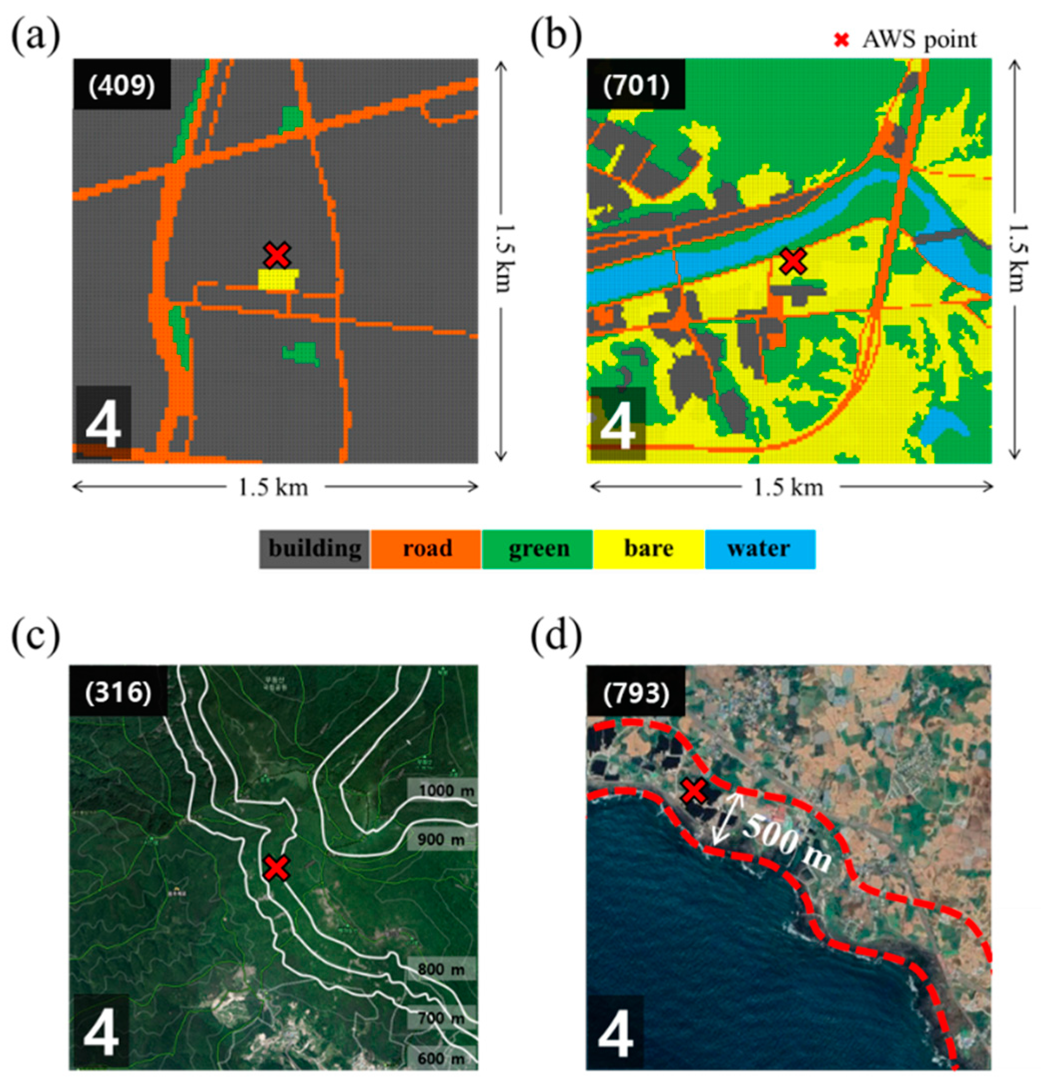
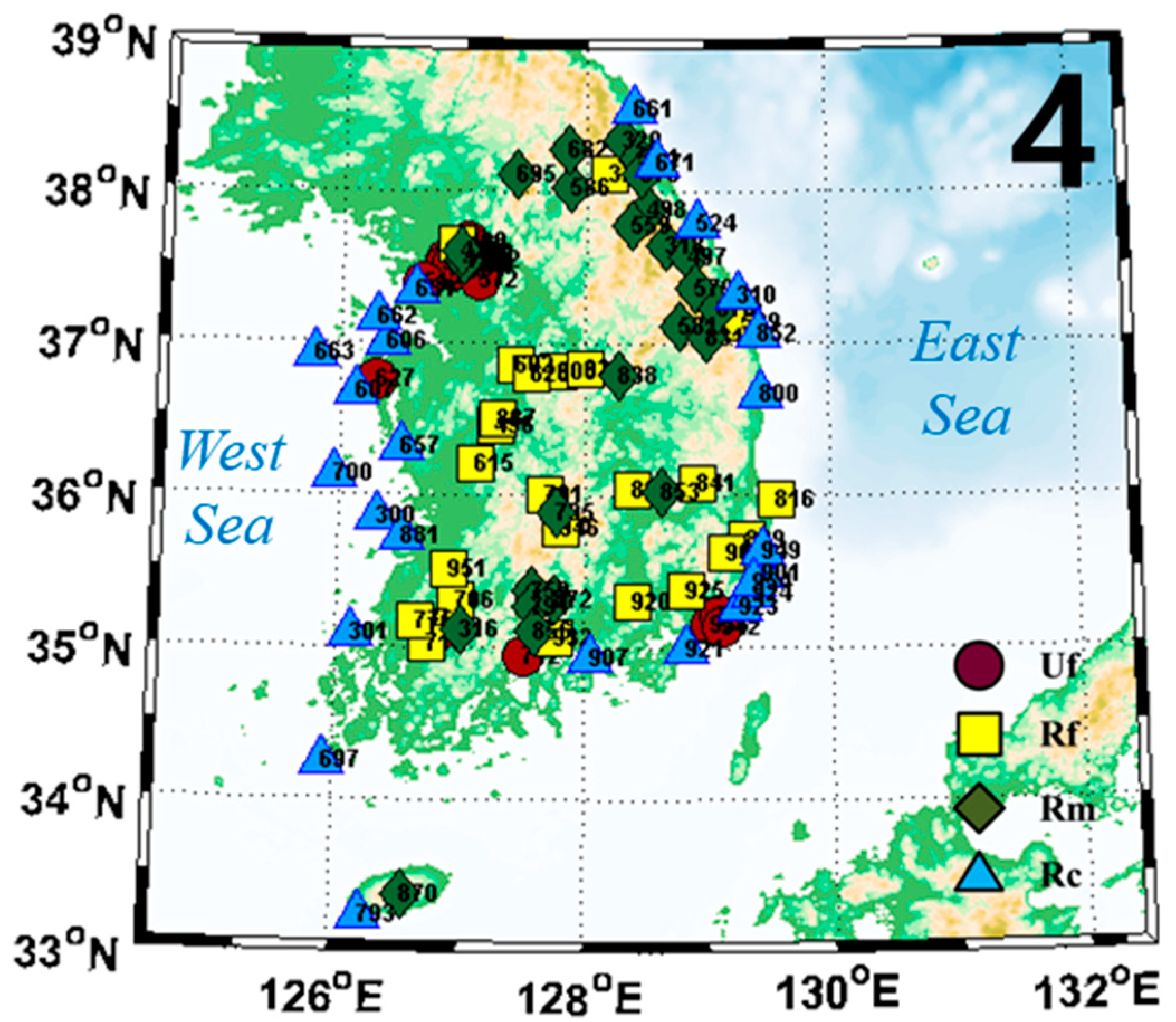
2.1. AWS Classification

First, we followed previously described classification methods [25,26,27] to characterize the region (1.5 × 1.5 km2, to match the horizontal LDAPS grid) surrounding each of 100 AWSs using land cover and topography data obtained from 1:25,000 land cover maps provided by the environmental geographic information service (EGIS) of the Ministry of Environment, Korea (Figure 1). For example, if the region surrounding an AWS had a ratio of urban (U) to rural (R) land cover of >50%, then that AWS was classified as U; otherwise, it was classified as rural R [25]. Topography was classified based on digital maps created by the National Geographic Information Institute of Korea in 2015. An AWS with altitude of >200 m in the surrounding area was classified as mountainous (m) [26]. An AWS located within horizontal distance of 500 m of a coastline was classified as coastal (c) [27]. Any AWS not classified as m or c was considered on flat terrain (f). The combination of both classification schemes yielded six categories: Um, Uc, Uf, Rm, Rc, and Rf. However, preliminary classification showed that AWSs in the Um and Uc categories were very rare in Korea. Therefore, in this study, we selected 25 AWSs (Figure 2) for each of the four remaining categories (Uf, Rm, Rc, and Rf) to identify the characteristics of LDAPS-predicted wind speeds and temperatures. Dynamical and biophysical effects of land covers are not considered in the analysis.

2.2. LDAPS Data

We used the surface wind speeds and temperatures predicted by LDAPS from January 1 to December 31, 2015. LDAPS employs a self-analysis and prediction circulation system based on a three-dimensional variational data assimilation technique [19]. LDAPS performs 36 h predictions at 00, 06, 12, and 18 UTC for the prediction and data assimilation purposes and 3 h predictions at 03, 09, 15, and 21 UTC for the data assimilation only. LDPAS assimilates various surface and upper air observation datasets after the quality control process of LDAPS automatically selects datasets that will be included and excluded in the assimilation process. The AWS observations selected in the assimilation process may hinder the data independence in the analysis. However, most of the AWS observations are known to be excluded in the assimilation process. To consider LDAPS data expected to have minimal errors, we used the initial data of LDAPS at each operation time (that is, every 3 h from 00 UTC to 21UTC) and 1 and 2 h prediction data at the rest times (that is, 01, 02, 04, 05, …, 22, and 23 UTC). Table 1 summarizes the LDAPS configuration; further details are provided elsewhere [28,29]. The horizontal and vertical grid systems are based on the Arakawa C-grid and Charney-Phillips staggered grid, respectively [30]. LDAPS employs New Dynamics [31] as a dynamics core, JULES (the Joint UK Land Environment Simulator) as a land surface process, mixed-phase scheme [32] for microphysics, and Edward-Slingo general 2-stream scheme [33] for the radiative process.
For comparison to the observations, we used LDAPS-predicted wind speeds and temperatures extracted to the same observation heights above the ground surface, even taking the building heights into account in cases of the AWSs installed above the building roofs. LDAPS does not have any grid cell including two or more AWSs. Meteorological variables predicted at a grid point by LDAPS represent those averaged over the 1.5 × 1.5 km2 area around the grid point. On the other hand, the observations at an AWS give meteorological information at one point, not reflecting the effects of the observation environment in the area as wide as the grid cell of LDAPS. Despite the difference in data representativeness, we conducted a point-based comparison of LDAPS predictions to the AWS observations due to the evaluation data availability. Hence, our analysis has the limitation of the nonequivalent representativeness of data used in the comparison.

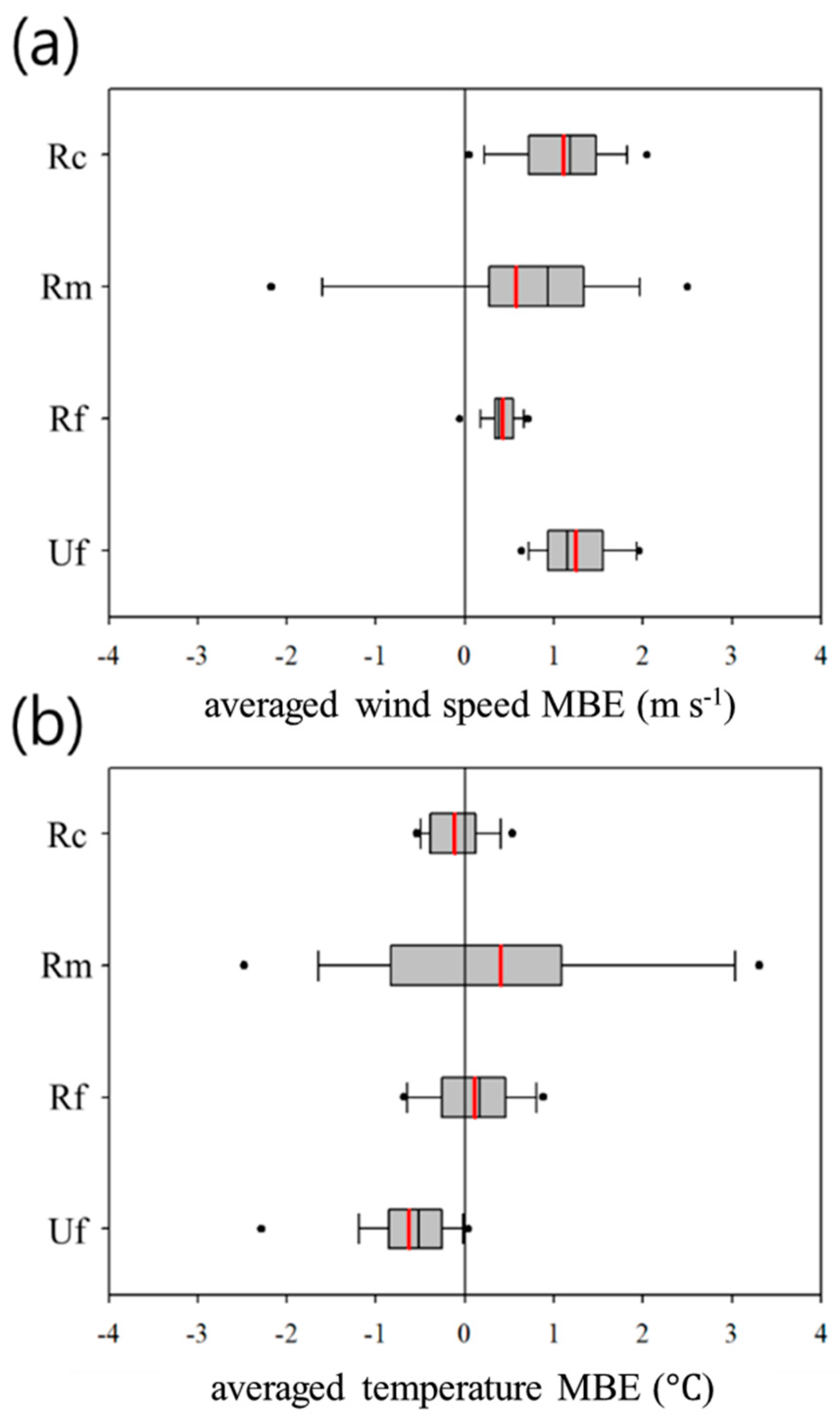
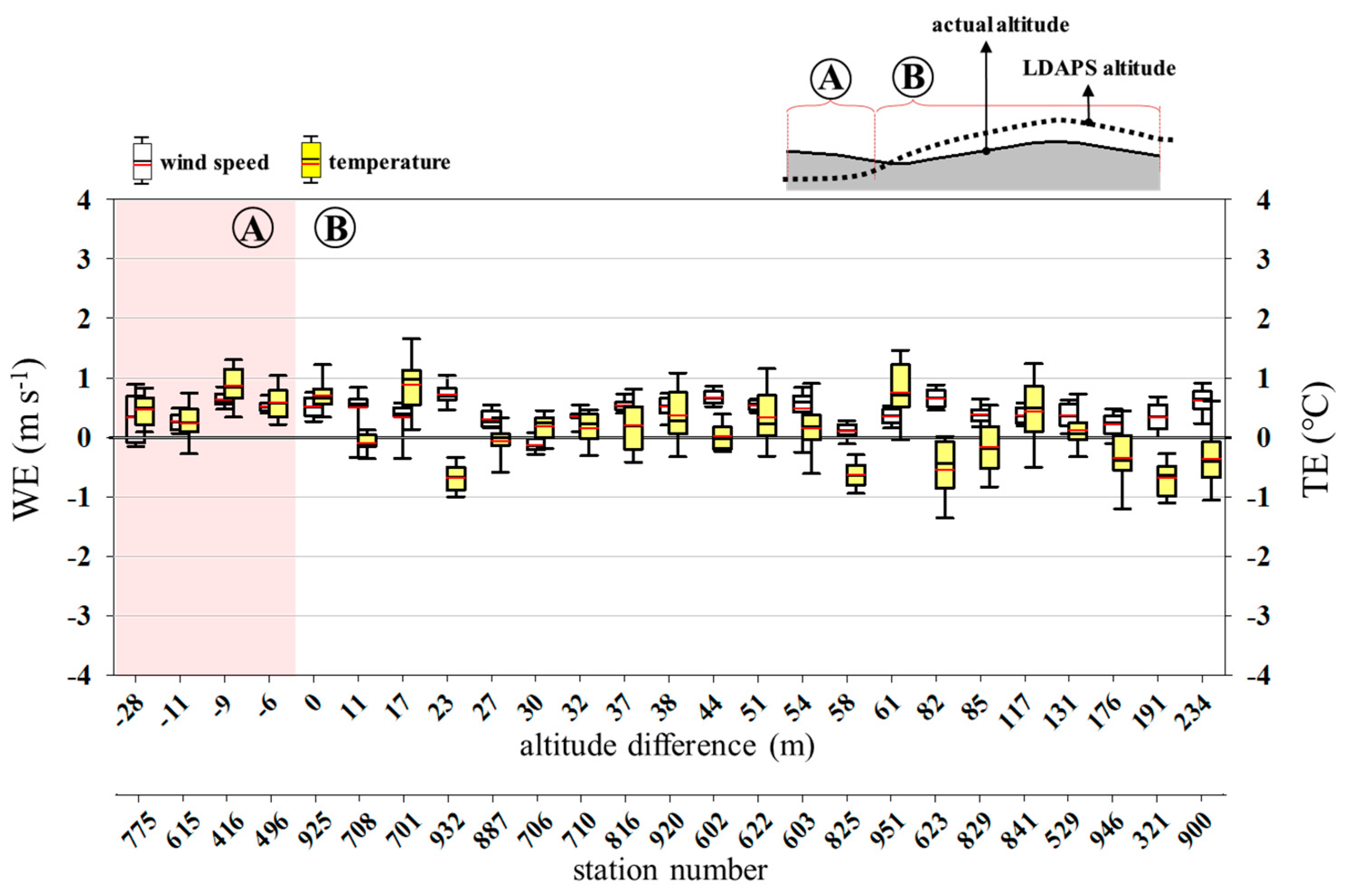
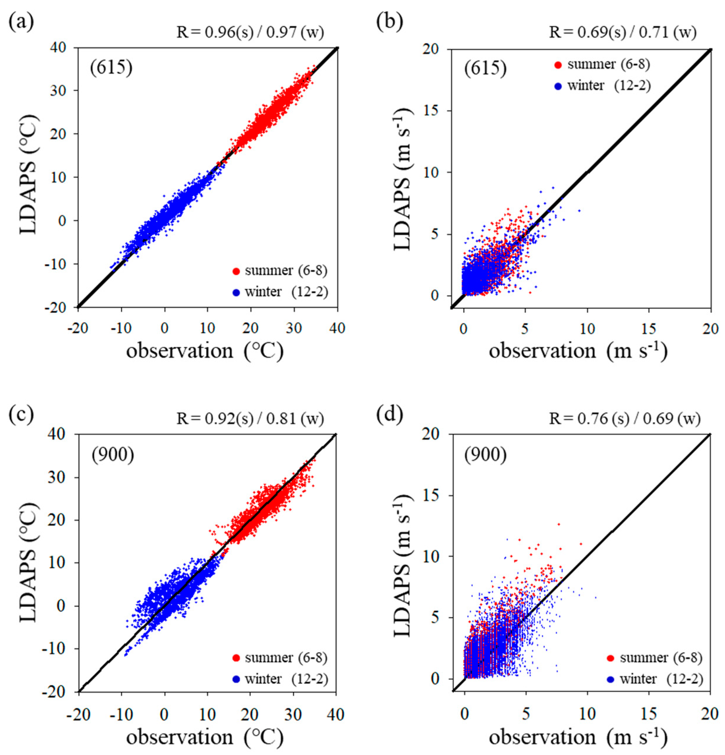
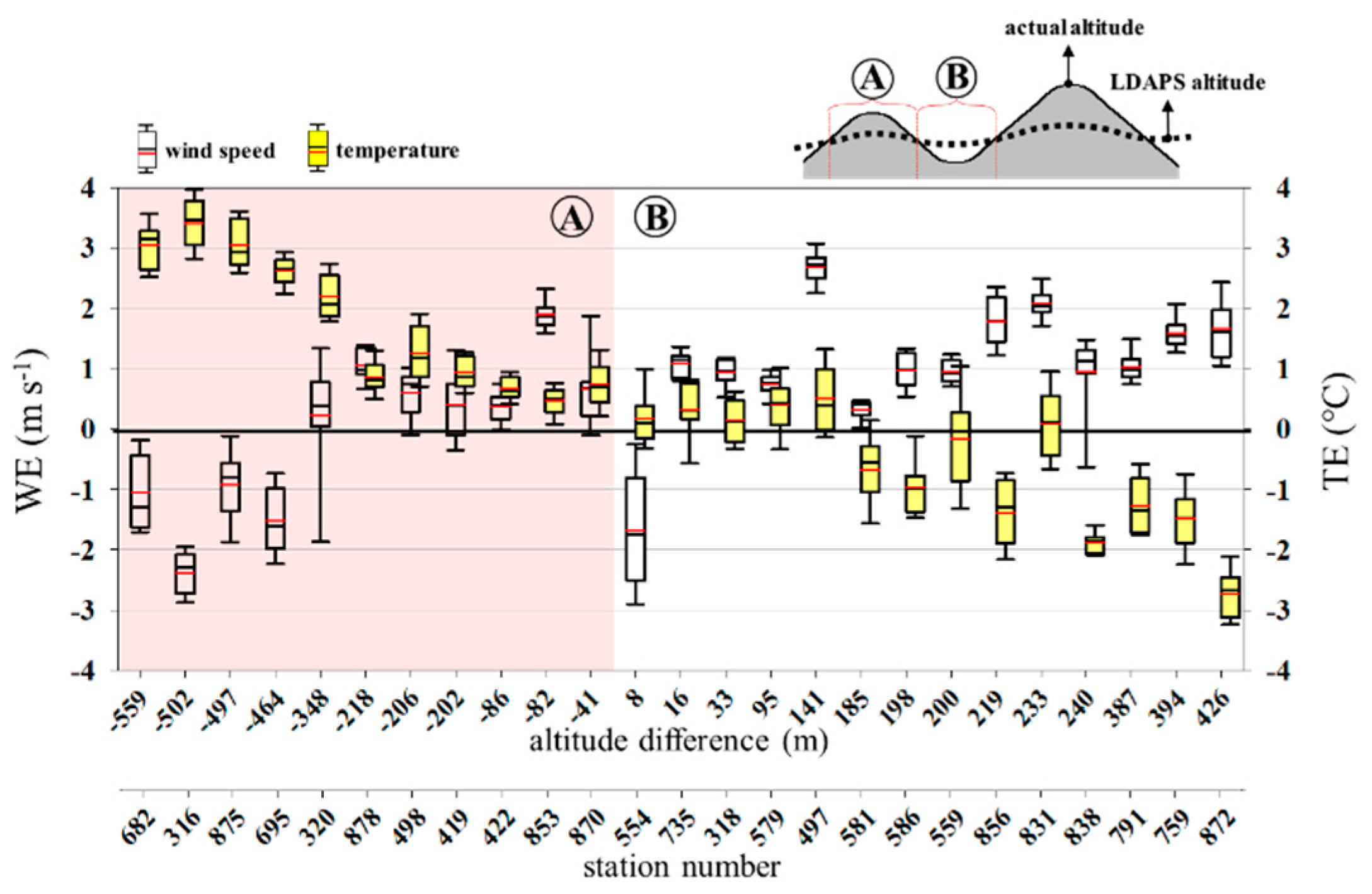
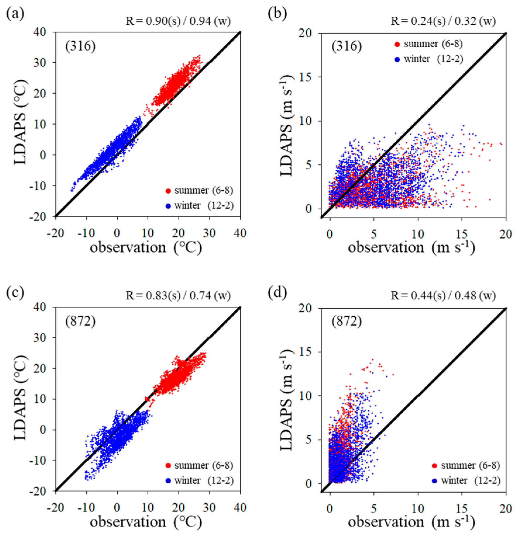
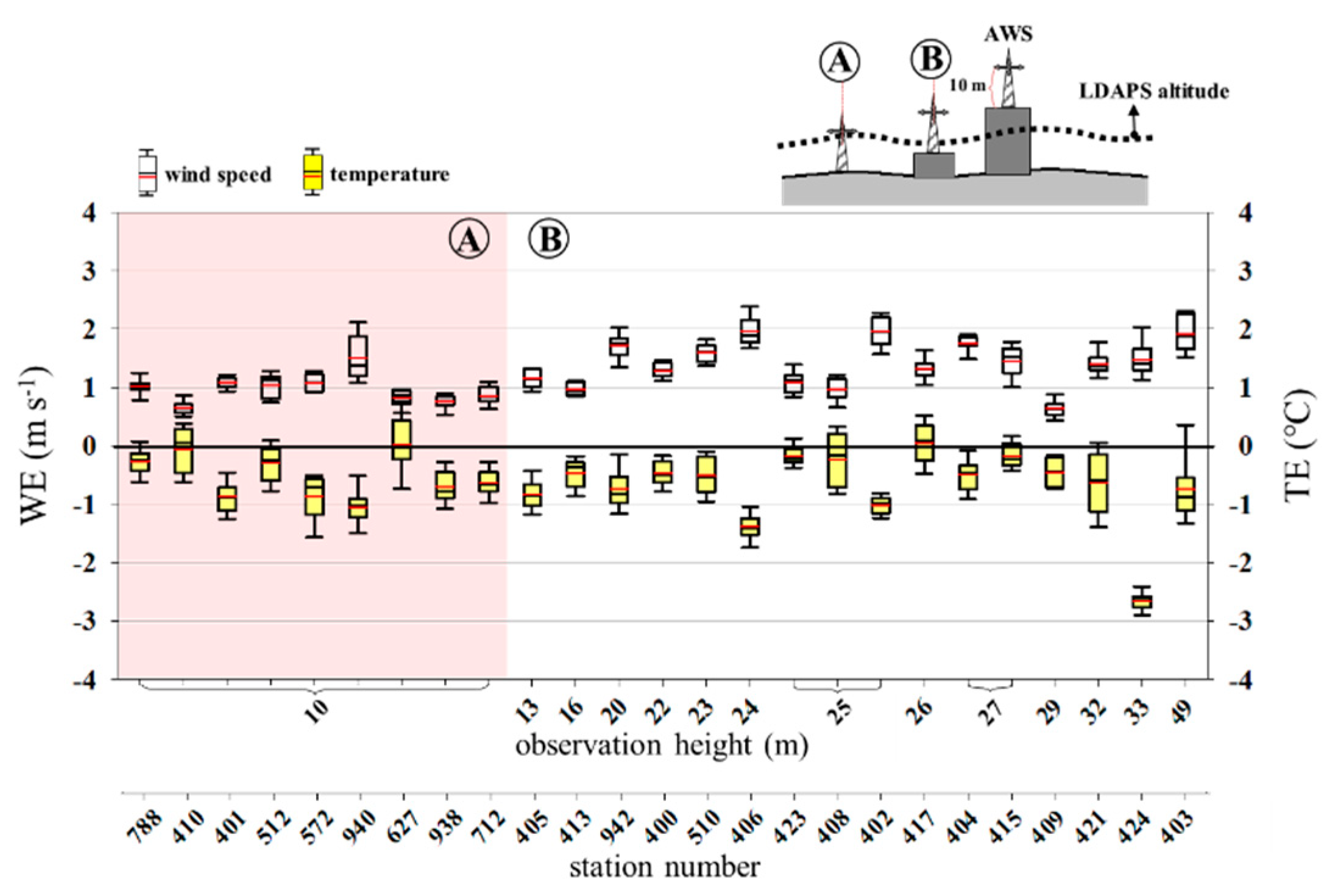
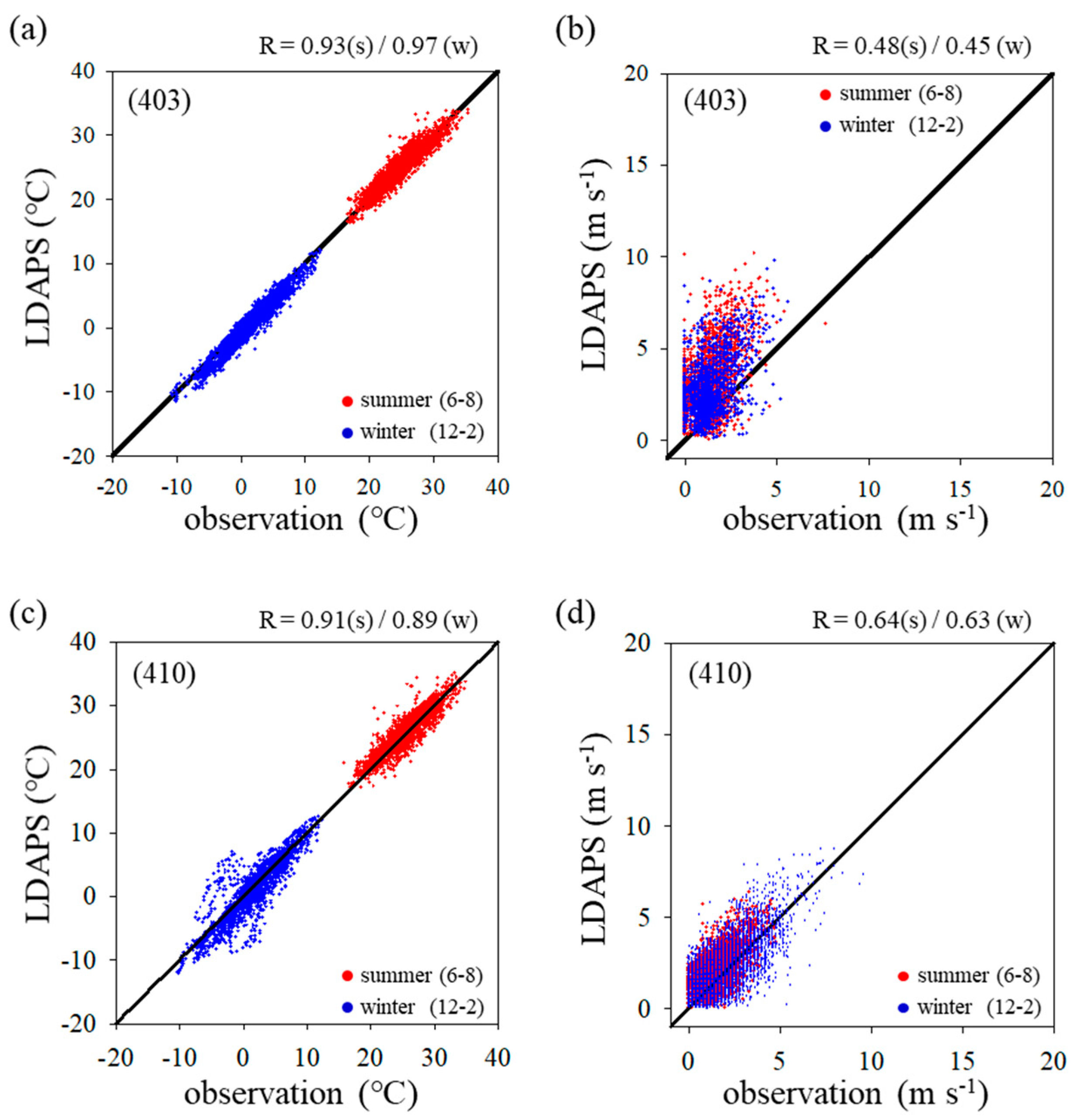
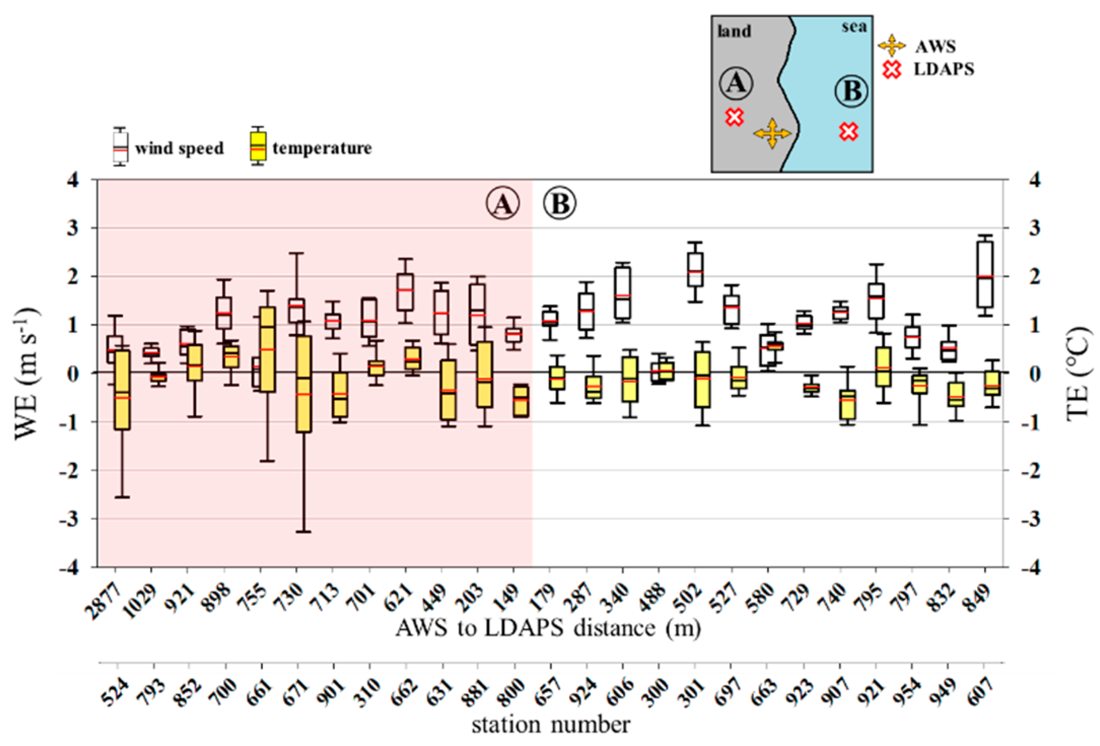
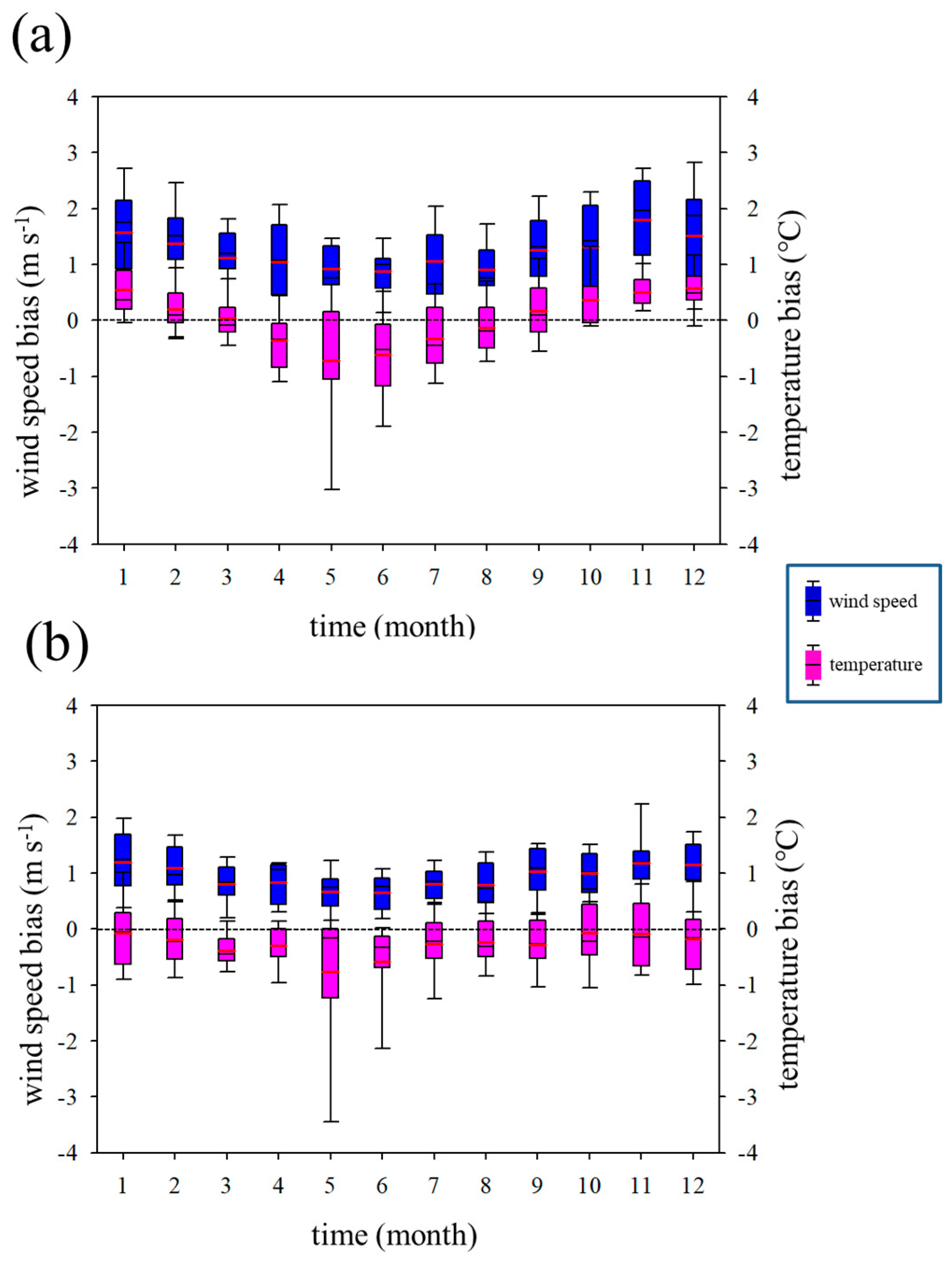
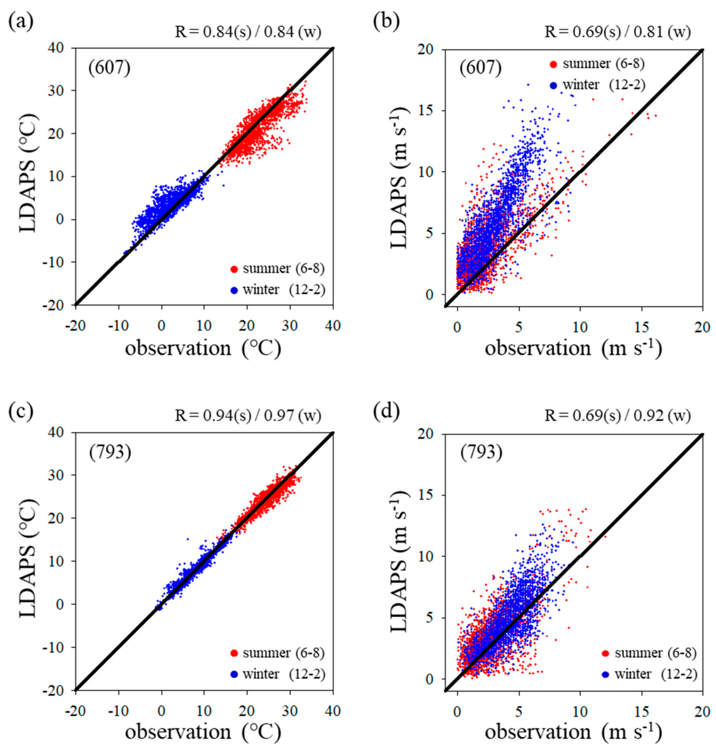
3. Results and Discussion

We calculated the mean bias error (MBE) of LDAPS prediction results for the 25 AWSs in each category during the study period and compared their averages. For details of the AWSs considered in this study, see Table A1 in Appendix A. Figure 3 shows boxplots of the MBE of wind speed (WE) and temperature (TE) for the four categories. In all categories, LDAPS generally overestimated the measured wind speed. Average WE was highest in Uf (1.26 m s−1) and lowest in Rf (0.42 m s−1). Rm showed the widest variation in WE (−2.38 to 2.68 m s−1), but a lower average (0.57 m s−1) than Rc, which had an average WE of 1.06 m s−1 (standard deviation (SD) = 0.52 m s−1). LDAPS overestimated surface wind speeds at all AWSs (Figure 3a).
At Uf AWSs, TE showed the opposite pattern to WE (Figure 3b). LDAPS underestimated temperatures at most Uf AWSs, with an average TE of −0.63 °C, which was the most significant difference among the four categories. At Rf AWSs, there was no distinct pattern in TE; LDAPS overestimated the surface temperature at some AWSs and underestimated it at others. However, as observed for average WE values, the average TE (0.12 °C) and its SD (0.46 °C) were lower than those of the other categories. At Rm AWSs, the variation in TE was highest (1.56 °C), but its average was not very high (0.41 °C). The lowest average TE (−0.12 °C) and SD (0.31 °C) were observed at Rc AWSs.
Next, we analyzed the LDAPS prediction characteristics in detail, using the relationships between MBE and the land cover and topography surrounding the AWSs in each category. Figure 4 shows WE and TE for Uf AWSs. Numerical weather prediction models are well known to overestimate the roughness lengths and surface wind speeds [34,35,36] in urban areas because most of them did not sufficiently reflect the effects of roughness such as buildings. LDAPS overestimated wind speeds measured at a height of 10 m and underestimated temperatures measured at a height of 1.5 m at most Uf AWSs (Figure 4). Notably, the TE averages at AWSs 627 and 417 were slightly greater than zero. LDAPS employs the Joint UK Land Environmental Simulator (JULES) as a land surface model; using the mosaic method within a single grid, JULES classifies land cover into nine types and applies an urban parametrization weighted by the average of each type [37]. However, the limited resolution of LDAPS prevents it from accurately reflecting flow changes caused by buildings and differential heating among land use types in urban areas [38]. As most Uf AWSs were located on building roofs, LDAPS overestimated wind speeds and underestimated temperatures (Figure 4). Correlations between AWS measurements and LDAPS predictions were slightly better in summer (June, July, and August) than winter months (December, January, and February) (Figure 5).
LDAPS overestimated wind speeds at Rf AWSs except for AWS 706, and underestimated temperatures at nine AWSs (Figure 6). The WE (<1 m s−1) and TE (<1 °C) of Rf AWSs were consistently lower than those of Uf AWSs, with averages of 0.43 m s−1 and 0.12 °C, respectively (Figure 3). This result was expected because there were few buildings to create drag and act as heat sources; thus, LDAPS performed well in predicting wind speed and temperature at Rf AWSs (Figure 3). Note that LDAPS slightly overestimated wind speed except at AWS 706, and negative TE was observed only when LDAPS altitude was higher than the actual altitude, at AWSs 321, 623, 708, 825, 829, 887, 900, 932, and 946. At AWSs 321, 900, and 946, LDAPS altitude was much higher (>170 m) than the actual altitude, and WE and TE showed similar characteristics to those of the Rm AWSs described below, i.e., wind speed overestimation and temperature underestimation. The ratio of urban areas was close to 50% at AWSs 708 (38%), 829 (46%), and 932 (48%), resulting in negative TE. AWS-measured and LDAPS-predicted temperatures were very strongly correlated, with R values of 0.96 in summer and 0.97 in winter, at AWS 615, which was located in a flat rural area, and less strongly correlated, with R values of 0.92 in summer and 0.81 in winter, at AWS 900, which was located in a basin area with a range of altitudes (Figure 7). The measured and predicted wind speeds were weakly correlated at both AWS 615 (R = 0.69 in summer and 0.71 in winter) and AWS 900 (R = 0.76 in summer and 0.69 in winter), indicating that LDAPS performed better in predicting wind speeds at Rf AWSs than at Uf AWSs (Figure 5b,d and Figure 7b,d). Further investigation showed that the LDAPS altitude was higher than the actual altitude at AWS 900, resulting in wind speed overestimation and more frequent temperature underestimation.
The variation in WE and TE was greatest at Rm AWSs among the four categories (Figure 3). At Rm AWSs, WE generally had the opposite sign to TE. WE (TE) increased (decreased) as the difference between the LDAPS and actual altitude increased (Figure 8) because LDAPS inevitably smoothed the steep terrain to avoid model blowup. Thus, for AWSs on mountain peaks or ridges, the LDAPS altitude was generally lower than the actual altitude. LDAPS resultantly underestimated (overestimated) wind speed (temperature), which is considered as a fundamental problem of numerical models for mountainous terrain [39]. By contrast, for AWSs in valleys or basins, the LDAPS altitude was generally higher than actual altitude, leading to overestimation (underestimation) of wind speed (temperature). Thus, MBE distributions distinctly reflected systematic LDAPS errors caused by smoothing (Figure 8). TE had a monotonic relationship with the altitude difference, whereas WE had a more complicated relationship, due to local circulation patterns in mountains and valleys around AWSs that were not resolved by LDAPS [40,41]. Further studies should perform more detailed analyses of these relationships. Figure 9 shows scatterplots of wind speed and temperature at AWSs 316 and AWS 872. Temperature (wind speed) was distinctly overestimated (underestimated) at AWS 316, where the LDAPS altitude was lower than the AWS altitude, and underestimated (overestimated) at AWS 872, where the LDAPS altitude was higher than the AWS altitude. At AWS 316, predicted and observed temperatures were strongly correlated (R = 0.90 in summer and 0.94 in winter). However, predicted and observed wind speeds were very poorly correlated (≤0.32), showing apparent underestimation. The correlation between measured and predicted temperatures (wind speeds) at AWS 872 was weaker (stronger) than that at AWS 316, showing apparent underestimation (overestimation).
The average WE of Rc AWSs was comparable to that of Uf AWSs (Figure 3). At Rc AWSs, wind speed was overestimated, regardless of whether the LDAPS grid points were on sea or land (Figure 10). The highest WE occurred at AWS 301, which was located on the sea. The average WE for AWSs near the West Sea (AWSs 300, 301, 606, 607, 631, 657, 662, 663, 697, 700, and 881) and East Sea (AWSs 310, 524, 661, 671, 800, 852, 901, 923, 924, 949, and 954) were 1.28 and 0.83 m s–1, respectively. The coastline of the Korean Peninsula is more complicated near the West Sea than the East Sea. However, LDAPS simplified the coastline to a greater extent near the West Sea than the East Sea, resulting in greater overestimation of wind speed. LDAPS tended to underestimate temperature when the LDAPS grid points of the AWS were on the sea (right panel, Figure 10). TE and its variation were lower for AWSs on the sea than for those on land (left panel, Figure 10). We further analyzed monthly averages of WE and TE. The average monthly WE and SD tended to increase in winter and decrease in summer (Figure 11). In spring and summer, LDAPS underestimated temperatures at AWSs with LDAPS grid points on the sea (Figure 11a), where lower sea temperatures induced negative TE. Higher sea temperatures resulted in positive TE in the fall and winter. However, at AWSs with LDAPS grid points on land, LDAPS generally slightly underestimated temperature, regardless of the season (Figure 11b). The AWS-measured and LDAPS-predicted wind speeds and temperatures were more strongly correlated in winter than in summer (Figure 12). Wind speed correlations at Rc AWSs were highest among the four categories.
Next, we analyzed WE and TE at 25 AWSs within in each category. Based on this analysis, we summarized the characteristics of wind speeds and temperatures predicted by LDAPS for Uf, Rf, Rm, and Rc (Table 2). At Uf AWSs, the average WE was >0.63 m s−1, and the average TE was <0.04 °C. At Rf AWSs, the average WE ranged from −0.12 to 0.72 m s−1. The average TE was dependent on the altitude difference between LDAPS and the actual terrain, with values > 0.24 °C when LDAPS altitude was lower than actual altitude and values ranging from −0.68 °C to 0.89 °C when LDAPS altitude was higher than actual altitude. At Rm AWSs, WE and TE was also dependent on the difference between LDAPS altitude and actual altitude, because LDAPS smoothed steep terrains in mountains and valleys. Jiménez and Dudhia [42] reported that the smoothed terrain in a numerical weather prediction model causes errors in predicting wind speeds by failing to capture momentum fluxes from unresolved topography. When the altitude difference was less (more) than 400 m, the average WE was lower (higher) than −0.92 (0.32) m s−1 except at one AWS (554). The average TE was higher (lower) than 0.14(−0.15) °C at altitude differences of less (more) than 150 m except at one AWS (831). At Rc AWSs, average WE and TE values were influenced by whether the LDAPS grid was on sea or land. At AWSs corresponding to LDAPS grid points on the sea, the average WE was >0.04 m s−1, and the average TE varied seasonally, with values >0.19 °C in fall and winter and <0.02 °C in spring and summer. At AWSs corresponding to LDAPS grid points on land, the average WE was >0.14 m s−1, and the average TE ranged from −0.56 to 0.46 °C, similar to those of Rf AWSs.

4. Summary and Conclusions

We analyzed the characteristics of surface wind speeds and temperatures predicted by LDAPS for 100 AWSs classified into four categories based on surrounding land covers and topography.
At Uf AWSs, LDAPS did not sufficiently reflect the influence of building drag and surface heating due to limited grid resolution and the applied coordinate system. At Uf AWSs, it generally overestimated wind speed (average WE = 1.26 m s−1) and underestimated temperature (average TE = −0.63 °C). At Rf AWSs, it performed best in predicting wind speed and temperature (average WE = 0.42 m s−1, average TE = 0.12 °C), because there were few buildings to provide friction and heat around the AWSs. The average WE and TE of LDAPS predictions were very small in mountainous terrain (Rm) despite their extensive variation. At Rm AWSs, WE and TE were strongly correlated with the difference between LDAPS altitude and actual altitude. LDAPS underestimated wind speed and overestimated temperature when the LDAPS terrain was lower than the actual terrain, and vice versa. In coastal terrain (Rc), it overestimated wind speed, regardless of whether the LDAPS grid points corresponded to land or sea; WE was generally slightly higher for grid points on land than for those on the sea. TE and its variation were smaller for grid points on the sea than for those on land.
Our results demonstrate that LDAPS performance in predicting wind speed and temperature at AWSs depends on the surrounding land cover (urban or rural areas) and topography (mountainous, coastal, or flat terrain). We expect that the results would help researchers (including LDAPS improvers and users) to understand the characteristics of LDAPS-predicted surface wind speed and temperature around any concerning region. Additionally, our findings will contribute to future applications of LDAPS for forecasting local weather in Korea.

Author Contributions

Conceptualization, D.-J.K. and J.-J.K.; methodology, D.-J.K. and J.-J.K.; formal analysis, D.-J.K., G.K., D.-Y.K. and J.-J.K.; writing—original draft preparation, D.-J.K., G.K., and J.-J.K.; writing—review and editing, J.-.J.K.; visualization, D.-J.K., G.K., and D.-Y.K.; funding acquisition, J.-J.K. All authors have read and agreed to the published version of the manuscript.

Funding

This work was funded by the Korea Meteorological Administration Research and Development Program under Grant ‘KMI2018-06610’ and ‘KMI2017-02410’.

Acknowledgments

The authors would like to thank the anonymous reviewers for their valuable comments and suggestions.

Conflicts of Interest

The authors declare no conflict of interest.

Appendix A. Heights of the AWSs Considered in this Study and Statistical Details

Table A1. Height of the AWSs considered in this study and statistical details.
Cate GoryStation NumberStation Height above the Mean Sea Level (m)MBE (Wind Speeds/Temperature)RMSE (Wind Speeds/Temperature)R (Wind Speeds/Temperature)Cate GoryStation NumberStation Height above the Mean Sea Level (m)MBE (Wind Speeds/Temperature)RMSE (Wind Speeds/Temperature)R (Wind Speeds/Temperature)
Uf400601.29/−0.471.82/1.260.53/0.95Rm316912−2.38/3.404.16/3.800.28/0.92
401421.08/−0.881.52/1.490.67/0.943187700.93/0.141.51/2.290.76/0.85
402571.96/−1.022.47/1.500.51/0.9632012630.23/2.192.36/2.460.53/0.93
403541.92/−0.742.50/1.410.46/0.954192660.40/0.931.79/1.850.45/0.92
404791.75/−0.492.29/1.100.52/0.954223330.37/0.671.41/1.220.49/0.96
405101.15/−0.841.61/1.440.58/0.944976582.68/0.503.36/2.800.56/0.79
406561.96/−1.392.88/2.120.46/0.9349810150.60/1.251.97/1.780.36/0.93
408490.96/−0.241.71/1.390.47/0.94554770−1.69/0.172.31/1.760.77/0.87
409400.63/−0.450.87/1.290.54/0.965595750.95/−0.161.73/2.640.72/0.87
410340.65/−0.051.10/1.480.63/0.905796090.74/0.391.36/2.280.64/0.88
413280.97/−0.471.37/1.200.51/0.965814200.32/−0.681.27/2.290.56/0.92
415331.46/−0.171.78/1.280.44/0.945862260.97/−0.981.65/2.340.62/0.92
417421.32/0.041.78/1.170.46/0.956821062−1.06/3.051.69/3.800.10/0.85
421341.40/−0.631.77/1.450.45/0.956951050−1.53/2.632.18/3.000.22/0.93
423531.08/−0.181.54/1.180.42/0.957356581.08/0.331.77/2.480.64/0.85
424561.47/−2.672.00/2.820.56/0.977594811.58/−1.492.94/3.260.40/0.73
510241.59/−0.522.11/1.330.41/0.947914131.02/−1.272.05/2.700.60/0.81
51291.03/−0.301.63/1.450.50/0.918316622.07/0.092.73/2.740.61/0.77
572291.07/−0.871.50/1.790.62/0.958384520.95/−1.891.98/2.620.64/0.92
627410.82/0.031.48/1.410.69/0.928535701.89/0.463.00/1.230.46/0.95
71290.86/−0.631.54/1.240.75/0.958565141.78/−1.332.87/2.260.62/0.87
788631.02/−0.271.68/1.370.53/0.9487014880.67/−1.392.47/2.170.62/0.84
9381090.75/−0.701.70/1.550.59/0.898728651.66/−2.733.28/3.550.46/0.79
940721.50/−1.052.46/1.820.49/0.918751596−0.92/3.043.31/3.420.47/0.90
942151.72/−0.742.24/1.300.52/0.928788141.06/0.861.87/1.540.47/0.93
Rf3212540.34/−0.681.10/2.120.71/0.92Rc300480.04/0.051.79/1.100.74/0.85
416660.64/0.871.02/2.100.69/0.9430142.09/−0.101.83/1.950.80/0.83
496300.52/0.581.20/1.750.64/0.94310141.10/0.141.58/2.390.58/0.82
529410.37/0.121.21/2.160.57/0.8552430.48/−0.511.78/2.490.49/0.83
602930.67/0.011.29/1.690.67/0.93606241.60/−0.172.11/1.490.69/0.87
6031200.48/0.161.29/1.920.72/0.9460772.00/−0.252.32/1.550.75/0.84
615120.26/0.241.01/1.300.70/0.9763191.24/−0.351.87/1.530.72/0.85
622930.54/0.331.32/2.240.75/0.92657321.07/−0.121.99/1.430.57/0.84
623750.65/−0.541.43/1.730.71/0.9566150.14/0.491.57/3.050.48/0.71
7012050.34/0.891.08/2.240.55/0.92662141.70/0.292.55/1.170.69/0.85
70649−0.12/0.181.10/1.510.69/0.94663600.51/0.552.77/1.030.77/0.91
708300.49/−0.101.26/1.300.77/0.9467131.39/−0.431.84/2.600.52/0.70
71090.36/0.161.25/1.560.79/0.9369741.35/−0.083.04/1.040.72/0.87
775510.33/0.471.08/1.330.82/0.96700521.24/0.342.68/1.060.65/0.92
816420.54/0.191.32/1.550.73/0.8979330.43/−0.061.81/1.060.81/0.95
825300.11/−0.630.95/1.830.67/0.9380090.81/−0.561.76/2.020.57/0.80
829710.38/−0.161.13/1.700.77/0.94852410.61/0.141.67/1.710.75/0.91
8411370.37/0.440.94/2.560.70/0.89881131.20/−0.131.70/1.530.54/0.82
887330.31/−0.061.04/1.540.73/0.94901681.08/−0.421.99/1.450.65/0.90
9001220.62/−0.361.42/2.400.72/0.87907231.27/−0.552.17/1.310.59/0.89
92080.52/0.371.28/1.730.73/0.94921741.54/0.012.98/1.440.62/0.88
925120.51/0.711.32/1.500.69/0.94923661.02/−0.291.87/1.120.64/0.91
93280.72/−0.681.24/1.300.53/0.95924241.28/−0.271.94/1.130.60/0.90
9463240.22/−0.351.00/2.340.69/0.8894940.52/−0.491.45/1.870.62/0.85
9511030.35/0.761.33/1.880.70/0.92954630.75/−0.261.65/1.530.61/0.92

References

  1. Kinney, P.L. Climate change, air quality, and human health. Am. J. Prev. Med. 2008, 35, 459–467. [Google Scholar] [CrossRef] [PubMed]
  2. Neumayer, E.; Plumper, T.; Barthel, F. The political economy of natural disaster damage. Glob. Environ. Chang. 2014, 24, 8–19. [Google Scholar] [CrossRef] [Green Version]
  3. Lesk, C.; Rowhani, P.; Ramankutty, N. Influence of extreme weather disasters on global crop production. Nature 2016, 529, 84. [Google Scholar] [CrossRef] [PubMed]
  4. Ayugi, B.; Tan, G.; Rouyun, N.; Zeyao, D.; Ojara, M.; Mumo, L.; Ongoma, V. Evaluation of meteorological drought and flood scenarios over Kenya, East Africa. Atmosphere (Basel) 2020, 11, 307. [Google Scholar] [CrossRef] [Green Version]
  5. Koetse, M.J.; Rietveld, P. The impact of climate change and weather on transport: An overview of empirical findings. Transp. Res. Part D Transp. Environ. 2009, 14, 205–221. [Google Scholar] [CrossRef]
  6. Rutty, M.; Andrey, J. Weather forecast use for winter recreation. Weather Clim. Soc. 2014, 6, 293–306. [Google Scholar] [CrossRef]
  7. Ziolkowska, J.R. Economic value of environmental and weather information for agricultural decisions-a case study for Oklahoma Mesonet. Agric. Ecosyst. Environ. 2018, 265, 503–512. [Google Scholar] [CrossRef]
  8. Song, B.H. A case study of the meteorological industry for the media in the USA for promotion of private sector meteorological industry in the Republic of Korea: Based on the weather channel case. Atmosphere 2014, 24, 253–263, (In Korean with English Abstract). [Google Scholar] [CrossRef] [Green Version]
  9. Kim, H.J.; Kim, J.I.; Son, H.C. A study on the economic effects of the meteorological industry. J. Environ. Policy Adm. 2019, 27, 163–184. [Google Scholar]
  10. Jeong, J.; Lee, S.-J. A statistical parameter correction technique for WRF medium-range prediction of near-surface temperature and wind speed using generalized linear model. Atmosphere (Basel) 2018, 9, 291. [Google Scholar] [CrossRef] [Green Version]
  11. Lee, J.; Shin, H.H.; Hong, S.Y.; Jiménez, P.A.; Dudhia, J.; Hong, J. Impacts of subgrid-scale orography parameterization on simulated surface layer wind and monsoonal precipitation in the high-resolution WRF model. J. Geophys. Res. Atmos. 2015, 120, 644–653. [Google Scholar] [CrossRef]
  12. Kwun, J.H.; Kim, Y.K.; Seo, J.W.; Jeong, J.H.; You, S.H. Sensitivity of MM5 and WRF mesoscale model predictions of surface winds in a typhoon to planetary boundary layer parameterizations. Nat. Hazards 2009, 51, 63–77. [Google Scholar] [CrossRef]
  13. Shin, Y.; Yi, C. Statistical downscaling of urban-scale air temperatures using an analog model output statistics technique. Atmosphere (Basel) 2019, 10, 427. [Google Scholar] [CrossRef] [Green Version]
  14. Kim, D.J.; Lee, D.I.; Kim, J.-J.; Park, M.S.; Lee, S.H. Development of a building-scale meteorological prediction system including a realistic surface heating. Atmosphere (Basel) 2020, 11, 67. [Google Scholar] [CrossRef] [Green Version]
  15. Lee, D.B.; Chun, H.Y. Development of the Korean Peninsula-Korean aviation turbulence guidance (KP-KTG) system using the local data assimilation and prediction system (LDAPS) of the Korea Meteorological Administration (KMA). Atmosphere 2015, 25, 367–374, (In Korean with English Abstract). [Google Scholar] [CrossRef] [Green Version]
  16. Kim, D.Y.; Kim, T.W.; Oh, G.J.; Huh, J.C.; Ko, K.N. A comparison of ground-based LiDAR and met mast wind measurements for wind resource assessment over various terrain conditions. J. Wind. Eng. Ind. Aerod. 2016, 158, 109–121. [Google Scholar] [CrossRef]
  17. Park, S.-U.; Lee, I.-H.; Joo, S.J.; Ju, J.-W. Emergency preparedness for the accidental release of radionuclides from the Uljin Nuclear Power Plant in Korea. J. Environ. Radioact. 2017, 180, 90–105. [Google Scholar] [CrossRef]
  18. Kang, M.S.; Lim, Y.-K.; Cho, C.B.; Kim, K.R.; Park, J.S.; Kim, B.-J. The sensitivity analyses of initial condition and data assimilation for a fog event using the mesoscale meteorological model. J. Korean Earth Sci. 2015, 36, 567–579, (In Korean with English Abstract). [Google Scholar] [CrossRef]
  19. Yi, C.; Shin, Y.; Roh, J.W. Development of an urban high-resolution air temperature forecast system for local weather information services based on statistical downscaling. Atmosphere (Basel) 2018, 9, 164. [Google Scholar] [CrossRef] [Green Version]
  20. Wie, J.; Hong, S.O.; Byon, J.Y.; Ha, J.C.; Moon, B.K. Sensitivity analysis of surface energy budget to albedo parameters in Seoul metropolitan area using the Unified Model. Atmosphere (Basel) 2020, 11, 120. [Google Scholar] [CrossRef] [Green Version]
  21. Simón-Moral, A.; Dipankar, A.; Roth, M.; Sánchez, C.; Velasco, E.; Huang, X.Y. Application of MORUSES single-layer urban canopy model in a tropical city: Results from Singapore. Q. J. R. Meteorol. Soc. 2020, 146, 576–597. [Google Scholar] [CrossRef]
  22. Harris, P.P.; Folwell, S.S.; Gallego-Elvira, B.; Rodríguez, J.; Milton, S.; Taylor, C.M. An evaluation of modeled evaporation regimes in Europe using observed dry spell land surface temperature. J. Hydrometeorol. 2017, 18, 1453–1470. [Google Scholar] [CrossRef] [Green Version]
  23. Unnikrishnan, C.K.; Gharai, B.; Mohandas, S.; Mamgain, A.; Rajagopal, E.N.; Iyengar, G.R.; Rao, P.V.N. Recent changes on land use/land cover over Indian region and its impact on the weather prediction using Unified model. Atmos. Sci. Lett. 2016, 17, 294–300. [Google Scholar]
  24. Golding, B.W.; Ballard, S.P.; Mylne, K.; Roberts, N.; Saulter, A.; Wilson, C.; Simonin, D. Forecasting capabilities for the London 2012 Olympics. Bull. Am. Meteorol. Soc. 2014, 95, 883–896. [Google Scholar] [CrossRef]
  25. Kwon, Y.-A.; Lee, H.-Y. The characteristics of air temperature distribution by land-use type—A case study of around automatic weather station in Seoul. J. Environ. Impact Asses. 2003, 12, 281–290, (In Korean with English Abstract). [Google Scholar]
  26. Sung, C.-J. A study on the analysis of terrain element and terrain classification using GIS. Geogr. J. Korea 2003, 37, 155–161, (In Korean with English Abstract). [Google Scholar]
  27. Lee, J.W.; Kim, Y.S. Coastline change analysis using RTK-GPS and aerial photo. J. Korean Soc. Surv. 2007, 25, 191–198, (In Korean with English Abstract). [Google Scholar]
  28. Prasanna, V.; Choi, H.-W.; Jung, J.; Lee, Y.G.; Kim, B.J. High-resolution wind simulation over Incheon international airport with the Unified Model’s Rose Nesting Suite from KMA operational forecasts. Asia Pac. J. Atmos. Sci. 2018, 54, 187–203. [Google Scholar] [CrossRef]
  29. Walters, D.N.; Williams, K.D.; Boutle, I.A.; Bushell, A.C.; Edwards, J.M.; Field, P.R.; Willett, M.R. The Met Office Unified Model global atmosphere 4.0 and JULES global land 4.0 configurations. Geosci. Model Dev. 2014, 7, 361–386. [Google Scholar] [CrossRef] [Green Version]
  30. Charney, J.G.; Phillips, N.A. Numerical integration of the quasi-geostrophic equations for barotropic and simple baroclinic flows. J. Atmos. Sci. 1953, 10, 71–99. [Google Scholar] [CrossRef] [Green Version]
  31. Davies, T.; Cullen, M.J.P.; Malcolm, A.J.; Mawson, M.H.; Staniforth, A.; White, A.A.; Wood, N. A new dynamical core for the Met Office’s global and regional modelling of the atmosphere. Q. J. R. Meteorol. Soc. 2005, 131, 1759–1782. [Google Scholar] [CrossRef]
  32. Lock, A.P.; Brown, A.R.; Bush, M.R.; Martin, G.M.; Smith, R.N.B. A new boundary layer mixing scheme. Part 1: Scheme description and single-column model tests. Mon. Weather Rev. 2000, 128, 3187–3199. [Google Scholar] [CrossRef]
  33. Edwards, J.M.; Slingo, A. Studies with a flexible new radiation code. 1: Choosing a configuration for a large-scale model. Q. J. R. Meteor. Soc. 1996, 122, 689–719. [Google Scholar] [CrossRef]
  34. De Rooy, W.C.; Kok, K. A combined physical–statistical approach for the downscaling of model wind speed. Weather Forecast. 2004, 19, 485–495. [Google Scholar] [CrossRef]
  35. Yu, M.; Wu, B.; Zeng, H.; Xing, Q.; Zhu, W. The impacts of vegetation and meteorological factors on aerodynamic roughness length at different time scales. Atmosphere (Basel) 2018, 9, 149. [Google Scholar] [CrossRef] [Green Version]
  36. Sun, W.; Liu, Z.; Zhang, Y.; Xu, W.; Lv, X.; Liu, Y.; Lyu, H.; Li, X.; Xiao, J.; Ma, F. Study on land-use changes and their impacts on air pollution in Chengdu. Atmosphere (Basel) 2020, 11, 42. [Google Scholar] [CrossRef] [Green Version]
  37. Best, M.J. Representing urban areas within operational numerical weather prediction models. Bound. Lay. Meteorol. 2005, 114, 91–109. [Google Scholar] [CrossRef]
  38. Salamanca, F.; Zhang, Y.; Barlage, M.; Chen, F.; Mahalov, A.; Miao, S. Evaluation of the WRF-urban modeling system coupled to Noah and Noah-MP land surface models over a semiarid urban environment. J. Geophys. Res. Atmos. 2018, 123, 2387–2408. [Google Scholar] [CrossRef]
  39. Gross, G. On the parametrization of urban land use in mesoscale models. Bound. Lay. Meteorol. 2014, 150, 319–326. [Google Scholar] [CrossRef]
  40. Revell, M.J.; Purnell, D.; Lauren, M.K. Requirements for large-eddy simulation of surface wind gusts in a mountain valley. Bound. Lay. Meteorol. 1996, 80, 333–353. [Google Scholar] [CrossRef]
  41. Fast, J.D. Forecasts of valley circulations using the terrain-following and step-mountain vertical coordinates in the Meso-Eta model. Weather Forecast. 2003, 18, 1192–1206. [Google Scholar] [CrossRef]
  42. Jiménez, P.A.; Dudhia, J. Improving the representation of resolved and unresolved topographic effects on surface wind in the WRF model. J. Appl. Meteorol. Clim. 2012, 51, 300–316. [Google Scholar] [CrossRef] [Green Version]
Figure 1. Classification of the automated weather stations (AWSs) for land-use (a,b) and topography types (c,d). Red symbols and white solid lines in (c) represent AWSs and contour lines, respectively. The deviant crease lines in (d) indicate the area within 500 m from the coastline.
Atmosphere 11 01224 g001
Figure 2. The locations of the AWSs in four categories selected in this study.
Atmosphere 11 01224 g002
Figure 3. Box Plots of the (a) WEs and (b) TEs for four categories. In each box plot, upper and lower black circles indicate the outliers, the bars above and below a box, respectively, indicate the upper and lower extremes, and upper, middle, and lower segments of a box, respectively, indicate the upper quartile, median, and lower quartile. The red line in each box plot represents the average of the mean bias error for the category.
Atmosphere 11 01224 g003
Figure 4. Box plots of the WEs and TEs at the Uf AWSs. The x-axis represents observation height of the AWSs. Left panel shaded in pink (Ⓐ) is for the AWSs installed on the ground (that is, the observation height is 10 m above ground level). Right panel shaded in blue is for the AWSs installed on building roofs (Ⓑ).
Atmosphere 11 01224 g004
Figure 5. Scatter plots of the AWS-observed and LDAPS-predicted temperatures (left panels) and wind speeds (right panels) at the (a,b) AWS 403 (installed on a building roof and (c,d) AWS 410 (installed on the ground level). Red and blue dots indicate for summer season (June, July, and August) and winter season (December, January, and February), respectively.
Atmosphere 11 01224 g005
Figure 6. Box plots of the WEs and TEs at the Rf AWSs. The x-axis represents difference between the LDAPS and actual altitudes at the AWSs. Left panel shaded in pink represents the cases that the LDAPS altitudes are lower than the actual altitudes (Ⓐ). Right panel shaded in blue indicates the opposite cases (Ⓑ).
Atmosphere 11 01224 g006
Figure 7. Scatter plots of the AWS-observed and LDAPS-predicted temperatures (left panels) and wind speeds (right panels) at the (a,b) AWS 615 (located at a flat rural area) and (c,d) AWS 900 (located at a basin area). Red and blue dots indicate for summer season (June, July, and August) and winter season (December, January, and February), respectively.
Atmosphere 11 01224 g007
Figure 8. Box plots of the WEs and TEs at the Rm AWSs. Left panel shaded in pink represents the cases that the LDAPS altitudes are higher than the actual altitudes (Ⓐ). Right panel shaded in blue indicates the opposite cases (Ⓑ).
Atmosphere 11 01224 g008
Figure 9. Scatter plots of the AWS-observed and LDAPS-predicted temperatures (left panels) and wind speeds (right panels) at the (a,b) AWS 316 (LDAPS altitude < AWS altitude) and (c,d) AWS 872 (LDAPS altitude > AWS altitude). Red and blue dots indicate for summer season (June, July, and August) and winter season (December, January, and February), respectively.
Atmosphere 11 01224 g009
Figure 10. Box plots of the WEs and TEs at the Rc AWSs. Left panel shaded in blue and right panel shaded in red represent the cases that the LDAPS grid point closest to a comparison AWS is located at the land (Ⓐ) and sea (Ⓑ), respectively.
Atmosphere 11 01224 g010
Figure 11. Monthly MBEs of wind speeds and temperatures predicted by LDAPS at the Rc AWSs. The LDAPS grid point closest to a comparison AWS is located at sea in (a) and land in (b).
Atmosphere 11 01224 g011
Figure 12. Scatter plots of the AWS-observed and LDAPS-predicted temperatures (left panels) and wind speeds (right panels) at the (a,b) AWS 607 (LDAPS grid located at sea) and (c,d) AWS 793 (LDAPS grid located at land). Red and blue dots indicate for summer season (June, July, and August) and winter season (December, January, and February), respectively.
Atmosphere 11 01224 g012
Table 1. Summary of local data assimilation and prediction system (LDAPS)’s numerical details.
ModelLDAPS (UM 1.5 km L70)
Basic modelUK Met Office Unified Model (UM) Vn 8.2
horizontal grid dimensionvariable grid (total): 744 × 928fixed grid (inner): 622 × 810
horizontal grid size (km) (inner)1.5
dynamics coreNew Dynamics
horizontal grid systemArakawa C-grid
vertical layers70 (eta level) (~40 km)
time step50 s
time integrationsemi-implicit semi-Lagrangian scheme
vertical grid systemCharney-Phillips staggered grid
boundary conditionsGlobal Data Assimilation and Prediction System (GDAPS)
data assimilation3DVAR/latent heat nudging
radiative processEdward-Slingo general 2-stream scheme
land surface processJULES (Joint UK Land Environment Simulator) land-surface scheme
microphysicsmixed-phase scheme with graupel
planetary boundary layernon-local scheme with revised diagnosis of K profile depth
gravity wave draggravity wave drag due to orography
Table 2. Summary of the LDAPS characteristics for the four categories (Uf, Rf, Rm, and Rc).
CategoryPrediction Characteristics of LDAPS Model
Wind SpeedTemperature
Uf▪ If an AWS located on the ground
  0.66   <   WE   <   1.50   m   s 1 ,   IQR ¯ = 0.27 m s−1
▪ If an AWS located on the building
  0.63   <   WE   <   1.96   m   s 1 ,   IQR ¯ = 0.28 m s−1
▪ If an AWS located on the ground
  1.05   <   TE   <   0.03   ° C ,   IQR ¯   =   0.44   ° C
▪ If an AWS located on the building
  2.67   <   TE   <   0.04   ° C ,   IQR ¯   =   0 . 43   ° C
Rf 0.12   <   WE   <   0.72   m   s - 1 ,   IQR ¯ = 0.22 m s−1▪ If (LDAPS—actual altitude) < 0 m
  0.24   <   TE   <   0.87   ° C ,   IQR ¯   =   0 . 41   ° C
▪ If (LDAPS—real-terrain altitude) > 0 m
  0.68   <   TE   <   0.89   ° C ,   IQR ¯   =   0 . 45   ° C
Rm▪ If (LDAPS—actual altitude) < −400m
  2.38   <   WE   <   0.92   m   s 1 ,   IQR ¯ = 0.85 m s−1
▪ If (LDAPS—real-terrain altitude) > −400m
  1.69   <   WE   <   2.68   m   s 1 ,   IQR ¯ = 0.47 m s−1
▪ If (LDAPS—actual altitude) < 150 m
  0.14   <   TE   <   3.40   ° C ,   IQR ¯   =   0 . 56   ° C
▪ If (LDAPS—actual altitude) > 150 m
  2.73   <   TE   <   0.09   ° C ,   IQR ¯   =   0 . 70   ° C
Rc▪ If LDAPS grid located on the land
  0.14   <   WE   <   1.70   m   s 1 ,   IQR ¯ = 0.57 m s−1
▪ If LDAPS grid located on the sea
  0.04   <   WE   <   2.09   m   s 1 ,   IQR ¯ = 0.54 m s−1
▪ If LDAPS grid located on the land
  0.56   <   TE   <   0.49   ° C ,   IQR ¯   =   0 . 88   ° C
▪ If LDAPS grid located on the sea
  0.55   <   TE   <   0.55   ° C ,   IQR ¯   =   0 . 47   ° C
Note: IQR indicate inter-quartile range.
Publisher’s Note: MDPI stays neutral with regard to jurisdictional claims in published maps and institutional affiliations.

