Advanced Rainfall Trend Analysis of 117 Years over West Coast Plain and Hill Agro-Climatic Region of India

Abstract

In this paper, the rainfall trend of the West Coast Plain and Hill Agro-Climatic Region is analyzed for 117 years (1901–2017). This region is a globally recognized biodiversity hotspot and known for one of the highest rainfall receiving regions in India. Rainfall grid dataset is used for the analysis of rainfall trends on monthly, seasonal, and decadal time scales. Modified Mann–Kendall’s test, Linear Regression, Innovative Trend Analysis, Sen’s Slope test, Weibull’s Recurrence Interval, Pearson’s Coefficient of Skewness, Consecutive Disparity Index, Kurtosis, and some other important statistical techniques are employed for trend analysis. Results indicate that the rainfall trend is significant in January, July, August, September as well as the Winter season. Among all the significant trends, January and July showed a decreasing rainfall trend. July has the highest contribution (30%) among all the obtained monotonic trend to annual rainfall and coincidentally has the highest trend magnitude. August and September months with a combined contribution of 30% to annual rainfall, show an increasing monotonic trend with high magnitude whereas Winter season shows a monotonic decreasing rainfall trend with comparatively low magnitudes. Decadal analysis along with the study of recurrence interval of excess and deficit years helps to understand the decadal rhythm of trend and the magnitude of extreme monthly and seasonal events. Skewness reveals that rainfall dataset of all the periodic results is right-skewed and the recurrence interval also supports the skewness results. Sharply decreasing rainfall in July and rising rainfall in August and September is predictive of the impact on agriculture, biodiversity and indicates the rainfall regime shift in the region.

1. Introduction

Climate change is gradual and comparatively more stable than climate variability phenomena. Nevertheless, the climate has been dynamic in the past and as per its nature, it will remain so in the future [1,2,3,4,5]. The scientific tempered community has always supported the practice to analyze the trend of a homogeneous climatic region with appropriate statistical techniques. Rainfall and temperature trend has been analyzed for different parts of the world. In light of climate change, rainfall is on high focus due to the importance of water for the survival of various ecosystems on the earth. Concerning the trend, it is always good to have the necessary statistical significance for confidence in the occurrence of the event. This becomes very challenging because of the availability of instrumental observations for a short time-span.

Many studies for different regions on the globe are completed using the station and grid dataset to analyze the trend of rainfall for a long period. Some regions on earth are very important for the environment and stability of the regional economy. The coast of Tanzania is one good example of an economic hotspot of the world and therefore an analysis of rainfall trends was completed for the region [6]. Doing the spatial analysis of rainfall for Brazil, it is reported using linear tendencies that rainfall significantly (95% significance level) increased in northern Amazon and decreased in southern Brazil [7]. Frazier and Giambelluca [8] reported the existence of a multi-decadal variability and drying trend, which is significant for the whole Hawaiian state only for the recent decade. In the European case, a highly significant decline is observed in southern Italy in the past 30 years of the analysis period 1918–1999 [9]. Weaker meridional circulation due to the absence of trough at 850 mb and weaker easterly jet at 200 mb is credited for negative rainfall trend in the Sahel of North Africa [10].

Most of the time, the climate of each region on the Earth has good teleconnection with one or the other atmospheric, oceanic or coupled phenomena. Consequently, it influences the rainfall and temperature prevailing in those regions. Studies related to teleconnection have been broadly discussed in different perspectives. In an Indian perspective, the teleconnection of tropical climate modes such as El Niño, La Niña, El Niño Modoki, La Niña Modoki, Positive Indian Ocean Dipole, Negative Indian Ocean Dipole is studied extensively [11,12,13,14,15,16] and teleconnection of West Coast Plain and Hill Agro-Climatic (hereafter WCPHAC) region has also been studied [17,18,19]. In a study over a small part of the WCPHAC region, Manjunatha et al. [18] found that the Oceanic Niño Index has an inverse relationship with summer rainfall over the Western Ghats.

The rainfall trend of a river basin within the WCPHAC region containing 28 rain gauge stations shows a significant trend for annual, monsoon, and pre-monsoon period [20]. Trend analysis is conducted using rainfall, temperature, and streamflow data of different river catchments of the Western Ghats. A significant trend is obtained with Mann–Kendall’s test and rainfall trend (1950–2015) is found significant on a seasonal basis for a southernmost river catchment in Western Ghats [21]. Prakash et al. [22] studied the trend for 32 years using the satellite imageries and found the decreasing trend in rainfall from July to August season.

Rainfall over the WCPHAC region has a lot of importance for various phenomena over Peninsular India such as river flow of the various peninsular river, water for biodiversity in the Western Ghats, moisture supply, etc. [23]. Orographic rainfall occurs on the mountainous peaks and causes rain shadow zone to the east of Western Ghats [24]. A study for the southern part of the Western Ghats for 30 years (1981–2010) has shown the declining rainfall during southwest monsoon with decreasing (increasing) moderate (high intensity) rainfall events [25]. In another study, data of 23 stations at the pan-Indian level have reported the significant trend results for stations on the west coast of India [26]. The declining trend in the rainfall at the end of the 19th century and increasing trend after 1920 has been reported [27]. No long-term trend is observed for the west coast stations in India with data used for a varying period of different stations [28]. Stations on the western coast are part of the WCPHAC region, which is the platform where southwest monsoon’s first performance is observed. The performance of southwest monsoon rainfall is assumed as the index of rainfall performance across the South Asia subcontinent. This region is one of the biodiversity hotspots in India and the eighth hottest hotspot of biodiversity in the world [29]. Western Ghats in the WCPHAC region is a natural barrier for the southwest monsoonal rainfall in the WCPHAC region and also known as one of the highest rainfall belts along with the Arakan Yoma in the summer monsoon belt [22].

Due to the similarity of the Western Ghats and Arakan Yoma, a study by Shrestha et al. [30] discusses the characteristics of precipitation in both the regions for 13 years during the summer monsoon season and found the intense rainfall in offshore regions. The dissimilarity of the rainfall distribution and trend at the regional level is observed in all of these important studies and therefore, the WCPHAC region being agro-climatic region is selected for rainfall trend analysis.

WCPHAC in particular and India in general is highly prone to land degradation, soil erosion, radiological pollution & contamination, forest loss, etc. [31,32,33,34,35,36]. Knowing the WCPHAC region as the platform for monsoon onset and a biodiversity hotspot, we attempted to understand monotonic rainfall and its characteristics at monthly, seasonal, and decadal time scale. Highly acceptable statistical techniques are used for the advanced analysis of rainfall trend of 117 years in the WCPHAC region. The occurrence of extreme events has also been identified and analyzed for all the monotonic trend results. This study elaborates on the monotonic rainfall trend for the WCPHAC region as a unit as well as a trend at each grid point of the used rainfall gridded dataset. As a result of the analysis provided in this study, it also helps to fill the gap that existed in the literature to understand the monotonic trend of rainfall at different temporal scales for WCPHAC.

Given the above, most of the studies discussed here are associated with Mann-Kendall’s test [8,9,21,28,37] and one each with Kendall rank correlation test, linear tendency, satellite image [7,20,22]. Along with trend detection of the essential climate variables, Mann-Kendall’s test can be used with any variable for the detection of a monotonic trend [38,39,40]. In the recent past, some studies have come up with results obtained using Modified Mann–Kendall’s Test (hereafter MMKT) and definitely, these results are more dependable and accurate with variance correction approaches to remove the influence of serial correlation [41,42,43]. This variance correction is required to eliminate the presence of autocorrelation [44,45].

The non-parametric test is very popular in studies related to climate change due to the high accuracy, repeatability, and flexibility [38,46,47,48]. Many non-parametric tests are available for assessment of the trend and used in hydrological studies. However, MMKT, linear regression, Innovative trend analysis (hereafter ITA), and Sen’s slope estimator were used in this study. The traditional Mann–Kendall’s test has some limitations: (1) Assumption lying in the hypothesis ($H_0$) that the dataset is independently and identically distributed and (2) Influence of autocorrelation in the data used for significance estimation. MMKT has the advantage of no influence of autocorrelation and therefore it is widely used nowadays. Whereas, the ITA test allows the trend estimation without dependence on data distribution and the influence of autocorrelation [49]. ITA test has been used widely in many studies across the globe [50,51,52]. The trend of rainfall for 152 rain gauge stations in south island in New Zealand is estimated using ITA [50]. Meena et al. [53] used ITA and Mann–Kendall’s test to analyze the trend direction of rainfall in 12 semi-arid districts of western Rajasthan in India. Caloiero et al. [54] also used ITA and Mann–Kendall’s test to estimate the trend of more than 500 rain gauge station over 50 years in Italy. Wang et al. [55] used the ITA method to find the trend of precipitation in eastern China and found the result in agreement with classical methods. The literature review reveals that no study is conducted on the long-term rainfall trend over WCPHAC using the combination of MMKT, linear regression, and ITA. ITA test is used along with MMKT and linear regression to justify the accuracy of the result obtained with their agreement with each other and to strengthen the set narrative from the results.

The remainder of this paper is organized in the following manner. Section 2 discusses the study area, data, and method used in the study. Section 3 explains the results. Section 4 presents the discussion. Finally, Section 5 draws the concluding remarks.

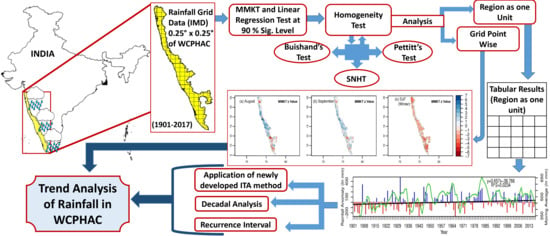
2. Materials and Methods

2.1. Study Area

Planning Commission of India delineated 15 agro-climatic regions in India on the basis of soil, rainfall and temperature, and other agro-meteorological characteristics [56,57]. The reason for the delineation was the region-specific planning to have long-term benefits in the rural sector through the use of locally available resources and by reducing the regional inequalities. WCPHAC region is the 12 among 15 agroclimatic regions of India. This region is spread over 5 provinces of India i.e., Goa, Karnataka, Kerala, Maharashtra, and Tamil Nadu [57] and located between 8.07${}^{\circ }$ N and 20.22${}^{\circ }$ N latitudes and 72.65${}^{\circ }$ E to 77.91${}^{\circ }$ E longitude, it is 1440 km long from north to south (Figure 1). It is a strip of land where the western margin has the Arabian Sea and eastern edge has the Western Ghats (hill region). WCPHAC region is an agro-climatic region and a homogeneous region on the western coast of India concerning rainfall [58] and temperature [59]. Therefore, longitudinal extensiveness of the WCPHAC is also not an issue in the long term analysis of the rainfall. This region obstructs the monsoonal winds like the Himalayas in northern India and receives a large amount of rainfall on the windward side. Therefore, it is famous for plantation crops such as—tea, coffee, spices, rubber, etc. Fruits like banana and pineapple are also extensively grown in this region. The staple crop in the region is rice, which is mostly rainfed and grown in both the plain and hilly areas. Thus, agriculture and agriculture-based industries play a major role in livelihood security in the region. The region is under huge pressure of demand for built-up land, agriculture and timber. These types of anthropogenic activities have impacted the climate dynamics of the region and will intensely affect the future socio-economic conditions. The southern part of the region is famous as the “Gateway of Southwest Monsoon” but changing atmospheric circulation and climate variability has compelled the authorities to reconsider the normal monsoon onset dates in India.

2.2. Data

High resolution daily observed gridded rainfall dataset (0.25${}^{\circ }$ × 0.25${}^{\circ }$) is obtained from the India Meteorology Department for this study [60]. The dataset obtained is at the pan-India level (Figure 1a) therefore rainfall over the WCPHAC region (Figure 1b) is masked. WCPHAC region consists of a total of 1100 grid points out of 17,415 from the whole of India. This whole rainfall dataset has a high density of station records available for peninsular India and the WCPHAC region falls into it (Figure 1b) [61]. Before the release of the gridded rainfall dataset, India Meteorological Department considered the standard quality control measures. Standard quality control consists of extreme value check and homogenization, removal of coding and typing errors in the station data, missing data check and duplicate station check, etc. Inverse Distance Weighted interpolation method was used for the interpolation of rain gauge data value [62]. This rainfall gridded dataset was made using the varying network of 6955 rain gauge stations. To show the altitudinal profile of the region (Figure 1c), we obtained the Cartosat-1 (CartoDEM Version-3 R1) digital elevation model from the Bhuvan web portal of National Remote Sensing Center, ISRO, India. We have used grid data with prior information on the high density of rain gauge stations in peninsular India. Moreover, we have used freely available rainfall data of 100 years (1902–2002) provided by India Water Portal for four stations in four different districts as shown in Figure 1b and used the data to validate the suitability of rainfall grid data of WCPHAC region for the trend analysis (Figure 2). All the stations have shown a linear tendency with a 99% level of significance with the only exception being Figure 2b having a 66% level of significance. In such an exceptional case, continuity in the study with highly accurate and quality checked grid dataset was maintained to extract the monotonic trend because this study discusses the trend at each grid point also.

2.3. Method

Analysis for 117 years of dataset is conducted on a monthly as well as a seasonal basis. The seasons were defined as Winter: December–January–February (hereafter DJF), pre-monsoon: March–April–May (hereafter MAM), monsoon: June–July–August–September (hereafter JJAS), post-monsoon: October–November (hereafter ON) [63]. Trend analysis of the climatic parameter is very sensitive to various factors and the selection of appropriate statistical techniques is very important among all available to reach reliable trend results. Therefore, in the present study following methodology was followed for rainfall trend analysis:

• Descriptive statistics of monthly and seasonal rainfall for WCHAC region are calculated and used for the period 1901–2017.
• MMKT and linear regression techniques were used to extract the months and seasons showing a significant trend at a 90% level. Only those periods, which commonly fall into the 90% level of significance block of MMKT and linear regression test were extracted and used in the analysis. The significant period obtained using the linear regression was used to obtain MMKT trend results and therefore the extracted data obtained using linear regression and MMKT in this study were not supplementary but complementary to each other.
• The obtained trend results in step 2 are verified with the results of the recently developed ITA statistical technique.

2.3.1. Modified Mann–Kendall’s Test

MMKT follows the same approach to give the monotonic trend result as Mann–Kendall’s test but the difference being the addition of a variance correction approach in MMKT. Mann–Kendall’s test has been mostly used to investigate the presence of monotonic trends by hydrologists, climatologists, and economists. It is adopted to confirm whether there exists a monotonic trend (upward or downward) [64]. The Mann-Kendall’s test is non-parametric and it does not require the fulfillment of the assumption of normality. The null hypothesis (${\mathit{H}}_0$) is that there is no trend and the research hypothesis (${\mathit{H}}_a$) is that there exists an upward or downward trend. Mann–Kendall’s test is based on the statistics as mentioned below in the Equations (1)–(3) for a time series $x1,\dots \dots xn,$. The test computes the difference between the values in the later year with all the early years $(xj-xi)$, where j is the later year and i is the early years, hence in all the cases $j>i$. A high positive (negative) value of S means an increasing (decreasing) trend.

$$S=\sum _{i=1}^{n-1}\sum _{j=i+1}^{n}sgn(xj-xi)$$

(1)

Value of S (Equation (1)) and the square root of the variance of S i.e., $var$ (Equation (2) ) is used for calculation of standardized test statistics z i.e., when the cases of the standard normal distribution of z occur. It indicates that there is no monotonic trend or a positive or negative trend exists. z statistic is computed using Equation (3).

$$var=\frac{1}{18}\left[n(n-1)(2n+5)-\sum _t{f}_t(f_t-1)(2f_t+5)\right]$$

(2)

$$z=\left\{\begin{array}{cc}(S-1)/se,\hfill & \mathrm{S}>0\hfill \\ 0,\hfill & \mathrm{S}=0\hfill \\ (S+1)/se,\hfill & \mathrm{S}<0\hfill \end{array}\right.$$

(3)

Here comes the role of the main application of MMKT and it is the variance correction. According to the approach of variance correction, it is assumed that some N serially correlated observations consist of the same information as consisted in $N*(<N)$ uncorrelated observations. In addition to it, performing the Monte Carlo simulations [65] revealed no change in the convergent normality and mean of Mann–Kendall’s test statistic $\left(S\right)$ in the presence of serial correlation but it changes the $var$ of the distribution of Mann–Kendall’s statistic. The occurrence of increase (decrease) in the $var$ takes place due to the positive (negative) serial correlation. Therefore, these circumstances demand the variance correction approach and in the present study, we used the approach provided by Hamed and Rao along with the adoption of the correction factor proposed by Rao et al. [43,66]. Variance correction can be performed using the following approach (Equations (4) and (5)):

$$V{\left(S\right)}^{*}=cf\ast V\left(S\right)$$

(4)

$$cf=1+\frac{2}{N(N-1)(N-2)}\sum _{k=1}^{N-1}(N-k)(N-k-1)(N-K-2)r_k^R$$

(5)

Here $V\left(S\right)$ indicates the variance of S (i.e., $var$) obtained from the original Mann–Kendall’s test time series, $V\left(S\right)*$ is the variance of S obtained after correction and $cf$ represents the correction factor proposed by Rao et al. [43,66].

2.3.2. Linear Regression

Linear regression is generally used to get an idea of the relationship between two variables. The slope of the observations is also estimated using the linear regression method. Similar to Sen’s slope estimate, a positive (negative) value indicates an increase (decrease) in the trend. The linear regression line is derived using the following Equation (6):

$$y=a+bx$$

(6)

Here, a is intercept and b is the slope of the linear regression line. x and y are the dependent and independent variables.

2.3.3. Innovative Trend Analysis (ITA)

ITA method is widely used in hydro-meteorological studies to detect the trend. It is developed and proposed by Sen [67] in recent times and it overcomes many limitations like those existing due to independent structure of time series, length of data, and existence of normality in the distribution. This method does not get influenced by the existence of serial correlation yielding erroneous results. It helps in identifying the significant sub-trend without errors through graphical representation and another important advantage is no influence on trend results due to the contribution of high and low data values. This simple method involves the following steps:

(1) Dividing the complete data series into two halves. In the case of the complete data series having odd observations, the first observation is not considered while dividing the data series into two halves [68]. (2) Arranging both the halves independently in ascending order. (3) Plotting the orderly arranged data on a scatter plot with the first half on the x-axis and second half on the y-axis using Cartesian Coordinate System. (4) A diagonally straight line, i.e., 1:1 (45${}^{\circ }$ line) dividing the area between x and y-axis into two equal-area triangles. (5) Visually the decreasing and increasing trend can be identified by locating the point of the scatter plot. Point lying above (below) the straight line of 45${}^{\circ }$ indicates the increasing (decreasing) trend in the time series. (6) The magnitude of the trend is estimated using the formula in Equation (7) and this formula represents the average difference between both the halves.

$$ITA=\frac{1}{n}\sum _{i=1}^n\frac{10(x_j-x_i)}{\overline{x}}$$

(7)

Here, $ITA$ = Trend Indicator, n = Total number of data points in the complete time series, x${}_j$ = Second half of the time series, x${}_i$ = First half of the time series, $\overline{x}$ = Average of the first half of the time series. Positive (negative) value of the time series of the trend indicator represents an increasing (decreasing) trend. The trend indicator is multiplied by 10 for the convenience of comparison on the same scale with the results obtained from Mann–Kendall’s trend [68].

2.3.4. Sen’s Slope

Sen’s slope estimation technique is a typical non-parametric method of estimating the slope of the regression line, which fits a pair of elements in the vector of $(x,y)$ based on the least square method [69,70]. When the trend is present in the data, the slope can be calculated (Equation (8)) to know the magnitude of the present trend.

$$Se{n}^{\prime }sSlope=Median\left\{\frac{x_j-x_i}{j-i}:i<j\right\}$$

(8)

In the pair of elements in the vector $i<j$, j corresponds to the later year and i to the earlier year. Estimates of Sen’s slope value of all the years is obtained using Equation (9) as follows:

$$\left\{\frac{x_j-x_i}{j-i}:i<j\right\}$$

(9)

The median of all the Sen’s slope values for different years is the final slope indicating the magnitude of the whole vector of data.

2.3.5. Weibull’s Recurrence Interval or Return Period (T)

Many methods are available for estimating the probabilities of exceedance/decadence and recurrence period but here we used the Weibull’s method for obtaining the recurrence period [71]. Calculation of the recurrence period follows the following scheme:

• Ranking the rainfall event based on rainfall amount, ranking highest to lowest (lowest to highest) in case of exceedance (decadence). Here, in the case of exceedance (decadence), the lowest rank 1 (highest rank 117) is assigned to the rainfall event with the largest amount (Equation (10)).
• Cumulative probability calculation. Here, n is the total number of observations i.e., 117 in the present study.

  $$Cp=\frac{Rankfromstep1}{n}$$

  (10)
• Ranking cumulative probability with highest to lowest value scheme resulting in m (exceedance/decadence probability rank) and to obtain the exceedance/decadence probability calculation, step 4 is followed.
• Calculation of exceedance/decadence probability $\left(p\right)$ (Equation (11)).

  $$p=\frac{m}{n+1}$$

  (11)
• Recurrence interval $\left(T\right)$ is obtained using the exceedance/decadence probability $\left(p\right)$. T is the average interval of occurrence of more than or equal to the certain magnitude of the rainfall event. It is calculated as given in Equation (12):

  $$T=\frac{1}{p}=\frac{(n+1)}{m}$$

  (12)

Along with these major statistical techniques, some other simple ones used in this study are Consecutive Disparity Index (D), kurtosis, Pearson’s coefficient of skewness, significance level (p-value), and 75% probability of having rainfall with more than the given value.

The consecutive disparity index is a recently introduced method in ecology and used to assess the variability [72]. It has many advantages over other classical approaches like Coefficient of Variation and Proportional Variability to assess the variability and it is discussed in detail by Fernández-Martínez et al. [72]. In climate change research this method is used to assess the inter-temporal variability in the time series [73,74,75,76,77]. It is calculated using the following formula (Equation (13)):

$$D=\frac{1}{n-1}\sum _{i=1}^{n-1}\left|ln\frac{V_{i+1}}{V_i}\right|$$

(13)

Here V${}_i$ is the value at the time i and n is the length of the data series. Sometimes, numerical indetermination (division by a negative value or 0) causes the problem, and therefore adding a constant to all values of the time series restricts the problem occurrence [78]. Therefore, the real formula used in this study (Equation (14)) is as follows:

$$D=\frac{1}{n-1}\sum _{i=1}^{n-1}\left|ln\frac{V_{i+1}+k}{V_i+k}\right|$$

(14)

Moreover, Pearson’s coefficient of skewness and kurtosis is used to evaluate the symmetry in the data and heaviness in the tail concerning the normal distribution respectively. Higher the value of skewness (kurtosis), the higher the presence of asymmetry (heavy-tailed) distribution respectively. Generally, skewness is classified into absolute skewness ($\overline{x}$-Mode) and relative skewness. Relative skewness is used in the present study and the special purpose to use Pearson’s coefficient of skewness is to make the comparison balanced and convenient for two or more distributions. Pearson’s coefficient of skewness can be expressed as given in Equation (15).

$$Pearso{n}^{\prime }sCoefficientofSkewness\left(Skp\right)=\frac{Mean-Mode}{StandardDeviation}$$

(15)

The value obtained using Pearson’s coefficient of skewness is rarely very high and usually remains between +1 to −1.

3. Results

Characteristics of rainfall over the WCPHAC region are given in

Table 1. Descriptive statistics of rainfall series. 75% probability in the table means, chances of having rainfall with more than given value. The unit of the rainfall for minimum, maximum, mean, and 75% probability is mm. Bold style represents 90% level of significance in trend results

Month/Season	Minimum	Maximum	Mean	D (%)	75% Probability	Contribution to Annual (%)
Jan	0	56.1	7.95	197.14	1.34	0.3
Feb	0.06	43.8	7.79	161.04	1.88	0.3
Mar	0.05	140.4	18.49	97.45	7.75	0.8
Apr	4.96	132.65	55.3	52.66	36.86	2.2
May	27.78	358.48	110.7	58.63	64.76	4.5
Jun	134.93	718.8	487.14	31.34	400.65	19.7
Jul	224.06	1327.19	747.44	25.68	625.68	30.2
Aug	217.98	971.38	487.89	35.36	392.83	19.7
Sep	70.59	474.86	242.59	43.6	170.06	9.8
Oct	71.1	360.3	189.55	30.56	151.56	7.7
Nov	12.39	243.49	93.79	65.83	49.54	3.8
Dec	0.01	133.27	25.51	142.8	7.43	1
Annual Mean	150.93	300.65	206.18	11.79	189.95	100
Annual Total	1811.12	3607.84	2474.14	11.79	2279.4	100
MAM (Pre-monsoon)	66.29	410.36	184.48	37.32	136.66	7.5
JJAS (Monsoon)	1007.39	2912.82	1965.05	15.65	1794.76	79.4
Oct-Nov	98.90	496.16	283.34	29.89	225.08	11.5
(Post-monsoon)
DJF (Winter)	3.78	143.16	40.92	85.72	112.4	1.7

. The total mean annual rainfall in the WCPHAC region is 2473 mm with a minimum and maximum of 1811 mm and 3607 mm respectively. Annual rainfall has a Standard Deviation (hereafter SD) of 304 mm and the maximum amount is observed in July (189 mm). June (19.7%) and August (19.7%) equally contributes to the total annual rainfall with a maximum contribution in July month (30.2%). The month with the least contribution of rainfall is February (0.31%) and the season with the least rainfall is Winter (1.65%). The disparity (D) of the annual total rainfall is 11.79%, which represents the stability of rainfall. Monsoon season among all the other seasons is highly stable with the D = 15.65%. Contrary to this, the highly variable season is the Winter season (112.40%), where the D value in constituent months of the season is very high i.e., January (197.14%), February (161.04%), and December (112.40%). As per 75% probability, the monsoon season receives rainfall of at least 1794 mm and June, July, August, and September months with more than 400 mm, 625 mm, 392 mm, and 170 mm respectively. Followed by the monsoon season, seasonal rainfall at 75% probability in post-monsoon, pre-monsoon, and Winter seasons are more than 225 mm, 137 mm, and 112 mm respectively.

As discussed in the methods Section 2.3, the trend with the 90% level of significance has been extracted using a combination of results of MMKT and linear regression test, and the obtained significant months and season (January, July, August, September and Winter) from the MMKT and linear regression methods are given in

Table 2. Modified Mann–Kendall’s Test (MMKT), Sen’s slope, ITA, kurtosis, and Pearson’s coefficient of skewness test results. Unit of rainfall for all the categories is rainfall in mm. Slope values for Sen’s slope and ITA are in mm year⁻¹. Bold style represents 90% level of significance in trend results.

Month/Season	MMKT		ITA		Kurtosis	Skewness
	z-Stat	Sen’s Slope	Value	Slope
Jan	−2.44	−0.04	−5.24	−0.1	5.32	1.27
Feb	−1.1	−0.01	−1.58	−0.02	3.48	1.31
Mar	−0.66	−0.02	−0.66	−0.02	19.79	0.79
Apr	−0.45	−0.03	−1.07	−0.11	0.04	0.13
May	−0.54	−0.07	−1.02	−0.2	2.11	1.02
Jun	0.59	0.23	−0.06	−0.05	−0.37	−0.21
Jul	−1.63	−1.01	−0.57	−0.75	0.56	0.03
Aug	1.84	0.81	0.83	0.67	0.04	0.26
Sep	1.77	0.45	0.88	0.35	−0.59	0.38
Oct	−0.74	−0.13	−0.96	−0.33	0.14	0.42
Nov	−1.05	−0.19	−0.92	−0.15	−0.27	0.55
Dec	−0.72	−0.03	−0.47	−0.02	3.31	0.84
Annual Mean	−0.11	−0.12	−0.18	−0.06	1.13	0.04
MAM (Pre-monsoon)	−0.64	−0.10	−1	−0.33	0.72	0.67
JJAS (Monsoon)	0.61	0.45	0.06	0.21	2.18	0.27
Oct-Nov (Post-monsoon)	−1.97	−0.31	−0.95	−0.48	−0.36	0.53
DJF (Winter)	−2.38	−0.14	−1.87	−0.14	2.62	0.46

and

Table 3. The significant results obtained using linear regression. t-stat and their level of significance. ${}^{*}$ Significant at 99% level and ${}^{\#}$ Significant at 90% level.

Month/Season	Linear Regression Equation	t-Stat	p-Value
January	y = −0.0832x + 4.9059	−3.14584 ${}^{*}$	0.0021
July	y = −0.8568x + 50.554	−1.67144 ${}^{\#}$	0.09735
August	y = 0.657x − 38.766	1.6604702 ${}^{\#}$	0.0995
September	y = 0.4132x + 24.379	1.67022155 ${}^{\#}$	0.097
DJF (Winter)	y =−0.1588x + 50.207	−2.14917 ${}^{\#}$	0.0337

respectively. Moreover, the spatial distribution of the mean total rainfall (Figure 3a–e) in January, July, August, September, and Winter season shows the distribution of rainfall is dominantly very high in July and August, moderate in September, and low in January and the Winter season. However, whatever is the spatial distribution of rainfall exists, the trend of rainfall in each of these periods is highly important for this biodiversity hotspot region of India. The trend is a significant change over time and for its identification, we extracted four months and Winter season for broad discussion in the study. Linear regression trend in Figure 4a–e shows the decreasing trend in January and July along with the Winter season. Whereas, increasing rainfall trend in August and September. In this article, we have discussed the results of the WCPHAC region by considering it one unit as well as gridpoint wise by spatially looking into the distribution of the trend.

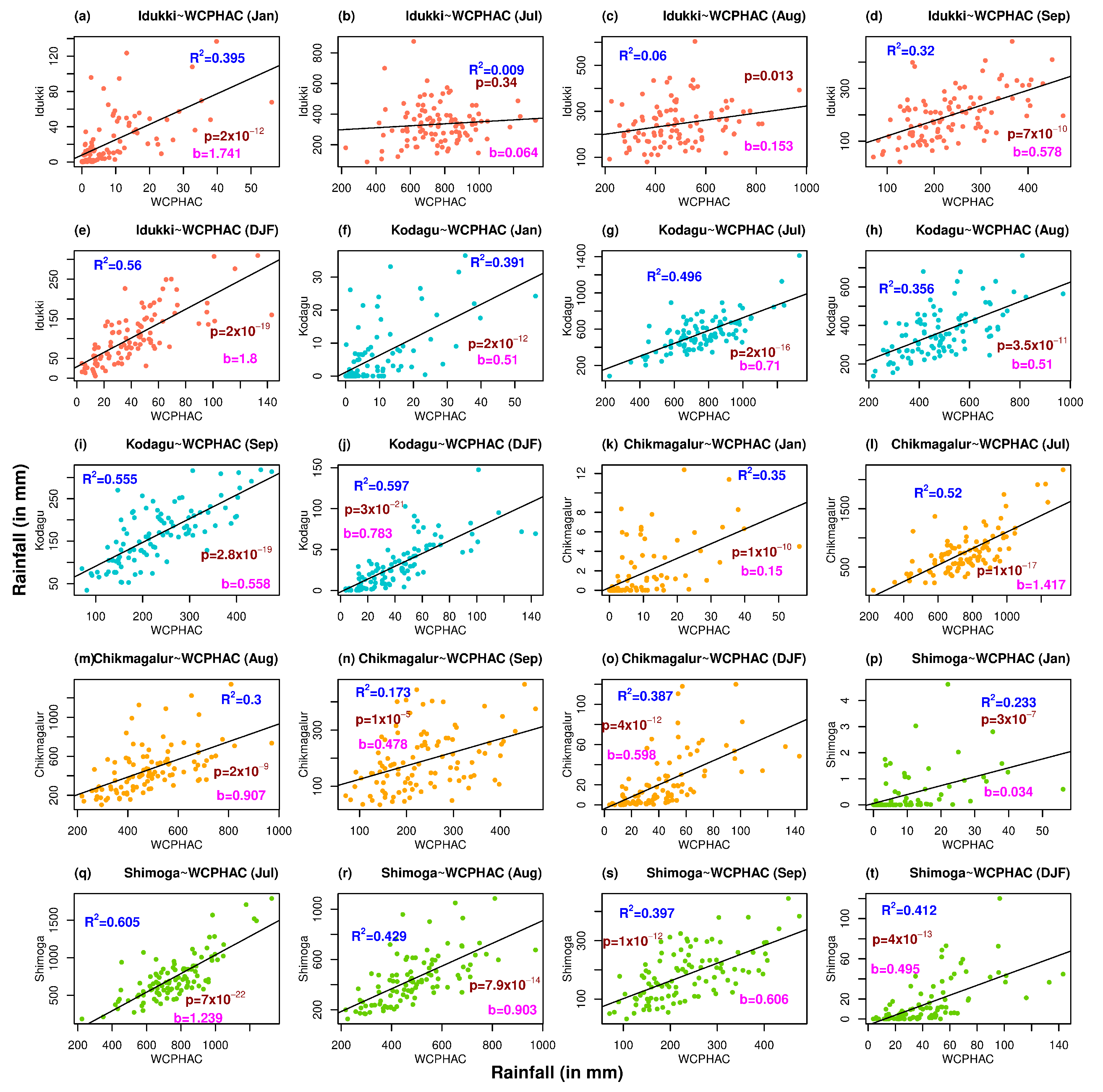
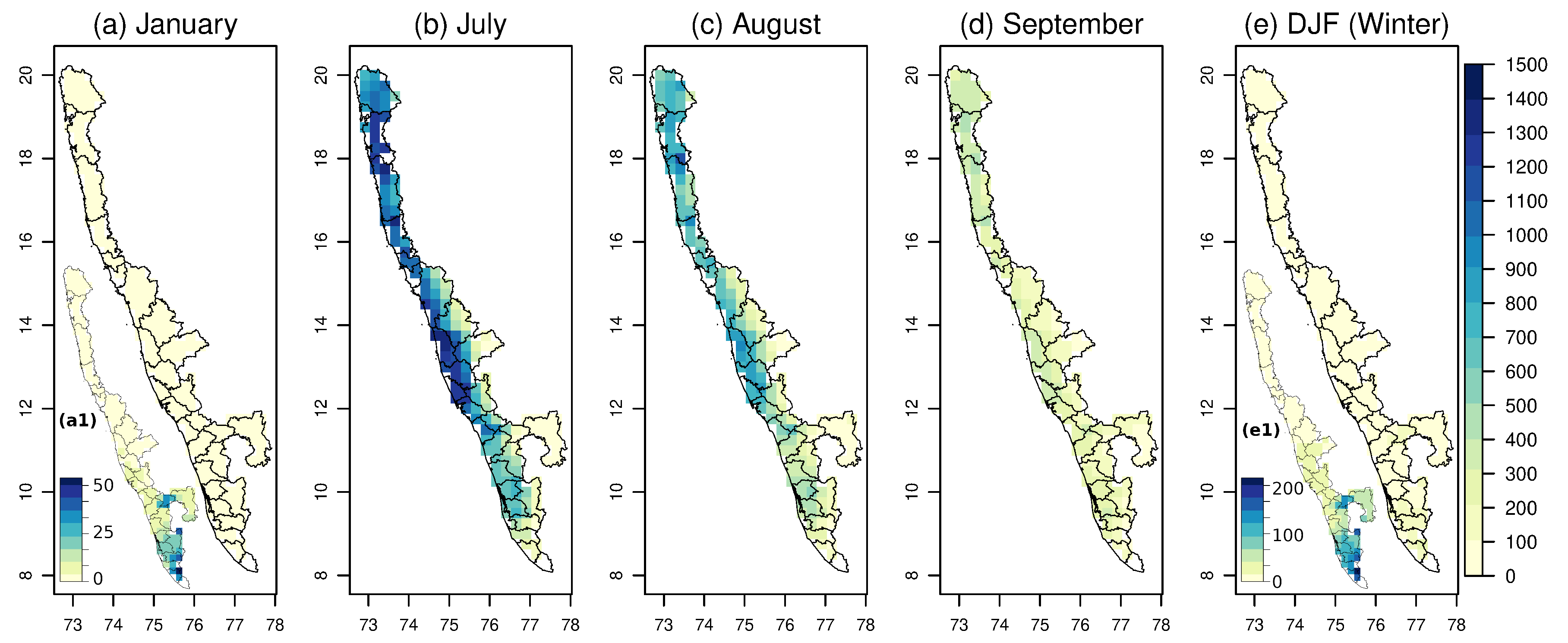
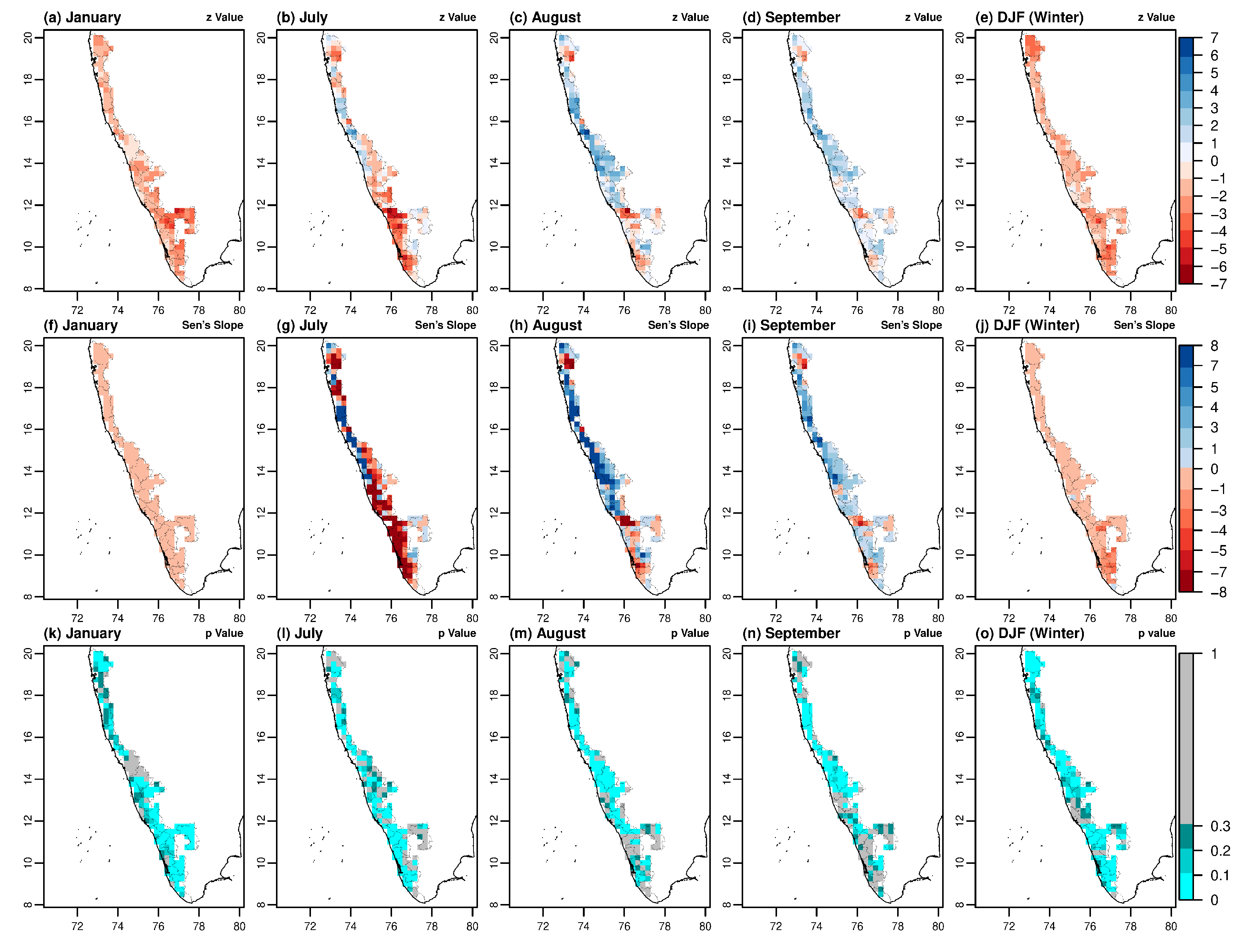
3.1. Monthly and Seasonal Analysis

Out of all the twelve months, we obtained significant results in common using MMKT and linear regression for January, July, August, and September months only (Table 2 and Table 3). Except for the Erode district, all other districts receive a nice amount of rainfall. Importantly, July, August, and September are months with a comparatively low value of disparity and the average D value calculated for the region in these three months is only 25.68%, 35.36%, and 43.60% respectively.

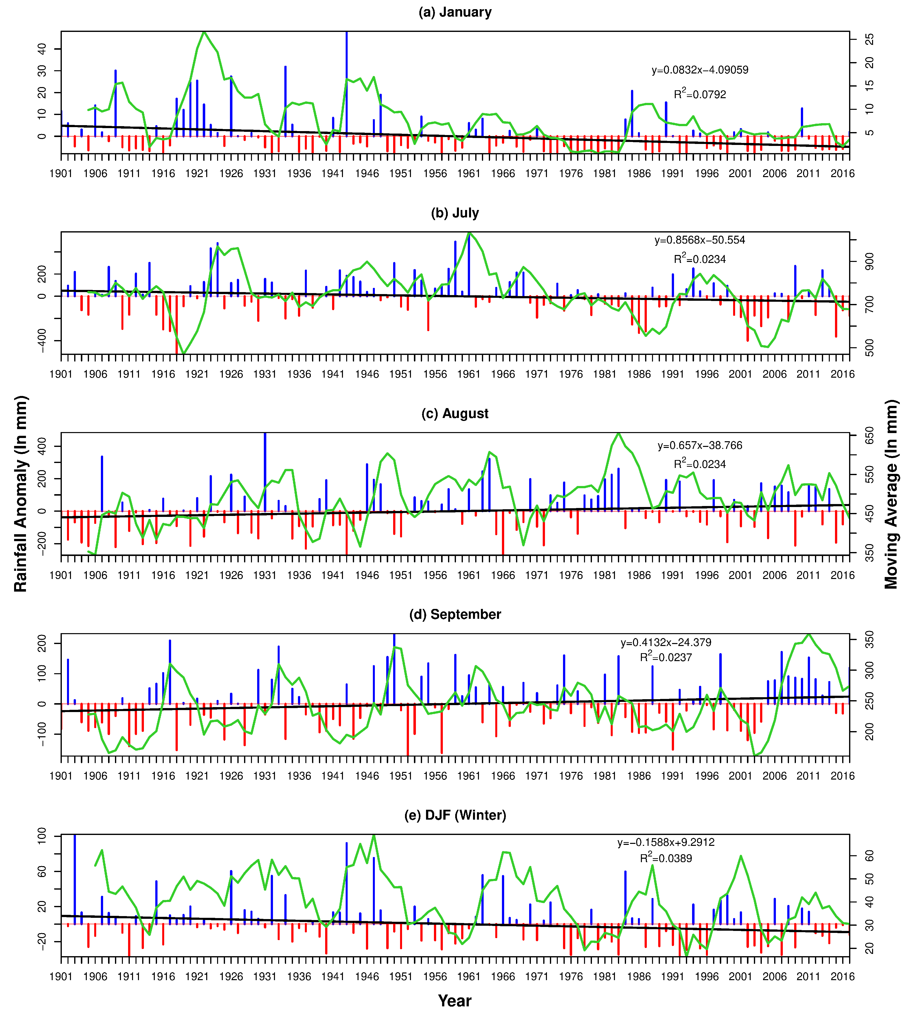
3.1.1. January and July (Monthly Negative Trend)

January has a place among low rainfall receiving months with only 0.3% contribution to the annual rainfall. Figure 3a1 shows that the distribution of rainfall ranges between 0–50 mm only and it is high in the southern part of the region. In addition to it, January is also notable with its highest D value (197.14%) compared to all the months and seasons (Table 1). The least rainfall with 75% probability is received in this month and it is a matter of concern for the southern part of the region. Already a low amount of rainfall can get diminished in the long run in the region. January dataset is found highly skewed (right-skewed) with an exceptionally high value of 1.27 and its kurtosis value represents its heavy-tailed nature (Table 2).

July month is important for the region because it contributes about 30% of the total annual rainfall (Table 1) and has a 75% chance of having more than 625 mm rainfall occurrence. The huge contribution of rainfall amount in this month is also visible in other numerical figures. It has the least D value among all the significant results (Table 1). The spatial distribution is also found equally high for the majority of the parts in the region. Exceptionally, the southern part in this month does not receive comparatively high rainfall and Varikoden et al. [19] highlighted the occurrence of such phenomena is due to the northern shift of the low-level jet stream.

January has a decreasing rainfall trend (significant at a 99% level) with linear regression and MMKT results. The right skewed nature of rainfall is also reflected in the moving average (Figure 4a). The spatial pattern of the MMKT results for January in Figure 5a shows a high z value for the Erode district and other southern parts of the region. Whereas, the magnitude of decrease in rainfall (Sen’s slope) remain homogeneous with the range of 0 to −1 mm year⁻¹ (Figure 5f). The significance level of the trend is not satisfactory for the Goa state of India and found highly significant for the southern parts of the region (Figure 5k). Results with the ITA method also show a decreasing trend with high significance for the low rainfall events (Figure 6a). A sharp decrease in the occurrence of high rainfall events can also be observed but the trend for such events is not found significant.

The second month with a decreasing trend is July and surprisingly, it is found with a very high magnitude of decreasing rainfall (Table 2 and Table 3). Only, Goa state of India and its adjacent area show a positive trend of rainfall with high magnitude (Figure 5b). Most of the parts of the region with a decreasing trend show a magnitude of more than −7.00 mm year⁻¹ (Figure 5g). Knowing that July receives more than 30% of the total annual rainfall of the year, it signals the serious concern and therefore an independent study on the atmospheric dynamics during July month will help to understand it. ITA results in Figure 6b strongly support the significant decreasing trend for almost all the rainfall events (independent of the size of rainfall events). Only very few high rainfall events are observed towards the decreasing trend region in the ITA Figure 6b.

3.1.2. August and September (Monthly Positive Trend)

The regional distribution during August shows some pockets of very high rainfall (dark blue spots) in districts around Mumbai (Figure 3c) and all across the coastal area of WCPHAC region. Figure 3d–e show more or less the homogeneous distribution of rainfall in September and Winter. Characteristics for August and September months for 117 years reflects less (more) annual contribution with the more (less) D value. Kurtosis and skewness are almost normal for these two significant months of monsoon season (Table 2).

August is the second most important month concerning a total annual contribution of 19.70% and the monotonic trend is toward the increase as shown with z-stat and ITA trend value summarized in Table 2. In 117 years period, rainfall increased with the magnitude of 0.81 mm year⁻¹ (Sen’s slope) and 0.67 mm year⁻¹ (ITA slope). This magnitude of the increase is second highest among all succeeded by September month. Skewness has been little right-skewed and kurtosis of 0.04 represents a very little bulge that is not abnormal and usually remains under the normal curve. z value for August shows the increasing trend of rainfall in the whole region except the southern part of the region (also known as Kerala) and a very small pocket in the north of the region (Figure 5c). The magnitude of rainfall increase in the coastal plain belt of the region is very high (Figure 5h) and the decreasing trend of rainfall in the southern part is moderate but the p-value shows (Figure 5m) it is not significant at the 90% level. This monotonic trend is also supported by the results of the ITA method (Table 2) and a graphical illustration of the ITA result in Figure 6c reveals the monotonic increasing trend of rainfall as the points in the plot lie above the 1:1 line of no trend. The decreasing trend is found in the high rainfall events of August.

Following the similar pattern of a monotonic increasing trend, September month has the 0.45 mm year⁻¹ (Sen’s slope) and 0.35 mm year⁻¹ (ITA slope) indicating the increasing trend in rainfall. Kurtosis value shows the distribution is not at all bulging out but have the right skewness. Spatial distributions of the MMKT z value (Figure 5d) and Sen’s slope (Figure 5i) are similar to the pattern in August but the magnitude of the September trend is a bit less intense than August month. Unfortunately, the decreasing trend of rainfall in the southern part of the region is not highly significant for September month as shown in Figure 5n. Results of the ITA method for September also favor the increase in rainfall except for the high rainfall episodes as observed in September (Figure 6d). September month observes the monsoon retreat from India and for that matter rainfall by retreating monsoon is also important concerning the general dynamics of atmospheric circulation and survival of the ecosystem in the WCPHAC region. Linear regression results in Table 3 are found in complete agreement with the magnitude and trend of rainfall in all the different significant periods in this study.

3.1.3. Winter Rainfall Trend

The Winter season has a monotonic declining rainfall trend supported by results from MMKT, linear regression as well as ITA methods. The trend line in Figure 4e shows it clearly and a five-year moving average kept on being highly fluctuating, which can be understood with 112.40% D value given in Table 1. The Winter season has a continuous declining trend, which maintained its rhythm even after the 1950s. The congestion of black bars hanging downward clearly depicts the start of the decline in rainfall in Winter (after 1970). The contribution of Winter season rainfall is 1.65% in the annual total rainfall (Table 1) and its spatial distribution in Figure 3e shows its homogeneous distribution in the whole WCPHAC region.

Among the three different periods with a significant result, the highest D value, skewness, and kurtosis lie in the Winter season (Table 1). The kurtosis value of a normal curve is normally 3 and the higher value of kurtosis than the normal curve is called a leptokurtic curve. Results obtained using MMKT and linear regression method are indicative of significant monotonic trend (Table 2 and Table 3) and both the trend analysis results with z-stat and intercept value of the linear regression equation (Table 3) agree with a monotonic decreasing trend. ITA results are also indicative of decreasing rainfall in the Winter season (Table 2). The magnitude of the decreasing trend obtained is −0.14 mm year⁻¹ (Sen’s slope) and −0.06 mm year⁻¹ (ITA slope). The magnitude is not very high though the existing decrease which is significant at 99% level cannot be ignored as the contribution of Winter season rainfall is 1.65%.

The spatial distribution of z value (Figure 5e) and its slope (Figure 5j) illustrate the decreasing trend of rainfall across the whole region. Only the southern part of the region has a comparatively higher magnitude (Figure 5i) of decrease in rainfall and here this decline in the southern part is significant at 90% level which is contrary to the trend observed for the southern part of WCPHAC region in August and September month. We found that the results of the ITA method are also showing a decreasing rainfall trend (Table 2 and Figure 6e). Whereas, some high-end rainfall episodes are observed as outliers with higher decreasing magnitude (Figure 6e).

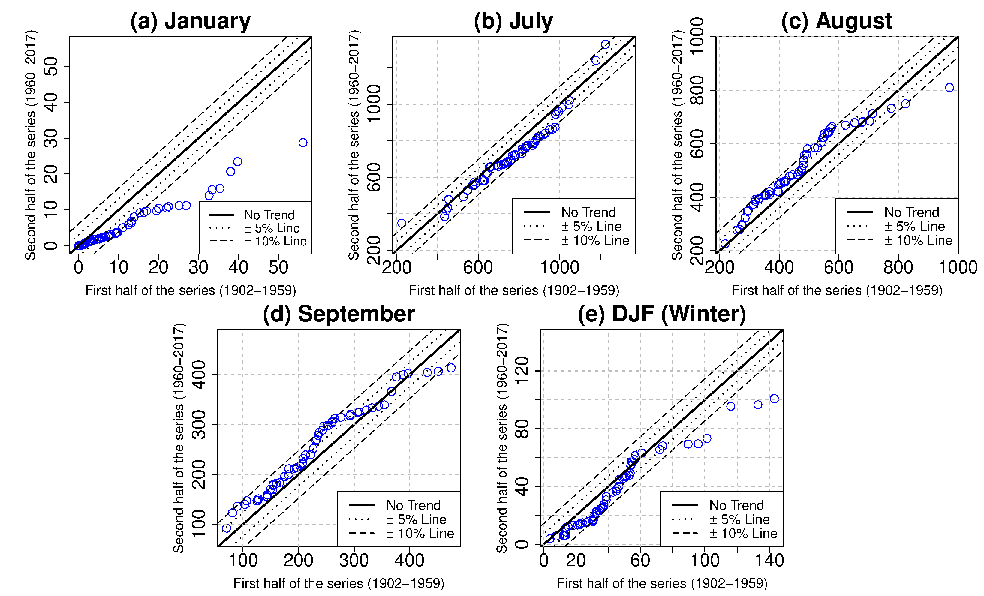
3.2. Decadal Analysis

Decadal contribution and anomaly of rainfall amount of all the months and Winter season are shown in

Table 4. Decadal anomaly percentage of rainfall and contribution of periodic rainfall with respect to the normal rainfall for the period 1901–2017.

Decade	January		July		August		September		DJF (Winter)
	Anomaly (%)	Contribution (%)	Anomaly (%)	Contribution (%)	Anomaly (%)	Contribution (%)	Anomaly (%)	Contribution (%)	Anomaly (%)	Contribution (%)
1901–1910	60.71	0.54	2.54	32.66	−12.29	18.24	−13.66	8.93	31.60	2.29
1911–1920	26.95	0.43	−12.67	27.92	−15.77	17.58	−4.82	9.88	1.09	1.77
1921–1930	86.64	0.59	11.00	33.25	−1.05	19.35	−7.04	9.04	17.97	1.93
1931–1940	−12.57	0.27	0.96	29.15	4.41	19.68	−1.31	9.25	−2.72	1.54
1941–1950	63.17	0.50	12.83	32.29	−2.42	18.23	10.58	10.27	36.15	2.13
1951–1960	−35.73	0.19	10.55	30.69	2.88	18.65	−2.88	8.75	−29.68	1.07
1961–1970	−10.59	0.28	13.14	33.63	5.69	20.51	2.89	9.93	28.03	2.08
1971–1980	−76.28	0.08	−6.14	29.05	2.16	20.64	0.38	10.08	−27.05	1.24
1981–1990	4.44	0.36	−16.14	27.15	13.97	24.08	−5.67	9.91	−6.88	1.65
1991–2000	−40.60	0.19	5.51	31.20	0.70	19.44	−3.76	9.24	−11.84	1.43
2001–2010	−30.58	0.23	−15.20	26.41	0.58	20.45	9.13	11.03	−21.72	1.33
2011–2017	−50.81	0.16	−9.09	27.98	1.64	20.41	23.09	12.29	−16.84	1.40

. The contribution of Winter rainfall was higher in the earlier decades of the study period and became almost half in recent decades. The average contribution of Winter rainfall in 1901–1950 was 1.93% which declined to an average of 1.46% in 1951–2017. The least decadal contribution in Winter is observed during 1951–1960. Since 1901, the Winter rainfall anomaly is never been in negative numbers. However, the percentage anomaly value as shown in Table 4 is decreasing over time. While considering 1901–1950 and 1951–2001, we found an increase of about 2% decadal contribution in August, 0.70% in September and a decrease of −0.25%, −1.37% and −0.48% in January, July, and Winter season respectively, which supports the trend results discussed in detail in Section 3.1.

Decadal analysis of the rainfall has also shown that since 1951–1960 decade, an average decrease of more than −34% is found in January month. Only one decade (1981–1990) with a little positive anomaly of 4% is observed. July has an average decadal decline of −8% since 1971–1980. The decade with the highest decline in January and July were 1991–2000 (−40%) and 1981–1990 (−16%) respectively. Whereas, a continuous decrease in the Winter season’s decadal rainfall is observed and it has become an almost continuous phenomena. Since 1971–1980 percentage of change in rainfall anomaly is very high in comparison to August and September besides the fact that August and September contribute 30% in annual total rainfall. On the other hand, the positive anomaly of especially August month since 1951–1960 and along with it September month have observed some minute negative anomaly in the second half of the period 1901–2017. These small values of negative anomaly percentage can be compromised with the finely maintained percent decadal contribution of September rainfall. Some similarity is observed in the changing anomaly and percent decadal contribution with the general identified significant monotonic trend of four months and a season.

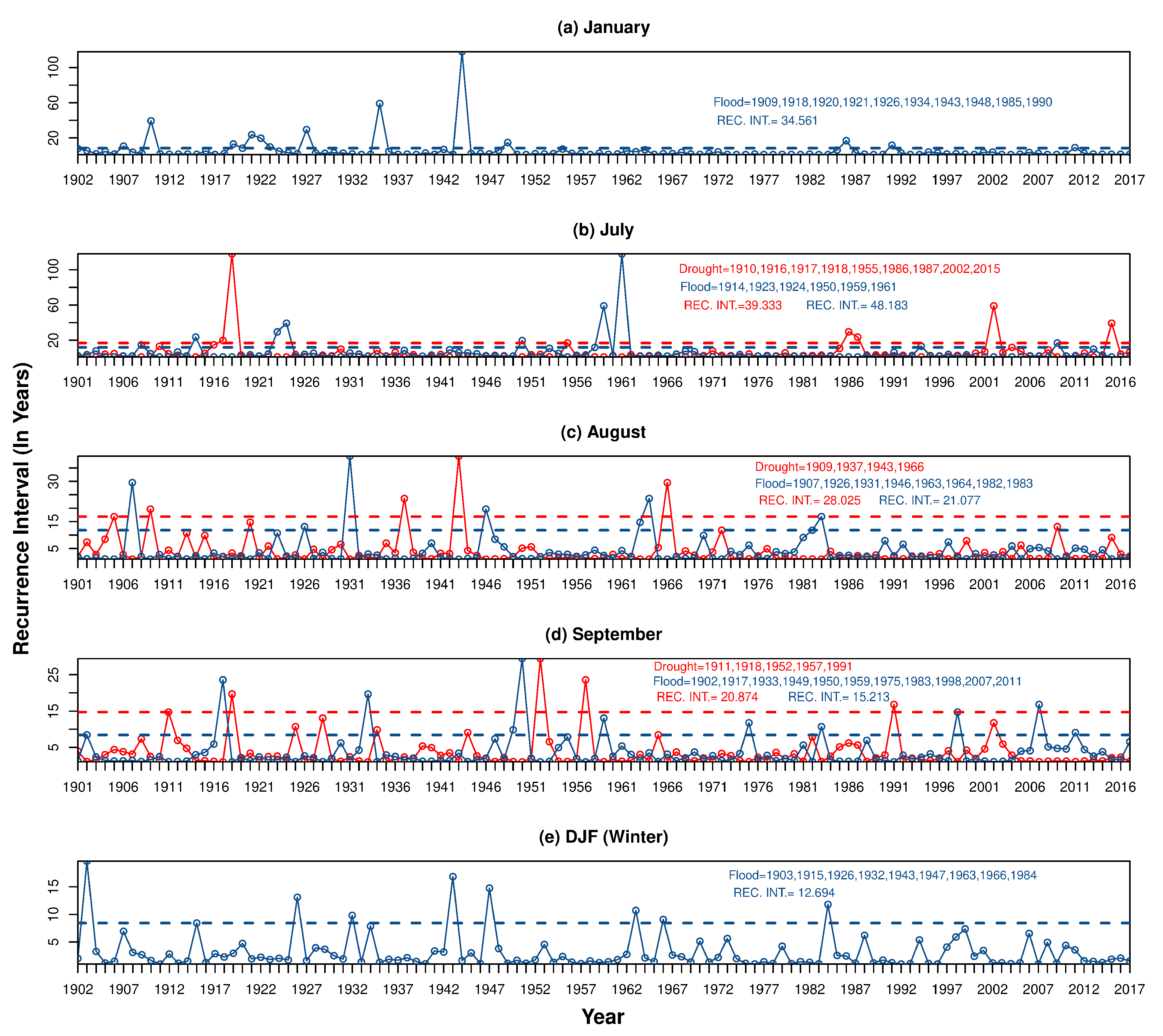
3.3. Recurrence Interval

Extreme rainfall events are the most probable cause for the highly skewed data and high kurtosis value. The existence of extreme events has been a serious concern for different regions of the world due to its devastating impact on the environment. Therefore, it has been widely studied to identify extreme events and their probable occurrence in different regions [79,80,81]. Whereas, trend results in the present study represent the existence of positive skewness and kurtosis during the period 1901–2017 and therefore we attempted here to analyze the size of extreme monthly and seasonal events of rainfall following the SD based scheme [82] with ±1.5 SD (+1.5 SD means excess/flood and −1.5 SD means deficit/drought). Among the significant declining rainfall trend, we found no deficit event in January month (Figure 7a). As far as the occurrence of the excess event is concerned, only two events after 1950 have been observed. These two in 1985 and 1990 were far below the average recurrence interval with a value of 16 and 11 years respectively. This decrease in the excess events follows a similar trend of the general decrease in rainfall of January month. July is the second month with a significant decreasing rainfall trend and it has not observed excess events after 1960 (Figure 7b). Whereas, 4 deficit events have been observed since 1960. Between 1901 to 2017, 9 were deficit and 6 were an excess event. The calculated mean value of deficit event years is very low in comparison to excess years in July and it shows comparatively high chances of drought. Overall, July has the highest value of recurrence interval for the deficit as well as the excess year and thus makes it comparatively less vulnerable to extreme events.

We found the highly crisscross pattern in the recurrence interval for August and September month (Figure 7c–d). Both types of extreme events show a decline in intensity in August month. September has an almost mixed pattern and supports the fact of very moderate positive skewness and moderate negative kurtosis. September has the least recurrence interval for the excess events and has 6 out of 11 occurrences of such events in the second half of the century. September month has observed the maximum number (11) of excess events with an average recurrence interval of 15.21 years and extreme being the year 1950 (Figure 7d). It supports the decline in the intensity of extreme events along with a general decline in the rainfall trend.

During the Winter season, there is no deficit year and have 9 excess years with an average recurrence of 12.69 years (Figure 7e). This suggests the probability of an excess year every 12.69 years. No deficit events are seen in the Winter season and there are no excess years after 1984. It should be noted here that the lower (higher) the value of recurrence interval, the higher (lower) the chances of its occurrence. The low value of recurrence interval for the Winter season indicated the probability of higher occurrence of excess events but on the other hand, a significant decline is noticed in the monotonic trend. Winter season has the highest value of D (Table 1) among all the seasons and months, whether it is significant or not. Therefore, it could be the influence of disparity over the occurrence of excess rainfall events of the season.

4. Discussion

In the obtained results with increasing (decreasing) rainfall in August and September (January, July, and Winter). July, August, and September months being part of monsoon season are important because the southwest monsoon plays a very important role in the modulation of peninsular climate and any change in the constituent months becomes very critical. The spatial distribution of rainfall showed July, August, and September receive comparatively high rainfall in the coastal plain area of the region. The decrease in July month’s rainfall is widely spread across the region. Whereas, southern part and a small pocket in the northern part faces a decrease in rainfall trend. The decrease in the rainfall trend of August and September in these specific areas of the region is certainly contrary to the trend of the whole region as a unit. The reason for such a contrasting trend as discussed by Varikoden et al. [19] is the northward movement of the low-level jet stream from 10${}^{\circ }$ N to 15${}^{\circ }$ N due to warming of the Arabian Seas and tropospheric temperature over north India. The same phenomena may also be responsible for higher z value and slope magnitude of the southern parts of the region during July month. In an earlier study, using the point data for the southern part of the WCPHAC region for the period 1871–2014, the non-monotonic decreasing rainfall trend was observed [83]. However, the grid wise analysis of the trend in the present study has revealed the significant monotonic trend for the majority of grids in the southern part of the region. The results in this study support the fact that the increase of monsoon rainfall in the northern and middle part of the region during 1871–2014 exists [83]. It is due to the observed net increasing trend in the monsoon season’s constituent months (Table 2). In another study on the southern part of the region, the significant increasing rainfall trend obtained using point data for January is not in agreement with the results obtained using grid wise analysis in the present study (Figure 5b,g,l) [84]. Whereas, the significantly decreasing trend in July is highly acceptable. Hence, using grid data for the identification of significant monotonous trend is found highly advantageous in the present study. On the other hand, considering the WCPHAC region as one unit also found important by showing the performance of the whole region with one representative value.

Changing patterns of rainfall over the region will get serious implications and one may be the decision to change the sub-region having the first onset of monsoon in India. Varikoden et al. [19] used the same dataset as used in the present study, therefore, narratives set by their study are more significant in the context of a decrease in rainfall toward the southern part and some pockets in the north of the WCPHAC region. An in-depth study as completed by Nayak and Mandal [85] will be important to understand the impact of changing land-use and land-cover in WCPHAC region’s rainfall. In the present study, we used the ITA method along with MMKT and linear regression method to have synchronized results and to have innovative graphical illustration of rainfall trend for the months and seasons with a significant trend. Finely synchronized results are obtained using all these methods except one discrepancy with the ITA method. Trend result for June month showed a decreasing trend of rainfall but MMKT and linear regression are contrary to it. However, results for June with MMKT and linear regression are found insignificant.

Other than the significant increasing trend results, the large decreasing significant trend in July is obtained and it is very critical for the region due to the large contribution of this month’s rainfall to the annual rainfall. This large amount of rainfall of July alone is almost equal to the combined total contribution of August and September in total annual rainfall.

In this study, adoption of the ITA method has been in complete agreement with the significant results obtained using MMKT and linear regression and it is also highly fruitful in the present study to know the trend of high/low rainfall events. Graphical illustration of ITA results in Figure 6a–e revealed that the trend of high rainfall amount is towards decrease though the overall trend results of ITA for July, August, September, and Winter season remained highly significant at 90% level. Therefore, we suggest that the ITA method should be used not only to find out the more accurate monotonic trend but also to have a look at the direction of the trend of events with different rainfall amounts.

5. Conclusions

This study analyzed the trend of rainfall in the WCPHAC region from 1901–2017. MMKT and linear regression analysis were used to identify the significantly monotonic monthly and seasonal trends. The purpose of the adoption of MMKT was to remove the influence of serial correlation through the variance correction approach. Decadal analysis of the rainfall was performed for January, July, August, September months and Winter season due to the obtained significant results. A rigid method to extract the monotonic trend significant at the 90% level is adopted with the application of MMKT and linear regression. The obtained results were further tested through the application of the new method of trend analysis (ITA) having certain advantages with the graphical illustration of results.

A significant monotonic decrease in rainfall was seen in January, July, and the Winter season. Whereas an increasing trend was found in August and September. Right skewness existed in almost all the significant and insignificant results. A visual analysis of the trend suggested that it was most probably due to the presence of the monthly extremes in the earlier part of the study period. Exceptionally very high right skewness and heavy tail are found in January month. In the last 50 years, many excess years were observed in August and September as compared to deficit years. This phenomena somewhat justifies the monotonic increase (decrease) in the rainfall trend of August and September (January, July, and Winter season). A comprehensive study is needed to understand that influence and the connection between general monotonic trend and excess or deficit rainfall events.

Decadal analysis to a great extent was in agreement with the identified significant monotonic rainfall trend of different months and winter season. Interestingly, no decade with a negative anomaly is seen in August for the last 67 years. These facts are of immense value for agricultural practices and forest management in the study region. We hope our analysis is helpful to improve the socio-economic conditions of the region under the changing rainfall patterns and stress of global warming.

References

1. Foster, G.L.; Royer, D.L.; Lunt, D.J. Future climate forcing potentially without precedent in the last 420 million years. Nat. Commun. 2017, 8, 1. [Google Scholar] [CrossRef] [Green Version]
2. Barnosky, A.D.; Kraatz, B.P. The Role of Climatic Change in the Evolution of Mammals. BioScience 2007, 57, 523–532. [Google Scholar] [CrossRef] [Green Version]
3. Sörlin, S.; Lane, M. Historicizing climate change-engaging new approaches to climate and history. Clim. Chang. 2018, 151, 1–13. [Google Scholar] [CrossRef] [Green Version]
4. Steffen, W.; Rockström, J.; Richardson, K.; Lenton, T.; Folke, C.; Liverman, D.; Summerhayes, C.; Barnosky, A.; Cornell, S.; Crucifix, M.; et al. Trajectories of the Earth System in the Anthropocene. Proc. Natl. Acad. Sci. USA 2018, 115, 8252–8259. [Google Scholar] [CrossRef] [Green Version]
5. Boyce, C.K.; Lee, J.E. Plant Evolution and Climate Over Geological Timescales. Annu. Rev. Earth Planet. Sci. 2017, 45, 61–87. [Google Scholar] [CrossRef]
6. Kabanda, T. Long-term rainfall trends over the Tanzania coast. Atmosphere 2018, 9, 155. [Google Scholar] [CrossRef] [Green Version]
7. Rao, V.B.; Franchito, S.H.; Santo, C.M.E.; Gan, M. An update on the rainfall characteristics of Brazil: Seasonal variations and trends in 1979–2011. Int. J. Climatol. 2016, 36, 291–302. [Google Scholar] [CrossRef]
8. Frazier, A.G.; Giambelluca, T.W. Spatial trend analysis of Hawaiian rainfall from 1920 to 2012. Int. J. Climatol. 2017, 37, 2522–2531. [Google Scholar] [CrossRef]
9. Longobardi, A.; Villani, P. Trend analysis of annual and seasonal rainfall time series in the Mediterranean area. Int. J. Climatol. 2010, 30, 1538–1546. [Google Scholar] [CrossRef]
10. Kidson, J.W.; Newell, R.E. African rainfall and its relation to the upper air circulation. Q. J. R. Meteorol. Soc. 1977, 103, 441–456. [Google Scholar] [CrossRef]
11. Sahu, N.; Behera, S.K.; Ratnam, J.V.; Silva, R.V.D.; Parhi, P.; Duan, W.; Takara, K.; Singh, R.B.; Yamagata, T. El Niño Modoki connection to extremely-low streamflow of the Paranaíba River in Brazil. Clim. Dyn. 2014, 42, 1509–1516. [Google Scholar] [CrossRef]
12. Sahu, N.; Singh, R.B.; Kumar, P.; Silva, R.V.D.; Behera, S.K. La Niña Impacts on Austral Summer Extremely HighStreamflow Events of the Paranaíba River in Brazil. Adv. Meteorol. 2013, 2013, 1–6. [Google Scholar] [CrossRef]
13. Sahu, N.; Behera, S.K.; Yamashiki, Y.; Takara, K.; Yamagata, T. IOD and ENSO impacts on the extreme stream-flows of Citarum river in Indonesia. Clim. Dyn. 2012, 39, 1673–1680. [Google Scholar] [CrossRef]
14. Rajeevan, M.; Sridhar, L. Inter-annual relationship between Atlantic sea surface temperature anomalies and Indian summer monsoon. Geophys. Res. Lett. 2008, 35, 21. [Google Scholar] [CrossRef]
15. Ashok, K.; Behera, S.K.; Rao, S.A.; Weng, H.; Yamagata, T. El Niño Modoki and its possible teleconnection. J. Geophys. Res. 2007, 112. [Google Scholar] [CrossRef]
16. Roy, I. Indian Summer Monsoon and El Niño Southern Oscillation in CMIP5 models: A few areas of agreement and disagreement. Atmosphere 2017, 8, 154. [Google Scholar] [CrossRef] [Green Version]
17. Doranalu Chandrashekar, V.; Shetty, A.; Patel G C, M. Estimation of Monsoon Seasonal Precipitation Teleconnection with El Niño-Southern Oscillation Sea Surface Temperature Indices over the Western Ghats of Karnataka. Asia-Pac. J. Atmos. Sci. 2019, 1–15. [Google Scholar] [CrossRef]
18. Manjunatha, B.; Balakrishna, K.; Krishnakumar, K.; Manjunatha, H.; Avinash, K.; Mulemane, A.; Krishna, K. Increasing Trend of Rainfall Over Agumbe, Western Ghats, India in the Scenario of Global Warming. Open Oceanogr. J. 2015, 8, 39–44. [Google Scholar] [CrossRef]
19. Varikoden, H.; Revadekar, J.V.; Kuttippurath, J.; Babu, C.A. Contrasting trends in southwest monsoon rainfall over the Western Ghats region of India. Clim. Dyn. 2019, 52, 4557–4566. [Google Scholar] [CrossRef]
20. Raj, P.P.N.; Azeez, P.A. Trend analysis of rainfall in Bharathapuzha River basin, Kerala, India. Int. J. Climatol. 2012, 32, 533–539. [Google Scholar] [CrossRef]
21. Mudbhatkal, A.; Amai, M. Regional climate trends and topographic influence over the Western Ghats catchments of India. Int. J. Climatol. 2018, 38, 2265–2279. [Google Scholar] [CrossRef]
22. Prakash, S.; Sathiyamoorthy, V.; Mahesh, C.; Gairola, R. Is summer monsoon rainfall over the west coast of India decreasing? Atmos. Sci. Lett. 2013, 14, 160–163. [Google Scholar] [CrossRef]
23. Paul, S.; Ghosh, S.; Rajendran, K.; Murtugudde, R. Moisture Supply From the Western Ghats Forests to Water Deficit East Coast of India. Geophys. Res. Lett. 2018, 45, 4337–4344. [Google Scholar] [CrossRef]
24. Zhang, G.; Smith, R.B. Numerical Study of Physical Processes Controlling Summer Precipitation over the Western Ghats Region. J. Clim. 2018, 31, 3099–3115. [Google Scholar] [CrossRef]
25. Sreelash, K.; Sharma, R.K.; Gayathri, J.A.; Upendra, B.; Maya, K.; Padmalal, D. Impact of Rainfall Variability on River Hydrology: A Case Study of Southern Western Ghats, India. J. Geol. Soc. India 2018, 92, 548–554. [Google Scholar] [CrossRef]
26. Alvi, S.M.A.; Koteshwaram, P. Time Series Analysis of Rainfall over India. MAUSAM 1985, 36, 479–490. [Google Scholar]
27. Naidu, C.V.; Durgalakshmi, K.; Krishna, K.M.; Rao, S.R.; Satyanarayana, G.C.; Lakshminarayana, P.; Rao, L.M. Is summer monsoon rainfall decreasing over India in the global warming era? J. Geophys. Res. 2009, 114. [Google Scholar] [CrossRef] [Green Version]
28. Koteswaram, P.; Alvi, S.M.A. Trends and Periodicities in Rainfall at West Coast Stations in India. Curr. Sci. 1969, 38, 229–231. [Google Scholar]
29. Daniel, B.; Darwall, W.; Molur, S.; Smith, K.C. (Eds.) The Status and Distribution of Freshwater Biodiversity in the Western Ghats, India; IUCN: Cambridge, UK; Gland, Switzerland, 2011. [Google Scholar]
30. Shrestha, D.; Deshar, R.; Nakamura, K. Characteristics of Summer Precipitation around the Western Ghats and the Myanmar West Coast. Int. J. Atmos. Sci. 2015, 2015, 1–10. [Google Scholar] [CrossRef]
31. Verma, R.R.; Manjunath, B.L.; Singh, N.P.; Kumar, A.; Asolkar, T.; Chavan, V.; Srivastava, T.K.; Singh, P. Soil mapping and delineation of management zones in the Western Ghats of coastal India. Land Degrad. Dev. 2018, 29, 4313–4322. [Google Scholar] [CrossRef]
32. Manigandan, P.K.; Chandar Shekar, B. Risk assessment of radioactivity in soils of forest and grassland ecosystems of the Western Ghats, India. Radioprotection 2015, 50, 259–264. [Google Scholar] [CrossRef]
33. Thomas, J.; Joseph, S.; Thrivikramji, K.P. Assessment of soil erosion in a tropical mountain river basin of the southern Western Ghats, India using RUSLE and GIS. Geosci. Front. 2018, 9, 893–906. [Google Scholar] [CrossRef]
34. Pandit, P.; Mangala, P.; Saini, A.; Bangotra, P.; Kumar, V.; Mehra, R.; Ghosh, D. Radiological and pollution risk assessments of terrestrial radionuclides and heavy metals in a mineralized zone of the siwalik region (India). Chemosphere 2020, 254. [Google Scholar] [CrossRef]
35. Jha, C.; Dutt, C.; Bawa, S. Deforestation and land use changes in Western Ghats, India. Curr. Sci. 2000, 79, 231–238. [Google Scholar]
36. Davidar, P.; Arjunan, M.; Mammen, P.C.; Garrigues, J.; Puyravaud, J.P.; Roessingh, K. Forest degradation in the Western Ghats biodiversity hotspot: Resource collection, livelihood concerns and sustainability. Curr. Sci. 2007, 93, 1573–1578. [Google Scholar]
37. Panda, A.; Sahu, N. Trend analysis of seasonal rainfall and temperature pattern in Kalahandi, Bolangir and Koraput districts of Odisha, India. Atmos. Sci. Lett. 2019, 20, e932. [Google Scholar] [CrossRef] [Green Version]
38. Sahu, N.; Saini, A.; Behera, S.; Sayama, T.; Nayak, S.; Sahu, L.; Duan, W.; Avtar, R.; Yamada, M.; Singh, R.B.; et al. Impact of indo-pacific climate variability on rice productivity in Bihar, India. Sustainability 2020, 12, 7023. [Google Scholar] [CrossRef]
39. Sahu, N.; Saini, A.; Behera, S.K.; Sayama, T.; Sahu, L.; Nguyen, V.T.V.; Takara, K. Why apple orchards are shifting to the higher altitudes of the Himalayas? PLoS ONE 2020, 15, e0235041. [Google Scholar] [CrossRef]
40. Duan, W.; He, B.; Sahu, N.; Luo, P.; Nover, D.; Hu, M.; Takara, K. Spatiotemporal variability of Hokkaido’s seasonal precipitation in recent decades and connection to water vapour flux. Int. J. Climatol. 2017, 37, 3660–3673. [Google Scholar] [CrossRef]
41. Yue, S.; Wang, C.Y. The Mann-Kendall test modified by effective sample size to detect trend in serially correlated hydrological series. Water Resour. Manag. 2004, 18, 201–218. [Google Scholar] [CrossRef]
42. Bayley, A.G.V.; Hammersley, J.M.; Supplement, S.; Society, S. The “Effective” Number of Independent Observations in an Autocorrelated Time Series. Suppl. J. R. Stat. Soc. 1946, 8, 184–197. [Google Scholar] [CrossRef]
43. Hamed, K.H.; Rao, R. A modified Mann-Kendall trend test for autocorrelated data. J. Hydrol. 1998, 204, 182–196. [Google Scholar] [CrossRef]
44. Khaliq, M.N.; Ouarda, T.B.M.J.; Gachon, P.; Sushama, L.; St-Hilaire, A. Identification of hydrological trends in the presence of serial and cross correlations: A review of selected methods and their application to annual flow regimes of Canadian rivers. J. Hydrol. 2009, 368, 117–130. [Google Scholar] [CrossRef]
45. Storch, H.V. Misuses of Statistical Analysis in Climate. In Analysis of Climate Variability; Springer: Berlin/Heidelberg, Germany, 1999; pp. 11–26. [Google Scholar] [CrossRef]
46. Jaiswal, R.K.; Lohani, A.K.; Tiwari, H.L. Statistical Analysis for Change Detection and Trend Assessment in Climatological Parameters. Environ. Process. 2015, 2, 729–749. [Google Scholar] [CrossRef] [Green Version]
47. Chattopadhyay, S.; Edwards, D. Long-Term Trend Analysis of Precipitation and Air Temperature for Kentucky, United States. Climate 2016, 4, 10. [Google Scholar] [CrossRef]
48. Huth, R.; Pokorn, L. Parametric versus non-parametric estimates of climatic trends. Theor. Appl. Climatol. 2004, 77, 107–112. [Google Scholar] [CrossRef]
49. Tosunoglu, F.; Kisi, O. Trend Analysis of Maximum Hydrologic Drought Variables Using Mann-Kendall and Sens Innovative Trend Method. River Research and Applications. River Res. Appl. 2016, 33, 597–610. [Google Scholar] [CrossRef]
50. Caloiero, T. Evaluation of rainfall trends in the South Island of New Zealand through the innovative trend analysis (ITA). Theor. Appl. Climatol. 2019, 139, 493–504. [Google Scholar] [CrossRef]
51. Alifujiang, Y.; Abuduwaili, J.; Maihemuti, B.; Emin, B.; Groll, M. Innovative Trend Analysis of Precipitation in the Lake Issyk-Kul Basin, Kyrgyzstan. Atmosphere 2020, 11, 332. [Google Scholar] [CrossRef] [Green Version]
52. Gedefaw, M.; Yan, D.; Wang, H.; Qin, T.; Girma, A.; Abiyu, A.; Batsuren, D. Innovative Trend Analysis of Annual and Seasonal Rainfall Variability in Amhara Regional State, Ethiopia. Atmosphere 2018, 9, 326. [Google Scholar] [CrossRef] [Green Version]
53. Meena, H.M.; Machiwal, D.; Santra, P.; Moharana, P.C.; Singh, D.V. Trends and homogeneity of monthly, seasonal, and annual rainfall over arid region of Rajasthan, India. Theor. Appl. Climatol. 2018, 136, 795–811. [Google Scholar] [CrossRef]
54. Caloiero, T.; Coscarelli, R.; Ferrari, E. Application of the Innovative Trend Analysis Method for the Trend Analysis of Rainfall Anomalies in Southern Italy. Water Resour. Manag. 2018, 32, 4971–4983. [Google Scholar] [CrossRef]
55. Wang, Y.; Xu, Y.; Tabari, H.; Wang, J.; Wang, Q.; Song, S.; Hu, Z. Innovative trend analysis of annual and seasonal rainfall in the Yangtze River Delta, eastern China. Atmos. Res. 2020, 231. [Google Scholar] [CrossRef]
56. Khanna. Agro-Climatic Regional Planning: An Overview; Planning Commission, Government of India: New Delhi, India, 1989.
57. ICAR. Agriculture Research Databook 2019; Technical report; ICAR-Indian Agricultural Statistics Research Institute: New Delhi, India, 2019. [Google Scholar]
58. Mannan, A.; Chaudhary, S.; Dhanya, C.T.; Swamy, A.K. Regionalization of rainfall characteristics in India incorporating climatic variables and using self-organizing maps. ISH J. Hydraul. Eng. 2017, 24, 147–156. [Google Scholar] [CrossRef]
59. Dash, S.K.; Mamgain, A. Changes in the Frequency of Different Categories of Temperature Extremes in India. J. Appl. Meteorol. Climatol. 2011, 50, 1842–1858. [Google Scholar] [CrossRef]
60. Pai, D.S.; Sridhar, L.; Rajeevan, M.; Sreejith, O.P.; Satbhai, N.S.; Mukhopadhyay, B. Development of a new high spatial resolution (0.25° × 0.25°) Long Period (1901–2010) daily gridded rainfall data set over India and its comparison with existing data sets over the region. MAUSAM 2014, 65, 1–18. [Google Scholar]
61. Rajeevan, M.; Bhate, J.; Kale, J.; Lal, B. A High Resolution Daily Gridded Rainfall Data for the Indian Region: Analysis of break and active monsoon spells. Curr. Sci. 2006, 91, 296–306. [Google Scholar]
62. Shepard, D.S. Computer Mapping: The SYMAP Interpolation Algorithm. In Spatial Statistics and Models; Springer: Dordrecht, The Netherlands, 1984; pp. 133–145. [Google Scholar] [CrossRef]
63. Kothawale, D.R.; Rajeevan, M. Monthly, Seasonal and Annual Rainfall Time Series for All-India, Homogeneous Regions and Meteorological Subdivisions: 1871–2016; Technical Report RR-138; Indian Institute of Tropical Meteorology: Pune, India, 2017. [Google Scholar]
64. Mann, H.B. Non-parametric tests against trend. Econometrica 1945, 13, 163–171. [Google Scholar] [CrossRef]
65. Yue, S.; Pilon, P.; Phinney, B.; Cavadias, G. The influence of autocorrelation on the ability to detect trend in hydrological series. Hydrol. Process. 2002, 16, 1807–1829. [Google Scholar] [CrossRef]
66. Rao, A.R.; Hamed, K.H.; Chen, H.L. Nonstationarities in Hydrologic and Environmental Time Series; Springer: Dordrecht, The Netherlands, 2003. [Google Scholar] [CrossRef]
67. Sen, Z. Innovative Trend Analysis Methodology. J. Hydrol. Eng. 2012, 17, 1042–1046. [Google Scholar] [CrossRef]
68. Wu, H.; Qian, H. Innovative trend analysis of annual and seasonal rainfall and extreme values in Shaanxi, China, since the 1950s. Int. J. Climatol. 2016, 37, 2582–2592. [Google Scholar] [CrossRef]
69. Sen, P.K. Estimates of the regression coefficient based on Kendall’s tau. J. Am. Stat. Assoc. 1968, 63, 1379–1389. [Google Scholar] [CrossRef]
70. Theil, H. A rank-invariant method of linear and polynomial regression analysis. Proc. R. Neth. Acad. Arts Sci. 1950, 53, 386–392. [Google Scholar]
71. Weibull, W. A statistical study of the strength of material. Ing. Vetenskaps Akad. Handl. (Stockh.) 1939, 151, 15. [Google Scholar]
72. Fernández-Martínez, M.; Vicca, S.; Janssens, I.A.; Carnicer, J.; Martín-Vide, J.; Peñuelas, J. The consecutive disparity index, D: A measure of temporal variability in ecological studies. Ecosphere 2018, 9, 12. [Google Scholar] [CrossRef] [Green Version]
73. Meseguer-Ruiz, O.; Cantos, J.O.; Sarricolea, P.; Martín-Vide, J. The temporal fractality of precipitation in mainland Spain and the Balearic Islands and its relation to other precipitation variability indices. Int. J. Climatol. 2016, 37, 849–860. [Google Scholar] [CrossRef]
74. Meseguer-Ruiz, V.; Vide, M.; Cantos, J.O.; Espinoza, P.S. La distribución espacial de la fractalidad temporal de la precipitación en la Espańa peninsular y su relación con el Índice de Concentración. Investig. Geogr. 2014, 48, 73–84. [Google Scholar] [CrossRef] [Green Version]
75. Lana, X.; Martínez, M.; Serra, C.; Burgueño, A. Spatial and temporal variability of the daily rainfall regime in Catalonia(northeastern Spain), 1950–2000. Int. J. Climatol. 2004, 24, 613–641. [Google Scholar] [CrossRef]
76. Martín-Vide, J. Notes per a la definició d’un índex de «desordre» en pluviometria. Soc. Catalana Geogr. 1986, 7, 89–96. [Google Scholar]
77. MartínVide, J. El Temps i el Clima; Departament de Medi Ambient i Rubes: Barcelona, Spain, 2002. [Google Scholar]
78. Gaston, K.J.; McArdle, B.H. The temporal variability of animal abundances: Measures, methods and patterns. Philos. Trans. R. Soc. B Biol. 1994, 345, 335–358. [Google Scholar] [CrossRef]
79. Nkrumah, F.; Vischel, T.; Panthou, G.; Klutse, N.A.B.; Adukpo, D.C.; Diedhiou, A. Recent Trends in the Daily Rainfall Regime in Southern West Africa. Atmosphere 2019, 10, 741. [Google Scholar] [CrossRef] [Green Version]
80. Saeed, F.; Haensler, A.; Weber, T.; Hagemann, S.; Jacob, D. Representation of Extreme Precipitation Events Leading to Opposite Climate Change Signals over the Congo Basin. Atmosphere 2013, 4, 254–271. [Google Scholar] [CrossRef] [Green Version]
81. Gozzo, L.; Palma, D.; Custodio, M.; Machado, J. Climatology and Trend of Severe Drought Events in the State of Sao Paulo, Brazil, during the 20th Century. Atmosphere 2019, 10, 190. [Google Scholar] [CrossRef] [Green Version]
82. Sahu, N.; Yamashiki, Y.; Behera, S.; Takara, K.; Yamagata, T. Large Impacts of Indo-Pacific Climate Modes on the Extreme Streamflows of Citarum River in Indonesia. J. Glob. Environ. Eng. 2012, 17, 1–8. [Google Scholar]
83. Revadekar, J.; Varikoden, H.; Murumkar, P.; Ahmed, S. Latitudinal variation in summer monsoon rainfall over Western Ghat of India and its association with global sea surface temperatures. Sci. Total Environ. 2018, 613–614, 88–97. [Google Scholar] [CrossRef]
84. Krishnakumar, K.; Prasada Rao, G.; Gopakumar, C. Rainfall trends in twentieth century over Kerala, India. Atmos. Environ. 2009, 43, 1940–1944. [Google Scholar] [CrossRef]
85. Nayak, S.; Mandal, M. Impact of land use and land cover changes on temperature trends over India. Land Use Policy 2019, 89, 104–238. [Google Scholar] [CrossRef]
Figure 1. (a,b) Location map of the WCPHAC region in India and peninsular India respectively. Districts used for validating the rainfall in the WCPHAC region are highlighted with red color administrative boundary in (b). (c) The altitude of the region. The name of each district in the WCPHAC region is inside the administrative boundary of each district.
Atmosphere 11 01225 g001
Figure 2. Linear tendency of district rainfall with WCPHAC region from 1902–2002. The trend in all the cases is significant at a 99% level except Figure 2b (significant at a 66% level).
Atmosphere 11 01225 g002
Figure 3. (ae) Distribution of mean total rainfall for the period 1901–2017 in different months and seasons. Among all the figures (ae), uniformity in the use of the color bar is maintained for the representation of the magnitude of the rainfall amount. Whereas, to show the spatial variation within the region, Figure 3a and Figure 3e have inset (a1) and (e1) respectively. The unit of rainfall is mm.
Atmosphere 11 01225 g003
Figure 4. (ae) Anomaly of rainfall in the WCPHAC region. Upright blue (hanging red) bars in the figure represent positive (negative) anomaly and the black color solid line is the linear regression line of the rainfall trend. Here, the green solid line is indicative of 5 years moving average of the rainfall.
Atmosphere 11 01225 g004
Figure 5. Spatial distribution of MMKT z value (ae), Sen’s slope value (fj) and p-value in (ko) showing significance level of the result shown in (ae) and (fj). MMKT z value is in mm and unit of Sen’s slope value is mm year−1.
Atmosphere 11 01225 g005
Figure 6. (ae) Results of ITA method for (a) January, (b) July, (c) August, (d) September, and (e) Winter. X and Y-axis of the figure are representing the rainfall (in mm) for the first and second half of the whole period 1901–2017. The first half is selected as 1902–1959 by following the set convention for the case of an odd number of data points in the time series [52].
Atmosphere 11 01225 g006
Figure 7. (ae) Recurrence interval trend of the excess (+1.5 SD) and deficit (−1.5 SD) rainfall periodic events for the period 1901–2017. The blue solid line with the blue circular mark (red solid line with red circular mark) represents the recurrence interval of the excess (deficit) periodic events. Dashed blue (red) line, parallel to the x-axis marks the limit of +1.5 SD (−1.5 SD). The trend shown here is significant at a 90% level and the circular mark on the recurrence interval trend line represent the exact point of the year on the x-axis.
Atmosphere 11 01225 g007