The Significance of Fast Radiative Transfer for Hyperspectral SWIR XCO₂ Retrievals

Abstract

Fast radiative transfer (RT) methods are commonplace in most algorithms which retrieve the column-averaged dry-mole fraction of carbon dioxide (XCO${}_2$) in the Earth’s atmosphere. These methods are required to keep the computational effort at a manageable level and to allow for operational processing of tens of thousands of measurements per day. Without utilizing any fast RT method, the involved computation times would be one to two orders of magnitude larger. In this study, we investigate three established methods within the same retrieval algorithm, and for the first time, analyze the impact of the fast RT method while keeping every other aspect of the algorithm the same. We perform XCO${}_2$ retrievals on measurements from the OCO-2 instrument and apply quality filters and parametric bias correction. We find that the central 50% of scene-by-scene differences in XCO${}_2$ between retrieval sets, after threshold filtering and bias correction, that use different fast RT methods, are less than 0.40 ppm for land scenes, and less than 0.11 ppm for ocean scenes. Significant regional differences larger than 0.3 ppm are observed and further studies with larger samples and regional-scale subsets need to be undertaken to fully understand the impact on applications that utilize space-based XCO${}_2$.

1. Introduction

As of late 2020, several space-based missions are in operation with the goal to quantify the concentration of carbon dioxide (CO${}_2$) in Earth’s atmosphere. These satellites are placed in sun-synchronous low-Earth orbits and carry spectrometers with high spectral resolution to measure reflected and backscattered spectra in the shortwave infrared (SWIR) wavelength region. The currently operating instruments are GOSAT [1], launched in early 2009, OCO-2, launched in 2014, TanSat, launched in 2016, GOSAT-2, launched in 2018 and most recently OCO-3 [2] which was launched in May 2019 and installed on the International Space Station. These five instruments share the same overall concept, which is based on the measurement of two CO${}_2$ absorption bands in the SWIR near 1.6 $\mathsf{\mu }$m and 2.06 $\mathsf{\mu }$m along with the oxygen A-band at 0.756 $\mathsf{\mu }$m which can be used to constrain the reference oxygen column. While there are several other space-based instruments which obtain CO${}_2$ absorption spectra in the thermal infrared region (TIR), such as Infrared Atmospheric Sounding Interferometer (IASI), we focus only on measurements from the SWIR and relevant instruments. SWIR measurements have sensitivity to the total CO${}_2$ column down to the surface, whereas TIR measurement sensitivity is peaked at the middle and upper troposphere [3,4]. Both GOSAT and GOSAT-2 feature Fourier transform spectrometers (TANSO-FTS and TANSO-FTS-2) that point to specific locations for each single measurement. In contrast, the TanSat and OCO-2/3 instruments are grating-type spectrometers which sample the atmosphere in a push-broom manner with a small swath width of the order of 10 km. The two different instrument types have a direct impact on sampling density and total number of measurements collected in any given time range. For GOSAT [5] and GOSAT-2 [6,7], the integration time of the two FTS instruments is about the same with 4 s for each measurement scene. OCO-2/3 and TanSat, on the other hand, collect 24 and 27 measurements per second respectively. While these satellites orbit Earth around 15 times per day, the instruments collect between ∼${10}^4$ (GOSAT) and ∼${10}^6$ (OCO-2) measurements on the sunlit side of the Earth. Generally, between a third and half of those measurements remain after screening for clouds. Routine data operations for OCO-2 involve running the retrieval algorithm on the order of 60,000 of the clearest selected scenes for every day. Future CO${}_2$-focused missions push that number even further up. The geostationary Carbon Cycle Observatory [8], GeoCarb, is expected to measure well over a million cloud-free scenes over the Americas every day. The proposed CO2M mission [9] will feature a constellation of at least three satellites and a larger measurement count than GeoCarb. The computational resources to process these measurements for operational services have thus required a significant increase and will continue to do so.

The retrieval algorithms are designed to extract the column-averaged dry-air volume mixing ratio of carbon dioxide (XCO${}_2$) using mostly a three-band approach. The two CO${}_2$ absorption bands contain information on the column of carbon dioxide, whereas the O${}_2$ A-band provides a reference for the total amount of dry air within the column of a particular measurement. Having two CO${}_2$ bands separated by ∼0.4 $\mathsf{\mu }$m in wavelength in conjunction with the O${}_2$ A-band also allows to partially account for scattering by aerosols. While there is more than one degree of freedom contained in the retrieved CO${}_2$ profiles that can be exploited for explicit profile information, as was done by e.g., Kulawik et al. [10] and Noël et al. [11], most publicized data products based on SWIR-measurements collapse the profile into a column average. Other instruments allow for different approaches that retain more of the vertical information. The Atmospheric Chemistry Experiment (ACE), for example, achieves this through solar occultation measurements [12]. Other instruments, such as IASI, have a different vertical sensitivity due to the spectral location of measured absorption bands in the TIR. Crevoisier et al. [13], for example, retrieved the upper tropospheric part of the CO${}_2$ column between 11 km and 15 km using absorption bands at wavelengths 4.3 $\mathsf{\mu }$m and 15 $\mathsf{\mu }$m.

XCO${}_2$ retrievals are exceptionally challenging due to the imposed limits on systematic biases. Since one of the main applications of space-based XCO${}_2$ is the estimation of surface carbon fluxes [14], systematic biases in the XCO${}_2$ values can result in biases in the inferred surface fluxes. Chevallier et al. [15] have investigated the sensitivity of their flux inversion system and found that systematic biases on the order of ∼0.3 ppm can significantly alter the inferred surface fluxes. In order to both retain a significant number of measurement scenes as well as improve on the systematic biases, multiple scattering has to be included in the radiative transfer calculations of the retrieval forward model [16,17,18,19,20,21]. While e.g., Nelson et al. [22] have explored the possibility of applying a clear-sky only retrieval, in which atmospheric scattering is not considered, they found that scene selection and post-retrieval filtering must be performed much more aggressively to keep retrieval errors low. As such, the preferred option at the time being is to include atmospheric scattering in contemporary XCO${}_2$ retrieval algorithms, such as RemoTeC [23], the University of Leicester (UoL) algorithm [24,25], the NIES algorithm [26], WMF-DOAS [27,28], FOCAL [29,30], and the NASA Atmospheric CO${}_2$ Observations from Space (ACOS) algorithm [31].

Radiative transfer (RT) calculations are a significant computational burden on most retrieval algorithms when they include atmospheric scattering. Additionally, retrieval algorithms do not just require the calculated top-of-the-atmosphere (TOA) radiances, but also first-order derivatives of said TOA radiances with respect to various atmospheric or surface parameters, also called weighting functions. Having to compute these derivatives adds additional computational cost. Performing multiple scattering (MS) TOA radiance calculations in a purely monochromatic fashion would cause the total duration for a single retrieval to be several hours, which would make routine data operations prohibitively expensive and slow. The aforementioned retrieval algorithms thus employ so-called fast RT acceleration methods to obtain speed-ups of around two orders of magnitude to reduce the computation time for single retrievals down to merely a few minutes. In this work we focus on three specific acceleration techniques that are routinely employed by the following algorithms: RemoTeC uses linear-k [32], UoL uses a principal component-based method [33], and ACOS uses low-streams interpolation [34].

For the first time, we present a direct comparison of these three acceleration techniques in a like-for-like manner using XCO${}_2$ retrievals from OCO-2 measurements. All three fast RT methods were implemented into the UoL retrieval algorithm in a unified manner, such that the only difference is the fast RT method itself, with all other parameters and retrieval inputs being the same. Previously, Connor et al. [35] conducted a study to investigate various forward model errors in OCO-2 XCO${}_2$ retrievals, but did not include the impact of radiative transfer itself. Our work is therefore the first to attempt to quantify forward model errors in retrieved XCO${}_2$ due to radiative transfer acceleration techniques using the same retrieval algorithm.

2. Materials and Methods

2.1. The UoL Algorithm

The UoL algorithm was previously described by Cogan et al. [24], Yang et al. [25], Somkuti [36], however we summarize the main aspects that are of relevance to this work. Very similar to the ACOS and RemoTeC algorithms, the UoL algorithm considers a model atmosphere of horizontally stratified layers in which all physical properties, such as temperature and humidity, are homogeneous within each layer. Layers themselves are bounded by levels that are defined at fixed pressure values. The pressure level grid is dynamically generated for every individual scene: the first five levels are defined at 10 Pa, 100 Pa, 1000 Pa, 5000 Pa and 8000 Pa. The sixth level is set halfway between 8000 Pa and the tropopause, as obtained through the formula by Reichler et al. [37], and the seventh level is the tropopause pressure itself. The remaining 13 levels are linearly spaced between the tropopause pressure and the surface pressure. Rather than using the standard UoL processing chain for the we take the meteorological data [38] directly from the operational OCO-2 processing stream and sample them at the aforementioned pressure levels. Atmospheric CO${}_2$ fields, used as prior profiles, are taken from the General Circulation Model of Laboratoire de Meteorologie Dynamique (LMDZ) [39]. We use a Lambertian surface model for both land and ocean scenes, and prior values are estimated using the observed continuum radiance in each of the three bands.

The main retrieval set-up remains similar to other UoL data products, such as the UoL full-physics XCO${}_2$ and XCH${}_4$ products [40], or the UoL Proxy XCH${}_4$ product [41,42]. We retrieve a CO${}_2$ profile along with a temperature profile offset (additive value applied to the full temperature profile), a water vapor profile scaling factor, surface pressure, three surface albedo polynomial coefficients (quadratic), two coefficients for wavelength dispersion (linear), and finally two coefficients (scale and slope) for solar-induced chlorophyll fluorescence for land scenes. When the surface pressure changes during the retrieval, the new surface-level value of the atmospheric profiles (gases, temperature) is obtained through linear interpolation. Additionally, we also retrieve three coefficients for empirical orthogonal functions (EOFs) which are added to the final convolved modelled spectra (see O’Dell et al. [31] for details) in order to reduce spectral residuals coming mainly from spectroscopy uncertainties. We have derived the EOFs from a separate set of retrievals and use the same EOFs, regardless of the chosen fast RT method. The EOF shapes mainly reflect errors in the spectroscopic tables and the specific implementation in the gas optical property calculations. We thus do not expect them to vary significantly between the three fast RT models. Lastly, we retrieve four different aerosol types: a tropospheric fine mode, a tropospheric large mode, a cirrus cloud aerosol as well as a stratospheric sulphate-type aerosol. The cirrus cloud aerosol is initialized with a fixed optical depth of 0.005, and the altitude and width are derived from a latitude-dependent climatology [43]. The stratospheric sulphate-type aerosol is equally initialized with a fixed prior optical depth of 0.005, however at a higher altitude of 20 km. O’Dell et al. [31] point out that the stratospheric aerosol layer was introduced in V8 of the OCO-2 data product to compensate for a systematic bias in ocean glint retrievals in lower southern latitudes. The two tropospheric aerosol priors are calculated using model fields from the Copernicus Atmosphere Monitoring Service (CAMS). We group the eleven aerosol species into a fine and a large mode. The fine mode consists of one sea salt size bin (0.03 $\mathsf{\mu }$m $\le r_{\mathrm{eff}}\le$ 0.05 $\mathsf{\mu }$m), sulphates, organic matter and black carbon. The large mode contains the two other sea salt size bins (0.05 $\mathsf{\mu }$m $\le r_{\mathrm{eff}}\le$ 5 $\mathsf{\mu }$m, 5 $\mathsf{\mu }$m $\le r_{\mathrm{eff}}\le$ 20 $\mathsf{\mu }$m) as well as the two larger mineral dust size bins (0.55 $\mathsf{\mu }$m $\le r_{\mathrm{eff}}\le$ 0.9 $\mathsf{\mu }$m, 0.9 $\mathsf{\mu }$m $\le r_{\mathrm{eff}}\le$ 20 $\mathsf{\mu }$m). The smaller mineral dust size bin (0.03 $\mathsf{\mu }$m $\le r_{\mathrm{eff}}\le$ 0.55 $\mathsf{\mu }$m) is split into the fine and large modes. We retrieve a full extinction profile for each of the four aerosol mixtures, where the prior covariance matrices with nonzero off-diagonal elements restrict the actual degrees of freedom to less than ∼2. Contrary to Wu et al. [44], we do not fit a zero-level offset in any of the three bands.

The retrieval uses a nonlinear Levenberg-Marquardt type minimization technique inside an optimal estimation framework described in detail in Rodgers [45]. In this current setup, we set the Levenberg-Marquardt parameter to a higher initial value of $\gamma =500$. We made this change as the convergence of retrievals improved significantly, compared to the value of $\gamma =10$ which is used for UoL GOSAT XCO${}_2$ retrievals.

2.2. Fast Radiative Transfer

In the context of trace gas retrievals, fast radiative transfer methods aim to reduce the computational effort involved in calculating top-of-atmosphere radiances and weighting functions. One can generally think of two broad categories: one way of achieving that reduction in computational effort is to fundamentally change the way how radiances and weighting functions are calculated. The other way involves strategies that lead to a reduction of the amount of calculations that are required to obtain a full-resolution TOA spectrum as well as the related weighting functions. The work of Reuter et al. [29,30] is a recent example of the former category. Their so-called FOCAL forward model utilizes a radiative transfer scheme that involves a single scattering layer, however does not require solving the full radiative transfer equation including multiple scattering. The fast RT methods in our study fall into the latter category, being methods that reduce the number of high-accuracy RT calculations and then apply some form of interpolation or up-scaling to obtain the results for every spectral point. One main advantage of the methods compared to e.g., FOCAL is the fact that they do not require any change to the forward model itself. Using FOCAL would require a change in the setup of the model atmosphere, which would make comparisons more difficult.

The UoL algorithm uses three radiative transfer models. Scalar single scattering and polarized second orders of scattering calculations are performed using the model of Natraj and Spurr [46] (2OS). Scalar multiple scattering portions of the radiances and weighting functions are calculated using either the LIDORT model [47], or the dedicated two-stream solver (TWOSTR) [48] if the number of quadratures is exactly two. Both LIDORT and TWOSTR are radiative transfer solves which utilize the discrete-ordinates method. The number of discrete ordinates, often referred to as “streams” ($N_{\mathrm{stream}}$), is a free parameter that can be used to control the accuracy of the calculation. Higher values produce more accurate results at the cost of computation time.

The I, Q and U components of the TOA Stokes vector are calculated in the UoL algorithm as follows:

$$\left(\begin{array}{c}I\\ Q\\ U\end{array}\right)=\underset{\mathrm{LIDORT},\mathrm{TWOSTR}}{\underbrace{\left(\begin{array}{c}{I}_{\mathrm{MS}}\\ 0\\ 0\end{array}\right)}}+\underset{2\mathrm{OS}}{\underbrace{\left(\begin{array}{c}{I}_{\mathrm{SS}}+I_{\mathrm{corr}}\\ Q_{2\mathrm{OS}}\\ U_{2\mathrm{OS}}\end{array}\right)}}.$$

(1)

$I_{\mathrm{MS}}$ is the multiple-scattering, or, diffuse contribution to the total radiance, calculated either by LIDORT or TWOSTR. $I_{\mathrm{SS}}$ is the single-scatter contribution, whereas $I_{\mathrm{corr}}$ is the contribution to the single-scatter intensity due to polarization. $Q_{2\mathrm{OS}}$ and $U_{2\mathrm{OS}}$ are then the Q and U components of the Stokes vector, calculated by 2OS as well.

In the following sections, the various acceleration techniques used in this study are quickly introduced, however the reader is encouraged to consult the corresponding publications which describe the technical details of each method. The fast RT methods described below, as implemented in the UoL algorithm, use same three underlying RT codes mentioned above (2OS, TWOSTR, LIDORT).

2.2.1. Low-Streams Interpolation (LSI)

The method introduced by O’Dell [34] is an acceleration technique which shares some fundamental aspects with the correlated-k method first described by Ambartzumian [49]. LSI makes a distinction between a low-stream calculation, and a high-stream calculation and refers to MS calculations in which the number of discrete ordinates ($N_{\mathrm{stream}}$) is chosen to be either a low or a high value. Analyzing the difference between a low-stream and a high-stream calculation, one finds that it is a smooth function of the total column gas optical depth ${\tau }_{\mathrm{gas}}$. The main LSI strategy is therefore to use a handful of high-stream calculations at some chosen intervals of ${\tau }_{\mathrm{gas}}$ and use the results of those calculations to interpolate the TOA radiances and weighting functions at any ${\tau }_{\mathrm{gas}}$. O’Dell [34] found that this basic concept requires the introduction of a second dimension in addition to ${\tau }_{\mathrm{gas}}$ to account for differently shaped gas absorption profiles, especially for spectral bands which include more than one absorbing gas. LSI also features a separate calculation to account for the spectrally varying aerosol scattering and surface properties, without which the reconstructed radiances and weighting functions would feature a prominent residual slope.

In practice, the LSI technique is applied in the following manner. Given any retrieval window, the regular line-by-line RT calculations are performed using a low number of streams (e.g., 2) for the multiple-scattering RT model. Then, for a set of boundaries in ${\tau }_{\mathrm{gas}}$-space, spectral points are collected and a mean atmosphere is constructed to represent the gas and aerosol profiles of those spectral points within a bin. Then, the RT calculations are performed for both a low and high value (e.g., 16) of $N_{\mathrm{stream}}$ for the multiple-scatter contributions. Using those binned calculations, an interpolation scheme is applied to correct the line-by-line calculations that were originally performed for a low value of $N_{\mathrm{stream}}$.

The reduction in computational effort is achieved by having reduced the number of MS calculations with a large value of $N_{\mathrm{stream}}$, and the speed-up of LSI is mainly determined by how fast the low-stream calculations can be performed compared to the high-stream ones, as well as the number of chosen bins in ${\tau }_{\mathrm{gas}}$-space. Using the dedicated TWOSTR solver for the low-stream calculations improves the performance gain, compared to running the more general LIDORT solver with $N_{\mathrm{stream}}=2$.

O’Dell [34] state the relative root-mean-square errors of the LSI method radiances for various example cases using GOSAT instrument specifications. The errors generally grow with increasing solar zenith angle as well as total cloud and aerosol optical depth, and range from 0.003% (weak CO${}_2$ band, nadir, thin water cloud scenario) to 0.420% (O${}_2$ A-band, glint, multi-layer clouds plus thin near-surface aerosol).

2.2.2. Principal Component-Based Method (PCA)

The principal component-based method (PCA) was first independently described by Natraj et al. [50] and Liu et al. [51], and subsequently extended by Somkuti et al. [33]. At its core, the PCA-based method is very similar to LSI. Full line-by-line low-stream calculations are upscaled to high-stream calculations using the results of a handful of “binned” calculations. As with LSI, the speed-up is achieved via the reduction of high-stream MS calculations. The binned calculations, however, as well as the upscaling or interpolation part, are different in detail.

Similar to LSI, spectral points are first collected into bins that are separated in ${\tau }_{\mathrm{gas}}$-space. For each bin, a so-called optical property matrix is constructed, which holds all relevant per-wavelength profile information that is required to construct the full atmospheric profiles for every spectral point. The optical property matrix is then decomposed using principal component analysis. Using those principal components, we can not only reconstruct the mean binned atmospheric profile, but also a number of perturbed atmospheric states. The crucial difference between LSI and the PCA-based method is the usage of the perturbed atmospheric states which allow for a better reconstruction for spectral points that diverge from the mean atmospheric state. The number of principal components, $N_{\mathrm{EOF}}$, therefore is a free parameter that allows controlling the reconstruction accuracy, in addition to the number of ${\tau }_{\mathrm{gas}}$ bins.

In contrast to both LSI and linear-k, the PCA-based method does not introduce any explicit way of accounting for either vertical absorption structure or wavelength-dependent optical properties. Instead, both phenomena are implicitly taken into account through the principal component analysis of the optical state matrix. We also want to note that the optical state matrix as described in Somkuti et al. [33] is only one possible way of utilizing the PCA-based method. Depending on the inputs of the forward model, the contents of the optical state matrix can vary to feature more or less elements.

For the retrievals discussed in this publication, we used two different values of $N_{\mathrm{EOF}}$: one and five, and the retrieval sets are labelled PCA (1) and PCA (5), respectively. Somkuti et al. [33] quantify the radiance errors for a large ensemble of GOSAT scenes. They find that the reconstruction accuracy depends on the number of principal components (PC), as per design. Increasing the number of used PCs from one to two reduces the relative radiance errors by an order of magnitude. For two PCs, the relative radiances errors are stated to be on the order of less than 0.001% for the weak CO${}_2$ band over land, and up to 0.01% for the O${}_2$ A-band for ocean scenes.

2.2.3. Linear-k

The linear-k method, described in Hasekamp and Butz [32], follows a different strategy by omitting the low-accuracy multiple-scattering calculations altogether. Single-scatter contributions, like in LSI and the PCA-based method, are calculated exactly for every spectral point in a given retrieval band. Multiple-scattering contributions, however, are only calculated for binned atmospheric profiles. Derivatives from those binned calculations are then used to obtain the multiple-scattering radiances for all spectral points. Due to most RT models not providing second-order derivatives, the surface and atmospheric weighting functions have to be calculated through interpolation from the binned calculations. Like LSI, linear-k uses an explicit formulation to account for the vertical structure of gas absorption profiles. In our implementation, we use 15 bins that are equally spaced in $log{\tau }_{\mathrm{abs}}$-space, where ${\tau }_{\mathrm{abs}}$ is the total column optical depth due to absorption of gases and aerosols. Another difference in the UoL-implementation, compared to how the method is outlined in Hasekamp and Butz [32], is that the partial derivative with respect to the scattering optical depth is calculated using finite differences. This effectively doubles the number of the high-accuracy multiple scattering calculations to 30 per band.

The radiance errors induced by the linear-k method were explored by Hasekamp and Butz [32] for two cases. They state that the radiance residual errors are well below 0.1% for the low-aerosol case in the O${}_2$ A-band for an OCO-type instrument configuration. The error increases to up to 0.4% for a high-aerosol case.

Compared to the other two methods, the potential speed-up using the linear-k method is significantly larger due to omitting the line-by-line multiple-scattering calculations. For a typical XCO${}_2$ retrieval using the UoL algorithm (using either LSI or PCA), roughly half of the CPU time is spent in the TWOSTR model, which is used to calculate the low-stream line-by-line MS contributions.

2.3. XCO${}_2$ Retrievals from OCO-2

We processed a subset of OCO-2 scenes, using calibrated, geolocated radiances version V8r [52] from May 2016 with all three fast RT methods mentioned in Section 2.2. Due to limited computational resources, we reduced the scenes in the following way. First, we skip all scenes from even-numbered days in May 2016. Then, we remove all scenes that were taken in either target or transitional observation modes, as well as all scenes that do not have a land fraction of either 0% or 100%. Additionally, we require all scenes to have a signal-to-noise ratio of at least 100 in all three bands. This subset consists of ∼35,000 ocean glint, ∼46,000 land glint, and ∼42,000 land nadir scenes, with all eight footprints being roughly equally represented (∼15,000 to ∼16,000 each). The sensor (or viewing) zenith angles for the glint observing geometry is usually between ∼${14}^{\circ }$ and ∼${47}^{\circ }$, and nadir sensor zenith angles are mostly between $0^{\circ }$ and ∼${0.6}^{\circ }$.

The subset was chosen to be balanced between both a sufficient scene yield and to span a wider space of relevant geophysical parameters. Our scene selection was performed with OCO-2 lite files version V8r, using all warn levels. The warn level system used in the V8r version of the OCO-2 lite files was designed to facilitate a simple way for users to select XCO${}_2$ retrievals based on their individual requirements for data scatter and throughput [53]. Starting from warn level 0, which contains the “best” scenes in a given day in terms of scatter, each subsequent warn level adds more scenes and thus also increases XCO${}_2$ scatter. The warn level classification is inherently tied to geophysical parameters such as aerosols, surface roughness or the scene solar zenith angle. Thus, selecting only the scenes with the lower warn levels would significantly bias the subset towards clear scenes with very low aerosols. Since we are not using the ACOS algorithm, the warn level assignment does not fully translate to the UoL algorithm since many of the atmospheric inputs (most importantly, aerosols) are different. Using the subset described here, however, yields a solid set of cloud-free scenes with sufficient signal-to-noise ratio and a significant coverage of the crucial geophysical parameters to analyze the performance of the three fast RT methods.

Figure 1 shows the geographical distribution of the used scenes as well as their observation modes. Note that since release V9(r) [54], warn levels are no longer reported in the product files.

2.4. Filtering and Bias Correction

We treat each of the four sets of retrievals individually, meaning that we apply a new set of filters and derive separate bias correction formulations for each set. As a first step, we determine the so-called footprint bias. The underlying assumption is that the XCO${}_2$ across a full OCO-2 frame should, on average, be the same, and any systematic difference of one footprint to another one is an un-physical bias. This footprint bias is determined by collecting all retrievals for which all eight footprints of the same frame converged successfully, and compute the median XCO${}_2$ across each of those frames. The difference between each individual footprint XCO${}_2$ and the frame median XCO${}_2$ then exhibits systematic biases that we further correct for. Figure 2 shows the magnitude of the footprint biases for the four sets. Note that we calculate these for a combined set of land-nadir and land-glint scenes, as there were no full frames for the ocean-glint subset. However, the footprint biases are very similar across all three observation modes in O’Dell et al. [31] and we assume that the correction we derive for land scenes holds for ocean scenes as well.

In Figure 2, we can see some resemblance between the obtained footprint biases for the four retrieval sets and the values from the ACOS OCO-2 V8 product. This further lends credence to the assumption that the observed biases are a result of instrumental effects or instrument calibration. We also see that the footprint biases are essentially the same across the different fast RT methods, diverging by less than 0.05 ppm. The different scale between the four retrieval sets and the ACOS OCO-2 V8 values could potentially be caused by temporal sampling, as the footprint biases from ACOS OCO-2 V8 are obtained from a much larger set of OCO-2 retrievals.

After subtracting the footprint biases from the retrieved XCO${}_2$ we explore post-retrieval filtering and bias correction. Our filtering and bias correction strategy follows the general idea that has been utilized in many publicly available XCO${}_2$ data sets [31,40]. Each scene is first assigned a corresponding truth value. We use a set of three models which proved four-dimensional carbon dioxide fields obtained through inversion of surface and aircraft measurements: the University of Edinburgh model version 4 (UoE, [55]), CarbonTracker 2019 (CT2019, [56]) and the CAMS-LMDZ model version 18r2 [57]. For each set of retrievals, we sample all three models at the corresponding grid cell in which the measurement lies, and then use linear interpolation to obtain the model CO${}_2$ fields at the correct scene times and pressure levels. In the pressure dimension, we interpolate in log10-space. To produce column-averaged dry-air mixing ratios from the model fields that can be compared to the OCO-2 retrieved ones, we multiply the sampled model CO${}_2$ fields with the retrieval pressure weighting function (see [58] for details) of each individual scene. We then apply an averaging kernel (AK) correction according to [59] to remove the effect on the retrieval CO${}_2$ prior profile. Since the retrieval averaging kernel matrix, defined as

$$\mathbf{A}=\left({\mathbf{K}}^{\mathrm{T}}{\mathbf{S}}_{\epsilon }^{-1}\mathbf{K}+{\mathbf{S}}_{\mathrm{a}}^{-1}\right){\mathbf{K}}^{\mathrm{T}}{\mathbf{S}}_{\epsilon }^{-1}\mathbf{K},$$

(2)

is different for every retrieval subset and scene, we perform the model sampling procedure for all combinations of fast RT methods and model. In the above equation, $\mathbf{K}$ is the retrieval Jacobian at the final iteration, ${\mathbf{S}}_{\epsilon }$ is the instrument noise covariance and ${\mathbf{S}}_{\mathrm{a}}$ is the prior retrieval covariance matrix. Combining the pressure weighting function $\mathbf{h}$ and the AK correction in one step, we write the model-sampled XCO${}_2^{\left(\mathrm{model}\right)}$ as

$${\mathrm{XCO}}_2^{\left(\mathrm{model}\right)}=\sum _l\left[{\mathrm{CO}}_{2,l}^{\left(\mathrm{prior}\right)}+\left({\mathrm{CO}}_{2,l}^{\left(\mathrm{model}\right)}-{\mathrm{CO}}_{2,l}^{\left(\mathrm{prior}\right)}\right)a_l\right]h_l,$$

(3)

where the index l refers to the retrieval pressure level grid, ${\mathrm{CO}}_{2,l}^{\left(\mathrm{model}\right)}$ is the model CO${}_2$ profile sampled at the scene location and scene pressure grid, $h_l$ is the retrieval pressure weighting function according to O’Dell et al. [58], $a_l$ is the normalized retrieval CO${}_2$ averaging kernel and ${\mathrm{CO}}_{2,l}^{\left(\mathrm{prior}\right)}$ is the retrieval prior CO${}_2$ profile. The normalized averaging kernel $\mathbf{a}$ can be calculated from the full averaging kernel matrix $\mathbf{A}$ (see Equation (2)) via

$$a_l={\displaystyle \frac{{\mathbf{h}}^{\mathrm{T}}\mathbf{A}}{h_l}}.$$

(4)

In Figure 3, we show the median normalized averaging kernels for the LSI retrieval subset, broken down by observation mode. The figure also shows the difference between the three remaining subsets to the LSI subset, highlighting the slightly different behavior. The two subsets using the PCA-based methods have very similar, and the linear-k retrievals exhibit a systematically different, averaging kernel in the upper region of the atmosphere from about 400 hPa upwards, with larger differences appearing at the uppermost levels $<100$ hPa.

After collecting the per-scene and per-model AK-corrected model XCO${}_2$, we then pick the median value of the three model ${\mathrm{XCO}}_2^{\left(\mathrm{model}\right)}$. Next, we use the per-scene model medians as truth proxy values to investigate filtering and bias correction. The process is performed in a mostly manual way—we study the biases ${\mathrm{XCO}}_2^{\left[\mathrm{RT}\mathrm{method}\right]}-{\mathrm{XCO}}_2^{\left(\mathrm{model}\right)}$ as functions of various explanatory variables that are either results of the retrieval or have other geophysical meaning and change with every measurement. Examples would be the retrieved surface pressure, retrieved aerosol optical depth or the reduced chi-squared statistic of the forward model fit. We then obtain a set of filter thresholds for each observation mode to screen out retrievals that show large biases against the truth data. In the most recent release of the ACOS OCO-2 Lite files (V10, [60]), there are four bias correction parameters for both land observation modes: ${\mathrm{dP}}_{\mathrm{frac}}={\mathrm{XCO}}_2(1-P_{\mathrm{surf}}^{\left(\mathrm{retrieved}\right)}/P_{\mathrm{surf}}^{\left(\mathrm{prior}\right)})$, the natural logarithm of the retrieved large-type aerosol depth (dust, water cloud, sea salt), $\delta {\nabla }_{{\mathrm{CO}}_2}$ (change in vertical gradient between prior and retrieved CO${}_2$ profile) and small-type retrieved aerosol optical depth. We acknowledge that the manual derivation of these filter thresholds is flawed, however applying methods such as described by Mandrake et al. [53] are outside the scope of this study. We want to emphasize at this point, that our goal is not produce a set of best-quality XCO${}_2$ retrievals from OCO-2, but rather find an acceptable compromise between spatial coverage and overall bias with respect to the truth proxy. Once useful bias correction parameters have been identified, a least-squares fit is applied to the (retrieved - model) XCO${}_2$ differences in some given parameter range. As will be shown later, we ended up with two sets of filter variable thresholds—one for the LSI, PCA (1) and PCA (5) retrievals, and a second set for the linear-k retrievals.

3. Results

3.1. Bulk Statistics

Due to the non-linear nature of the retrieval forward model and the small differences in the forward model radiances and Jacobians, we expected different throughput, iteration counts, convergence behavior and fit residuals. Unsurprisingly, we found that in terms of these bulk statistics the four sets of retrievals (after parametric bias correction and filtering) grouped into two groups, with linear-k being distinctly different from the other three. Figure 4 shows the overall number of iterations as well as the distribution of fit residuals for the O${}_2$ A-bands. It shows that the retrievals using linear-k were shifted towards a higher number of iterations before reaching convergence. Additionally, we observed that linear-k produced larger fit residuals in the O${}_2$ A-band for land scenes, however that behavior was not seen for the other two bands (not shown in Figure 4). The RemoTeC algorithm which utilized linear-k, generally ran for a larger number of iterations than the ACOS or UoL algorithms. Wu et al. [44], for example, state the acceptable number of iterations to be less than 30, whereas ACOS and UoL algorithms tend to set the iteration limit to 10 or less. Note that the RemoTeC algorithm applied on OCO-2 measurements is faster (∼45 s per retrieval) than both ACOS and the UoL algorithm, despite the larger number of iterations [61].

Further exploring the differences in the O${}_2$ A-band fit ${\chi }^2$ values over land, we found that for a scene-by-scene comparison, over 80% of scenes showed differences larger than 5% when looking at LSI, PCA (1) and PCA (5) subsets. For linear-k, only about 43% of scenes fulfilled that criterion. This discrepancy is explained by how aerosols, and thus scattering, affect the fast RT method. As mentioned earlier, the linear-k algorithm is a categorical outlier as it does not rely on some form of “low-accuracy” multiple-scattering calculations which results in less accurate reconstruction of aerosol-related Jacbobians, when compared to LSI or the PCA-based method. We show in Figure 5 that the scenes for which linear-k obtained a worse fit were clearly scenes with higher optical aerosol load in the first iteration-atmosphere. The impact of the prior aerosol load also explains why the difference in fit quality was not seen for ocean glint scenes. Ocean scenes exhibited a different population of prior aerosol optical depth, as given by CAMS, and had fewer scenes with total optical depths of 0.15 and higher.

A more relevant aspect is how these differences in fit residuals propagated further into the retrieved XCO${}_2$. Using three subsets of different prior total column aerosol depths ${\tau }_{\mathrm{aero}}$ (excluding cirrus cloud and stratospheric aerosol), we analyzed the difference in retrieved XCO${}_2$ for the linear-k and PCA (5) sets and summarize them in

Table 1. Statistics of the retrieved XCO${}_2$ differences ($\mathsf{\Delta }{\mathrm{XCO}}_2$), linear-k minus PCA (5), for different bins of prior tropospheric aerosol optical depth ${\tau }_{\mathrm{aero}}$. Footprint biases have already been removed according to Figure 2. $\sigma$ is the standard deviation of the differences, and $\tilde{\sigma }$ is a robust scatter of the differences, calculated as $\tilde{\sigma }=(P_{95}-P_5)/3.289$, where $P_i$ is the i-th percentile of the differences. $\tilde{\sigma }\approx \sigma$ (standard deviation) for a normally distributed set of numbers.

	$\mathbf{\Delta }$XCO${}_2$ [ppm]
	$\mathbf{\Delta }$	$\tilde{\mathit{\sigma }}$	IQR	N
${\tau }_{\mathrm{aero}}\le 0.05$	+0.03	0.28	0.45	23174
$0.05<{\tau }_{\mathrm{aero}}<0.15$	−0.06	0.93	1.01	25639
${\tau }_{\mathrm{aero}}\ge 0.15$	−0.33	1.45	1.62	26173

. The statistics obtained from that comparison highlight that the final XCO${}_2$ mostly differed by less than 0.45 ppm in term of the inter-quartile range (IQR) when considering scenes with prior ${\tau }_{\mathrm{aero}}<0.05$, and by less than 1.01 ppm for $0.05<{\tau }_{\mathrm{aero}}<0.15$. The reference wavelength for aerosol optical depth was 13,000 cm${}^{-1}$ (∼$769.32$ nm).

Finally, we investigatee the spatial context of the differences of the unfiltered, footprint bias-corrected XCO${}_2$ across the four fast RT sets. As a measure of spread we use the difference between maximal and minimal value of the four scene-matched values,

$$\begin{array}{cc}\hfill \mathrm{maxmin}\left(x\right)& =max\left(x\right)-min\left(x\right),\hfill \end{array}$$

(5)

$$\begin{array}{cc}\hfill x& =\{{\mathrm{XCO}}_2^{\left[\mathrm{LSI}\right]},{\mathrm{XCO}}_2^{\left[\mathrm{PCA}\right(1\left)\right]},{\mathrm{XCO}}_2^{\left[\mathrm{PCA}\right(5\left)\right]},{\mathrm{XCO}}_2^{[\mathrm{linear}-k]}\}.\hfill \end{array}$$

(6)

Shown in Figure 6, the regions that exhibited large spread were those associated with higher aerosol loading, such as the Sahara and Arabian deserts. We also observed larger spread in the snow-covered Asian Taiga, the Greenland ice sheet and parts of South Asia.

If we include all scene-matched XCO${}_2$ values over land, we see that 75% of scenes exhibited a spread of less than 1.02 ppm. That spread reduced to less than 0.23 ppm if we excluded the linear-k set of retrievals in that statistic. This statistic, however, does not account for post-retrieval filtering and parametric bias correction, which are two fundamental aspects of data quality control. In the next section, we explore whether linear-k remains out of family once filters and bias correction have been applied.

3.2. Filter Thresholds and Bias Correction

Post-retrieval filters as used in e.g., Cogan et al. [24], O’Dell et al. [31] or Wu et al. [44] are designed to achieve the following two goals. First, they are set to remove scenes that are large outliers in terms of XCO${}_2$ such as e.g., retrievals involving thick aerosol layers lead to large biases. Secondly, filter thresholds are then optimized to find a compromise between scene throughput and XCO${}_2$ scatter, and some research groups might favor one slightly over the other. For our study, we heavily favor retaining more scenes compared to reducing XCO${}_2$ scatter against the truth proxy. In addition, we have manually tuned the filters such that the total number of scenes fulfilling the filter thresholds are roughly the same for any given observation mode. The motivation for this strategy is to observe the differences in retrieved XCO${}_2$ across a larger parameter space, and more restrictive filtering would counteract that effort.

In the prior section, we observed different convergence and fit quality characteristics between linear-k and the other three retrieval sets. Therefore we decided on filter thresholds that for some parameters were different for linear-k, but the same for LSI, PCA (1) and PCA (5). The differences between the two groups of filter thresholds were small and were adjusted such that the four retrieval sets exhibited similar throughput numbers.

Table 2. Filter thresholds for the different fast RT methods and OCO-2 observation modes. The filters concerning the fit ${\chi }^2$ statistic and the number of both non-divergent and divergent iterations are applied to all three observation modes in addition to the ones listed below. Retrieval sets LSI, PCA (1) and PCA (5) use the same filters, whereas the linear-k filters are listed in the rightmost column. Values are in ppm.

	All Observation Modes
	LSI	PCA (1)	PCA (5)	Linear-k
${\mathrm{N}}_{\mathrm{iterations}}$	≤4			≤9
${\mathrm{N}}_{\mathrm{divergent}}$	=0			=0
${\chi }^2$ Band 1	<$3.5$			<$4.5$
${\chi }^2$ Band 2	<$3.5$			<$3.5$
${\chi }^2$ Band 3	<$3.0$			<$3.0$
	Land Nadir Additional
	LSI	PCA (1)	PCA (5)	Linear-k
$\delta {\nabla }_{{\mathrm{CO}}_2}$ [ppm]	≥0, ≤13			≥$-1$, ≤13
Throughput	17,291 (41.7%)	17,541 (42.5%)	17,417 (41.8%)	16,587 (39.5%)
	Land Glint Additional
	LSI	PCA (1)	PCA (5)	Linear-k
$\mathsf{\Delta }{p}_{\mathrm{surf}}$ [hPa]	≥$-1.5,$ ≤$2.5$			≥$-1.5$, ≤$2.5$
$\delta {\nabla }_{{\mathrm{CO}}_2}$ [ppm]	≥0, ≤20			≥$-1$, ≤20
Throughput	17,247 (37.5%)	17,641 (38.4%)	17,419 (37.6%)	18,119 (38.8%)
	Ocean Glint Additional
	LSI	PCA (1)	PCA (5)	Linear-k
$\delta {\nabla }_{{\mathrm{CO}}_2}$ [ppm]	≥$-10$, ≤4			≥$-10$, ≤4
Throughput	21,867 (62.6%)	21,345 (62.3%)	21,638 (62.3%)	22,615 (65.0%)

lists the filter threshold that determines whether a retrieval is considered good quality, split up into fast RT method and observation type. Note that we use the same definition of $\delta {\nabla }_{{\mathrm{CO}}_2}$ as in the ACOS V8r and V10r lite files [54,60], which is $\delta {\nabla }_{{\mathrm{CO}}_2}={(c_{20}-c_{13})}^{\left(retrieved\right)}-{(c_{20}-c_{13})}^{\left(prior\right)}$, with $c_i$ being the prior or retrieved CO${}_2$ profile at level i, and $i=20$ being the surface level. $\mathsf{\Delta }{p}_{\mathrm{surf}}$ has also retained its meaning, which is the difference between the retrieved and prior surface pressure: $\mathsf{\Delta }{p}_{\mathrm{surf}}=p_{\mathrm{surf}}^{\left(\mathrm{retrieved}\right)}-p_{\mathrm{surf}}^{\left(\mathrm{prior}\right)}$. Overall, we retain about half of all processed scenes.

We saw a slightly different behavior in the parametric bias correction: the obtained bias correction coefficients for all four sets were quite similar for the land nadir observation mode, however differed significantly for both land glint and ocean glint modes. This difference ties back into the differences in the accuracy for aerosol-related Jacobians, which are amplified in glint viewing angles. Note that we have attempted to use aerosol variables in addition to the parameters used in

Table 3. Bias correction coefficients and intercepts, applied sequentially for each fast RT method and observation mode. $\delta {\nabla }_{{\mathrm{CO}}_2}$ is in units of ppm, and $\mathsf{\Delta }{p}_{\mathrm{surf}}$ is in units of hPa. ${\rho }_1$ and ${\rho }_2$ are the retrieved surface albedo for band 1 and band 2, respectively.

	Land Nadir
	LSI	PCA (1)	PCA (5)	Linear-k
$0\le \delta {\nabla }_{{\mathrm{CO}}_2}\le 13$	0.126	0.132	0.136	0.117
Intercept	−0.70	−0.67	−0.66	−0.57
	Land Glint
	LSI	PCA (1)	PCA (5)	Linear-k
$-1\le \delta {\nabla }_{{\mathrm{CO}}_2}\le 13$	0.111	0.121	0.127	0.095
$-1.5\le \mathsf{\Delta }{p}_{\mathrm{surf}}\le 2.5$	−0.398	−0.364	−0.358	−0.218
Intercept	−0.31	−0.35	−0.36	−0.26
	Ocean Glint
	LSI	PCA (1)	PCA (5)	Linear-k
$-10\le \delta {\nabla }_{{\mathrm{CO}}_2}\le 4$	0.674	0.675	0.675	0.663
$0.90\le {\rho }_1/{\rho }_2<1.055$	3.236	3.280	3.236	4.009
Intercept	−3.42	−3.43	−3.37	−4.16

, but found no improvement with respect to the comparison against the model truth. Figure 7 shows one of the bias correction parameters and how the least-squares fit captures the bias across the parameter range.

3.3. Final Comparison Using Bias-Corrected XCO${}_2$

With the retrieved and parametric bias-corrected XCO${}_2$, we performed a final, pair-wise comparison of the retrieval sets. As we have established earlier (see Section 2.4), the sets of retrievals possessed different column averaging kernels for matched scenes as a result of the different forward models. We therefore needed to correct the effect for every pair-wise comparison and wrote

$$\begin{array}{cc}\hfill \mathsf{\Delta }{\mathrm{XCO}}_2^{[A-B]}& ={\mathrm{XCO}}_2^{\left[\mathrm{A}\right]}-{\mathrm{XCO}}_2^{\left[\mathrm{B}\right]}\hfill \end{array}$$

(7)

$$\begin{array}{cc}\hfill & +\sum _l\left[{\mathrm{CO}}_{2,l}^{\left(\mathrm{prior}\right)}-{\mathrm{CO}}_{2,l}^{\left(\mathrm{model}\mathrm{median}\right)}\right]·\left[h_l^{\left[A\right]}(a_l^{\left[A\right]}-1)-h_l^{\left[B\right]}(a_l^{\left[B\right]}-1)\right].\hfill \end{array}$$

(8)

In above equation, $\left[A\right]$ or $\left[B\right]$ correspond to one of the four fast RT retrieval sets, and the quantities labeled with ${·}^{\left[A\right]}$ are taken from that set of retrievals. This pair-wise comparison is only performed on scene-matched retrievals which passed quality filtering in both sets. The results of the comparison for three pairs of fast RT methods are shown in Figure 8 as well as

Table 4. Statistics of retrieved, bias-corrected XCO${}_2$ between retrieval sets (scene matched). $\mathsf{\Delta }$ is the mean, $\tilde{\sigma }$ is a robust scatter defined in Table 1, and IQR is the inter-quartile range $P_{75}-P_{25}$ ($P_i$ is the i’th percentile). Values are in ppm.

	Land Nadir			Land Glint			Ocean Glint
	$\mathbf{\Delta }$	$\tilde{\mathit{\sigma }}$	IQR	$\mathbf{\Delta }$	$\tilde{\mathit{\sigma }}$	IQR	$\mathbf{\Delta }$	$\tilde{\mathit{\sigma }}$	IQR
	Before parametric bias correction
linear-$\mathit{k}$ - PCA (5)	−0.04	0.66	0.35	−0.10	0.50	0.40	−0.09	0.14	0.11
LSI - PCA (5)	−0.07	0.58	0.26	−0.05	0.39	0.17	−0.02	0.05	0.04
PCA (1) - PCA (5)	−0.03	0.47	0.17	−0.01	0.25	0.09	0.00	0.02	0.02
	After parametric bias correction
linear-$\mathit{k}$ - PCA (5)	−0.04	0.65	0.39	−0.11	0.47	0.36	0.02	0.11	0.08
LSI - PCA (5)	−0.02	0.58	0.28	−0.00	0.39	0.18	0.02	0.04	0.04
PCA (1) - PCA (5)	−0.02	0.47	0.18	0.01	0.25	0.10	0.00	0.02	0.02

for the summary statistics split into observation modes. In Table 4, we state three measures of scatter for each distribution of pair-wise XCO${}_2$ differences, before and after bias correction: the standard deviation ($\sigma$), a robust standard deviation ($\tilde{\sigma }$) defined as $\tilde{\sigma }=(P_{95}-P_5)/3.289$ with $P_i$ being the i’th percentile of the distribution, and the inter-quartile range (IQR) defined as $P_{75}-P_{25}$.

In

Table 5. Statistics of the differences between bias-corrected retrievals and model-median truth data, where $\mathsf{\Delta }$ is the mean, $\tilde{\sigma }$ is a robust scatter defined in Table 1, and IQR is the inter-quartile range. Values are in units of ppm.

	Land Nadir			Land Glint			Ocean Glint
	$\mathbf{\Delta }$	$\tilde{\mathit{\sigma }}$	IQR	$\mathbf{\Delta }$	$\tilde{\mathit{\sigma }}$	IQR	$\mathbf{\Delta }$	$\tilde{\mathit{\sigma }}$	IQR
	Before parametric bias correction
LSI	−0.12	1.85	1.95	−0.02	1.79	2.03	−0.31	2.18	2.38
PCA (1)	−0.07	1.87	1.90	0.04	1.78	1.98	−0.27	2.17	2.36
PCA (5)	−0.03	1.88	1.90	0.05	1.78	1.99	−0.27	2.17	2.35
linear-$\mathit{k}$	−0.02	1.71	1.85	−0.09	1.66	1.86	−0.27	2.12	2.27
	After parametric bias correction
LSI	−0.01	1.71	1.91	0.03	1.69	1.96	0.02	0.97	1.09
PCA (1)	−0.02	1.69	1.87	0.06	1.65	1.93	0.01	0.97	1.09
PCA (5)	0.01	1.68	1.87	0.04	1.65	1.94	0.01	0.97	1.09
linear-$\mathit{k}$	0.01	1.66	1.83	−0.04	1.59	1.82	0.04	0.95	1.07

, we finally summarize the overall statistics of the bias-corrected XCO${}_2$ against the model median values. In contrast to Table 4, the scenes were not matched across the different retrieval sets. The impact of parametric bias correction was strongest for ocean glint scenes, where the $\delta {\nabla }_{{\mathrm{CO}}_2}$ parameter was most effective and explains up to ∼$70\%$ of the observed variance between retrieved XCO${}_2$ and model truth proxy. For both land nadir and land glint scenes, bias correction was less effective and each parameter only explained between ∼$3\%$ and ∼$8\%$ of the observed variance. We suspect the lower efficiency of the parametric bias correction for land scenes to be a result of a combination of the sampling from the ACOS OCO-2 Lite files and the UoL algorithm aerosol system. Ocean glint scenes had overall lower prior (tropospheric) aerosol optical depths ($P_{95}\left({\tau }_{\mathrm{aero}}\right)\sim 0.19$) when compared to land nadir and land glint scenes ($P_{95}\left({\tau }_{\mathrm{aero}}\right)\sim$ 0.54) and that was also reflected in the retrieved values as well. Retrieved aerosol profiles for ocean scenes showed a small overall reduction, when compared to the priors. For land nadir and land glint scenes, the retrieved aerosol profiles showed an increase especially at the atmospheric levels closer to the surface. This resulted in a generally smaller change of the retrieved CO${}_2$ profile for ocean glint scenes. We thus believe the bias correction involving the $\delta {\nabla }_{{\mathrm{CO}}_2}$ to be more effective for small changes from the prior CO${}_2$ profile.

3.4. Computational Effort

We wanted to understand the implications of the various fast RT methods on real computational effort for this set of OCO-2 retrieval scenes. For each processed scene, the total execution time was recorded, which is the number of seconds between start and finish of a UoL algorithm instance. This execution time metric therefore also included non-CPU times related to reading and writing files, or any times that a certain process had to idle due to other processes accessing some common data (e.g., spectroscopy tables).

Table 6. Comparison of computational effort for the various fast RT methods, where only scenes where considered which were successfully executed for all four sets ($N=112,073$). Times are in seconds. The columns show the mean execution time per iteration ($\mathsf{\Delta }$) and its scatter ($\tilde{\sigma }$, see Table 4), whereas the total execution time sums up all performed iterations.

	Land Nadir			Land Glint			Ocean Glint
	$\mathbf{\Delta }$	$\tilde{\mathit{\sigma }}$	Total	$\mathbf{\Delta }$	$\tilde{\mathit{\sigma }}$	Total	$\mathbf{\Delta }$	$\tilde{\mathit{\sigma }}$	Total
LSI	127	31	17.94 $\times {10}^6$	136	31	21.66 $\times {10}^6$	112	15	14.16 $\times {10}^6$
PCA (1)	133	30	18.64 $\times {10}^6$	156	32	24.44 $\times {10}^6$	148	31	18.55 $\times {10}^6$
PCA (5)	169	33	23.93 $\times {10}^6$	246	42	39.10 $\times {10}^6$	245	39	30.92 $\times {10}^6$
linear-k	99	31	15.31 $\times {10}^6$	109	29	18.76 $\times {10}^6$	93	18	12.74 $\times {10}^6$

lists a number of timings related to computational effort, however we have to stress the following points regarding those statistics. First, the numbers strictly only hold for the particular implementation of the fast RT scheme within the UoL algorithm, and therefore reflects many design choices within the UoL algorithm code itself. It has not been specifically designed to make use of some of the fundamental aspects of any fast RT method. As mentioned in Section 2.2, we had to perform additional calculations for the linear-k run as the underlying radiative transfer codes do no allow for a straight-forward computation of the partial derivative with respect to scattering optical depth. Secondly, the retrievals were performed on the NERC JASMIN computing facilities. Since the total execution time can also depend on the overall workload of the entire cluster, the numbers do not necessarily predict the execution time on any other computing infrastructure.

Unsurprisingly, linear-k was the fastest algorithm and requires roughly 30% less time on average than LSI. The retrieval set using only one principal component, PCA (1), was very close in computational performance to LSI for land nadir observation modes, however diverged more for the other two modes. The PCA (5) set was the only retrieval set which showed a significant increase when moving to glint observation angles. This is expected as glint observation geometries require more RT computational time than nadir-pointing ones O’Dell [34]. We saw in Figure 4 that linear-k tended to use more iterations to reach convergence, however the total accumulated execution time in Table 6 shows that the other fast RT methods took longer regardless. The discrepancy was largest for ocean glint observation modes, where PCA (5) took over twice as much time in total. Finally, the large spread of execution times, ranging from 15 to over 42 s, shows that a significant portion of the code execution time (in this case) was spent on various non-CPU tasks and speed-ups could also be achieved by architectural changes to the algorithm related to hard-drive access and other non-computational sections of the code.

4. Discussion

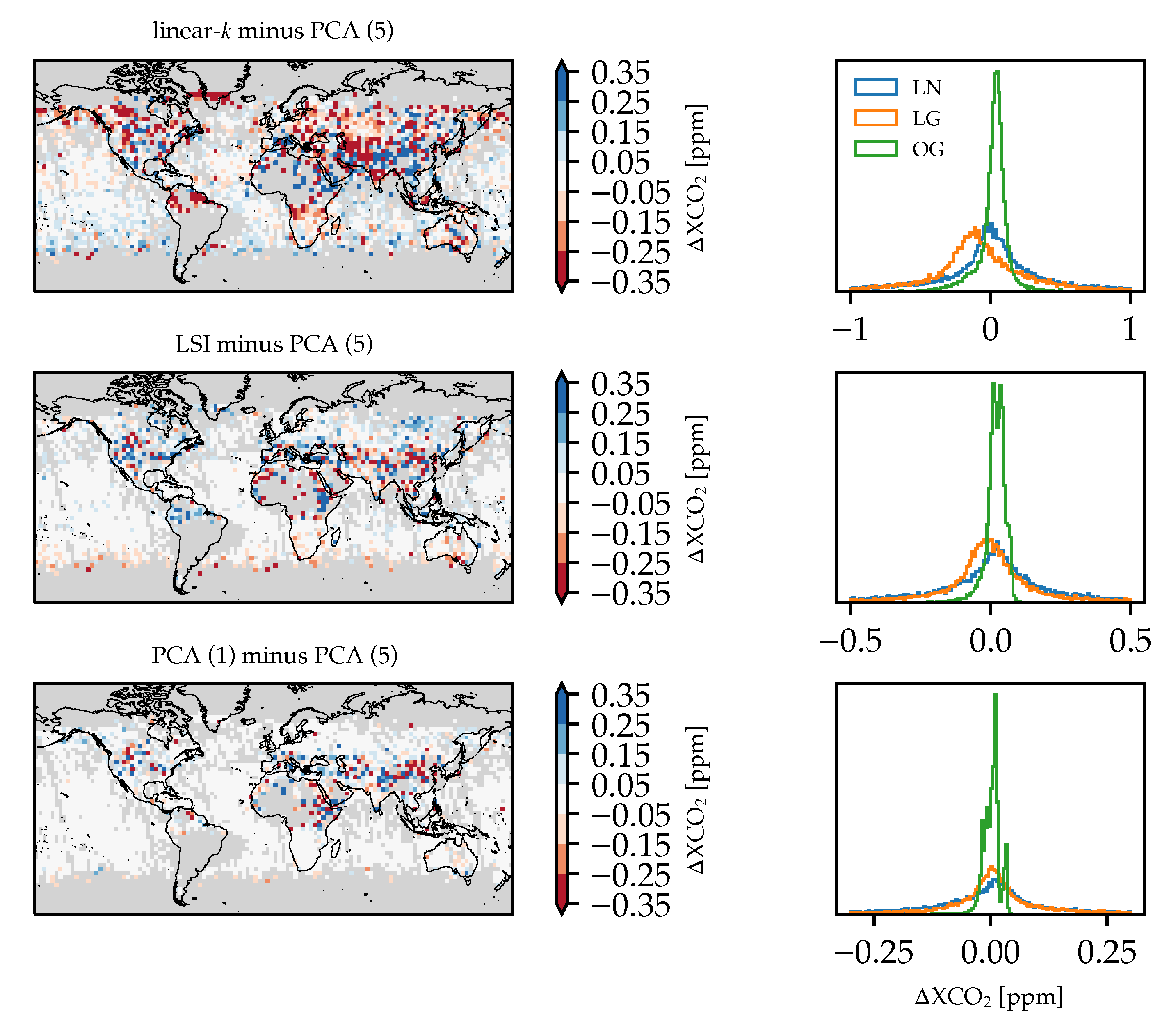
Figure 8 and Table 4 contain the main result of our study. We show that after representative post-retrieval filtering and parametric bias correction, the overall XCO${}_2$ bias between the various fast RT methods is generally below 0.05 ppm with an overall scatter of $\tilde{\sigma }<$ 0.70 ppm. The corresponding inter-quartile ranges (IQRs) do not exceed 0.40 ppm, and the differences between IQRs and $\tilde{\sigma }$ are larger for land nadir and land glint modes. This mostly reflects the long-tailed aspect of the distributions seen in Figure 8 for land scenes. The parametric bias correction procedure has a notable effect when assessing the retrieved XCO${}_2$ against the truth proxy which is used for the bias correction itself. Its impact is largest on ocean glint scenes where it reduces the scatter by over 50%. Comparing this to the pair-wise differences between retrieval sets, we observe that the impact is less across all observation modes and all compared pairs. We thus conclude that the bias correction procedure is roughly equally effective for all four retrieval sets, and, on average, adjusts the raw XCO${}_2$ values in a similar way. This is also underlined by the bias correction coefficients in Table 3 which show little difference between the four sets.

Putting the numbers of Table 4 into context, we can refer to overall biases and scatter of some XCO${}_2$ product against a global truth proxy. O’Dell et al. [31] state biases and scatter for overpasses over ground-based stations, which range between $\mathsf{\Delta }=0.06$ ppm and $\sigma =0.83$ ppm (ocean glint) to $\mathsf{\Delta }=0.30$ ppm and $\sigma =1.04$ ppm (land nadir). The same statistics against a set of global models exhibit similar values for bias and scatter (not shown in O’Dell et al. [31]). Given those numbers, we can see that the differences ($\mathsf{\Delta }$) of bias-corrected XCO${}_2$ from retrievals using different fast RT methods are generally smaller than overall biases to the truth proxies, by almost an order of magnitude. The way in which the overall scatter between fast RT sets would enter the XCO${}_2$ scatter of a retrieval–model truth comparison is not straightforward, mostly because a small, manual modification of filter thresholds can change those statistics. Focusing on mean biases alone, we can therefore assume that the choice of fast RT method would not cause a significant change in how a final XCO${}_2$ product compares to truth proxies on a global level. This is implicitly already shown in Buchwitz et al. 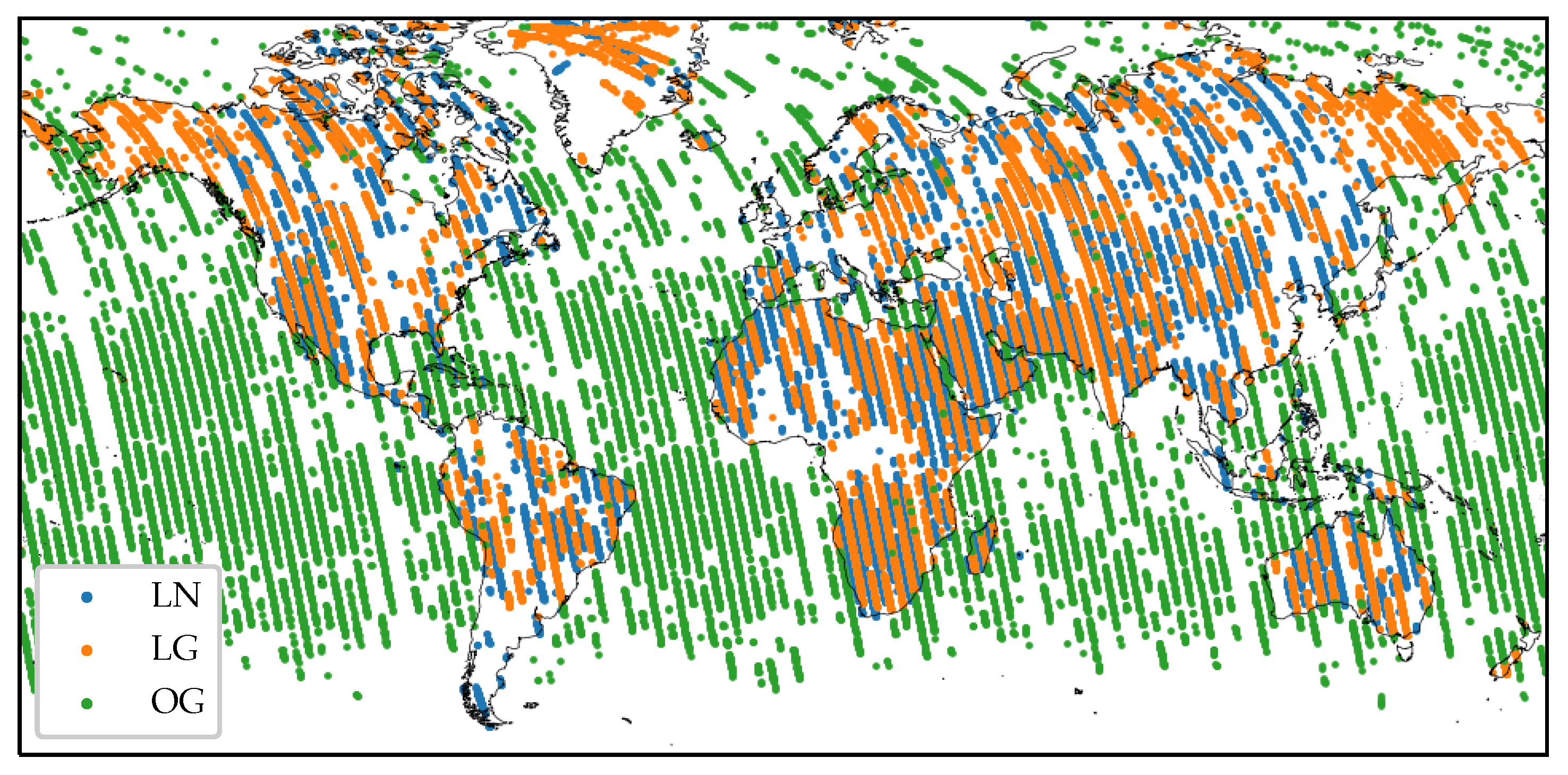[40], where several XCO${}_2$ and XCH${}_4$ retrieval sets were evaluated in a systematic way. However, the following caveats of our study have to be considered. We only observed a small set of OCO-2 scenes, which after coarse filtering leave the Sahara desert and South America regions mostly empty (see Figure 8). Those regions are known to be particularly difficult for XCO${}_2$ retrievals, as a result of either high aerosol loading due to mineral dust, or the presence of many small clouds that create biases via 3-D scattering effects [62]. As a result of our limited scene selection we are also biased towards clearer scenes in terms of aerosols, however it does not strictly follow that we can consider our obtained differences between fast RT methods as a lower bound.

The four retrieval sets across three different fast RT methods group somewhat distinctly into LSI and PCA on one side, and linear-k on the other side. As we have discussed in detail in Section 2.2, this grouping is expected due to the way these fast RT methods are designed on a fundamental level. The biggest discrepancy is related to Jacobians which have strong multiple-scattering contributions, such as any aerosol Jacobians. As the forward model is non-linear, even slight modifications to Jacobians can lead to different results for both the final XCO${}_2$ and the remaining portion of the state vector. We therefore employed a filtering and bias correction method for each individual retrieval set to systematically correct the raw XCO${}_2$ values in a manner that resembles the procedure done in most publicly available XCO${}_2$ data sets. Table 4 shows that the bias correction procedure reduces the inter-set spread, which was low to begin with ($\mathsf{\Delta }<0.1$ ppm). Looking at the values of the parametric bias correction coefficients in Table 3, we observe that values across a certain parameter range for a certain observation mode are comparable between the fast RT methods. The linear-k set behaves very similarly for land nadir observations and the $\delta {\nabla }_{{\mathrm{CO}}_2}$ parameter. For land glint observations, we see more discrepancies for both the $\delta {\nabla }_{{\mathrm{CO}}_2}$ and the $\mathsf{\Delta }{p}_{\mathrm{surf}}$ parameters. Finally, for ocean glint observations, the discrepancies pertain to the albedo ratio (${\rho }_1/{\rho }_2$) parameter only. These observations are also consistent with the notion that linear-k has a different sensitivity to aerosols—the retrieved CO${}_2$ profile is linked to the retrieved aerosol profiles through interference errors [35].

When we compare the bias-corrected XCO${}_2$ values against the individually sampled model medians (see Table 5), we observe that the linear-k set exhibits the most favourable statistics across all observation modes, despite comparable and sometimes larger numbers of quality-filtered scenes (see Table 2). When looking at the robust standard deviations as a measure of scatter, the linear-k set of retrievals shows between 0.02 ppm (land nadir) and 0.05 ppm (land glint) lower values. While the differences of scatter values themselves are statistically significant at $N\sim$ 20,000, we do not consider this as evidence of superior performance of linear-k over the other methods. A more thorough and automated process involving scene filtering and bias correction would be required to make an unbiased assessment when the differences are less than a tenth of a ppm. The results, however, suggest that the linear-k retrievals respond slightly more favorably to the filtering and bias correction process in our particular example. Despite that radiance residuals for PCA (1) can be twice as large as those of PCA (5) [33], those differences do not impact the overall comparison against the truth proxy. This particular observation suggests that one principal component is sufficient for OCO-2 XCO${}_2$ retrievals using the PCA-based method.

Bulk statistics, as stated in Table 4 and Table 5, of course, do not capture the entire characteristics of a pair-wise comparison of two XCO${}_2$ retrieval sets. Figure 8 show several regions in which significant differences occur. The overall most similar two sets of retrievals are the two runs using the PCA-based method. Only 124 out of 3049 grid cells (at $3^{\circ }\times 3^{\circ }$ aggregation), or roughly 4.1%, exhibit a difference larger than 0.3 ppm. Interestingly, bias correction does not change that number much (123 out of 3049 without parametric bias correction). This itself is somewhat remarkable as the radiance residuals are significantly dependent on the number of principal components used in the radiance reconstruction process (see Somkuti et al. 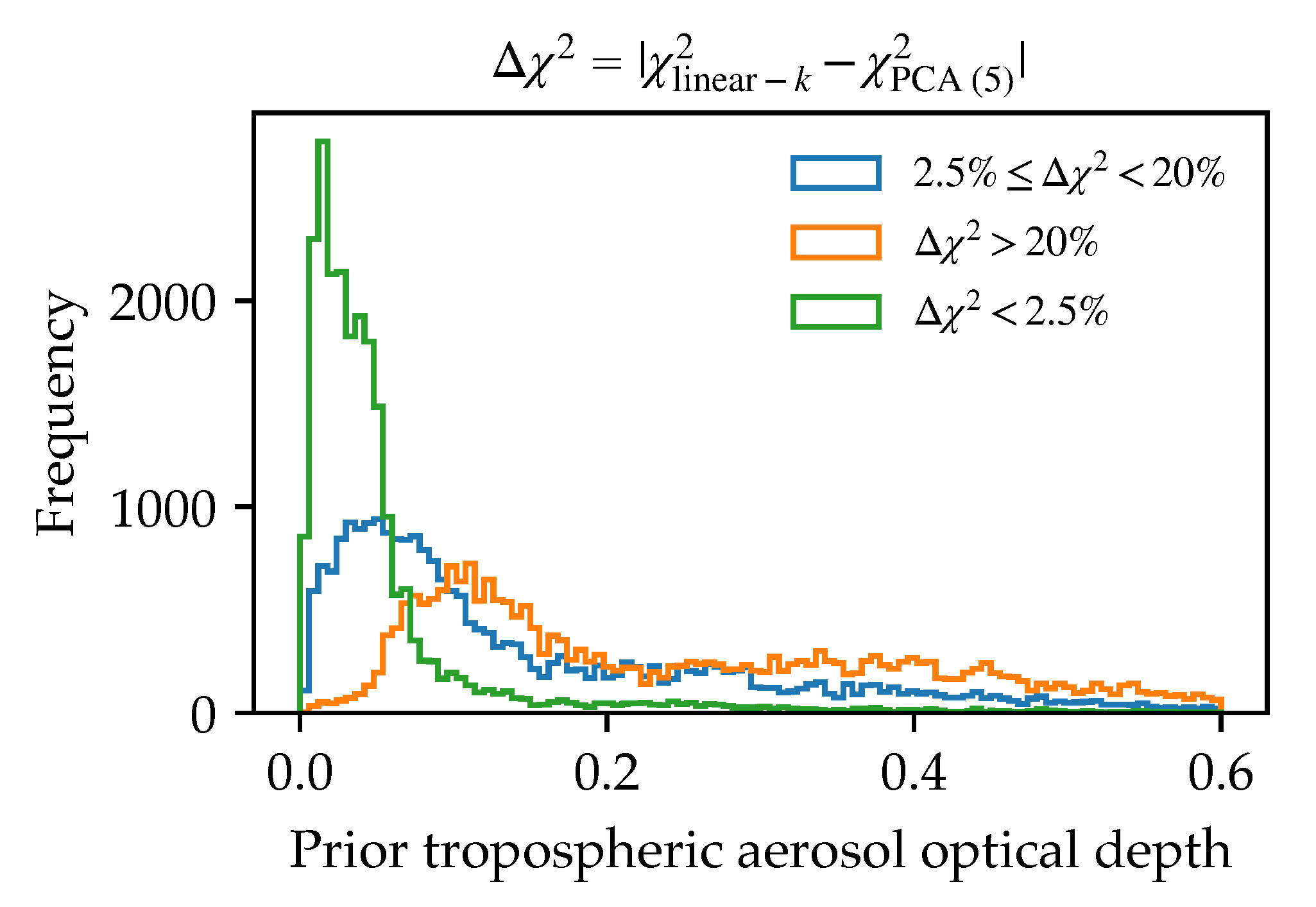[33]). When comparing the LSI set against the PCA (5) set, we observe more regional differences and the number of grid cells with differences larger than 0.3 ppm is 5.7% (171 out of 3020) after bias correction. Finally, comparing linear-k against PCA (5) shows 14.7% of $3^{\circ }\times 3^{\circ }$ grid cells (426 out of 2905) being more than 0.3 ppm apart (21.4% before bias correction). The different behavior in the comparisons linear-k↔ PCA (5) and PCA (1) ↔ PCA (5) suggest that the radiance reconstruction of the various fast RT methods have a smaller impact than the reconstruction of the Jacobians.

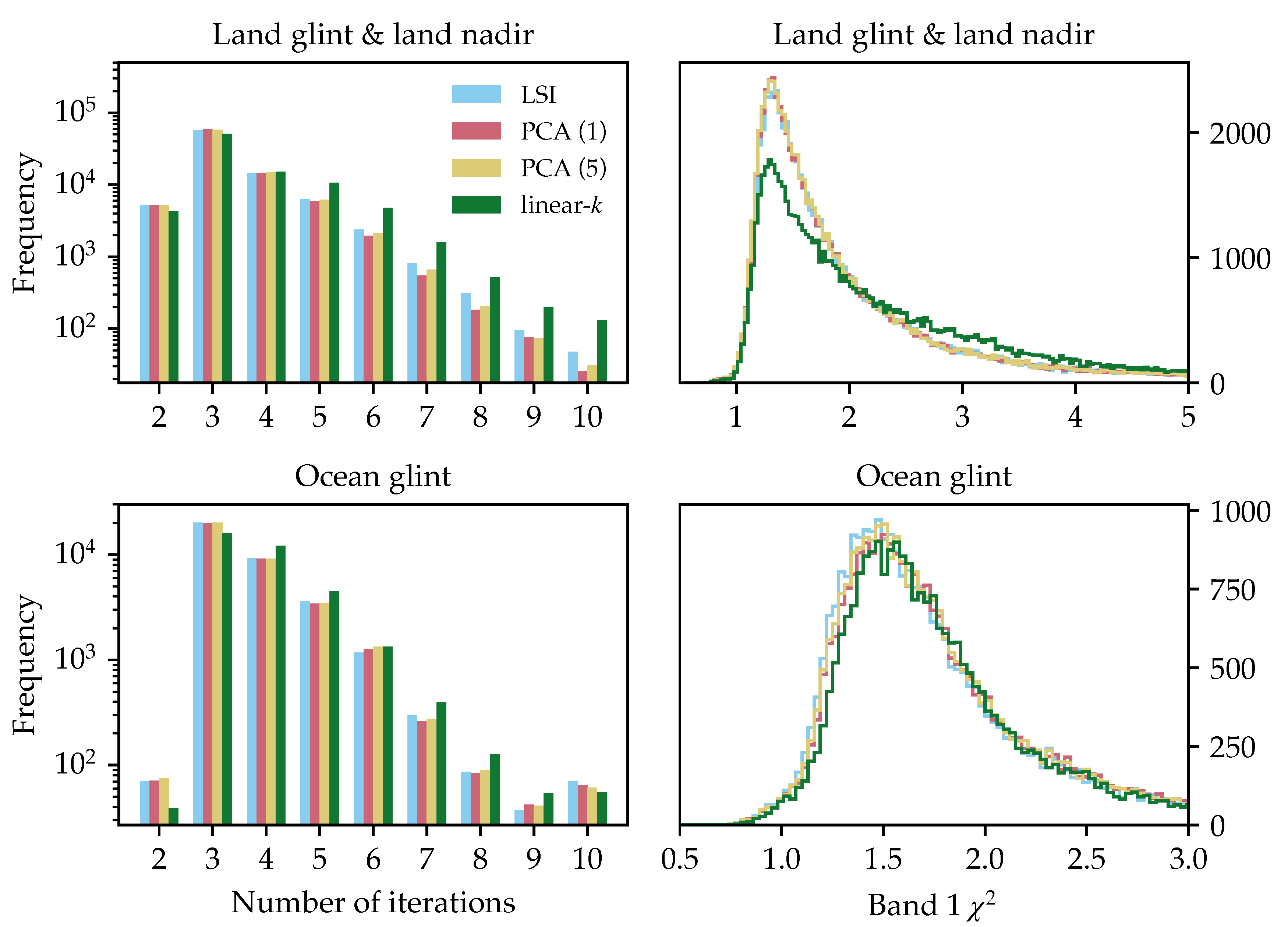
We want to stress the shortcomings of our study to also highlight where our results are applicable, compared to where they are not. The small subset processed in our study (see Section 2.3) does not allow for any small-scale analysis. This means our results cannot make any statements about discrepancies for e.g., city-scale XCO${}_2$ collections seen in OCO-3 [2]. Further, since we only use OCO-2 scenes which were already quality filtered, the selected scenes are overall biased towards lower aerosol loadings and are generally more well-behaved. This is evident in the number of iterations: more than 80% of all retrievals converge in four iterations or less. As already mentioned before, not all scenes necessarily fall into the “more clear” category, since we use the UoL algorithm setup, which, compared to the ACOS algorithm, sources different prior values for many state vector variables, most importantly aerosols. A look at Figure 8 reveals that regional differences can surpass ∼0.3 ppm, even for the comparison between PCA (1) and PCA (5), which would likely cause differences in applications such as surface carbon flux inversions [15]. Including a more extensive set, i.e., a longer time series, of OCO-2 scenes might change the pattern of regional differences as well as fill in areas which have no scenes at all in Figure 8. Moreover, the choice of fast RT method could also result in a changed seasonal cycle due to the impact of seasonally varying aerosol distributions. We believe the impact of the reconstruction accuracy of aerosol Jacobians to be significant, however that conclusion could hold only for the UoL algorithm. Other algorithms, such as RemoTeC, characterize and retrieve aerosols using a different approach (see e.g., Wu et al. [44]). Further, the aerosol sensitivity of OCO-2 is comparable to that of GOSAT and GOSAT-2, however not for instruments like CO2M as its spectral resolution is lower. In upcoming work, one could aim to disentangle the impact of weighting functions from the radiance reconstruction using a hybrid fast RT scheme: radiances could be reconstructed using one fast RT method, and Jacobians would be calculated using another method.

5. Conclusions

In this study, we implemented three contemporary fast radiative transfer (fast RT) methods into the UoL XCO${}_2$ retrieval algorithm. This allowed us to explore the impact of the choice of fast RT method with all other components of the retrieval algorithm being the same. We ran four sets of retrievals (with two different settings for the PCA-based method) and performed post-retrieval filtering as well as parametric bias correction to ensure that each set of retrievals is individually treated as they would in any XCO${}_2$ data set processing. The bulk differences in XCO${}_2$ between the four sets show just a small overall bias $\mathsf{\Delta }<0.1$ ppm, and the difference scatter being between $\tilde{\sigma }<0.65$ ppm ($\tilde{\sigma }$ being a robust standard deviation) for land nadir, and $\tilde{\sigma }<0.08$ ppm for ocean glint. Regional differences, however, can exceed 0.3 ppm (after bias correction) for 4% of the data points and can thus be considered significant biases. We find that land nadir observation modes exhibit the largest differences, and ocean glint scenes the lowest. In the comparison against CO${}_2$ models, which were also utilized as truth proxies for the parametric bias correction, linear-k shows the best performance, although the differences are too small to make a more general recommendation in the context of OCO-2 retrievals. Further studies, especially on small- and city-scale aggregates, need to be undertaken to understand the full impact of fast RT methods on XCO${}_2$ retrievals in the shortwave-infrared wavelength region. For example, the estimation of point-source emission rates, which relies on the determination of XCO${}_2$ (or XCH${}_4$) enhancements [9,63,64], can be affected by biases amongst other sources of uncertainty, such as wind direction and wind speed. Given the similarity of results between the PCA (1), PCA(5) and LSI sets of retrievals, we believe the reconstruction accuracy of atmospheric weighting functions related to aerosols to be a major driver of the observed discrepancies between linear-k and the other sets. Finally, the data quality filtering and bias correction approaches need to be formulated using a more autonomous and reliable technique to reduce the impact of manually chosen parameters and thresholds.