Article

Climate Sensitivity and Feedback of a New Coupled Model (K-ACE) to Idealized CO2 Forcing

1
Innovative Meteorological Research Department, National Institute of Meteorological Sciences, Seogwipo, Jeju 63568, Korea
2
Operational Systems Development, National Institute of Meteorological Sciences, Seogwipo, Jeju 63568, Korea
3
Numerical Model Development Division, Numerical Modelling Center, Korea Meteorological Administration, Seoul 07062, Korea
4
Met Office Hadley Centre, Exeter EX1 3PB, UK
*
Author to whom correspondence should be addressed.
Atmosphere 2020, 11(11), 1218; https://doi.org/10.3390/atmos11111218
Submission received: 4 September 2020 / Revised: 30 October 2020 / Accepted: 10 November 2020 / Published: 12 November 2020
(This article belongs to the Section Climatology)

Abstract

:
Climate sensitivity and feedback processes are important for understanding Earth’s system response to increased CO2 concentration in the atmosphere. Many modelling groups that contribute to Coupled Model Intercomparison Project phase 6 (CMIP6) have reported a larger equilibrium climate sensitivity (ECS) with their models compared to CMIP5 models. This consistent result is also found in the Korea Meteorological Administration Advanced Community Earth System model (K-ACE). Idealized climate simulation is conducted as an entry card for CMIP6 to understand Earth’s system response in new coupled models and compared to CMIP5 models. The ECS in the K-ACE is 4.83 K, which is higher than the range (2.1–4.7 K) of CMIP5 models in sensitivity to CO2 change and higher bound (1.8–5.6 K) of CMIP6 models. The radiative feedback consists of clear-sky and cloud radiative feedback. Clear-sky feedback of K-ACE is similar to CMIP5 models whereas cloud feedback of K-ACE is more positive. The result is attributable for strong positive shortwave cloud radiative effect (CRE) feedback associated with reduced low-level cloud cover at mid latitude in both hemispheres. Despite the cancellations in strong negative long wave CRE feedback with the changes in high-level clouds in the tropics, shortwave CRE has a dominant effect in net CRE. Detailed understanding of cloud feedback and cloud properties needs further study.

1. Introduction

Climate sensitivity (ECS; equilibrium climate sensitivity) is typically defined as the average global temperature rise following a doubling of CO2 concentration in the atmosphere compared to pre-industrial levels. It results from a variety of feedback processes (e.g., Planck feedback, water vapor feedback, cloud feedback, and radiative feedback) within the global climate [1,2,3,4,5,6]. Thus, it is essential to identify and understand the specificity of climate system warming in response to increased CO2 levels in climate projection.
The ECS is important for effective carbon reduction polices to achieve a specific warming target [7]. For example, pre-industrial CO2 is approximately 260 parts per million (ppm), and hence, doubling would be approximately 520 ppm. Current levels of atmospheric CO2 have exceeded 410 ppm, with the 520-ppm threshold expected to be surpassed in the next 50–100 years based on predicted future greenhouse gas emissions. Additionally, Matthews et al. [8] found that global warming depends mainly on the total cumulative anthropogenic emission of CO2 and the details of the emission pathways are of secondary importance to warming. The larger ECS indicates that a smaller amount of carbon can still be emitted to limit the warming levels suggested by the Paris Treaty. Therefore, when more specificity regarding the dynamics of climate sensitivity are understood, it would be useful to estimate the amount of CO2 we can emit and remain below 2 °C of warming [9,10,11,12].
ECS is also a widely used metric to illustrate the temperature increase that would eventually occur when the climate system fully adjusts to a sustained doubling of CO2 [13,14,15]. It is challenging to determine its value with observations or models [16,17]. Currently, the majority of CMIP5 [18] model estimates have an ECS, in the range of 2.1–4.7 K [19]. Several studies of individual CMIP6 models [20,21,22,23,24] report that higher values of ECS are largely due to stronger cloud feedbacks. Recently, this has been reported as a common feature in CMIP6 models [25,26,27], and the relationship between surface warming trend and climate sensitivity has also been reported for a transient climate response (TCR) [27,28,29,30]. The National Institute of Meteorological Sciences/Korea Meteorological Administration (NIMS/KMA) has participated for CMIP5 experiments under collaboration with UK-Met Office (UKMO) using HadGEM2-AO [31]. However, only HadGEM2-ES, which has a family configuration, was used in idealized climate change experiments (abrupt 4 × CO2 experiment) in CMIP5, and this model shows 4.6 K of ECS [32]. It has increased to 4.83 K of ECS in the new coupled model (K-ACE) and has a higher sensitivity compared to CMIP5 range. Considering this, a higher ECS has important consequences, such as increased warming in the 21st century emission scenario, increased risk of feedbacks, and an impact on allowable carbon budgets for a given target. However, the complexity of the model development process makes this impossible. Several previous studies [22,33] have attempted to investigate the reason for this based on the development in a systematic and continuous approach. From this perspective, this is a first attempt that assesses climate sensitivity and their feedbacks using K-ACE. This study attempts to evaluate the climate sensitivity and quantifies the sensitivity of radiation change to CO2 forcing in K-ACE, which is the first participant model for CMIP6. Section 2 presents a brief introduction of K-ACE and its relevant experiments and methods. Section 3 describes global climate sensitivity and feedback with a primary focus on radiative feedback. Lastly, Section 4 presents a summary and discussion.

2. Model Experiment and Methodology

The K-ACE is a coupled climate model (Atmosphere–Ocean–sea Ice–Land; AOIL), and detailed component models (the number of physical and biogeochemical processes included) with coupling approaches are described in Lee et al. [34]. Hence, limited details are given here. The Unified Model (UM) in the Global Atmosphere 7.1, the latest configuration [35], is the atmospheric component of the K-ACE. A new dynamics scheme, the Even Newer Dynamics for General atmospheric modeling of the environment (ENDGame) [36], is implemented for faster and more efficient model integrations. Atmospheric radiative transfer is calculated by Suite of Community Radiative Transfer codes based on Edwards and Slingo (SOCRATES) [37], and tropospheric aerosols are calculated using the GLObal Model of Aerosol Processes (GLOMAP) [38,39] that considers the number concentration, size distribution, composition, and optical properties of aerosols based on the aerosol microphysics and chemistry. The ocean component is the Modular Ocean Model of GFDL (MOM) [40] and the Sea Ice model of Los Alamos (CICE) [41] is used for the sea-ice component. These components are coupled using the OASIS3–MCT coupler [42,43]. The horizontal resolution is N96 (~135 km) with a regular latitude–longitude grid in the atmosphere and a tri-polar grid in the ocean. Additionally, the vertical resolution is 85 levels (L85) in the atmosphere and 50 levels (L50) in the ocean. There are increased vertical levels in the atmosphere compared to a previous version of UM (38 levels). Moreover, there are many changes to the atmospheric physics; however, the new mixed-phase cloud scheme (PC2) is most significant [44,45], which uses three prognostic variables for water mixing ratio (water vapor, liquid, and ice) and cloud fraction (liquid, ice, and mixed-phase). Compared to the previous cloud scheme [46], the PC2 cloud scheme has a direct physical link between condensate, cloud fraction, and the physical processes that lead to their production. Additionally, it does not contain a separate, diagnostic large–scale cloud scheme [44]. Thus, the radiative effects of cloud related to convection are represented in the large-scale fields. Wilson et al. [45] reports that this approach offers the advantage of a more physically realistic cloud process. Overall, the PC2 cloud scheme leads that the ice cloud fraction extends higher (decrease low-level cloud) and high cloud cover is increased in tropics and high latitudes [45].
The 23 members of CMIP5 models and 18 members of CMIP6 models are used in this study (available members from the Earth System Federation Grid (ESGF) nodes at the time of writing). In CMIP6, as in earlier CMIP phases, the pre-industrial control (hereafter referred to as the pi-Control) simulation is an attempt to produce a stable quasi-equilibrium for beginning state of CMIP abrupt 4 × CO2 experiment (hereafter referred to as the abrupt experiment). Additionally, this experiment is now included in the standard Diagnostic, Evaluation, and Characterization of Klima (DECK) experiments, which is a requirement for participation in the CMIP6 [47]. Modeling groups routinely calculate climate sensitivity for each new model version. Considering these points, the ECS for K-ACE is calculated from the CMIP abrupt 4 × CO2 experiment (hereafter referred to as the abrupt experiment), and the CO2 concentration (1136.8 ppm) is abruptly quadrupled from the global annual mean from the year 1850 (284.2 ppm). A useful method to calculate ECS via abrupt experiment is proposed by Gregory et al. [48], which is estimated by comparing the response of the top of atmosphere (TOA) radiative flux and surface air temperature (ECS value as one-half of the x-intercept and the total climate feedback parameter as the slope of the regression). This method has been widely used to provide ECS of climate models [25,26,27,30]. Shortwave (SW) and Longwave (LW) feedback parameters are calculated using a similar concept; however, the TOA radiative fluxes are applied anomalies instead of total value.

3. Results

3.1. Climate Sensitivity to Idealized CO2 Change

Figure 1 shows the global annual mean surface air temperature changes from the abrupt experiments. The simulated period is 150 years, of which we regard the first 20 years as the transient part and the remaining 130 years as the equilibrium state. During the simulated period, the surface temperature does not stabilize. Compared to the 23 models from CMIP5, the temperature changes in K-ACE warms more in response to increased CO2 (5–95% confidence levels). This is similar result with other CMIP6 models (HadGEM3-GC3.1-LL and UKESM1 [22], CNRM-CM6 [20], CESM2 [23], EC-Earth [21], and E3SMv1 [24]).
Figure 2a shows the global annual mean change in net TOA radiative flux as a function of global mean surface temperature change. This regression has been expressed by Gregory et al. [48] for a simple linear relationship between radiative forcing and climate response. This approach considers that global surface temperature is unchanged. Therefore, climate feedback processes have an impact on the TOA radiation balance, which is included in our forcing estimate. Based on the Gregory-style regression, net climate feedback λ (Figure 2a), the slope of fitting line, is approximately −0.69 Wm−2 K−1, and ECS of K-ACE is 4.83 K. Figure 2b shows the ECS of CMIP5 and CMIP6 models. It is observed that the ECS of CMIP6 with values spanning 1.8–5.6 K is larger than the range of CMIP5 (2.1–4.7 K). Recently, many studies reported that the ECS from several CMIP6 models has increased substantially [20,21,22,23,24]. The ECS of K-ACE is higher than that of CMIP5 and near high bound of CMIP6 models (Figure 2b).
Previous studies report that a wide range of ECS values produced by global climate models and its uncertainty are mainly caused by radiative feedbacks [17,20,22,49]. To understand the difference in the climate sensitivity of K-ACE regarding the radiative feedback compared to CMIP5 and CMIP6 models, the global mean radiative feedback contribution of ECS are divided into feedbacks at clear-sky and cloud sky. In Figure 3, radiative feedback components are calculated as the slope of the linear fit of radiative flux change against temperature change for 150 years [48]. Hereafter, net radiative feedback, clear-sky feedback, and cloud radiative effect feedback are represented by λNET, λCS, and λCRE, respectively. SW and LW components of clear-sky feedback and cloud radiative effect are indicated by λSWCS, λLWCS, λSWCRE, and λLWCRE, respectively. The CRE is defined as the difference between all-sky and clear-sky net radiative fluxes.
Taken individually, cloudy components of the net feedback are significant outliers from the CMIP5 average and clear-sky components mostly fall within the range of CMIP5 and CMIP6 models. Under clear sky, the λSWCS and λLWCS of K-ACE are 0.61 Wm−2 K−1 and −1.82 Wm−2 K−1, respectively. The combination of λSWCS and λLWCS results in negative λCS of K-ACE showing similar magnitude with CMIP5 models. The cloud components of K-ACE are strong positive λSWCRE with 0.97 Wm−2 K−1 and negative λLWCRE with −0.46 Wm−2 K−1, and both λSWCRE and λLWCRE are extreme in the range of CMIP5 model spread. Senior et al. [32] reports that λSWCRE and λLWCRE of HadGEM3-GC2 tend toward the higher and lower ends of the range of CMIP5 models. K-ACE also shows the similar results. Similarly, the range of the λSWCRE and λLWCRE for CMIP6 models extend in a positive and negative direction, respectively, compared to CMIP5 models. Overall, positive λCRE in K-ACE, even with cancellation by negative λCS, contribute to high bound of λNET (small absolute value), leading to high values of ECS. Andrews et al. [22] and Golaz et al. [24] suggest that an unusual combination of forcing and feedback leads to a higher ECS. This relationship between λNET and ECS is also represented. Additionally, the spread of λCRE in inter-model differences is larger than that of λCS and model spread of λNET is influenced by a wide spread of λCRE. Considering this, λCRE is the key contributor of uncertainty (Figure 3), which is comparable with many previous studies [7,17,20,22,32,49,50,51,52].
Many studies have focused on the analysis of radiative feedback in clear and cloudy sky conditions [7,32,53,54] and on the differences in the SW cloud feedback [49,55,56,57]. Further, Ceppi et al. [6] reports that the contributions to λSWCRE and λLWCRE are far from being spatially homogeneous which is influenced by cloud distribution. Therefore, global patterns of corresponding feedback components are also investigated in this study for understanding the effect of CRE feedback to higher ECS.
The difference in λNET between the CMIP5 ensemble and K-ACE is significant in spatial distribution (Figure 4). Unlike an El Niño-like pattern in the mean field of CMIP5 models, the λNET of K-ACE occurs positively over the whole Pacific region and strong negative feedback occurs in the maritime continent (Figure 4a,b). These areas are strongly related to where cloud processes are important, such as in the Madden–Julian oscillation and monsoon system, and may be attributed to the improvements in the cloud process simulations due to the implementation of new cloud microphysics scheme [32]. Over the Tibet area (high altitude), a stronger positive feedback compared to CMIP5, is due to the decrease in albedo. However, the λNET of CMIP6 ensemble shows similar distribution with CMIP5 except for a positive value in the high northern latitude (Figure 4c). In general, the difference between the K-ACE and CMIP5/CMIP6 ensemble is larger over the ocean than over land.

3.2. Decomposition of Radiative Feedabck

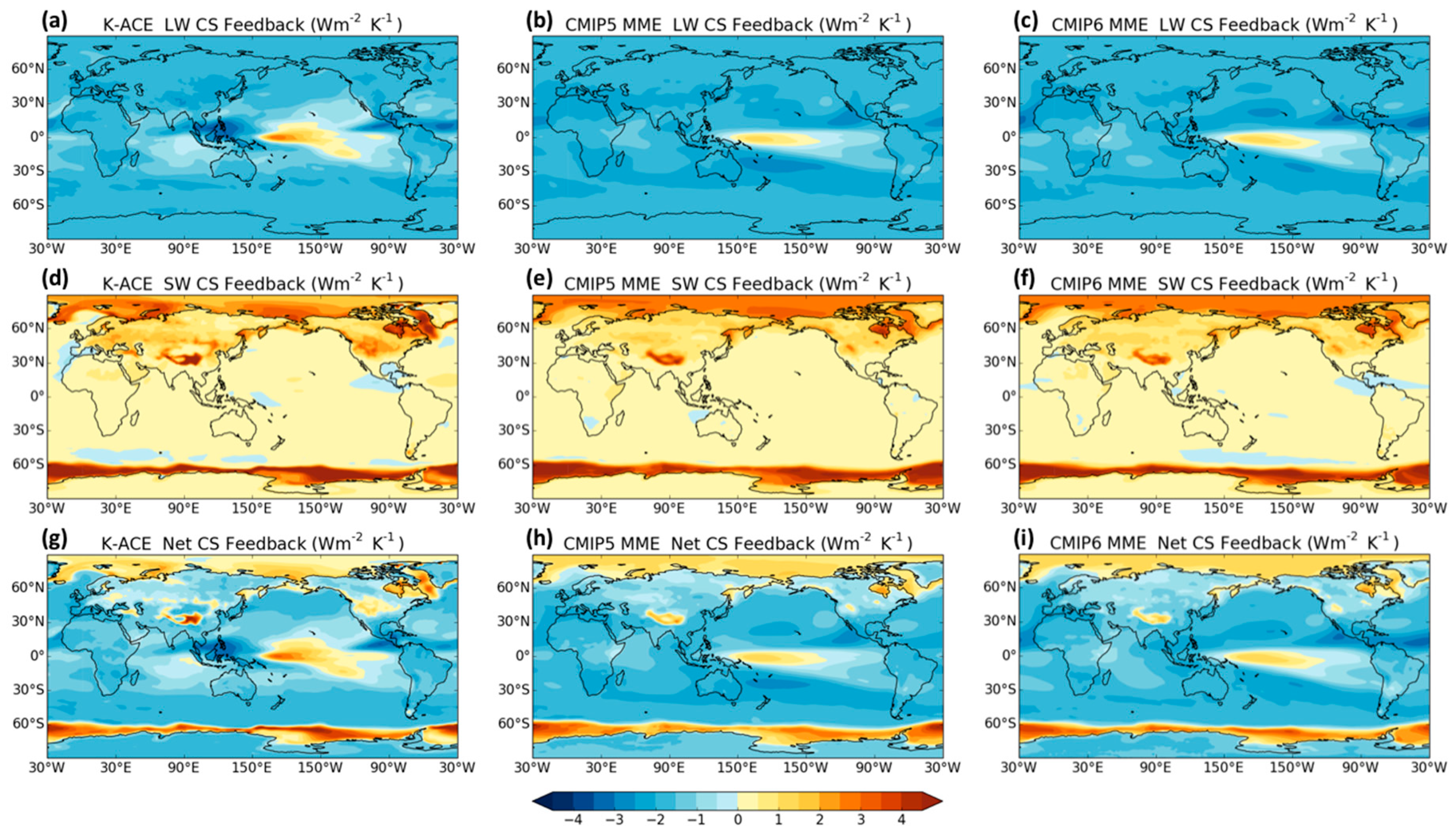
3.2.1. Clear-Sky Feedback
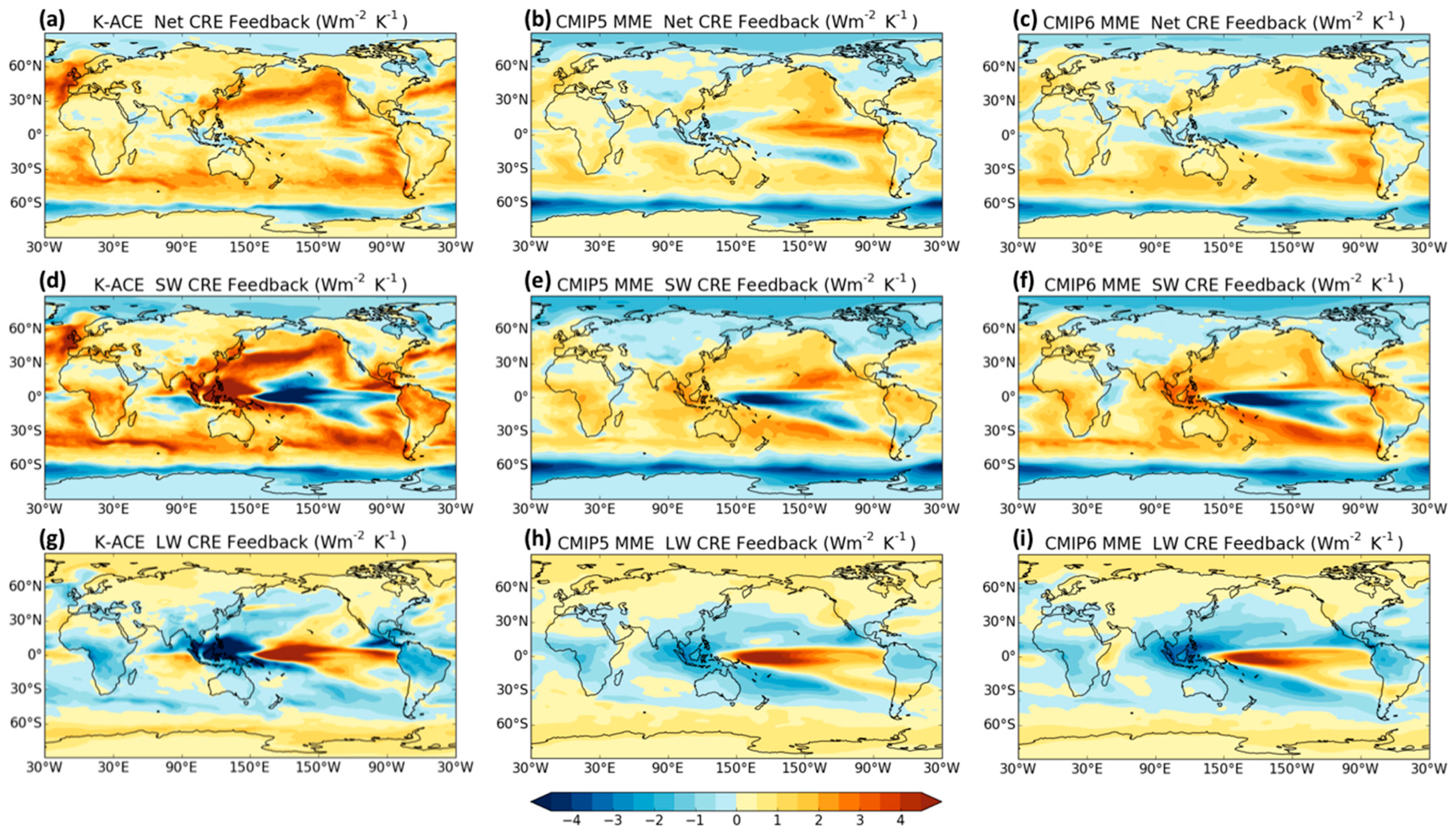
In Figure 3, λLWCS, λSWCS, and λCS of the K-ACE are within the range of CMIP5 models. The λLWCS is the most important negative feedback (Figure 5a–c) contributing to negative λCS to maintain the stability of the climate system after the appearance of a strong external perturbation [7]. Those clear-sky components of K-ACE show similar spatial patterns to the CMIP5 and CMIP6 results whereas the magnitude in λSWCS of K-ACE is slightly weaker than of those models, which is due to the Arctic region (Figure 5d–f). There is large positive λCS of K-ACE in high latitude areas and high-altitude areas (Figure 5g–i), reflecting the warming effect of sea-ice melting [7]. These have been consistent with reduced clear-sky albedo due to a loss of sea-ice and snow cover with increased global temperature [34].

3.2.2. CRE Feedback

CRE feedback is positive in CMIP5, and CRE feedbacks play an important role in the higher sensitivity in GCM [54]. Additionally, CRE feedback is the main contributor to the uncertainty in climate sensitivity [53] and exhibits the largest amount of inter-model spread, originating primarily form the SW effect. The λCRE of CMIP5 and CMIP6 ensemble depends on strong positive λSWCRE with the compensation of negative λLWCRE across the tropical Pacific (Figure 6). Moreover, opposite tendencies of λSWCRE and λLWCRE occur horse-shoe patterns over subtropical Pacific and maritime continent, as clouds reflects solar radiation into space and block LW radiation from the surface. This is related to the increased sea surface temperature in the East Pacific as the El Niño-like response.
The spatial distribution of CMIP5 and CMIP6 CRE feedback and K-ACE is clearly different (Figure 6a–c). The opposite tendencies in λSWCRE and λLWCRE patterns are also found in K-ACE over the tropical Pacific. However, strongly positive λSWCRE and negative λLWCRE occurred in K-ACE over the tropical Western Pacific and Philippines region compared to the CMIP5 and CMIP6 ensemble means (Figure 6d–i). K-ACE also shows positive λSWCRE in the ocean and at mid-latitudes (approximately 30° N and S), enhancing positive λCRE. This is a different pattern of El Niño-like patterns represented in the CMIP5 and CMIP6 ensemble (Figure 6b,c). However, as mentioned in previous studies [7,32], the spatial pattern of λCRE is dominated by positive a λSWCRE, which is investigated in K-ACE (Figure 6a,d).

3.3. Cloud Properties Related to CRE Feedback

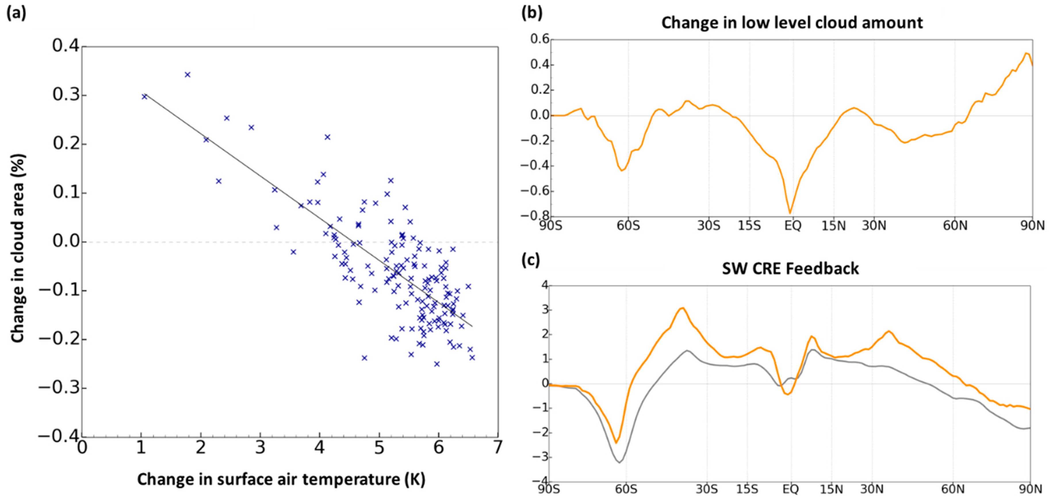
3.3.1. Low-Level Cloud Amount

Andrews et al. [22] reported that a new mixed-phase cloud scheme effects cloud feedback. Considering this, the relationship between simulated cloud properties based on the cloud scheme and λCRE are investigated in this study. This approach may provide a new hint further understanding of the model spread of λSWCRE and λLWCRE. In previous study, Senior et al. [32] reports that a new prognostic cloud fraction and condensation scheme [44,45] may contribute to a strong cloud radiative response. This new mixed-phase cloud scheme shows improved cloud formation (well-behaved in the very low and high cloud fraction) in the maritime continent as well as tropical and subtropical region [44,45] and has been implemented by UM in GA7.1. The family models of HadGEM3 include this physics scheme; K-ACE has also used this scheme.
As shown in Figure 7a, low-level cloud tends to decrease during warming, which in turn affects the positive λSWCRE compared to CMIP5 models (Figure 3; Figure 6a). Hence, the characteristic of the K-ACE cloud scheme (less low-level cloud) makes λSWCRE stronger compared to CMIP5 models. This is similar to Chen et al. [7], where the λSWCRE change of CAMS-CSM (one of CMIP6 model) is explained by low-level cloud change. Based on the characteristics of cloud scheme, the amount of low-level ice cloud of K-ACE is reduced in the mid-latitudes, decreasing albedo contributions to surface warming [44,45]. This process causes a positive λSWCRE in the mid-latitude compared to CMIP5 models (Figure 7b,c). Figure 7b indicates low cloud feedback, and the zonal mean of low cloud feedback is calculated by the global distributions of the slope in Figure 7a. Additional evidence suggests that decreasing tropical low cloud (15° S–15° N; Figure 7b) with increasing temperature makes stronger λSWCRE compared to CMIP5 (Figure 7c; increasing temperature produces less low clouds, more incoming radiation, and increased warming) that are directly related to cloud formations in K-ACE. Increased higher anvil cloud (less low-level cloud) in the tropical Pacific [45] contributes to a stronger λSWCRE. In addition, λSWCRE increases in mid-latitude, which is consistent with Andrews et al. [22]. This difference of λSWCRE is at mid-latitudes due to mixed-phase cloud and their interactions [22]. Overall, less low cloud (stronger λSWCRE) from K-ACE implies a stronger response to CO2 and this makes higher ECS.

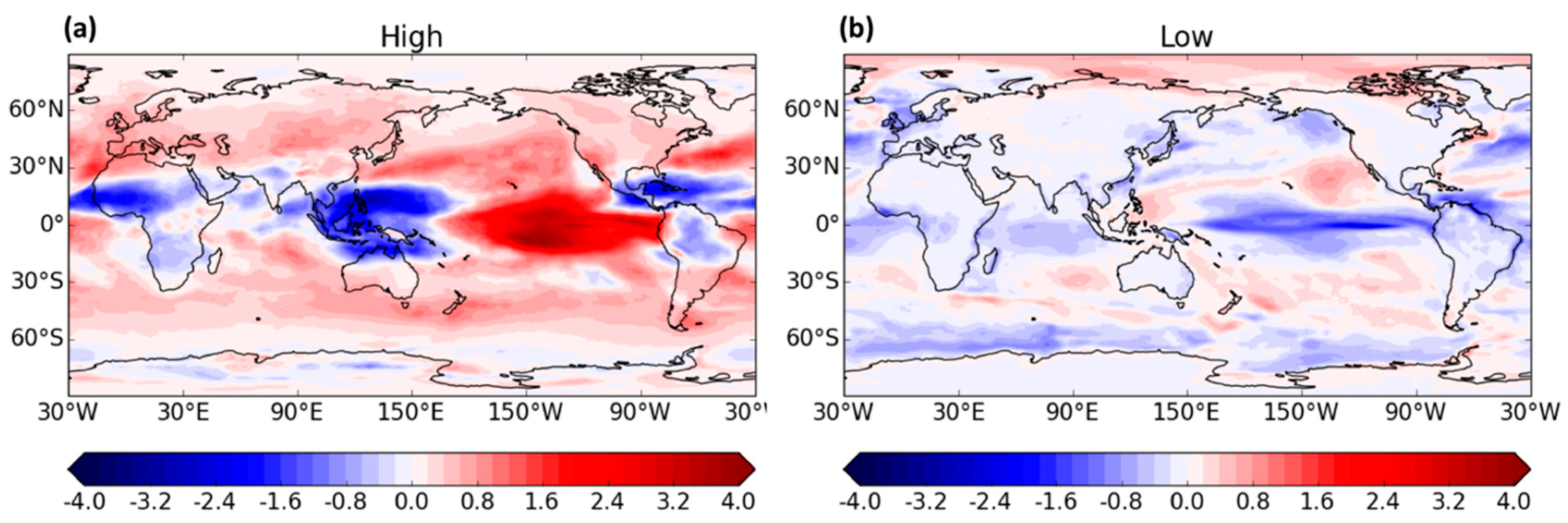
3.3.2. Higher Altitude Cloud

Figure 8a shows a global pattern of high cloud feedback (calculated by linear regression between change in cloud area (%) and surface air temperature (K); similar to the slope in Figure 7a). The red and blue shadings indicate increasing and decreasing cloud area with increasing temperature, respectively, and darker shading means a higher response of CO2. For high-level clouds, the cloud decreases over the maritime continent and increases over the tropical Pacific (Figure 8a). Moreover, high-level cloud increases over the subtropical areas. Based on the characteristics of cloud altitude in K-ACE, the mid-level cloud amount has effectively decreased due to the greater amount of high anvil cloud (increased high-level cloud due to the moistening in the upper tropical troposphere) [45]. Higher cloud tops are colder and emit less radiation to space. Therefore, an increase in the altitude of cloud top leads to warming by reducing outgoing LW radiation. This result is consistent with Andrews et al. [22] who demonstrated that a large high cloud response exists, which leads to a higher net cloud feedback. Additionally, the global pattern of λLWCRE (Figure 6c) and cloud feedback (Figure 8a) is spatially similar. Considering this, a higher cloud formation of K-ACE compared to CMIP5 models contribute to stronger λLWCRE, which could result in higher ECS.
Additionally, there is a cancellation of λSWCRE and λLWCRE in the tropical Pacific as expected for the increased amount of high-level cloud in this region (Figure 6a,c). Overall, λCRE is small in tropics (Figure 8b), which emphasizes that the amount changes of low-level cloud are important.

4. Conclusions

This study describes model characteristics for high climate sensitivity of K-ACE which has been developed by NIMS/KMA as part of participating in CMIP6. Abrupt experiments, as an entry card to CMIP6, are analyzed for climate sensitivity and feedback processes, and compared to 23 CMIP5 models and 18 CMIP6 models. Climate sensitivity is defined as the global temperature response to a doubling CO2 concentration in the atmosphere compared to pre-industrial levels. It is a basic metric of the climate research and essential for carbon reduction policies to achieve a specific warming target [7]. Recently, it is reported that the ECS in CMIP6 models has increased compared to CMIP5 and cloud feedback is considered the main cause [20,21,22]. Following this, we have analyzed the ECS and related feedbacks for K-ACE in a similar way and the results are summarized as follows.
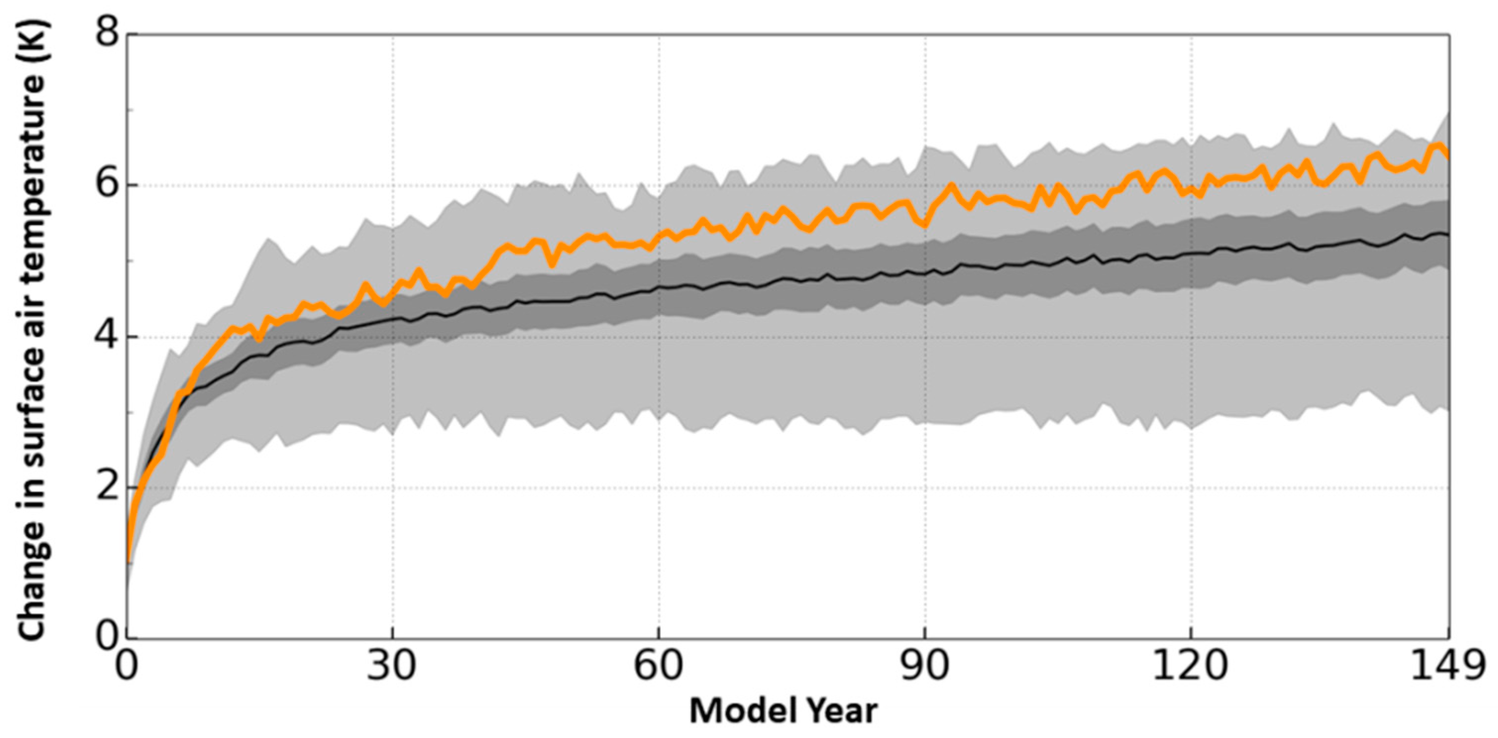
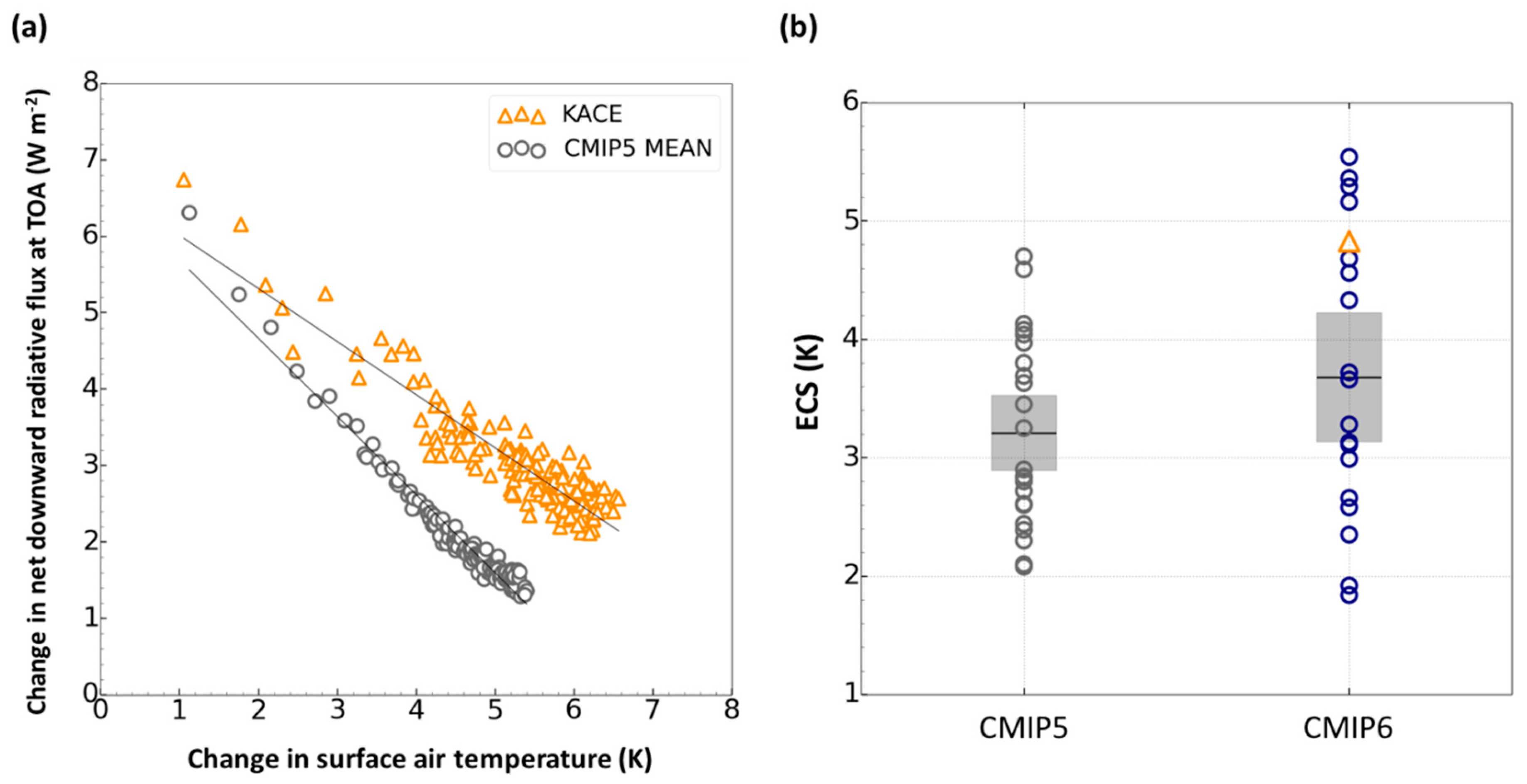
  • In the idealized CO2 experiment, temperature rising in K-ACE is larger than in the CMIP5 ensemble mean. The ECS of K-ACE calculated by Gregory et al. [48] is 4.83 K, substantially higher than the range of CMIP5 of 2.1–4.7 K and the higher bound of 1.8–5.6 K of CMIP6 models.
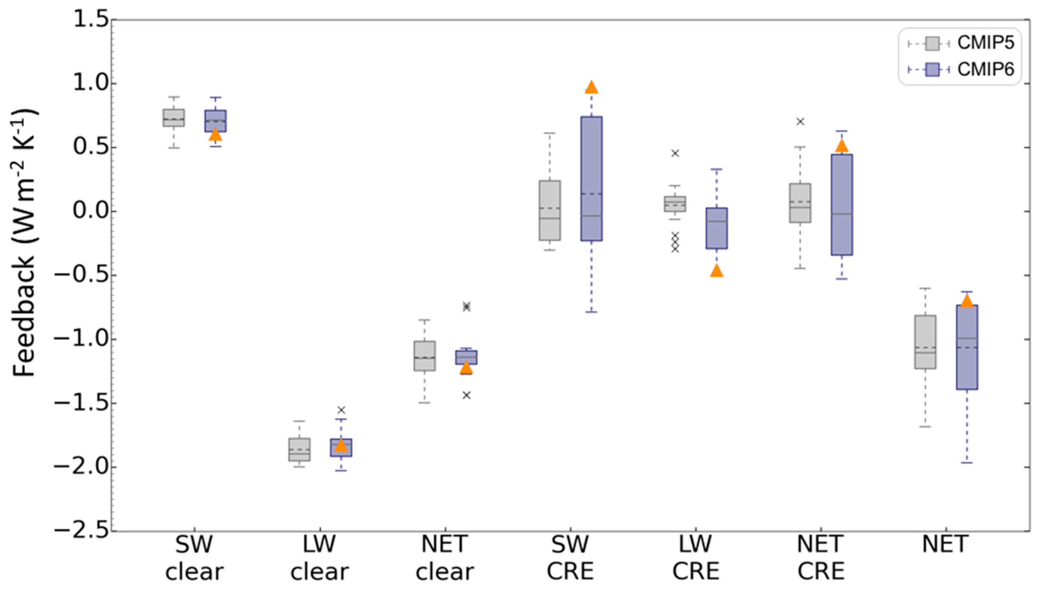
  • Radiative feedback is decomposed by clear-sky and cloud radiative feedback effects. Under clear skies, λSWCS and λLWCS are within the range of CMIP5 and CMIP6 models. Meanwhile, CRE feedback of K-ACE shows large amplitude. SW and LW components of CRE feedback (λSWCRE, λLWCRE) tend toward the higher and lower end of the range of CMIP5 and CMIP6 models.
  • Based on the cloud characteristics of K-ACE, less ice cloud in mid-latitudes (decreasing albedo, more surface warming) and less low-level cloud in the tropics (increasing temperature produces less low clouds, more incoming radiation, and increased warming) contribute to a stronger λSWCRE and higher ECS.
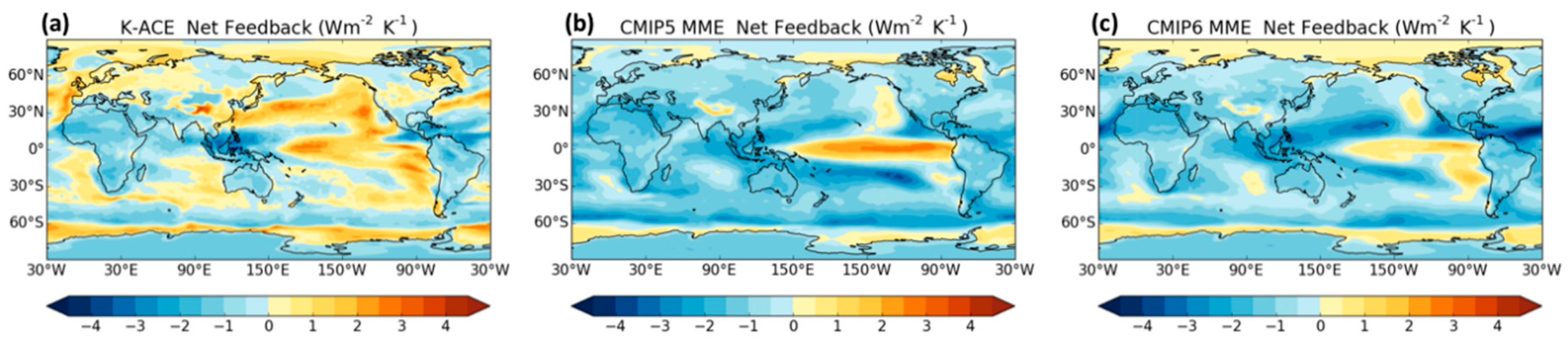
  • For high-level cloud, cloud characteristics of K-ACE (more high cloud due to the moistening in the upper tropical troposphere) contribute to less outgoing LW. In addition, the global pattern of λLWCRE (Figure 6d) and cloud feedback (Figure 8a) is spatially similar. This infers that higher cloud formation of K-ACE compared to CMIP5 models contributes to stronger λLWCRE, which could cause higher ECS.
The relationships between simulated cloud properties based on cloud scheme and λCRE are presented in this study. This approach provides some understanding of the cloud feedback based on cloud properties (amount and altitude). However, there are several limitations in this approach. The various climate models participated in CMIP6 have implemented different cloud schemes and CRE feedback is too complex to decompose into contributions from several cloud properties. Therefore, further work is necessary to understand the criteria for determining the spatial pattern of a cloud formulation related cloud scheme and the influence of these patterns on cloud properties at regional and global scales.

Author Contributions

Conceptualization, M.-A.S., H.M.S., K.-O.B. and Y.-H.B.; Formal analysis, M.-A.S.; Investigation, M.-A.S.; Methodology, M.-A.S. and H.M.S.; Project administration, Y.-H.B.; Resources, C.M.; Software, J.K.; Validation, M.-A.S.; Visualization, M.-A.S.; Writing—original draft, M.-A.S., H.M.S., K.-O.B. and Y.-J.L.; Writing—review & editing, M.-A.S., H.M.S. and K.-O.B. All authors have read and agreed to the published version of the manuscript.

Funding

This work was funded by the Korea Meteorological Administration Research and Development Program “Development and Assessment of IPCC AR6 Climate Change Scenarios” under Grant (KMA-2018-00321).

Conflicts of Interest

The authors declare no conflict of interest.

References

  1. Stocker, T.F.; Qin, D.; Plattner, G.K.; Tignor, M.; Allen, S.K.; Boschung, J.; Nauels, A.; Xia, Y.; Bex, V.; Midgley, P.M.; et al. Climate Change, 2013: The Physical Science Basis. Contribution of Working Group I to the Fifth Assessment Report of the Intergovernmental Panel on Climate Change; Technical Summary; Cambridge University Press: Cambridge, UK; New York, NY, USA, 2013; p. 1535. [Google Scholar]
  2. Held, I.M.; Soden, B.J. Water vapor feedback and global warming. Annu. Rev. Energy Environ. 2000, 25, 441–475. [Google Scholar] [CrossRef] [Green Version]
  3. Randall, D.A.; Wood, R.A.; Bony, S.; Colman, R.; Fichefet, T.; Fyfe, J.; Kattsov, V.; Pitman, A.; Shukla, J.; Srinivasan, J.; et al. Climate models and their evaluation. In Climate Change 2007: The Physical Science Basis. Contribution of Working Group I to the Fourth Assessment Report of the Intergovernmental Panel on Climate Change; Solomon, S., Qin, D., Manning, M., Chen, Z., Marquis, M., Averyt, K.B., Tignor, M., Miller, H.L., Eds.; Cambridge University Press: Cambridge, UK; New York, NY, USA, 2007; p. 996. [Google Scholar]
  4. Boucher, O.; Randall, D.; Artaxo, P.; Bretherton, C.; Feingold, G.; Forster, P.; Kerminen, V.M.; Kondo, Y.; Liao, H.; Lohmann, U.; et al. Clouds and aero- sols. In Climate Change 2013: The Physical Science Basis. Contribution of Working Group I to the Fifth Assessment Report of the Intergovernmental Panel on Climate Change; Stocker, T.F., Qin, D., Plattner, G.K., Tignor, M., Allen, S.K., Doschung, J., Nauels, A., Xia, Y., Bex, V., Midgley, P.M., Eds.; Cambridge University Press: Cambridge, UK; New York, NY, USA, 2013; pp. 571–658. [Google Scholar]
  5. Stephens, G.L. Cloud feedbacks in the climate system: A critical review. J. Clim. 2005, 18, 237–273. [Google Scholar] [CrossRef] [Green Version]
  6. Ceppi, P.; Brient, F.; Zelinka, M.D.; Hartmann, D.L. Cloud feedback mechanisms and their representation in global climate models. WIREs Clim. Chang. 2017, 8, e465. [Google Scholar] [CrossRef]
  7. Chen, X.; Guo, Z.; Zhou, T.; Li, J.; Rong, X.; Chen, H.; Su, J. Climate sensitivity and feedbacks of a new coupled model CAMS-CSM to idealized CO2 forcing: A Comparison with CMIP5 models. J. Meteor. Res. 2019, 31, 31–45. [Google Scholar] [CrossRef]
  8. Matthews, H.D.; Gillett, N.P.; Stott, P.A.; Zickfeld, K. The proportionality of global warming to cumulative carbon emissions. Nature 2009, 459, 829–832. [Google Scholar] [CrossRef]
  9. Collins, M.; Knutti, R.; Arblaster, J.; Dufresne, J.L.; Fichefet, T.; Friedlingstein, P.; Gao, X.; Gutowski, W.J.; Johns, T.; Krinner, G.; et al. Long-term climate change: Projections, commitments and irreversibility. In Climate Change 2013: The Physical Science Basis. Contribution of Working Group I to the Fifth Assessment Report of the Intergovernmental Panel on Climate Change; Stocker, T.F., Qin, D., Plattner, G.-K., Tignor, M.M.B., Allen, S.K., Boschung, J., Nauels, A., Xia, Y., Bex, V., Midgley, P.M., Eds.; Cambridge University Press: Cambridge, UK; New York, NY, USA, 2013; pp. 1029–1136. [Google Scholar]
  10. Rogelj, J.; Meinshausen, M.; Sedlacek, J.; Knutti, R. Implications of potentially lower climate sensitivity on climate projections and policy. Environ. Res. Lett. 2014, 9, 031003. [Google Scholar] [CrossRef]
  11. Millar, R.J.; Fuglestvedt, J.S.; Friedlingstein, P.; Rogelj, J.; Grubb, M.J.; Matthews, H.D.; Skeie, R.B.; Forster, P.M.; Frame, D.J.; Allen, M.R. Emission budgets and pathways consistent with limiting warming to 1.5 °C. Nat. Geosci. 2017, 10, 741–747. [Google Scholar] [CrossRef]
  12. Goodwin, P.; Katavouta, A.; Roussenov, V.M.; Foster, G.L.; Rohling, E.J.; Williams, R.G. Pathway to 1.5 °C to 2 °C warming based on observational and geological constraints. Nat. Geosci. 2018, 11. [Google Scholar] [CrossRef]
  13. Charney, J.G.; Arakawa, A.; Baker, D.J.; Bolin, B.; Dickinson, R.E.; Goody, R.M.; Leith, C.E.; Stommel, H.M.; Wunsch, C.I. Carbon Dioxide and Climate: A Scientific Assessment; National Academy of Sciences: Washington, DC, USA, 1979; p. 22. [Google Scholar]
  14. Vial, J.; Dufresne, J.L.; Bony, S. On the interpretation of inter-model spread in CMIP5 climate sensitivity estimates. Clim. Dyn. 2013, 41, 3339–3362. [Google Scholar] [CrossRef]
  15. Cox, P.M.; Huntingford, C.; Williamson, M.S. Emergent constraint on equilibrium climate sensitivity from global temperature variability. Nature 2018, 553, 319–322. [Google Scholar] [CrossRef] [PubMed]
  16. Roe, G.H.; Armour, K.C. How sensitive is climate sensitivity? Geophys. Res. Lett. 2011, 38, L14708. [Google Scholar] [CrossRef]
  17. Knutti, R.; Rugenstein, M.A.; Hegerl, G.C. Beyond equilibrium climate sensitivity. Nat. Geosci. 2017, 10, 727–736. [Google Scholar] [CrossRef]
  18. Taylor, K.E.; Stouffer, R.J.; Meehl, G.A. An Overview of CMIP5 and Experiment Design. Bull. Amer. Meteor. Soc. 2012, 93, 485–498. [Google Scholar] [CrossRef] [Green Version]
  19. Stocker, T.F.; Qin, D.; Plattner, G.-K.; Tignor MM, B.; Allen, S.K.; Boschung, J.; Nauels, A.; Xia, Y.; Bex, V.; Midgley, P.M. (Eds.) IPCC: Summary for policymakers. In Climate Change 2013: The Physical Science Basis. Contribution of Working Group I to the Fifth Assess- Ment Report of IPCC the Intergovernmental Panel on Climate Change; Cambridge University Press: Cambridge, UK; New York, NY, USA, 2014; pp. 3–29. [Google Scholar]
  20. Voldoire, A.; Saint-Martin, D.; Sénési, S.; Decharme, B.; Alias, A.; Chevallier, M.; Colin, J.; Guérémy, J.F.; Michou, M.; Moine, M.P.; et al. Evaluation of CMIP6 DECK Experiments with CNRM-CM6-1. J. Adv. Model. Earth Syst. 2019, 11, 2177–2213. [Google Scholar] [CrossRef] [Green Version]
  21. Wyser, K.; van Noije, T.; Yang, S.; von Hardenberg, J.; O’Donnell, D.; Dosche, R. On the increased climate sensitivity in the EC-Earth model from CMIP5 to CMIP6. Geosci. Model Dev. 2020, 13, 3465–3474. [Google Scholar] [CrossRef]
  22. Andrews, T.; Andrews, M.B.; Bodas-Salcedo, A.; Jones, G.S.; Kuhlbrodt, T.; Manners, J.; Menary, M.B.; Ridley, J.; Ringer, M.A.; Sellar, A.A.; et al. Forcings, Feedbacks, and Climate Sensitivity in HadGEM3-GC3.1 and UKESM1. J. Adv. Model. Earth Syst. 2019, 11, 4377–4394. [Google Scholar] [CrossRef] [Green Version]
  23. Gettelman, A.; Hannay, C.; Bacmeister, J.T.; Neale, R.B.; Pendergrass, A.G.; Danabasoglu, G.; Lamarque, J.F.; Fasullo, J.T.; Bailey, D.A.; Lawrence, D.M.; et al. High climate sensitivity in the Community Earth System Model Version 2 (CESM2). Geophys. Res. Lett. 2019, 46, 8329–8337. [Google Scholar] [CrossRef]
  24. Golaz, J.C.; Caldwell, P.M.; Van Roekel, L.P.; Petersen, M.R.; Tang, Q.; Wolfe, J.D.; Abeshu, G.; Anantharaj, V.; Asay-Davis, X.S.; Bader, D.C.; et al. The DOE E3SM coupled model version1: Overview and evaluation at standard resolution. J. Adv. Model. Earth Syst. 2019, 11, 2089–2129. [Google Scholar] [CrossRef]
  25. Zelinka, M.D.; Myers, T.A.; McCoy, D.T.; Po-Chedley, S.; Caldwell, P.M.; Ceppi, P.; Klein, S.A.; Taylor, K.E. Causes of higher climate sensitivity in CMIP6 models. Geophys. Res. Lett. 2020, 47, e2019GL085782. [Google Scholar] [CrossRef] [Green Version]
  26. Dong, Y.; Armour, K.C.; Zelinka, M.D.; Proistosescu, C.; Battisti, D.S.; Zhou, C.; Andrews, T. Intermodel Spread in the pattern effect and its contribution to climate sensitivity in CMIP5 and CMIP6 models. J. Clim. 2020, 33. [Google Scholar] [CrossRef]
  27. Meehl, G.A.; Senior, C.A.; Eyring, V.; Flato, G.; Lamarque, J.-F.; Stouffer, R.J.; Taylor, K.E.; Schlund, M. Context for interpreting equilibrium climate sensitivity and transient climate response from the CMIP6 Earth system models. Sci. Adv. 2020, 6, eaba1981. [Google Scholar] [CrossRef] [PubMed]
  28. Williams, R.G.; Ceppi, P.; Katavouta, A. Controls of the transient climate response to emissions by physical feedbacks, heat uptake and carbon cycling. Environ. Res. Lett. 2020, 15. [Google Scholar] [CrossRef]
  29. Tokarska, K.B.; Stope, M.B.; Sippel, S.; Fisher, E.M.; Smith, C.J.; Lehner, F.; Knutti, R. Past warming trend constrains future warming in CMIP6 models. Sci. Adv. 2020, 6, eaaz9549. [Google Scholar] [CrossRef] [PubMed] [Green Version]
  30. Flynn, C.M.; Mauritsen, T. On the climate sensitivity and historical warming evolution in rescent coupled model ensembles. Atmos. Chem. Phys. 2020, 20, 7829–7842. [Google Scholar] [CrossRef]
  31. Sung, H.M.; Kim, J.; Shim, S.; Seo, J.; Kwon, S.-H.; Sun, M.-A.; Moon, H.; Lee, J.-H.; Lim, Y.-J.; Boo, K.-O.; et al. Evaluation of NIMS/KMA CMIP6 model and future climate change scenarios based on new GHGs concentration pathways. APJAS 2020, 56. [Google Scholar] [CrossRef]
  32. Senior, C.A.; Andrews, T.; Burton, C.; Chadwick, R.; Copsey, D.; Graham, T. Idealized climate change simulations with a high-resolution physical model: HadGEM3-GC2. J. Adv. Model. Earth Syst. 2016, 8, 813–830. [Google Scholar] [CrossRef]
  33. Williams, K.D.; Copsey, D.; Blockley, E.W.; Bodas-Salcedo, A.; Calvert, D.; Comer, R.; Davis, P.; Graham, T.; Hewitt, H.T.; Hill, R.; et al. The Met Office Global Coupled model 3.0 and 3.1 (GC3.0 and GC3.1) configurations. J. Adv. Model. Earth Syst. 2017, 10, 357–380. [Google Scholar] [CrossRef]
  34. Lee, J.; Kim, J.; Sun, M.-A.; Kim, B.-H.; Moon, H.; Sung, H.M.; Kim, J.; Lim, Y.-J.; Byun, Y.-H. Evaluation of the Korea Meteorological Administration Advanced Community Earth-system model (K-ACE). Asia-Pac. J. Atmos. Sci. 2020, 56, 381–395. [Google Scholar] [CrossRef] [Green Version]
  35. Walters, D.; Baran, A.J.; Boutle, I.; Brooks, M.; Earnshaw, P.; Edwards, J.; Furtado, K.; Hill, P.; Lock, A.; Manners, J.; et al. The Met Office Unified Model Global Atmosphere 7.0/7.1 and JULES Global Land 7.0 configurations. Geosci. Model Dev. 2019, 12, 1909–1963. [Google Scholar] [CrossRef] [Green Version]
  36. Wood, N.; Staniforth, A.; White, A.; Allen, T.; Diamantakis, M.; Gross, M.; Melovin, T.; Smith, C.; Vosper, S.; Zerroukat, M.; et al. An inherently mass-conserving semi-implicit semi-Lagrangian discretization of the deep-atmosphere global non-hydrostatic equations. Q. J. R. Meteorol. Soc. 2014, 140, 1505–1520. [Google Scholar] [CrossRef]
  37. Edwards, J.M.; Slingo, A. Studies with a flexible new radiation code. I: Choosing a configuration for a large-scale model. Q. J. R. Meteorol. Soc. 1996, 122, 689–719. [Google Scholar] [CrossRef]
  38. Mann, G.W.; Carslaw, K.S.; Spracklen, D.V.; Ridley, D.A.; Manktelow, P.T.; Chipperfield, M.P.; Pickering, S.J.; Johnson, C.E. Description and evaluation of GLOMAP-mode: A modal global aerosol micro- physics model for the UKCA composition-climate model. Geosci. Mod. Dev. 2010, 3, 519–551. [Google Scholar] [CrossRef] [Green Version]
  39. Bellouin, N.; Mann, G.W.; Woodhouse, M.T.; Johnson, C.; Carslaw, K.S.; Dalvi, M. Impact of the modal aerosol scheme GLOMAP-mode on aerosol forcing in the Hadley Centre Global Environmental Model. Atmos. Chem. Phys. 2013, 13, 3027–3044. [Google Scholar] [CrossRef] [Green Version]
  40. Griffies, S.M. A Technical Guide to MOM, GFDL Ocean Group Technical Report No. 5; NOAA/Geophysical Fluid Dynamics Laboratory: Princeton, NJ, USA, 2007.
  41. Hunke, E.C.; Lipscomb, W.H.; Turner, A.K.; Jeffery, N.; Elliott, S. CICE: The Los Alamos Sea Ice Model Documentation and Software User’s Manual, Techical Report, LA-CC-06-012; Los Alamos National Laboratory: Los Alamos, NM, USA, 2015.
  42. Craig, A.; Valcke, S.; Coquart, L. Development and performance of a new version of the OASIS coupler, OASIS3-MCT_3.0. Geosci. Model Dev. 2017, 10, 3297–3308. [Google Scholar] [CrossRef] [Green Version]
  43. Valcke, S.; Craig, T.; Coquart, L. OASIS3-MCT User Guide, OASIS3-MTC_3.0, Technical Report; TR/CMGC/15/38, CERFACS No1875; CNRS SUC URA: Toulouse, France, 2015; Available online: https://portal.enes.org/oasis/metrics/oasis4-dissemination (accessed on 29 August 2020).
  44. Wilson, D.R.; ABushell, C.; Kerr-Munslow, A.M.; Price, J.D.; Morcrette, C.J. PC2: A prognostic cloud fraction and condensation scheme. I: Scheme description. Q. J. R. Meteorol. Soc. 2008, 134, 2093–2107. [Google Scholar] [CrossRef]
  45. Wilson, D.R.; Bushelll, A.C.; Kerr-Munslow, A.M.; Price, J.D.; Morcrette, C.J.; Bodas-Salcedo, A. PC2: A prognostic cloud fraction and condensation scheme. ii: Climate model simulations. Q. J. R. Meteorol. Soc. 2008, 134, 2109–2125. [Google Scholar] [CrossRef]
  46. Smith, R.N.B. A scheme for predicting layer clouds and their water content in a general circulation model. Q. J. R. Meteorol. Soc. 1990, 116, 435–460. [Google Scholar] [CrossRef]
  47. Eyring, V.; Bony, S.; Meehl, G.A.; Senior, C.A.; Stevens, B.; Stouffer, R.J.; Taylor, K.E. Overview of the Coupled Model Intercomparison Project Phase 6 (CMIP6) experimental design and organization. Geosci. Model Dev. 2016, 9, 1937–1958. [Google Scholar] [CrossRef] [Green Version]
  48. Gregory, J.M.; Ingram, W.J.; Palmer, M.A.; Jones, G.S.; Stott, P.A.; Thorpe, R.B.; Lowe, J.A.; Johns, T.C.; Williams, K.D. A new method for diagnosing radiative forcing and climate sensitivity. Geophys. Res. Lett. 2004, 31, L03205. [Google Scholar] [CrossRef] [Green Version]
  49. Flato, G.; Marotzke, J.; Abiodun, B.; Braconnot, P.; Chou, S.C.; Collins, W.; Cox, P.; Driouech, F.; Emori, S.; Eyring, V.; et al. Evaluation of Climate Models. In Climate Change 2013: The Physical Science Basis. Contribution of Working Group I to the Fifth Assessment Report of Intergovernmental Panel on Climate Change; Stocker, F.T., Qin, D., Plattner, G.-K., Tignor, M., Allen, S.K., Boschung, J., Nauels, A., Xia, Y., Bex, V., Midgley, P.M., Eds.; Cambridge University Press: Cambridge, UK; New York, NY, USA, 2013; pp. 819–820. [Google Scholar]
  50. Dufresne, J.L.; Bony, S. An assessment of the primary sources of spread of global warming estimates from coupled atmosphere-ocean models. J. Clim. 2008, 21, 5135–5144. [Google Scholar] [CrossRef] [Green Version]
  51. Soden, B.J.; Held, I.M. An assessment of climate feedbacks in coupled ocean-atmosphere models. J. Clim. 2006, 19, 3354–3360. [Google Scholar] [CrossRef]
  52. Webb, M.J.; Lambert, F.H.; Gregory, J.M. Origins of differences in climate sensitivity, forcing and feedback in climate models. Clim. Dyn. 2013, 40, 677–707. [Google Scholar] [CrossRef]
  53. Cao, J.; Wang, B.; Yang, Y.-M.; Ma, L.; Li, J.; Sun, B.; Bao, Y.; He, J.; Zhou, X.; Wu, L. The NUIST Earth System Model (NESM) version3: Description and preliminary evaluation. Geosci. Model Dev. 2018, 11, 2975–2993. [Google Scholar] [CrossRef] [Green Version]
  54. Andrews, T.; Gregory, J.M.; Webb, M.J.; Taylor, K.E. Forcing, feedbacks and climate sensitivity in CMIP5 coupled atmosphere-ocean climate models. Geophys. Res. Lett. 2012, 39, L09712. [Google Scholar] [CrossRef] [Green Version]
  55. Yokohata, T.; Emori, S.; Nozawa, T.; Ogura, T.; Kawamiya, M.; Tsushima, Y.; Suzuki, T.; Yukimoto, S.; Abe-Ouchi, A.; Hasumi, H.; et al. Comparison of equilibrium and transient responses to CO2 increase in eight state-of-the-art climate models. Tellus A 2008, 60, 946–961. [Google Scholar] [CrossRef]
  56. Grise, K.M.; Medeiros, B. Understanding the varied influence of mid-latitude jet position on clouds and cloud radiative effects in observations and global climate models. J. Clim. 2016, 20, 9005–9025. [Google Scholar] [CrossRef]
  57. Kelleher, M.K.; Grise, K.M. Examining Southern Ocean cloud controlling factors on daily time scales and their connections to mid-latitude weather systems. J. Clim. 2019, 32, 5145–5160. [Google Scholar] [CrossRef]
Figure 1. Time series of global mean surface air temperature change (K) in the abrupt experiment. The light gray shaded area indicates the range of CMIP5 models and dark gray shading area indicates 5–95% confidence range of CMIP5 models. Orange and black lines show K-ACE and CMIP5 ensemble mean, respectively.
Atmosphere 11 01218 g001
Figure 2. (a) Gregory plot [48] used to estimate the equilibrium climate sensitivity (ECS) of K-ACE (orange triangles) and CMIP5 ensemble experiment (gray circles). (b) Range of ECS from CMIP5 and CMIP6 models. Gray box indicates 5–95% confidence range of each group; gray and blue circles indicate each model and orange triangle indicates K-ACE.
Atmosphere 11 01218 g002
Figure 3. Global mean radiative feedback components in Wm−2 K−1 derived from K-ACE (orange triangle), the CMIP5 (gray boxplots), and CMIP6 (blue boxplots) multi-model ensemble. Types of feedback are clear sky (shortwave; SW, longwave; LW, and net; NET), cloud radiative effect (SW, LW, and NET), and the total feedback. The box plot indicates the total range, quartile range, mean (gray dotted line), and median values (gray line). The orange triangles indicate K-ACE.
Atmosphere 11 01218 g003
Figure 4. Global mean net radiative feedback components in Wm−2 K−1 derived from (a) K-ACE, (b) the CMIP5 multi-model, and (c) the CMIP6 multi-model ensemble. These patterns are determined from the slope of the linear regression of the change in local radiative flux against global mean air temperature change over the 150 years in the abrupt experiment.
Atmosphere 11 01218 g004
Figure 5. Global distribution of the longwave (LW; first row), shortwave (SW; second row), and net (third row) clear-sky feedback components in Wm−2 K−1 for the K-ACE (a,d,g), CMIP5 (b,e,h), and CMIP6 (c,f,i) models. These patterns are determined from the slope of the linear regression of the change in local radiative flux against global mean air temperature change over the 150 years in the abrupt experiment.
Atmosphere 11 01218 g005
Figure 6. Global distribution of the net (first row), shortwave (SW; second row), and longwave (LW; third row) cloud radiative effect (CRE) feedback components in Wm−2 K−1 for the K-ACE (a,d,g), the CMIP5 (b,e,h), and the CMIP6 (c,f,i) models. These patterns are determined from the slope of the Gregory regression [48] in the abrupt experiment.
Atmosphere 11 01218 g006
Figure 7. (a) Change in global mean low-level cloud area (%) as a function of global mean surface air temperature over 150 years in the abrupt experiments for K-ACE. Zonal mean (b) change in low-level cloud, and (c) λSWCRE from K-ACE (orange line) and CMIP5 models (gray line).
Atmosphere 11 01218 g007
Figure 8. Geographical distributions of cloud feedback (% K−1) for (a) high-level cloud and (b) low-level cloud in the abrupt experiments for K-ACE. Shadings denote the change in mean cloud area (%) as a function of mean surface air temperature (K) over 150 years in abrupt experiment.
Atmosphere 11 01218 g008
Publisher’s Note: MDPI stays neutral with regard to jurisdictional claims in published maps and institutional affiliations.

