Article

Temperature Correction of the Vertical Ozone Distribution Retrieval at the Siberian Lidar Station Using the MetOp and Aura Data

1
Center of Laser Atmosphere Sensing, V.E. Zuev Institute of Atmospheric Optics SB RAS, 634055 Tomsk, Russia
2
Laboratory for Remote Sensing of the Environment, V.E. Zuev Institute of Atmospheric Optics SB RAS, 634055 Tomsk, Russia
3
Faculty of Radiophysics, National Research Tomsk State University, 634050 Tomsk, Russia
4
Laboratory of Optical Signals Propagation, V.E. Zuev Institute of Atmospheric Optics SB RAS, 634055 Tomsk, Russia
*
Author to whom correspondence should be addressed.
Atmosphere 2020, 11(11), 1139; https://doi.org/10.3390/atmos11111139
Submission received: 9 September 2020 / Revised: 7 October 2020 / Accepted: 20 October 2020 / Published: 22 October 2020
(This article belongs to the Special Issue Atmospheric and Ocean Optics: Atmospheric Physics II)

Abstract

:
The purpose of the work is to study the influence of temperature correction on ozone vertical distribution (OVD) in the upper troposphere–stratosphere in the altitude range~(5–45) km, using differential absorption lidar (DIAL), operating at the sensing wavelengths 299/341 nm and 308/353 nm. We analyze the results of lidar measurements, obtained using meteorological data from MLS/Aura and IASI/MetOp satellites and temperature model, at the wavelengths of 299/341 nm and 308/353 nm in 2018 at Siberian Lidar Station (SLS) of Institute of Atmospheric Optics, Siberian Branch, Russian Academy of Sciences. To estimate how the temperature correction of absorption cross-sections influences the OVD retrieval from lidar measurements, we calculated the deviations of the difference between two profiles, retrieved using satellite- and model-based temperatures. Two temperature seasons were singled out to analyze how real temperature influences the retrieved OVD profiles. In the stratosphere, when satellite-derived temperature and model are used for retrieval, the deviations may reach absolute values of ozone concentration in the range from −0.97 × 10¹² molecules × cm−3 at 19.7 km to 1.05 × 10¹² molecules × cm−3 at 25.3 km during winter–spring season, and from −0.17 × 10¹² molecules × cm−3 at height of 17.4 km to 0.27 × 10¹² molecules × cm−3 at 40 km in summer–fall period. In the troposphere, when satellite-derived temperature is used in the retrieval, the deviations may reach absolute values of ozone concentration in the range from −1.95 × 10¹² molecules × cm−3 at 18.6 km to 1.23 × 10¹² molecules × cm−3 at 18.2 km during winter–spring season, and from −0.15 × 10¹² molecules × cm−3 at height of 11.4 km to 0.3 × 10¹² molecules × cm−3 at 8 km during summer–fall season.

Graphical Abstract

1. Introduction

Laser sensing is considered the leading method of remote sensing. Lidars or laser locators study of the vertical distribution of atmospheric components are practically the only inexpensive and accurate instrument for obtaining information on the state of the atmosphere (temperature, pressure, wind and concentrations of atmospheric gases) at altitudes of up to 80–100 km [1]. These instruments have shown high efficiency in both stationary and mobile systems in different parts of the world.
Ozone is an especially important gas in the Earth’s atmosphere, because the ozone molecule plays a key role in photochemical reactions and climate change.
Estimation of how the temperature and absorption cross-sections influence the ozone retrieval has been the subject of many works for both satellite and ground-based sensing instruments [2,3,4,5,6]. Of interest are the results from studies, aimed to determine how three different absorption cross-section datasets influence the retrieval of ozone profile from Global Ozone Monitoring Experiment (GOME) ultraviolet measurements in the wavelength ranges of 289–307 nm and 326–337 nm [2]. The study showed that the use of different absorption cross-sections can influence substantially the retrieved total ozone: up to 12 Dobson units (DU) for the entire sensing path, up to 10 DU in the troposphere, and up to 100% when ozone is retrieved for separate atmospheric layers. The need in estimating the existing absorption cross-sections, used in ozone retrievals, and in presenting urgent recommendations for their use, launched the Absorption Cross Section of Ozone (ACSO) activity. ACSO was established in 2008 and proceeded in two stages (2009–2011, 2013) [3]. Work [4] was undertaken under the auspices of ACSO to compare the effects of using three absorption cross-section datasets: Daumont, Brion, and Malicet (DBM), Bass and Paur (BPQ) and Serdyuchenko et al. from the University of Bremen (SER), on ozone profile retrieval from Ozone Monitoring Instrument (OMI) measurements in the ultraviolet wavelength range 270–330 nm. In this work, it is noted that the deviations between SER and DBM reach 5–10 DU. Comparisons of SER/BPQ retrievals with ozonesonde observations showed large deviations of up to 70%, in contrast to DBM, showing deviations within 10%. Of great interest is an estimate of the correlation between temperature and ozone profiles in the work [5]. We especially note that the authors of work [6] analyzed the temperature dependence of ozone absorption cross-sections in four datasets: the quadratic temperature data, based on measurements of BPQ; data measured with the SCIAMACHY satellite spectrometer (SAC); data derived by DBM; and data determined by SER. The test of the total ozone column (TOC) from different ozone absorption cross-section datasets shows that in the Dobson and Brewer retrieval algorithms, the effect of temperature on the Brewer instrument is smaller than that for the Dobson instrument. The use of BPQ, DBM, and SER for the TOC retrieval will increase the overall deviation of the two instruments by 2.5%, −2.77%, and −1.89% respectively.
In our past work [7], we considered comparisons of ozone vertical distribution (OVD) measurements by the SLS lidar complex and Aura/MetOp satellites in the stratosphere and in the upper troposphere–lower stratosphere, where model temperature values were used in the retrieval of lidar OVD. It should be noted that lidar stations similar to SLS operate in different parts of the world: Tsukuba (36.05° N, 140.13° E), Japan [8,9]; Observatoire de Haute Provence (OHP) (43.94° N, 5.71° E), France [10,11]; Hefei (31.82° N, 117.22° E), China [12,13]; Table Mountain Facility (TMF) (34.4° N, 117.7° W), USA [14,15]; Goddard Space Flight Center (GSFC) (37.1° N, 76.39° W), USA [16,17]; Vladivostok (43.3° N, 132° E), Russia [18]; Siberian Lidar Station (SLS) or Tomsk (56.50° N, 85.00° E), Russia [19,20]; Yangbajing Observatory (30°5′ N, 90°33′ E), China [21].
The purpose of our work was to study the influence of temperature correction of OVD in the upper troposphere–stratosphere in the altitude range 5–45 km, using differential absorption lidar (DIAL) at the sensing wavelengths of 299/341 nm and 308/353 nm. We analyze the results from lidar measurements, obtained using meteorological data from MLS/Aura and IASI/MetOp satellites and temperature model, at the wavelengths of 299/341 nm and 308/353 nm in 2018 at SLS, namely, how the real temperature influences the ozone concentrations in the vertical distribution, using an actual set of absorption cross-sections.

2. Lidar and Satellite Measurement Instruments

2.1. SLS Ozone DIAL Complex

The DIAL complex for OVD measurements at the wavelengths 299/341 and 308/353 nm in the altitude range ∼5–45 km was used implementing operation in the regular monitoring mode in SLS to cover OVD in the upper troposphere–stratosphere, especially in the region of ozone layer localization, and for tracing its seasonal variability [7].
The temperature data from MetOp and Aura satellite sensing for the troposphere and stratosphere were used in the ozone profile retrieval algorithm in view of the absence of precision measurements of temperature for Tomsk. The document [7] presents the data from lidar and satellite measurements, performed simultaneously or with a small (several-hour) time lag. In this work, we analyzed the results from joint lidar and satellite studies of the atmosphere.

2.2. Microwave Limb Sounder

The Microwave Limb Sounder (MLS) microwave radiometer operates onboard the American scientific-research satellite Aura within the NASA (National Aeronautics and Space Administration) Earth Observing System Program. Aura is in a near-polar 705 km altitude orbit and fixed relative to the sun to give daily global coverage with about 15 orbits per day. MLS measures atmospheric constituents: H2O, OH, HO2, O3, CO, HCN, CH3CN, N2O, HNO3, HCl, HOCl, ClO, BrO, volcanic SO2, as well as the temperature and humidity profiles in the stratosphere. Our work uses standard temperature data products obtained at 118 GHz in the stratosphere and 239 GHz in the troposphere [22,23]. MLS temperature profiles are available to everyone on the NASA website [24]. The available MLS temperature profiles consist of 55 points with spatial resolution from about 1 km to several kilometers.

2.3. Infrared Atmospheric Sounding Interferometer

The Infrared Atmospheric Sounding Interferometer (IASI) interferometer is mounted onboard the meteorological satellite of the European Space Agency (MetOp) within the European Polar System Program. MetOp is in a near-circular sun-synchronous polar morning orbit with a mean altitude of about 817 km and makes about 14 orbits per day. IASI measures in the near-real-time mode CO2, CH4, N2O, CO, O3, SO2 and HNO3, as well as air temperature and humidity profiles. We receive temperature and ozone profiles from the IAO SB RAS IASI data receiving station [25,26]. The obtained IASI data consist of 100 points with spatial resolution from about 150 m to several kilometers.

3. Measurement Technique

Through DIAL technique, using the analysis of the ratio of the value of the backscattering lidar signals with height, it is possible to determine the distribution of the concentration of molecules of any gas along the path of the laser beam of the lidar, and to record units and tens of gas molecules per trillion air molecules. This technique, actively used in SLS, for recovering the profile of the OVD with the temperature and aerosol correction included is based on the equation from works [27,28,29].
n ( H ) = 1 2 [ k o n ( H , T ) k o f f ( H , T ) ] × d d H [ l n N o f f ( H ) N o n ( H ) ] B ( H ) ,
where n(H) is the concentration of ozone at altitude H, Non(H) and Noff(H) are the return signals recorded at the wavelengths λon (on absorption line) and λoff (off the absorption line); B(H) is the aerosol corrections; kon(H,T) and koff(H,T) are ozone absorption cross-sections with temperature dependence.
The real temperature variations in the atmosphere may cause strong changes in a priori calculation of ozone absorption cross-section, leading to systematic errors of OVD profile retrieval. Therefore, a correction for the temperature dependence should be performed in the algorithm of OVD retrieval from lidar measurements. The retrieval algorithm [29] uses the actual dependence of ozone absorption cross-section on the temperature, obtained using the last experimental and calculation data from works [30,31]. This new dependence is given in Table 1. Usually, in the retrieval algorithm, we used the Institute of Atmospheric Optics (IAO) model temperatures [32]; however, satellites can provide real data on the temperature, distributed over the vertical sensing path.
The difference in absorption cross-sections for two-wavelength pairs in the linear and spline forms is plotted in Figure 1. A set of absorption cross-sections in a linear form is used usually to retrieve ozone profiles. From Table 1 it can be seen that the absorption cross-sections are varied with the step of 10 K. This can be clearly seen on the left panel in Figure 1, which indicates the considerable variations in the cross-section difference for the wavelength pair of 299/341 nm.
The ozone retrieval errors are within 6% for the altitude range of 15–45 km and 7.2–18.5% for the altitude range of 5–20 km [7]. The errors of IASI temperature profiles reach deviations of up to 2 K [25]. The errors of MLS meteorological data reach 2% in the stratosphere according to data publicly available at websites [23,24].

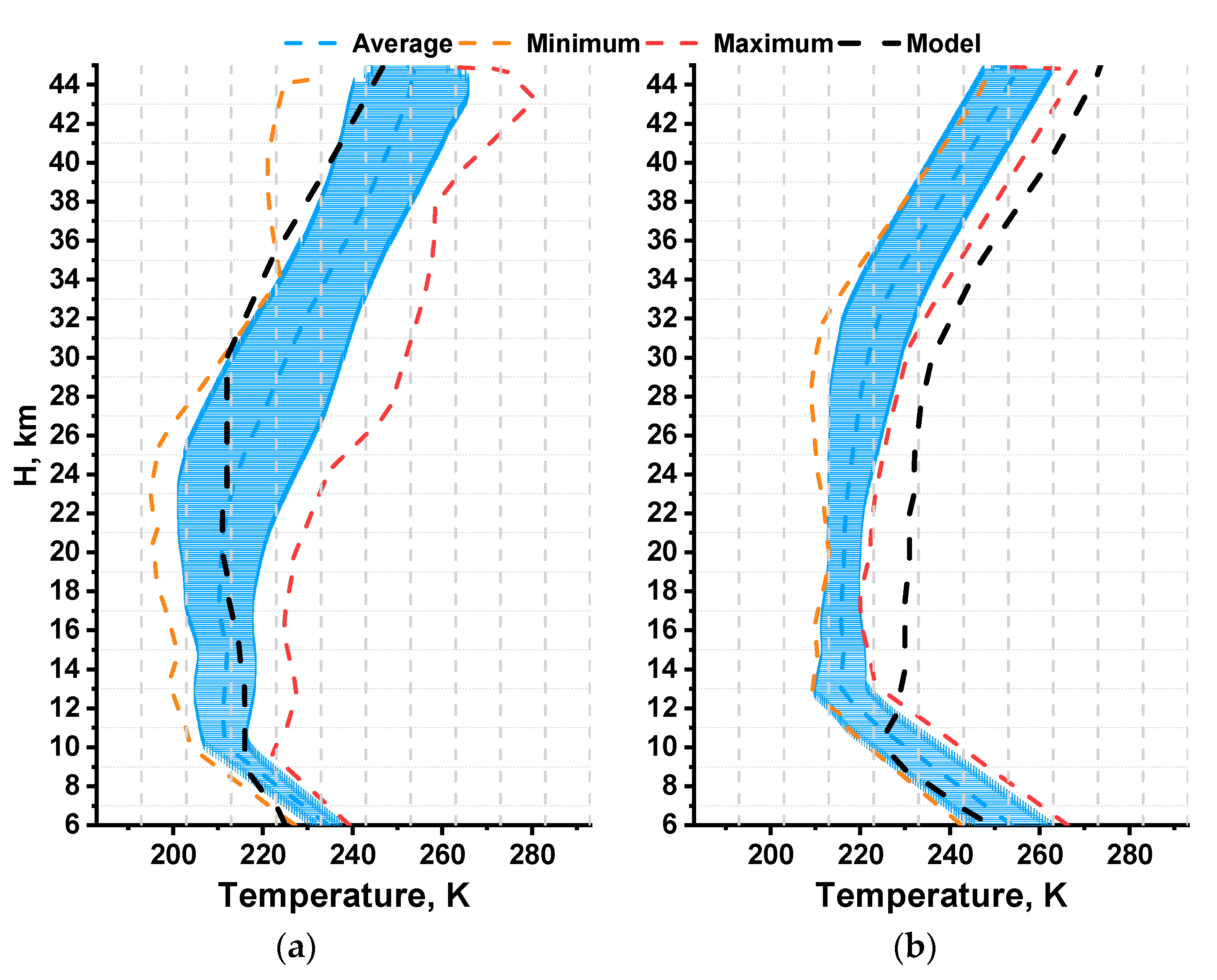
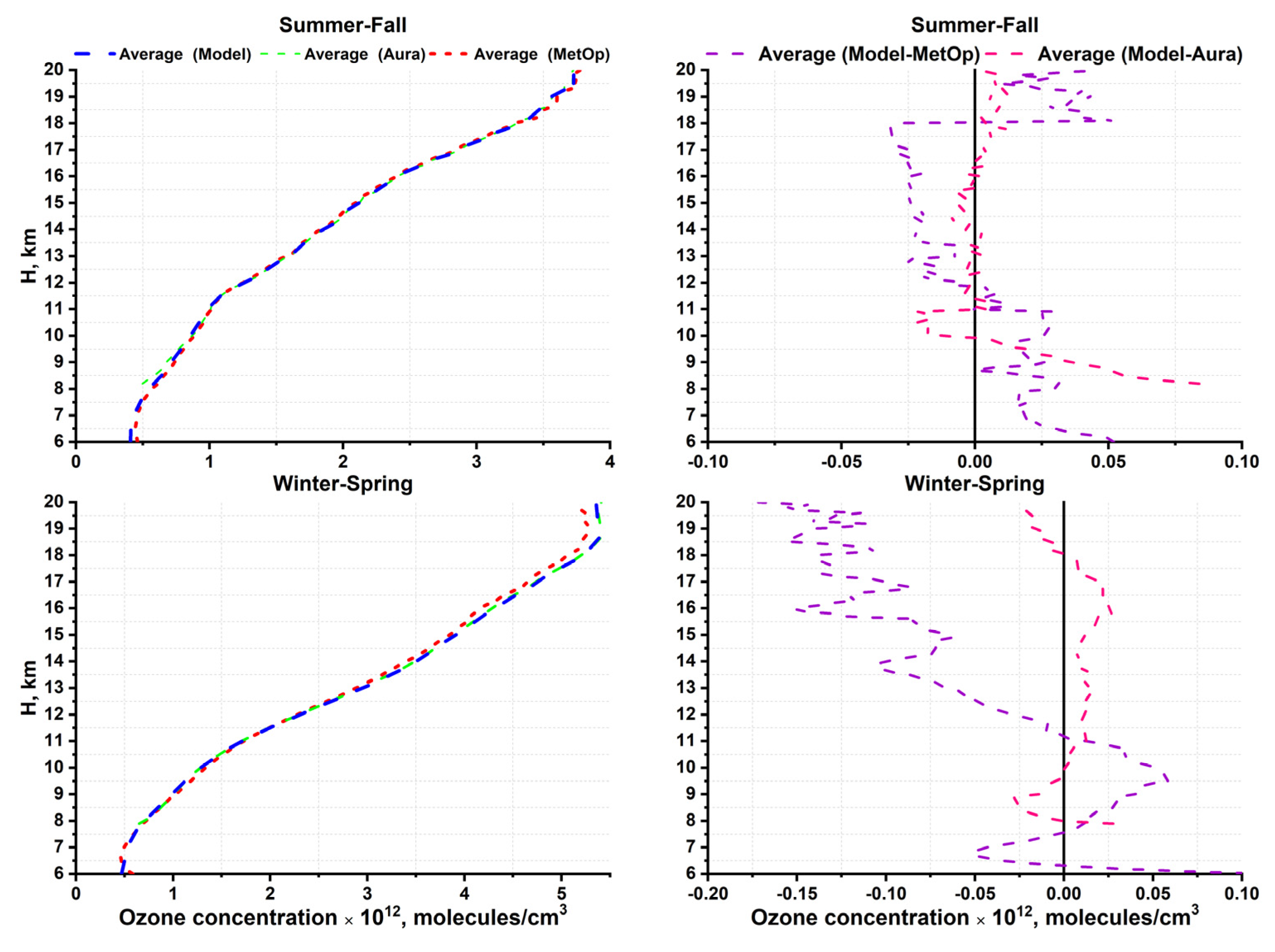
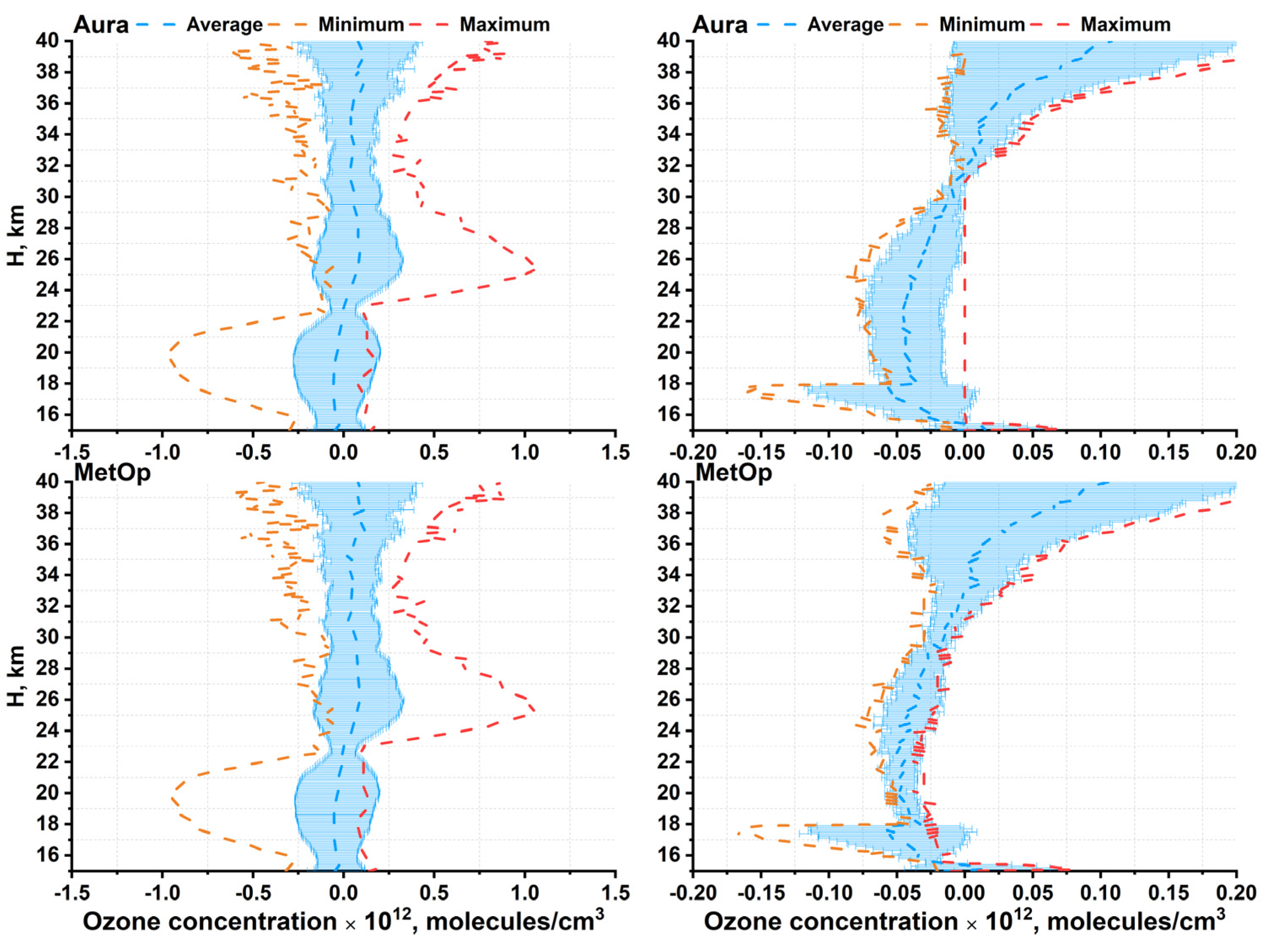
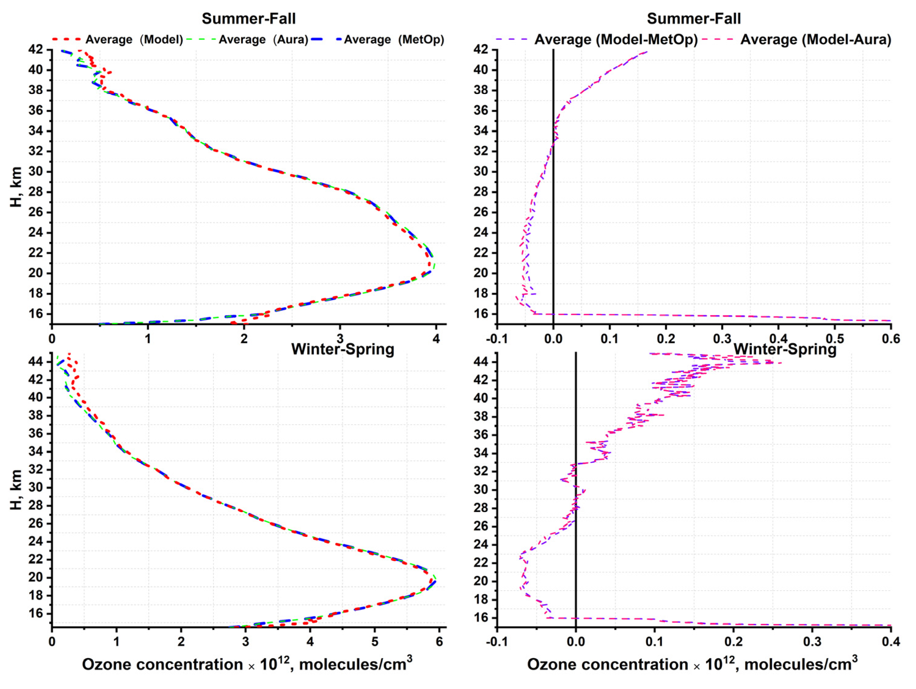
4. Measurement Results and Discussion

During 2018 we carried out 81 measurements of stratospheric OVD; and 79 measurements were performed in the upper troposphere–lower stratosphere. In this work, we used 25 measurements selected for analysis. By using the differential absorption and scattering method, with the real temperature measurements from MetOp and Aura satellites being input to the retrieval algorithm, as well as with the model values, we obtained a set of ozone profiles for the stratosphere and the upper troposphere–lower stratosphere. An analysis of the space-time comparison of lidar and satellite measurements was carried out by us in our previous work [7].
For analysis, we singled out two seasonal periods in lidar and satellite annual measurements of ozone vertical distribution: “winter–spring” (November–April) and “summer–fall” (May–October). A characteristic feature of winter–fall period is that large ozone concentrations are observed at the altitudes of the stratosphere and upper troposphere as compared to the summer–fall period. This is because of the meridional transport of cold air masses from the pole in the winter period.
Figure 2 presents the seasonal variations of Aura profiles of temperature over the entire study period, presented in our previous work [7], in comparison with the IAO model of temperature. Figure 3 presents the variations of MetOp profiles of temperature in comparison with the IAO model of temperature.
In Figure 2 and Figure 3, grey horizontal lines show temperature points of absorption cross-sections, intersecting the variations of temperature profiles. The numbers of points, which define the temperature profiles, are different for Aura and MetOp data. In the altitude range from about 0.1 to 45 km, there are just 35 points in Aura profiles and 91 points in MetOp profiles; it should also be remembered that temperature rapidly increases in Aura profiles below 8 km. Thus, the meteorological data from the MetOp satellite reflect more realistically the actual temperature of the atmosphere. The IASI data in the lower stratosphere and troposphere have a better spatial resolution than those from the Aura satellite; also, the number of points, which describe the temperature profile, is about 3 times larger. It can be concluded that IASI data provide more detailed behavior of the temperature in the study period. The strong differences between the satellite profiles of temperature and the model are associated with the divergence of the number of samples, compiled to create the model, as compared to the presented experimental dataset. However, this rather improves, than degrading, the result of the study because the deviations became more distinct. From Figure 2 and Figure 3 it can be seen that the number of crossings with respect to temperature points of the set [16,17] increases above the altitudes of 20–23 km, at which the ozone maximum is recorded over Tomsk; that is, the major part of the set of cross-sections, available for retrievals, is employed above these altitudes. We especially note that strong differences between the summertime temperature model and satellite data exist above 10 km.
Figure 4, Figure 5, Figure 6 and Figure 7 clearly demonstrate the effect of temperature correction, performed using Aura/MetOp data [23] and the IAO model with respect to season, as well as the difference, in absolute values, between OVDs, retrieved using model meteorological parameters [32] and satellite data.
Figure 4 and Figure 5 clearly illustrate the effect of temperature correction, carried out using meteorological data from Aura/MetOp satellites and IAO model of temperature, as well as the difference, in absolute values, between average OVDs over all days of measurements, retrieved using model meteorological parameters (“Model”) [32] and satellite data. The difference is denoted as “Model-MetOp” and “Model-Aura”. The discrepancies or differences between average ozone profiles, retrieved using temperature model and satellite data, are about the same. However, due to the shortage of measurements in summer–fall period according to the used data from work [7], these differences were more marked.
In Figure 4 and Figure 5 we can see the difference between the average lidar-derived ozone profiles, which were calculated using temperature profiles from satellites and model values for the study period. As can be seen, they are insignificant and within the range of ozone profile retrieval error: within 6% for the altitude range of 15–45 km and 7.2–18.5% for the altitude range of 5–20 km. The variations are more marked and significant in a particular case in Figure 6 and Figure 7.
We will analyze in detail the variations of the difference between all ozone profiles, retrieved using model- and satellite-derived temperatures. The differences between the profiles are reduced to the common altitude range of 16–40 km and 6–20 km for Figure 6 and Figure 7. From Figure 6 and Figure 7 it can be seen that, for the entire period of observations, a number of profiles exhibit underestimated and overestimated ozone concentrations during the summer–fall and winter–spring seasons relative to zero, because of a certain divergence between temperature profiles and temperature model.
From the analysis of field data on stratospheric OVD for the entire study period of 2018, presented in our previous work [7], we can draw the following conclusions. An insignificant difference between concentration profiles (Figure 4, Figure 5, Figure 6 and Figure 7), obtained using lidar and meteorological data from Aura and MetOp satellites, is present in the entire altitude range relative to zero. As a consequence, the average difference (Ozone profile (Temperature model)–Ozone profile (Aura temperature)) or deviation in ozone concentration for all days of measurements varies in the stratosphere from −0.06 × 10¹² molecules × cm−3 at a height of 17.4 km to 0.12 × 10¹² molecules × cm−3 at 38.2 km during winter–spring season, and from −0.05 × 10¹² molecules × cm−3 at height of 17.8 km to 0.1 × 10¹² molecules × cm−3 at 40 km during summer–fall season. For all profiles, the maximal deviation in the stratosphere is from 0.08 × 10¹² molecules × cm−3 at height of 17.4 km to 1.05 × 10¹² molecules × cm−3 at 25.3 km during winter–spring season, and from 0 × 1012 molecules × cm−3 at height of 15.5 km to 0.27 × 10¹² molecules × cm−3 at 40 km during summer–fall season. For all profiles, the minimal deviation in the stratosphere varies from −0.97 × 10¹² molecules × cm−3 at 19.7 km to −0.06 × 10¹² molecules × cm−3 at height of 25.3 km during winter–spring season, and from −0.16 × 10¹² molecules × cm−3 at height of 17.4 km to 0 × 1012 molecules × cm−3 at 31.8 km during summer–fall season. The average difference (Ozone profile (Temperature model)–Ozone profile (MetOp temperature)) or deviation in ozone concentration for all days of measurements varies in the stratosphere from −0.06 × 10¹² molecules × cm−3 at height of 17.4 km to 0.12 × 10¹² molecules × cm−3 at 38.2 km during winter–spring season, and from −0.06 × 10¹² molecules × cm−3 at height of 17.4 km to 0.1 × 10¹² molecules × cm−3 at 40 km during summer–fall season. For all profiles, the maximal deviation in the stratosphere is from 0.07 × 10¹² molecules × cm−3 at height of 17.4 km to 1.05 × 10¹² molecules × cm−3 at 25.3 km during winter–spring season, and from −0.04 × 10¹² molecules × cm−3 at height of 20.1 km to 0.27 × 10¹² molecules × cm−3 at 40 km during summer–fall season. For all profiles, the minimal deviation in the stratosphere varies from −0.95 × 10¹² molecules × cm−3 at 19.7 km to −0.05 × 10¹² molecules × cm−3 at height of 29.3 km during winter–spring season, and from −0.17 × 10¹² molecules × cm−3 at height of 17.4 km to −0.02 × 10¹² molecules × cm−3 at 15 km during summer–fall season. In an analogous way, the deviations in absolute values for all days of measurements with respect to seasons are presented in ozone concentrations in Table 2.
Thus, from analysis it follows that in the stratosphere, the differences may reach the absolute values of ozone concentration due to the use of satellite-based temperature in profile retrievals in the range from −0.97 × 10¹² molecules × cm−3 at 19.7 km to 1.05 × 10¹² molecules × cm−3 at 25.3 km during winter–spring season, and from −0.17 × 10¹² molecules × cm−3 at height of 17.4 km to 0.27 × 10¹² molecules × cm−3 at 40 km during summer–fall season.
However, the average deviations have insignificant values from −0.06 × 10¹² molecules × cm−3 at height of 17.4 km to 0.12 × 10¹² molecules × cm−3 at 38.2 km during winter–spring season, and from −0.06 × 10¹² molecules × cm−3 at height of 17.4 to 0.1 × 10¹² molecules × cm−3 at 40 km during summer–fall season.
Analogously, in the troposphere, the differences may reach the absolute values of ozone concentrations due to the use of satellite temperatures in profile retrievals in the range from −1.95 × 10¹² molecules × cm−3 at 18.6 km to 1.23 × 10¹² molecules × cm−3 at 18.2 km during winter–spring season, and from −0.15 × 10¹² molecules × cm−3 at height of 11.4 km to 0.3 × 10¹² molecules × cm−3 at 8 km during summer–fall season.
That large values are associated with the sample for separate days of observations, namely, with the altitude range of a single profile retrieved. The average deviations in the troposphere have insignificant values, from −0.22 × 10¹² molecules × cm−3 at height of 20 km to 0.11 × 10¹² molecules × cm−3 at 6 km during winter–spring season, and from −0.15 × 10¹² molecules × cm−3 at height of 7.8 to 0.14 × 10¹² molecules × cm−3 at 8 km during summer–fall season.
We note that the main variability range is nearly the same for the deviations calculated. A set of absorption cross-sections with a smaller step between temperature points should be obtained to record the significant differences between OVD profiles, retrieved using Aura/MetOp and the model temperatures.

5. Conclusions

The lidar complex at Siberian Lidar Station of IAO SB RAS was used to measure OVD together with the Aura and MetOp data in the upper troposphere–stratosphere in the altitude range ~5–45 km at sensing wavelengths of 299/341 and 308/353 nm.
Analysis of the difference between the profiles, retrieved using satellite data and temperature model, showed that the average deviations of the profiles of ozone concentration in the stratosphere are insignificant in value: from −0.06 × 10¹² molecules × cm−3 at height of 17.4 km to 0.12 × 10¹² molecules × cm−3 at 38.2 km during winter–spring season, and from −0.06 × 10¹² molecules × cm−3 at height of 17.4 to 0.1 × 10¹² mol. × cm−3 at 40 km during summer–fall season. Analogously, in the troposphere, the average deviations are: from −0.22 × 10¹² molecules × cm−3 at height of 20 km to 0.11 × 10¹² molecules × cm−3 at 6 km during winter–spring season, and from −0.15 × 10¹² molecules × cm−3 at height of 7.8 km to 0.14 × 10¹² molecules × cm−3 at 8 km during summer–fall season. We note that all variability range is nearly the same for the deviations calculated. The results of the analysis show that the apply of actual temperature correction using satellite temperature profiles makes it possible to increase the information content of lidar ozone sensing in the long-term monitoring at the pairs of wavelengths 299/341 nm and 308/353 nm. A set of absorption cross-sections with a smaller step between temperature points should be applied to record significant differences between OVD profiles, retrieved using Aura and MetOp temperature data. It should be noted that in this work we present the obtained deviations in absolute values, which is sufficient to estimate an insignificant effect of temperature correction at stratospheric altitudes and a more marked effect at altitudes of troposphere around the tropopause.

Author Contributions

Conceptualization, S.D., A.V.N., A.A.N. and O.K.; methodology, A.V.N. and A.A.N.; validation, A.A.N. and A.V.N.; formal analysis, A.A.N.; resources, A.V.N., S.D., Y.G. and A.A.N.; data curation, A.V.N., S.D., Y.G. and A.A.N.; writing—original draft preparation, A.A.N.; writing—review and editing, A.A.N.; visualization, A.A.N.; supervision, A.A.N.; project administration, A.A.N. All authors have read and agreed to the published version of the manuscript.

Funding

The work was financially supported in part by the President of the Russian Federation (scholarship for the support of young scientists and post-graduate students SP-3926.2018.3), the Ministry of Science and Higher Education of the Russian Federation (grant No. 075-15-2020-787 for implementation of large scientific project "Fundamentals, methods and technologies for digital monitoring and forecasting of the environmental situation on the Baikal natural territory") and the project No. AAAA-A17-117021310145-6 (in terms of obtaining measurement results).

Acknowledgments

The authors wish to thank I.V. Ptashnik, director of theV.E. Zuev Institute of Atmospheric Optics of the Siberian Branch of the Russian Academy of Science.

Conflicts of Interest

The authors declare no conflict of interest.

References

  1. Weitkamp, C. Lidar: Range Resolved Optical Remote Sensing of the Atmosphere; Springer: Berlin/Heidelberg, Germany, 2005; pp. 1–18. [Google Scholar]
  2. Liu, X.; Chance, K.; Sioris, C.E.; Kurosu, T.P. Impact of using different ozone cross sections on ozone profile retrievals from Global Ozone Monitoring Experiment (GOME) ultraviolet measurements. Atmos. Chem. Phys. 2007, 7, 3571–3578. [Google Scholar] [CrossRef] [Green Version]
  3. Orphal, J.; Staehelin, J.; Tamminen, J.; Braathen, G.; De Backer, M.-R.; Bais, A.; Balis, D.; Barbe, A.; Bhartia, P.K.; Birk, M.; et al. Absorption cross-sections of ozone in the ultraviolet and visible spectral regions: Status report 2015. J. Mol. Spectrosc. 2016, 327, 105–121. [Google Scholar] [CrossRef] [Green Version]
  4. Liu, C.; Liu, X.; Chance, K. The impact of using different ozone cross sections on ozone profile retrievals from OMI UV measurements. J. Quant. Spectrosc. Radiat. Transf. 2013, 130, 365–372. [Google Scholar] [CrossRef]
  5. Lamsal, L.N.; Weber, M.; Tellmann, S.; Burrows, J.P. Ozone column classified climatology of ozone and temperature profiles based on ozonesonde and satellite data. J. Geophys. Res. 2004, 109, D20304. [Google Scholar] [CrossRef]
  6. Wang, H.; Chai, S.; Tang, X.; Zhou, B.; Bian, J.; Zheng, X.; Vomel, H.; Yu, K.; Wang, W. Application of temperature dependent ozone absorption cross-sections in total ozone retrieval at Kunming and Hohenpeissenberg stations. Atmos. Environ. 2019, 215, 116890. [Google Scholar] [CrossRef]
  7. Burlakov, V.D.; Dolgii, S.I.; Nevzorov, A.A.; Nevzorov, A.V.; Gridnev, Y.; Kharchenko, O.V. Measurements of Ozone Vertical Profiles in the Upper Troposphere–Stratosphere over Western Siberia by DIAL, MLS, and IASI. Atmosphere 2020, 11, 196. [Google Scholar] [CrossRef] [Green Version]
  8. Park, C.B.; Nakane, H.; Sugimoto, N.; Matsui, I.; Sasano, Y.; Fujinuma, Y.; Ikeuchi, I.; Kurokawa, J.-I.; Furuhashi, N. Algorithm improvement and validation of National Institute for Environmental Studies ozone differential absorption lidar at the Tsukuba Network for Detection of Stratospheric Change complementary station. Appl. Opt. 2006, 45, 3561–3576. [Google Scholar] [CrossRef]
  9. Nakazato, M.; Nagai, T.; Sakai, T.; Hirose, Y. Tropospheric ozone differential-absorption lidar using stimulated Raman scattering in carbon dioxide. Appl. Opt. 2007, 46, 2269–2279. [Google Scholar] [CrossRef]
  10. Godin, S.; Bergeret, V.; Bekki, S.; David, C.; Mégie, G. Study of the interannual ozone loss and the permeability of the Antarctic Polar Vortex from long-term aerosol and ozone lidar measurements in Dumont d’Urville (66.4°, 140°S). J. Geophys. Res. 2001, 106, 1311–1330. [Google Scholar] [CrossRef]
  11. Gaudel, A.; Ancellet, G.; Godin-Beekmann, S. Analysis of 20 years of tropospheric ozone vertical profiles by lidar and ECC at Observatoire de Haute Provence (OHP) at 44 N, 6.7 E. Atmos. Environ. 2015, 113, 78–89. [Google Scholar] [CrossRef]
  12. Hu, S.; Hu, H.; Wu, Y.; Zhou, J.; Qi, F.; Yue, G. Atmospheric ozone measured by differential absorptionlidar over Hefei. Proc. SPIE 2003. [Google Scholar] [CrossRef]
  13. Liu, X.; Zhang, Y.; Hu, H.; Tan, K.; Tao, Z.; Shao, S.; Cao, K.; Fang, X.; Yu, S. Mobile lidar for measurements of SO2 and 03 in the low troposphere. Proc. SPIE 2005. [Google Scholar] [CrossRef]
  14. McDermid, I.S.; Godin, S.M.; Lindquist, L.O. Ground-based laser DIAL system for long-term measurements of stratospheric ozone. Appl. Opt. 1990, 29, 3603–3612. [Google Scholar] [CrossRef] [PubMed]
  15. McDermid, I.S.; Beyerle, G.; Haner, D.A.; Leblanc, T. Redesign and improved performance of the tropospheric ozone lidar at the Jet Propulsion Laboratory Table Mountain Facility. Appl. Opt. 2002, 41, 7550–7555. [Google Scholar] [CrossRef]
  16. Steinbrecht, W.; McGee, T.J.; Twigg, L.W.; Claude, H.; Schönenborn, F.; Sumnicht, G.K.; Silbert, D. Intercomparison of stratospheric ozone and temperature profiles during the October 2005 Hohenpeißenberg Ozone Profiling Experiment (HOPE). Atmos. Meas. Tech. 2009, 2, 125–145. [Google Scholar] [CrossRef] [Green Version]
  17. Sullivan, J.T.; McGee, T.J.; Sumnicht, G.K.; Twigg, L.W.; Hoff, R.M. A mobile differential absorption lidar to measure sub-hourly fluctuation of tropospheric ozone profiles in the Baltimore–Washington, D.C. region. Atmos. Meas. Tech. 2014, 7, 3529–3548. [Google Scholar] [CrossRef] [Green Version]
  18. Pavlov, A.N.; Stolyarchuk, S.Y.; Shmirko, K.A.; Bukin, O.A. Lidar Measurements of Variability of the Vertical Ozone Distribution Caused by the Stratosphere–Troposphere Exchange in the Far East Region. Atmos. Ocean Opt. 2013, 26, 126–134. [Google Scholar] [CrossRef]
  19. Burlakov, V.D.; Dolgii, S.I.; Nevzorov, A.V. Modification of the measuring complex at the Siberian Lidar Station. Atmos. Ocean Opt. 2004, 17, 756–762. [Google Scholar]
  20. Dolgii, S.I.; Nevzorov, A.A.; Nevzorov, A.V.; Romanovskii, O.A.; Makeev, A.P.; Kharchenko, O.V. Lidar Complex for Measurement of Vertical Ozone Distribution in the Upper Troposphere–Stratosphere. Atmos. Ocean Opt. 2018, 31, 702–708. [Google Scholar] [CrossRef]
  21. Fang, X.; Li, T.; Ban, C.; Wu, Z.; Li, J.; Li, F.; Cen, Y.; Tian, B. A mobile differential absorption lidar for simultaneous observations of tropospheric and stratospheric ozone over Tibet. Opt. Express 2019, 27, 4126–4139. [Google Scholar] [CrossRef]
  22. Waters, J.W.; Froidevaux, L.; Harwood, R.S.; Jarnot, R.F.; Pickett, H.M.; Read, W.G.; Siegel, P.H.; Cofield, R.E.; Filipiak, M.J.; Flower, D.A.; et al. The Earth Observing System Microwave Limb Sounder (EOS MLS) on the Aura Satellite. IEEE TGRS Trans. Geosci. Remote Sens. 2006, 44, 1075–1092. [Google Scholar] [CrossRef]
  23. NASA (National Aeronautics and Space Administration). Microwave Limb Sounder. The MLS Temperature Product. Available online: https://mls.jpl.nasa.gov/products/temp_product.php (accessed on 31 August 2020).
  24. NASA (National Aeronautics and Space Administration). MLS Temperature Data. Available online: https://avdc.gsfc.nasa.gov/pub/data/satellite/Aura/MLS/ (accessed on 31 August 2020).
  25. August, T.; Klaes, D.; Schlüssel, P.; Hultberg, T.; Crapeau, M.; Arriaga, A.; O’Carroll, A.; Coppens, D.; Munro, R.; Calbet, X. IASI on Metop-A: Operational Level 2 retrievals after five years in orbit. J. Quant. Spectrosc. Radiat. Transf. 2012, 113, 1340–1371. [Google Scholar] [CrossRef]
  26. Matvienko, G.G.; Belan, B.D.; Panchenko, M.V.; Romanovskii, O.A.; Sakerin, S.M.; Kabanov, D.M.; Turchinovich, S.A.; Turchinovich, Y.S.; Eremina, T.A.; Kozlov, V.S.; et al. Complex experiment on studying the microphysical, chemical, and optical properties of aerosol particles and estimating the contribution of atmospheric aerosol-to-earth radiation budget. Atmos. Meas. Tech. 2015, 8, 4507–4520. [Google Scholar] [CrossRef] [Green Version]
  27. Measures, R.M. Laser Remote Sensing: Fundamentals and Applications; Reprint 1984 de Krieger Publishing Company; Krieger Publishing Company: Malabar, FL, USA, 1992; pp. 237–280. [Google Scholar]
  28. Burlakov, V.D.; Dolgii, S.I.; Nevzorov, A.A.; Nevzorov, A.V.; Romanovskii, O.A. Algorithm for Retrieval of Vertical Distribution of Ozone from DIAL Laser Remote Measurements. Opt. Mem. Neural Netw. Inf. Opt. 2015, 24, 295–302. [Google Scholar] [CrossRef]
  29. Dolgii, S.I.; Nevzorov, A.A.; Nevzorov, A.V.; Romanovskii, O.A.; Kharchenko, O.V. Intercomparison of Ozone Vertical Profile Measurements by Differential Absorption Lidar and IASI/MetOp Satellite in the Upper Troposphere–Lower Stratosphere. Remote Sens. 2017, 9, 447–462. [Google Scholar] [CrossRef] [Green Version]
  30. Gorshelev, V.; Serdyuchenko, A.; Weber, M.; Chehade, W.; Burrows, J.P. High spectral resolution ozone absorption cross-sections—Part 1: Measurements, data analysis and comparison with previous measurements around 293 K. Atmos. Meas. Tech. 2014, 7, 609–624. [Google Scholar] [CrossRef] [Green Version]
  31. Serdyuchenko, A.; Gorshelev, V.; Weber, M.; Chehade, W.; Burrows, J.P. High spectral resolution ozone absorption cross-sections—Part 2: Temperature dependence. Atmos. Meas. Tech. 2014, 7, 625–636. [Google Scholar] [CrossRef] [Green Version]
  32. Zuev, V.E.; Komarov, V.S. Statistical Models of the Temperature and Gaseous Components of the Atmosphere; Springer: Dordrecht, The Netherlands, 1987; p. 320. [Google Scholar]
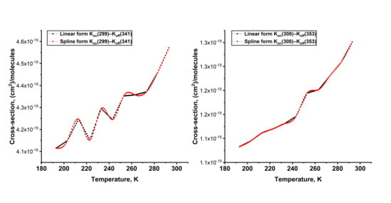
Figure 1. Cross-section difference for two-wavelength pairs in the linear and spline forms.
Atmosphere 11 01139 g001
Figure 2. Seasonal variations of Aura profiles of temperature in comparison with the Institute of Atmospheric Optics (IAO) model of temperature: (a) winter–spring variations; (b) summer–fall variations.
Atmosphere 11 01139 g002
Figure 3. Seasonal variations of MetOp profiles of temperature, in comparison with the IAO model of temperature: (a) winter–spring variations; (b) summer–fall variations.
Atmosphere 11 01139 g003
Figure 4. Average ozone vertical distributions (OVDs) (obtained at 308/353 nm) for different seasons, retrieved using model meteorological parameters and data from Aura and MetOp satellites in the stratosphere: (a) average ozone profiles; (b) average ozone profile (Temperature model)–average ozone profile (satellite temperature).
Atmosphere 11 01139 g004
Figure 5. Average OVDs (obtained at 308/353 nm) for different seasons, retrieved using model meteorological parameters and data from Aura and MetOp satellites in the stratosphere: (a) average ozone profiles; (b) average ozone profile (Temperature model)–average ozone profile (satellite temperature).
Atmosphere 11 01139 g005
Figure 6. Difference between profiles, retrieved using model meteorological parameters and data from Aura and MetOp satellites in the stratosphere: ozone profile (Temperature model)–ozone profile (satellite temperature), where (a) winter–spring period; (b) summer–fall period.
Atmosphere 11 01139 g006
Figure 7. Difference between profiles, retrieved using model meteorological parameters and Aura/MetOp data in the lower stratosphere and upper troposphere: ozone profile (Temperature model)—ozone profile (satellite temperature), where (a) winter–spring period; (b) summer–fall period.
Atmosphere 11 01139 g007
Table 1. The ozone absorption cross-sections (cm2) for the range 193–293 K at the wavelengths of ozone sensing [30,31].
Wavelength,
nm
Temperature, K
193203213223233243253263273283293
Online
2994.12
× 10−19
4.15
× 10−19
4.25
× 10−19
4.15
× 10−19
4.3
× 10−19
4.25
× 10−19
4.36
× 10−19
4.36
× 10−19
4.38
× 10−19
4.46
× 10−19
4.58
× 10−19
3081.13
× 10−19
1.14
× 10−19
1.16
× 10−19
1.17
× 10−19
1.18
× 10−19
1.19
× 10−19
1.24
× 10−19
1.25
× 10−19
1.28
× 10−19
1.31
× 10−19
1.35
× 10−19
Offline
3415.62
× 10−22
5.94
× 10−22
6.1
× 10−22
6.95
× 10−22
7.05
× 10−22
7.59
× 10−22
8.15
× 10−22
8.9
× 10−22
9.9
× 10−22
1.08
× 10−21
1.15
× 10−21
3534.95
× 10−23
6.4
× 10−23
7.25
× 10−23
8.88
× 10−23
9.57
× 10−23
1.1
× 10−22
1.27
× 10−22
1.45
× 10−22
1.67
× 10−22
2.02
× 10−22
2.38
× 10−22
Table 2. Differences between ozone profiles for the troposphere and two seasons: winter–spring and summer–fall.
Troposphere
Difference
×1012 Molecules/cm3
Difference
×1012 Molecules/cm3
Aura Temperature
Winter–SpringSummer–Fall
Minimumfrom −1.95 at 18.6 km
to −0.05 at 10.7 km
from −0.15 at 11.4 km
to 0.01 at 9.5 km
Maximumfrom 0.09 at 13.9 km
to 1.23 at 18.2 km
from −0.03 at 18.9 km
to 0.3 at 8 km
Averagefrom −0.22 at 20 km
to 0.05 at 9.8 km
from −0.04 at 19.5 km
to 0.14 at 8 km
MetOp Temperature
Winter–SpringSummer–Fall
Minimumfrom −1.95 at 18.6 km
to −0.08 at 10.5 km
from −0.88 at 7.8 km
to 0 at 8 km
Maximumfrom 0.07 at 13.9 km
to 2.11 at 6 km
from −0.02 at 19.4 km
to 0.16 at 6.2 km
Averagefrom −0.19 at 20 km
to 0.11 at 6 km
from −0.15 at 7.8 km
to 0.03 at 8.3 km
Publisher’s Note: MDPI stays neutral with regard to jurisdictional claims in published maps and institutional affiliations.

