Article

Assessing the Horizontal Homogeneity of the Atmospheric Boundary Layer (HHABL) Profile Using Different CFD Software

1
Civil and Architectural Engineering Department, College of Engineering, Applied Science University (ASU), Bahrain 5055, Bahrain
2
School of Engineering, London South Bank University, London SE1 0AA, UK
*
Authors to whom correspondence should be addressed.
Atmosphere 2020, 11(10), 1138; https://doi.org/10.3390/atmos11101138
Submission received: 6 September 2020 / Revised: 8 October 2020 / Accepted: 9 October 2020 / Published: 21 October 2020
(This article belongs to the Special Issue Atmospheric Modeling Study)

Abstract

:
One of the main factors affecting the reliability of computational fluid dynamics (CFD) simulations for the urban environment is the Horizontal Homogeneity of the Atmospheric Boundary Layer (HHABL) profile—meaning the vertical profiles of the mean streamwise velocity, the turbulent kinetic energy, and dissipation rate are maintained throughout the streamwise direction of the computational domain. This paper investigates the preservation of the HHABL profile using three different commercial CFD codes—the ANSYS Fluent, the ANSYS CFD, and the Siemens STAR-CCM+ software. Three different cases were considered, identified by their different inlet conditions for the inlet velocity, turbulent kinetic energy, and dissipation rate profiles. Simulations were carried out using the RANS k-ε turbulence model. Slight variations in the eddy viscosity models, as well as in the wall boundary conditions, were identified in the different software, with the standard wall function with roughness being implemented in the Fluent applications, the scalable wall function with roughness in the CFX applications, and the blended wall function option in the STAR-CCM+ simulations. There was a slight difference in the meshing approach in the three different software, with a prism-layer option in the STAR-CCM+ software, which allowed a finer mesh near the wall/ground boundary. The results show all three software are able to preserve the horizontal homogeneity of the ABL—less than 0.5% difference between the software—indicating very similar degrees of accuracy.

Graphical Abstract

1. Introduction

This work is part of a research project aiming to study the optimum mounting locations of roof-mounted wind turbines on isolated buildings using computational fluid dynamics (CFD), with the implementation of existing commercial CFD software. It is therefore crucial/important to investigate how different commercial software respond to the HHABL profile challenge. Numerical simulation methods, including computational fluid dynamics (CFD), is one of the primary assessment tools for urban physics [1]. CFD simulations enable investigations of air pollution dispersion within the built environment [2], assessment of the wind potentials for wind turbines [3,4] and their integration within the built environment [5], and pedestrian-level wind speed for wind comfort assessment [6], as well as high-resolution predictions of the urban microclimate and thermal comfort [7]. Thus, CFD simulation can be used as a tool for informed decision-making in urban design applications [8]. However, CFD simulations are embedded with errors and uncertainties linked with the numerical diffusion due to grid resolution and numerical solvers implemented, as well as accurate representation and capturing of atmospheric turbulence. Thus, best practice guidelines should be consulted before running CFD simulations [9]. In addition, the consistency and accuracy of CFD simulations may be compromised by the Horizontal Homogeneity of the Atmospheric Boundary Layer (HHABL) profile throughout the computational domain, meaning that no streamwise gradients in the flow variables in the flow direction from the inlet boundary throughout the domain to the outlet boundary should be observed when modelling an empty domain [10,11]. It is evident that simulating a HHABL profile is difficult and requires careful consideration of the boundary conditions [11,12,13]. Certain CFD studies [14,15] have shown that the approach flow changed rapidly in the upstream region of the computational domain, with a considerable acceleration of the flow near the surface. The effect of inappropriate top boundary conditions on the homogeneity problem was also investigated in [16], indicating that not only the inflow conditions can be responsible for the inhomogeneity but, also, other boundary conditions.
Several studies have been carried out using the standard k–ε turbulence model [17,18] with the standard wall functions without roughness modification and reporting an unwanted change in the profiles of mean wind speed and, especially, turbulent kinetic energy. The simulation results led to discrepancies between CFD predictions and the corresponding wind tunnel measurements, and these discrepancies were believed to be due to the wall boundary conditions. The effect of the wall boundary conditions and wall roughness on the ABL profiles was also extensively discussed in [19,20]. A similar problem for the preservation of the inlet turbulent kinetic energy profile was reported in [21] using the ANSYS CFX-4.1 software, whilst the implementation of the Fluent software was discussed in [22], where the authors considered two turbulence models: (i) the standard k–ε model and (ii) the Reynolds stress model (RSM). The authors observed significant profile changes in an empty computational domain, especially for the turbulent kinetic energy. Problems in simulating a horizontally homogeneous ABL flow were also reported by [23] using the CFX-5 software and by [24,25,26], who all implemented the Fluent 5 and Fluent 6 software versions. The importance of correctly reproducing the atmospheric boundary layer (ABL) profile in CFD simulations, in addition to maintaining the profile throughout the streamwise direction of the computational domain, was also clearly asserted in [27,28,29], the authors highlighted the fact that the boundary conditions should be adjusted to produce a horizontally homogenous boundary layer flow in the absence of any obstructions.
The preceding literature indicates how the accuracy in simulating the ABL flow in the computational domain is imperative to obtain accurate and reliable predictions of related atmospheric processes, particularly processes related to air pollution dispersion and thermal comfort. This paper aims to investigate the horizontal homogeneity of the HHABL profile using three commercial CFD software, namely ANSYS Fluent [30], ANSYS CFX [31], and STAR CCM++ [32], in an empty domain. Initially, the same simulation conditions are considered in all three software, but these progressively change slightly to achieve the HHABL profile in each separately. Slight variations exist amongst the three software—in the Fluent and STAR-CCM+ software, the Realizable k–ε model was used, whilst the standard k–ε model was implemented in the CFX software (due to the absence of a realizable model option). With regards to the wall boundary conditions, the standard wall function was used in Fluent, whereas, in the CFX, the scalable wall function was used instead. In the STAR CCM+ software, the blended wall function option was implemented.
Although, as indicated above, substantial work has already been done in this field by several researchers, a detailed comparison between different CFD software has not yet been published. It is therefore the aim of this work to assess the HHABL profile using three commercial software (Fluent, ANSYS CFX, and Siemens STAR-CCM+) and the parameters associated with them. The work was based on previous research [10], which looked at differences between simulated outlet and inlet profiles only using the ANSYS Fluent software. The same computational domain was used in our study, with the additional testing of two other commercial software—these being the ANSYS CFX and the Siemens STAR-CCM+ software. We also carried out a statistical analysis of the differences between the downstream profiles and the inlet—something that was not included in [10] or in any other literature. The work is presented as follows: Section 2 presents the governing equations associated with the Reynolds-Averaged Navier Stokes (RANS) and the k–ε models, together with the computational set-up and boundary conditions. Section 3 presents the computational results for the different scenarios investigated, using the three different software, whilst Section 4 discusses the differences and summarizes the conclusions.

2. Methodology

Our aim was to assess the capability of the three different softwares in achieving the HHABL profile. The unintended differences between inlet profiles and downstream/incident profiles (i.e., the horizontal homogeneity problem) can be detrimental for the success of any CFD simulation for urban applications, given that even minor changes to the incident flow profiles can cause significant changes in the turbulent flow field. To quantify the possible deviation from the horizontal homogeneity of the atmospheric air boundary layer, the CFD results for the vertical profiles of the streamwise—x-direction) velocity (u) turbulent dissipation rate (TDR), ε, and turbulent kinetic energy (TKE), k, at four locations (L2, L3, L4, and L5) downstream (x-direction) the inlet and through the center of an empty computational domain are considered in comparison to the inlet profiles. The x coordinates of each location are shown in Figure 1, with L1 being the inlet (x = 0, L2 − x = 31.5 m, L3 − x = 63 m, and L4 − x = 94.5 m) and L5 − x= 126 m the outlet. All locations run through the middle of the domain with a y-coordinate value of 18 m.
For each j location, with j denoting the downstream lines L2, L3, L4, and L5, the statistical measure—mean absolute percentage error (MAPE)—quantifying the error/difference between two data sets was determined. Our two data sets comprised: (i) the inlet vertical profile of each parameter of interest (e.g. velocity, TDR, or TKE) (1st data set) and (ii) the vertical profile of these parameters at the other locations Lj—with j varying from 2 to 5) (2nd data set). Thus, MAPE(p, j)—representing the MAPE for parameter p at location j—was estimated as follows:
M A P E ( p , j ) = 1 n i = 1 n = 72 | Y i p , j Y i p , 1 Y i p , 1 | 100  
where i represents each data point on the vertical profile—a total of 72 data points on each profile—thus, n = 72; j represents the downstream locations of interest, e.g., lines L2, L3, L4, and L5; p represents the different parameters of interest, e.g., p = 1 represents velocity; p = 2 represents TDR, and p = 3 represents TKE;   Y i p , j represents the parameter value of each point i of the vertical profile at each j location; and, finally, Y i p , 1 are the parameter values of each point i of the vertical profile at the inlet (j = 1, i.e., line L1).
To incorporate all the possible variations between the MAPEs in all three software, we considered the overall mean MAPE(p,j) over all parameters and all locations—for each software—which is defined as the Q-factor; this was estimated as follows:
Q ( % ) = 1 3 p = 1 3 1 4 j = 2 5 M A P E ( p , j )
To assist in identifying the source/s of the slight variations in the HHABL observed in the different software, we compared the following aspects of the models/simulations.
  • The transport equations for the turbulent kinetic energy and dissipation rate for the three different software and the differences between them.
  • The differences—if any—between the various constants.
  • The boundary conditions necessary to achieve homogeneity in the different software, e.g., (i) ground boundary conditions/wall functions, (ii) boundary conditions, and (iii) outlet boundary conditions. The inlet conditions were the same in all software and in all cases tested.
  • The numerical solvers and meshing options for each case.
All aspects are addressed and discussed in more detail in the following sections.

2.1. Theoretical Background

Governing Equations

Representing turbulence in the RANS momentum equations requires a turbulent eddy viscosity model. The k–ε transport equations have traditionally been implemented to determine the turbulent eddy viscosity with many modifications over the years. One of the most representative k–ε models is the realizable k–ε model, which involves a new transport equation for the dissipation rate and is recommended for studying similar cases as outlined in the introduction. The two main advantageous characteristics of the realizable k–ε model are: (a) the introduction of a variable damping function dependent on the mean flow turbulent properties in the critical model coefficient C μ and (b) the mathematical constraints applied to the normal stresses, so that the physics of the turbulence can be captured more accurately. We applied the realizable model in both the Fluent and STAR-CCM+ software; however, this option is currently not available in the ANSYS CFX software, and hence, the standard k–ε model was implemented instead. In all cases, the simplified k-ε transport equations are considered, where buoyancy and compressibility effects are considered negligible. The general RANS equations (mass continuity, momentum, and energy) for an incompressible fluid—with buoyancy effects negligible—are initially given, followed by the corresponding k-ε transport equations, for each software.
(a)
RANS Equations
The steady, time-averaged (mean) mass continuity and momentum equations for an incompressible fluid, with negligible buoyancy effects, are given by Equations (3) and (4) further below:
u i ¯ x i =   0
x j ( u j ¯   u i ¯ ) = P ¯ x i + x j ( 2 μ S i j + τ i j )
where ρ is the fluid density, and u i ¯ is the mean (time-averaged) velocity field; note that the velocity field u i is composed of the mean component u i ¯ and fluctuating component u i , and, thus, is given by the expression u i = u i ¯ + u i . When time-averaged, u i becomes the same as the mean component, since the time-averaged fluctuating component is zero, i.e., u i ¯ = 0, P ¯ is the mean fluid pressure, S i j is the mean strain-rate tensor given by S i j = 1 2 ( u i x j + u j x i ) , and μ is the dynamic viscosity of the fluid, whilst τ i j is the additional stress tensor due to turbulence, also known as the Reynolds stress tensor; this term is added to the original momentum equation, and it is related to the turbulent eddy viscosity μ t . The momentum equation, Equation (4), is also often seen in the following form:
u i ¯ t + x j ( u j ¯ u i ¯ ) = P ¯ x i + μ 2 u j ¯ x i x j + τ i j x j
Determining the additional stress tensor τ i j is one of the greatest challenges in turbulence modelling for capturing accurately the turbulence effects; traditionally, two methods have been considered by researchers: (a) the eddy viscosity method and (b) the Reynolds stress transport equation. In our current work, we consider the eddy viscosity approach in determining the turbulent stress tensor term τ i j . It is usually given by the expression:
τ i j = u i u j ¯ = 2 μ t S i j 2 3 k δ i j
where μ t is the turbulent eddy viscosity, k is the turbulent kinetic energy, and δ i j is the Kronecker delta function. The different eddy viscosity models within the different software are given in the following subsections.
(b)
Eddy Viscosity Models
(i) Fluent and CFX software
The eddy viscosity within both the Fluent and CFX software is obtained from the following expression:
μ t =   C μ ρ k 2 ε
where k is the turbulent kinetic energy, and ε is the turbulent dissipation rate. The parameter C μ is obtained from the following expression: C μ =   1 A 0 + A S   k U ε   , where, when ignoring rotational effects, U depends on the strain-rate tensor components as follows:
U   S i j   S i j
The model constants A 0 and A S are estimated through the expressions: A 0 = 4.04 and A S =   6   c o s φ , where φ   =   1 3   cos 1 6   W , W = S i j S j k S k i S ˜ 3 , and S ˜ = 2 S i j S i j . Within the CFX software, the C μ is a constant, with a default value of C μ = 0.09 . The overall effective viscosity is given by μ e f f = μ + μ t .
(ii) STAR-CCM+ software
Slightly different to the above two software, the eddy viscosity μ t within the STAR-CMM+ software is given by the expression:
μ t =   ρ C μ f μ k T
where ρ is the fluid density, and f μ is a complex damping function [32]. k is the turbulent kinetic energy, and T is the turbulent time scale. The parameter C μ is a model coefficient and, as in the CFX software, has the value of 0.09. The eddy viscosity μ t is required for determining the stress tensor component due to turbulence, τ i j , given by the earlier expression—Equation (6).
The above expressions show the slight variations between the eddy viscosity modes implemented within the Fluent, CFX, and STAR-CCM+ software [30,31,32].
(c)
Transport equations for the turbulent kinetic Energy k and dissipation rate
(i) ANSYS Fluent
t   ( ρ k ) + x j ( ρ k u j ) = x j [ ( μ + μ t σ k ) k x j ] + G k   ρ ε
t ( ρ ε ) + x j ( ρ ε u j   ) = x j [ ( μ + μ t σ ε ) ε x j ] ρ C 2 ε 2 k
The production term G k   in Equation (11) is given by the expression: G k   = μ t S ˜ 2 , where S ˜ = 2 S i j S i j , whilst the parameter C 2 in Equation (10) has the value of 0.9.
(ii) ANSYS CFX
( ρ k ) t + x j ( ρ u j   ¯ k ) = x j [ ( μ + μ t σ k ) k x j ] + P k ρ ε
( ρ ε ) t + x j ( ρ u j ¯ ε ) = x j [ ( μ + μ t σ ε ) ε x j ] + ε k ( C ε 1 P k C ε 2 ρ ε )
where C ε 1 , C ε 2 , σ k , and σ ε are constants (see Table 1), and P k is turbulence production term given by:
P k =   μ t ( u i ¯ x j + u j ¯ x i ) u i ¯ x j 2 3 u k ¯ x k [ 3 μ t u k ¯ x k + ρ k ]
The values of the parameters C ε 1 and C ε 2 are given in Table 1. To avoid the build-up of turbulent kinetic energy in stagnation regions, two production limiters are available, as reported in the CFX manual [31]. The k–ε standard model with the scalable wall function was implemented within the CFX software, which virtually moves the first computational node to be outside the viscous sublayer [31].
(iii) Siemens STAR-CCM+ software
The general transport equations are given by:
t ( ρ k ) +   ·   ( ρ k u ¯ ) =   ·   [ ( μ + μ t σ k ) k   ] + P k ρ ( ε ε o ) + S k
t ( ρ ε ) +   ·   ( ρ ε u ¯ ) =   ·   [ ( μ + μ t σ ε ) ε   ] + 1 T e C ε 1 P ε C ε 2 f 2 ρ ( ε T e ε o T o ) + S ε
where ρ is the fluid density, u ¯ is the mean velocity, μ is the dynamic viscosity of the fluid, μ t is the turbulent eddy viscosity, P k and P ε are the production terms for the turbulent kinetic energy k and dissipation rate ε , respectively, f 2 is the damping function given by the expression f 2 =   k k + v ε , and S k and S ε are user-defined source terms, which, in our cases, are eliminated. The remaining parameters, σ k , σ ε , C ε 1 , and   C ε 2 are model coefficients, as shown in Table 1.
For the realizable k ε model, the production term for the kinetic energy k , after assuming the compressibility and buoyancy effects are negligible, is given by the expression:
P k =   f c G k
where f c is a curvature correction factor, incorporating the effects of local rotation and vorticity rates which influence the production rate of the turbulent kinetic energy. The term G k is the turbulent production given by:
G k = μ t S ˜ 2   2 3 ρ k ·   ( u ¯ ) 2 3 μ t ( ·   ( u ¯ ) ) 2
The above expression is the same one as used in the CFX software, whilst the Fluent expression contains only the first term of the right hand side expression, i.e., only the μ t S 2 term. The production term P ε for the turbulent dissipation rate is related to the P k term through the equation:
P ε =   f c S ˜ P k
where S ˜ is the modulus of the mean strain tensor S given by S = 1 2 ( u ¯ + u ¯ T ) .

2.2. Computational Aspects

2.2.1. Computational Domain and Meshing

The 3D computational domain considered in this work is shown in Figure 1 and its dimensions are as follows: Length (x-direction)—126 m, width (y-direction)—36 m, and height (z-direction)—36 m. The locations where the vertical profiles of the three parameters (streamwise velocity, u; turbulent kinetic energy, k; and turbulent dissipation rate, ε) were compared against the inlet profile at L1 are also shown in Figure 1. The initial conditions for the parameters of interest (u; turbulent kinetic energy, k; and turbulent dissipation rate, ε) were based on the their values for the inlet conditions, i.e., the computational domain was initialized using the inlet values of these three parameters, whilst pressure was initialized to the atmospheric pressure value.
(i)
Fluent and CFX meshing options
The mesh used in both Fluent and CFX are an equidistant structured mesh with spacing of 0.5m in the X, Y, and Z directions, giving a total of 1,306,368 hexahedral cells. Figure 2 shows the computational domain as meshed using the structured, hexahedral cell option. It should be noted that some researchers already asserted that the horizontal homogeneity of the ABL profile is independent of the mesh resolution [12,29].
(ii)
Siemens STAR-CCM+ meshing options
The meshing options within the STAR-CCM+ simulations were slightly different. Initially, a trimmed, structured mesh with a base cell size of 0.5 m was implemented, as in the Fluent and CFX simulations. The mesh is shown in Figure 3, comprising 2,612,736 cells—representing a computational domain of 252 m in length (as opposed to 126 m in Fluent and CFX). However, the simulation results were not satisfactory, and thus, a trimmed mesh with a prism-layer option was chosen.
Figure 4 shows part of the 3D computational domain where the domain is split into two regions: (a) one region from the wall to a certain height where a number of layers of increasing thicknesses are introduced, thus enabling a better capturing of the turbulence near the wall, and (b) the remaining area of the computational domain. Different base cell sizes were tested, as well as different number of layers and overall thickness of the “prism-layer” region. It was found that the best results were obtained with a base cell size of 0.1 m, a total prism layer thickness of 14m, a total of 200 layers, and a maximum surface cell size of 2m. These meshing parameters resulted in the overall number of cells being approximately 8,000,000 cells.

2.2.2. Inlet Boundary Conditions

Simulations were carried out for three different cases—with the inlet conditions for each case as outlined below. The inlet conditions were the same for all three software. For all three cases, the mean velocity profile was based on the expression:
u = u κ ln ( z + z 0 z 0 )
where u is the frictional velocity with a value of 0.41 m/s, z 0 is the roughness height with a value of 0.03 m for an empty domain, and κ is the von Karman’s constant with a value of 0.42. The turbulent kinetic energy k and dissipation rate ε varied from case to case, as shown in Table 2.
For Case 1, the turbulent kinetic energy k was set to a constant value of 1.54133 m2/s2. For Case 2, the inlet profiles were based on the expressions shown in Table 2 [29], with the values of the constants being: C 1 = 0.17 ;   C 2 = 0.162 . For Case 3, the inlet profiles for all parameters, i.e., streamwise velocity ( u ) , TDR ( ε ) , and TKE ( k ) were based on the outlet values from Case 2. The resulting inlet profiles for Cases 1 and 2 are shown in Figure 5.

2.2.3. The Wall Boundary Conditions

The turbulent boundary layer can be characterized by different layers, depending on the distance from the ground/wall. The three main layers are referred to as: (i) the viscous sublayer, (ii) the buffer layer, and (iii) the log layer. The viscous sublayer is the sublayer closest to the wall/ground, and hence, the wall boundary conditions will influence the flow results within it. Further below, we outline the different wall boundary conditions implemented in the three software. One of the parameters usually referred to in CFD simulations with wall boundaries is the surface (or ground) roughness height (GRH)—which is generally considered at the boundaries of the computational domain either in terms of “aerodynamic roughness length ( z 0 )” [19] or “equivalent sand-grain roughness height Zs” [33] in order to include the influence of the surface roughness z 0 on the vertical velocity profile. The roughness height, Zs, is always a function of z 0 for most of the related CFD codes; both parameters can be defined as the height above the ground at which the wind velocity drops to zero.
In most commercial software, the standard wall function is generally given for addressing the wall boundary conditions, with other options such as the scalable wall function and the blended wall functions also being available. For our Fluent simulations, we implement the standard wall function, whilst within CFX, the only option available is the scalable wall function. Scalable wall functions have an advantage over the standard wall functions, as they can be implemented on very fine meshes. For the STAR-CCM+ simulations, the blended wall function is adopted.
(i)
Fluent and CFX
For solid boundaries, such as the bottom boundary of the computational domain, the user can either assign a wall function boundary condition [10] or, alternatively, a shear wall stress of a specific value [1]. For Case 1, a wall shear stress of 0.58Pa was assigned, based on the expression τ w = ρ u 2 , with a reference value of u = 0 .68 m/s, as per the work of [1]. The symmetry boundary condition (zero normal velocity and zero normal gradients of all variables) was specified to the top and side parts of the domain, whilst the pressure boundary condition (ambient/static pressure value) was assigned to the outlet boundary.
For Cases 2 and 3, for the Fluent simulations, the standard wall function, including wall roughness, was implemented, as given by the expression:
u + = 1 κ ln ( y + ) + B B
where B = 5.2 , whilst the shift B is a function of the roughness height h + (dimensionless), where h + = h u v . The expression for the shift B is: B = 1 κ ln ( 1 + 0.3 Z s + ) , where Z s + =   Z s u v .
Within CFX, a very similar expression as Equation (21) is implemented:
u + = 1 κ ln ( y + ) + C
where C is the log-layer constant depending on the wall roughness. The scalable wall function is also implemented within CFX, which uses an alternative expression for the frictional velocity,   u = C μ 1 / 4 k 1 / 2 , to prevent the fine-mesh inconsistencies/sensitivities that may appear for points very close to the walls [31]. In both cases, the bottom boundary condition was specified as a rough wall with the roughness height (Zs). For the Fluent applications, the roughness height (Zs) is given by Equation (24), with the roughness constant Cs = 0.5 [7]. The corresponding expression in the CFX software is given by Equation (25). In both applications, z 0 is set to z 0 = 0.03   m .
Z s = 9.793 z 0 C s
Z s = 29.6   z 0
However, as the CFX software utilizes the scalable wall function, two values of Zs were tested—as seen in Section 3—resulting in the optimal value being Zs = 0.88 m.
(ii)
Siemens STAR-CCM+
It is important when setting up the wall boundary condition to be aware of the mesh resolution near the wall boundary, as, if the near-wall mesh resolution is not consistent with the modeling assumptions, errors could result. The wall treatment for turbulent flows chosen was the All-y+wall treatment, which uses blended wall functions and provides valid boundary conditions for flow, energy, and turbulence quantities for a wide range of near-wall mesh densities. In addition, the two-layer All-y+ model was specified, which accounts for the realizable-two-layer k–ε turbulence model chosen for modeling the turbulence. In the two-layer k–ε model, the first layer is the region close to the wall, where the turbulent dissipation rate and the turbulent viscosity μ t are specified as functions of wall distance z, as in the expressions below. The remaining computational domain forms the second region/layer of the computational domain. The values of ε in the near-wall region/layer—determined using Equation (25)—are blended smoothly with the values computed from solving the transport equation far from the wall.
ε = k 3 l ε  
The equation for the turbulent kinetic energy k is solved across the entire flow domain using the transport equations, whilst the length scale l ε is computed using the Wolfstein expression:
l ε = c l d [ 1 e x p ( R e d 2 c l ) ]  
The constant c l is given by: c l = 0.42   C μ 3 / 4 , where C μ is a model coefficient already specified in the turbulence models, and d is the distance from the wall. The near-wall Reynolds number is given by R e d = d k v   , where k is the turbulent kinetic energy, and v is the kinematic viscosity.
The blended wall functions are continuous function that cover all three sublayers associated with wall boundaries, these being: (i) the viscous sublayer, (ii) the buffer layer, and the log layer [32]. The blended wall function for the nondimensional velocity u + and the dissipation rate ε + are given by the expressions:
u + = u u = 1 κ ln ( 1 + κ y + ) + C ( 1 e y + y m + y + y m + e b y )
ε + = γ 2 k ( y + ) 2 + + ( 1 γ ) 1 κ y +
where C = 1 κ ln ( E κ ) and b = 1 2 ( y m + κ C + 1 y m + ) . The value of E = 9.0, and   κ is the von Karman constant, with a value of 0.42. The parameter γ is the blending function given by the expression: γ = e x p ( R e d 11 ) . For clarity, Table 3 gives the definitions for the nondimensional parameters used in the above equations.
A summary of the wall boundary conditions for each simulation case and for each software for achieving the HHABL profile in each of the software is shown in Table 4 based on the Fluent, CFX and STAR-CCM+ software. It is important to note that the boundary conditions varied slightly between the software for achieving the HHABL profile. For example, with STAR-CCM+, when the blended wall function is implanted with a zero relative velocity, the HHABL is poor. To remedy and enhance the HHABL, a relative velocity of −12 m/s was introduced.

2.3. Computational Schemes

(a)
In ANSYS Fluent
The SIMPLE algorithm scheme was used for the pressure-velocity coupling. Pressure interpolation is second order, and second-order discretization schemes were used for both the convection and the viscous terms of the governing equations. The SIMPLE algorithm uses a relationship between velocity and pressure corrections to enforce mass conservation and to obtain the pressure field. The SIMPLE algorithm substitutes the flux correction equations into the discrete continuity equation to obtain a discrete equation for the pressure correction in the cell.
(b)
in ANSYS CFX
Pressure velocity coupling in CFX is implemented using the Rhie-Chow algorithm to calculate the mass fluxes at cell faces. These mass fluxes are used in the discretization of the convective terms (momentum, turbulence model, temperature, etc.) and, also, the fluxes used in the pressure correction equation. A high-resolution advection scheme is used to calculate the advection term in the discrete finite volume equation.
(c)
in Siemens STAR-CCM+
The finite volume method is utilized within STAR-CCM+ software to solve the mathematical equations of mass and momentum conservation. The conservation equations are written in terms of a generic transport equation, which is subsequently transformed into an integral equation by integrating it over a control volume and implementing the Gauss’s divergence theorem. The integral equation—consisting of a transient term (for unsteady problems), a convective term, a diffusive term, and a source term—is then discretized in both space and time, resulting in a set of algebraic linear equations that are solved using the algebraic multigrid (AMG) solver. The details of the discretization schemes can be found in the STAR-CCM+ manual [32].
In our applications, the segregated flow solver was utilized, which solves the integral conservation equations of mass and momentum in a sequential manner. The nonlinear governing equations are solved iteratively one after the other for the solution variables (velocity components and pressure P). A pressure-velocity coupling algorithm is also implemented, and STAR-CCM+ utilizes two such algorithms: the SIMPLE one, as in Fluent and CFX software, but, also, the additional Pressure-Implicit with Splitting of Operators (PISO) pressure-velocity coupling algorithm for time-dependent problems. The main characteristics of the SIMPLE algorithm implemented in the current applications consist of: (i) setting up of the boundary conditions and computing the velocity and pressure gradients, (ii) the implementation of a pressure-correction for correcting pressures through each discretization cell, and (iii) the boundaries and subsequently the mass fluxes through each face of each cell.
In addition, to accelerate the solver convergence, the AMG method is employed/applied to solve the algebraic equation in each computational cell. The options available as to how to solve the set of the linear algebraic equations are either the Jacobi, the Gauss-Seidel, or the incomplete lower and upper decomposition relaxation scheme (smoother). The Gauss-Seidel relaxation scheme is implemented for all variables (velocity, pressure, and k–ε turbulence) with different cycle options.

3. Computational Results

The aim of this work was to assess the HHABL profile in an empty computational domain using three different commercial software. The parameters investigated are—as already mentioned—the streamwise velocity u , the TKE ( k ), and TDR ( ε ). Four locations were chosen downstream the inlet, with x-coordinates as shown in Figure 1 (L2 = 31.5 m, L3 = 63 m, L4 = 94.5 m, and L5 = 126 m (outlet)), where the vertical profiles of u , TKE ( k ) , and TDR ( ε ) were observed. The y-coordinate of all profiles is y = 18 m. The three cases considered were characterized by their different inlet conditions, as indicated in Table 2. Subsequently, the differences of each parameter ( u , k , and ε ) relative to the inlet value at L1 were initially obtained for each downstream profile location, using the results from each software; these were subsequently converted to mean absolute percentage errors (MAPEs) and plotted as shown in Figures 7–12 and 14. In addition, the standard deviations of all MAPEs were also estimated (Table 5, Table 6 and Table 7), and the overall quality of how well the HHABL was preserved in all cases using the three software was also assessed by the Q-value (Equation (2)), as shown in Figure 15 and Table 8. The results presented in this section are based on the simulation parameters and setup as given in Table 2 and Table 4, as well as with the optimal meshing options for each software, as discussed in the meshing Section 2.2.1.

3.1. Case 1

HHABL profile implies that the vertical profiles of the plots of velocity, TDR, and TKE should remain unaltered within the domain, i.e., the inlet profiles at L1 should be preserved throughout the domain, and hence, very little variation should be observed at the downstream locations L2, L3, L4, and L5. Figure 6 shows the comparison of the vertical profiles obtained for the three parameters—for Case 1—using the three software. It is clear some variations exist between locations for each of the software, although the variations are not for the same parameter.
For Fluent, the streamwise velocity, and TDR parameters exhibit a good preservation of the inlet profiles; however, the TKE fails considerably. For the ANSYS CFX software, there is poor preservation of the inlet profiles for all parameters, whilst, for Siemens STAR-CCM+, there is a good preservation of the streamwise velocity and TDR, but, as with Fluent, it fails to preserve the TKE profile. This, however, may not be surprising, as the inlet TKE profile is simply a constant value, which is not a realistic representation of the vertical variation of TKE within the ABL.
To quantify the variations at the different locations (L2, L3, L4, and L5), with respect to the inlet profile, the absolute percentage errors/differences between the corresponding profiles were initially estimated (i.e., between L2 and L1, between L3 and L1, between L4 and L1, and between L5 and L1). The Mean Absolute Percentage Errors/differences (MAPEs) were subsequently estimated and plotted, as shown in Figure 7. From Figure 7, we can see that, for ANSYS Fluent and Siemens STAR-CCM+, the average MAPEs are less than 2% for the velocity profile, thus preserving the HHABL velocity profile within the whole domain successfully. However, for the TDR, the differences are slightly higher; STAR-CCM+ results in mean variations up to 12%, whilst CFX results in the highest variation, near 22%. On the contrary, the ANSYS CFX software results in the lowest TKE variation, close to 8%, compared to Fluent and STAR-CCM+, with MAPE values of 15% and nearly 20%, respectively.
A further analysis was carried out to determine the standard deviations (SDs) for the MAPE values presented in Figure 7, as shown in Table 5. It is interesting to observe that, for all cases and parameters, the SDs are of the same order as the MAPE values. The lowest SD values for all three parameters are obtained using the ANSYS Fluent software, whilst the highest SDs are obtained with the CFX software. It is important to note that Case 1 is not a realistic case, as its inlet boundary condition for TKE is unrealistic.

3.2. Case 2

According to [29], the measures taken by [19,20] improved the level of horizontal homogeneity to some extent. However, [29] argued that better results can be achieved if the inlet turbulent kinetic energy, k, and turbulent dissipation rate, ε, are represented by Equations (29) and (30), respectively, as also presented in Table 2, with the inlet velocity profile as before (Table 2).
k = u 2 μ C 1 . l n ( z + z o z o ) + C 2 .  
ε = u 3 K ( z + z 0 ) C 1 . l n ( z + z o z o ) + C 2
where C1 and C2 are constants obtained from fitted curves of the k profile from wind tunnel tests; they are equal to −0.17 and 1.62, respectively. All other simulation parameters remain the same as those in [19,20], except that, in the Fluent simulations, the ground boundary condition was set as a nonslip wall with a ground roughness height Zs = 0.4 m (Equation (23)) and roughness constant Cs = 0.75.

Effect of the Ground Roughness Height Zs in ANSYS CFX

The wall boundary conditions are critical in achieving the HHABL profile, as already outlined in Section 2.2.3. The CFX software provides a scalable wall function—and as the simulations in Case 1 with a roughness height Zs of 0.4 m indicated larger deviations from the HHABL profile, two separate simulations were carried out for Case 2—to assess the effect of Zs using two values: (i) based on Equation (25), with a zo = 0.03 m, resulting in Zs = 0.88 m and (ii) a value of Zs = 0.4 m, as in the Fluent software (consistent with Equation (24)).
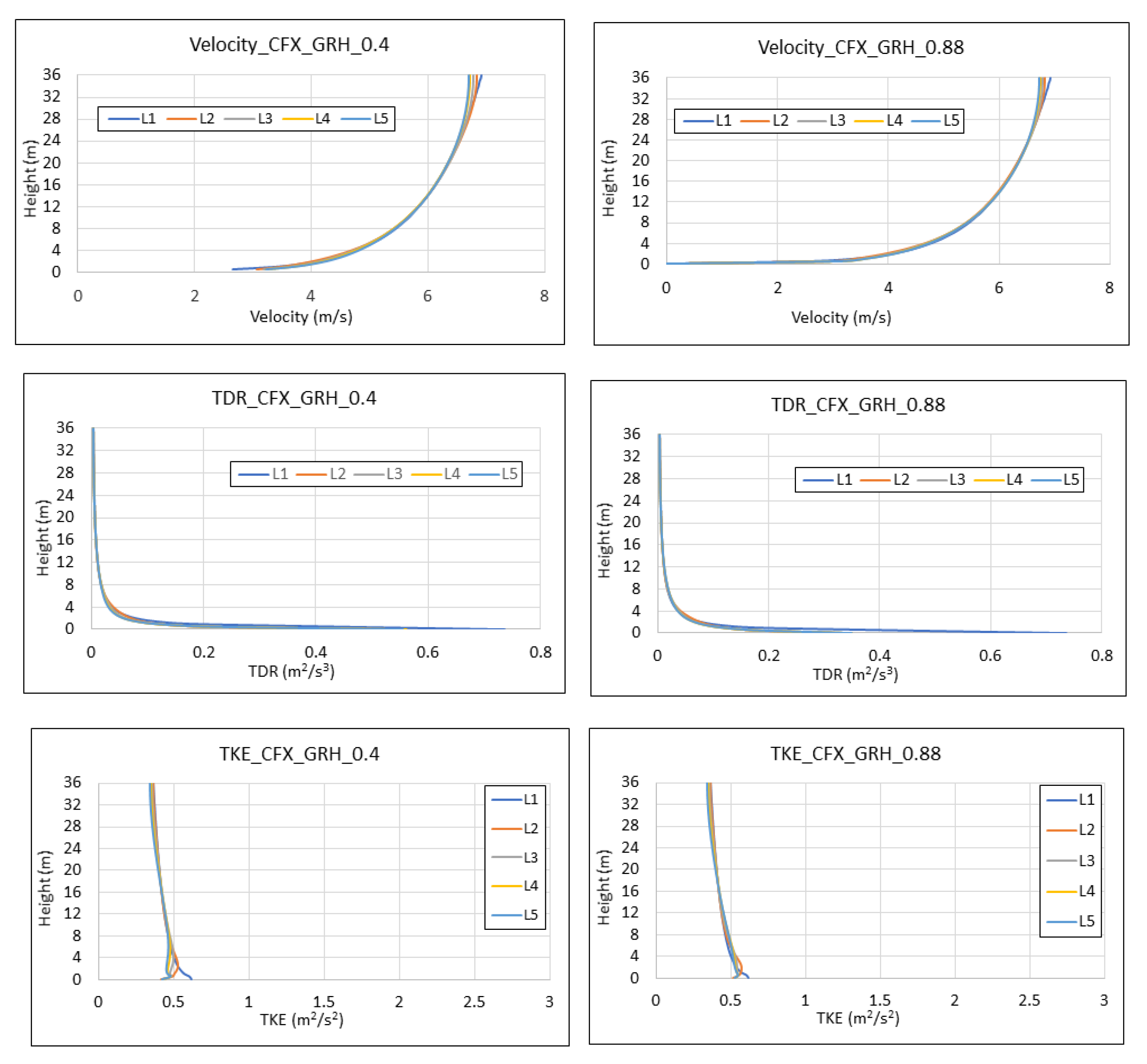
Figure 8 shows the velocity, TKE, and TDR vertical profiles from the two simulations, where visually one may conclude that using the Zs = 0.88 m value appears to result in a better performance. A more quantitative analysis is presented in Figure 9 and Figure 10 using the Mean Absolute Percentage Errors/differences (MAPEs) (Equation (1)) and the Q-value (Equation (2)), as done for Case 1. From Figure 9, we can see that using the Zs = 0.88 m value results in lower variations for the velocity and TKE profiles, with maximum MAPE values reaching 1% and 4%, respectively, whilst, for the TDR profile, the Zs = 0.4 m value results in a value lower (below 6%) than for Zs = 0.88 m (higher than 7%), although the difference is not high.
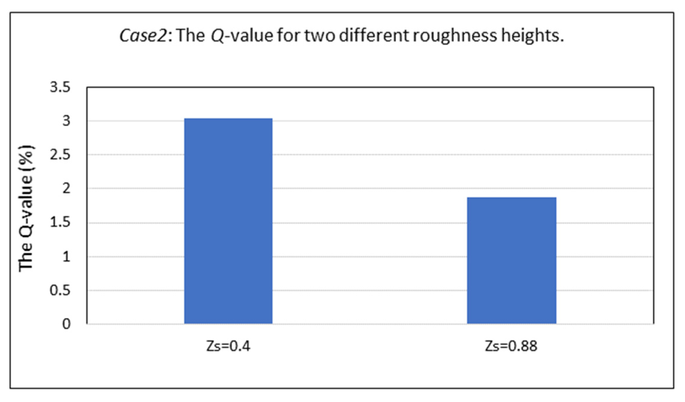
The Q-value for each parameter (velocity, TDR, and TKE) is shown in Figure 10. It is clear from Figure 10 that, for Case 2, the CFX software performs better when the Zs value is set to Zs = 0.88 m, with the average MAPE value over all parameters and all locations being less than 2%, as opposed to 3% when the Zs value is set to Zs = 0.4 m. The difference is very small; however, the value of Zs = 0.88 m for the CFX simulations was subsequently considered for both Cases 2 and 3.
Having established the most preferred Zs value for the CFX software (Zs = 0.88 m), the results for all simulations—for the three software—were then compared and presented in Figure 11 and Figure 12. Figure 11 shows the vertical variation of the profiles for the parameters of interest (velocity, TDR, and TKE), whilst Figure 12 shows the MAPE values (Equation (1)) for each software. Visually, from Figure 11, we see all software retain the HHABL profile within the domain considerably well. Figure 12 shows a more quantitative analysis of our results, with the variations of the MAPE values for each parameter presented.
From Figure 12, the smallest mean variations (MAPE values) for the velocity and TDR profiles seem to be resulting from the STAR-CCM+ software, with mean variations less than 0.6% for the velocity profile and less than 5% for the TDR profile. Fluent and CFX exhibit slightly higher values—up to 1.2% with Fluent for the velocity profile and up to 7% (again Fluent) for the TDR profile. The Fluent application also seems to result in the highest mean variation for TKE, with a mean value of just over 8%, followed by STAR-CCM+, with a mean value just over 6%, whilst the CFX application results in the lowest variations of less than 4%.
As for Case 1, we also estimated the standard deviations (SDs) for the MAPE data presented in Figure 12, as shown in Table 6. For this case, we observe a lowering of the MAPE values for all parameters—compared to Case 1—in all software simulations, with the exception of the Fluent velocity simulations, which show a slight increase (around 3%), as opposed to <1% in Case 1. The lowest MAPE values were obtained with the STAR-CCM+ simulations. As in Case 1, the SDs of the MAPE values were also estimated, and again, as in Case 1, these were of the same order as the MAPE values. For Case 2, the lowest MAPE values are obtained for the velocity parameter, using the STAR-CCM+ software. Correspondingly, the lowest SD values are also observed with the STAR-CCM+ simulation results for the velocity, with typical values of around 1%. The highest MAPE values are obtained for the TDR parameter (between 4 and 7%), with the corresponding highest SDs for the same parameter (~10% using the CFX software). It is important to note that Case 2 uses more realistic inlet conditions for all three parameters (velocity, TDR, and TKE) and appropriate wall functions/boundary conditions for the solid, bottom surface. Thus, it is not surprising that the overall results are improved, and lower MAPE values are observed, as well as lower SDs, with the exception of TDR using the CFX software.

3.3. Case 3

As discussed in [12,19,20], the near-ground streamwise gradients preventing the HHABL profile can be eliminated if the outlet profile of a similar simulation in a longer domain (10,000 m and 5000 m, respectively) is used as the inlet profile of the same domain. However, for limited computational power available, our simulations with Fluent and CFX were run with the original domain length of 126 m (in the x-direction), with the exception of the STAR-CCM+ simulations, which considered a domain of 252 m in length (x-direction). In the Fluent and CFX simulations, the output from Case 2 was considered as the inlet conditions for Case 3. For the STAR-CCM+ simulations, as the domain was already twice as long, the vertical profiles from the locations at x = 157.5 m, x = 189 m, x = 220.5 m, and x = 252 m were considered. The results for all simulations are shown in Figure 13 and Figure 14.
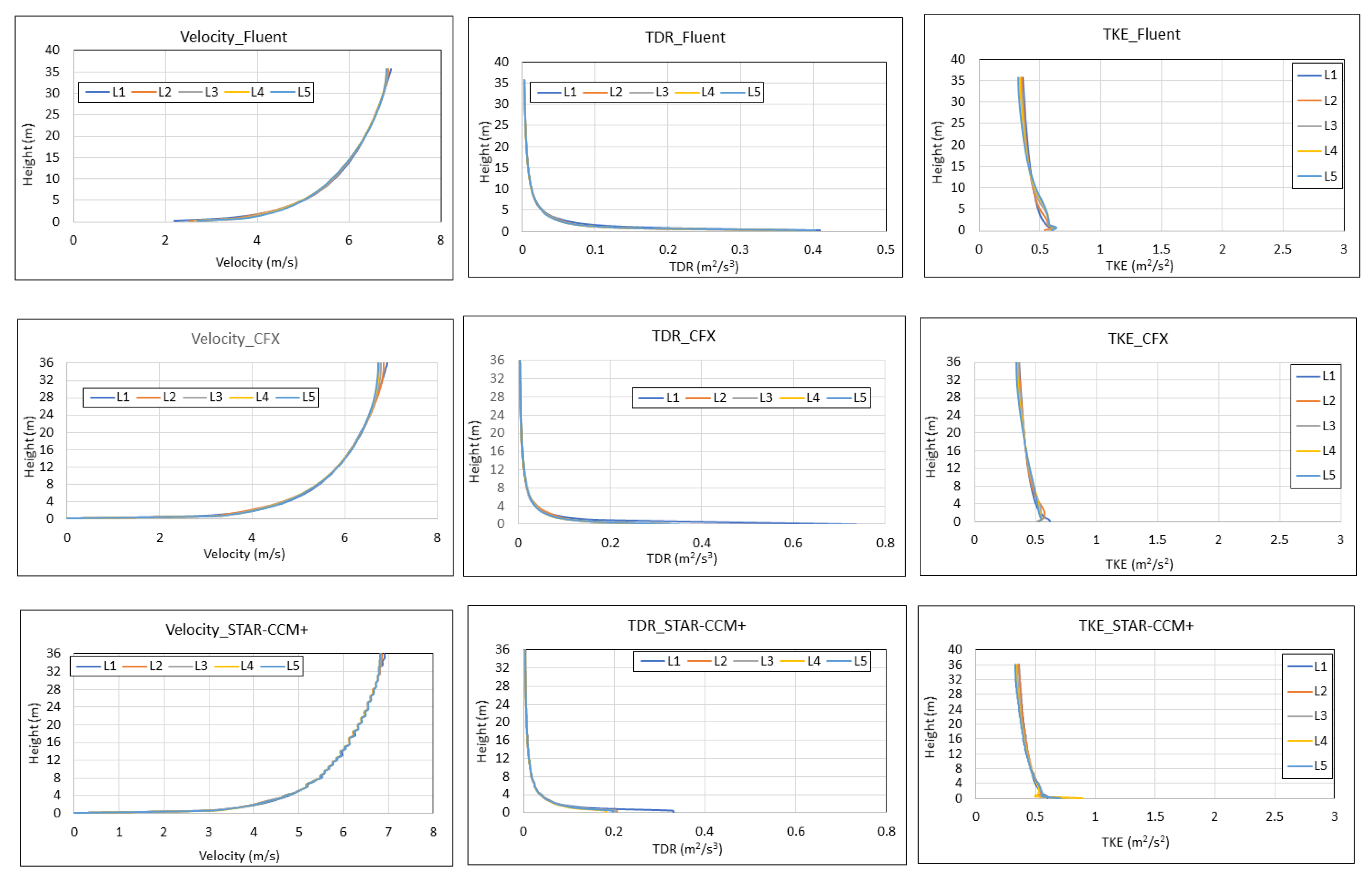
From Figure 13, it can be seen the vertical profiles for the three parameters (u, TKE, and TDR) are well-preserved, with small variations, whilst Figure 14 compares the mean variations for each parameter using the three software.
It is interesting again to see, from Figure 14, that the lowest MAPE values for the velocity (0.25%) and TDR (3%) profiles are obtained from the STAR-CCM+ software (except for the L1 location), followed by Fluent, with mean variations close to 0.3% for the velocity profile and 5.5% for TDR. The CFX software result in 0.4% variations for the velocity profile and 3% for the TDR profile, with the lowest TKE variations (less than 4%) (again, except for the L1 location). STAR-CCM+ results in the highest variation value—close to 7%—followed by the Fluent results reaching 5%.
As for Cases 1 and 2, we also estimated the standard deviations (SDs) of all the MAPE values (Figure 14) for Case 3 (longer 252-m domain), and the results are presented in Table 7. It is interesting to observe a considerable lowering of the MAPE values for all parameters in all software, with the corresponding SDs also being lower now and, again, also of the same order of magnitude as the MAPE values. The lowest MAPE values are obtained for the velocity parameter, with very similar values for all software (<0.5%), with correspondingly low SD values. The highest MAPE values are observed again for the TDR parameter using the CFX software. It is important to note that Case 3 uses as inlet boundary conditions the outlet values of Case 2.

4. Discussion

The work presented in this paper looks at a detailed analysis of the HHABL profile through the variations of three parameters, namely the streamwise velocity (u), the turbulent kinetic energy (TKE), and the turbulent dissipation rate (TDR), through an empty domain. Three different commercial software were implemented—these being the ANSYS Fluent, the ANSYS CFX, and the Siemens STAR-CCM+. The simulation results presented consisted of: (i) graphical plots of the vertical profiles of the parameters of interest (u, TKE, and TDR) in relation to the inlet values (Figure 6, Figure 11 and Figure 13); the mean absolute percentage errors/differences (MAPEs) at the locations downstream the inlet for each parameter in relation to the inlet profiles using the three software (Figure 7, Figure 12 and Figure 14); and the average of all MAPE values over all parameters and all locations for all cases and all three software, resulting in the Q-values, as presented in Figure 15. Three cases were studied—characterized by different inlet conditions—as shown in Table 2, with the more realistic inlet conditions specified in Cases 2 and 3.
Although there has been substantial past work in the literature relating to the HHABL, there is very limited/almost nonexistent detailed analysis in the form presented in this paper, i.e., through the analysis of the mean absolute percentage errors (MAPEs) for the three parameters of interest (u, TDR, and TKE). The closest reference we found that reported percentage errors/differences between inlet conditions and values downstream was in [19], where the average percentage error (APE) was presented at two specific heights only (at 2 m and 20 m) but not the mean values over the whole profile, as presented here. From [19], we noticed their APEs were very high—in some cases, approaching over 50% for TDR—within a computational domain of 10,000 m. In our study, we obtained the average APE over the whole vertical profile of 36 m (averaging over 72 elevations), i.e., our MAPE values, as presented in Table 5, Table 6 and Table 7, together with their SDs. Subsequently, we estimated the average MAPE over all locations—together with the average SDs—as presented again in Table 5, Table 6 and Table 7, and it can be seen from these tables, the average MAPEs over all locations, taking into account the addition of the SDs range: (a) for Case 1: (i) for velocity—between 1.5% to 17%, (ii) for TDR—between 10% and 40%, and (iii) for TKE—between 11% and 17%; (b) for Case 2: (i) for velocity—between 1.5% and 4%, (ii) for TDR—between 10% and 16%, and (iii) for TKE—between 5% and 10%; and (c) for Case 3: (i) for velocity—less than 1%, (ii) for TDR—less than 6%, and for (ii)—less than 7%.
A substantial decrease in the average MAPEs is observed in Cases 2 and 3, relative to Case 1, showing that improved inlet conditions and a longer domain result in improving the HHABL.
It can also be seen that the average MAPE values for all parameters for Case 3 are much lower than the individual APE values reported in [19]; however, for Case 1, the average MAPE value for TDR reaches values similar values to the ones reported in [19], i.e., up to 40% vs. over the 50% noted in [19].
In more detail, looking at Figure 7, Figure 12 and Figure 14 and Table 5, Table 6 and Table 7, our results show the following:
  • Case 1 shows the largest MAPEs amongst the software, with Fluent and STAR-CCM+ exhibiting acceptable HHABL for the velocity and TDR profiles, whilst CFX exhibits the largest MAPEs from the inlet profile, averaging a value over all locations of ~5% for the velocity, with an SD of near 12%, whilst, for the TDR profile, the location-averaged MAPEs are close to 15%, with a corresponding SD of 25% (Table 5). The lowest TDR variations are observed with Ansys Fluent, with a location-averaged MAPE value of 5.6% and a corresponding SD of 4.5%, whilst STAR-CCM+ exhibits slightly higher values of 7.9% and 9.8% (SD values). It is noted that STAR-CCM+ software implements a two-layer k–ε realizable model, where the TDR value in the layer near the wall is estimated using the Wolfstein expression, as opposed to the transport equation. In contrast, the CFX software results in the lowest TKE differences, with a location-averaged MAPE of 5.5% and the lowest SD of nearly 6%, whilst Fluent and STAR-CCM+ exhibit higher location-averaged MAPEs, nearing 12%, but lower corresponding SDs of 3.1% and 4.6%, respectively (Table 5). These higher variations in TKE may not be surprising, as the inlet TKE profile is an unrealistic, constant (with height) profile, although CFX seems to be able to preserve the TKE profile better than Fluent and STAR-CCM+.
  • Case 2 exhibits a good HHABL profile for all three software. For Case 2, the best overall performance for the velocity profiles appears to be with the STAR-CCM+ software, where the location-averaged MAPEs are less than 0.5% and, also, have the lowest SDs (<1%). For the TDR profiles, STAR-CC+ results in the lowest location-averaged MAPE value of 4.22%, with a similar value by the Fluent software, but STAR-CCM+ appears to have a higher SD (7%), as opposed to the ~5% of SD using Fluent. The CFX software results in the slightly higher location-averaged value of the MAPE (5.95%) and the highest corresponding SD (10.1%) (Table 6). It is noted that STAR-CCM+ implements the blended wall function, and a higher resolution mesh is necessary (base cell size of 0.1 m), in combination with a relative velocity of −12 m/s and a roughness length of 0.03 m, as opposed to the roughness height Zs = 0.4 m in Fluent and Zs = 0.88 m in CFX. The differences in the TDR values between STAR-CCM+ and the other two software (ANSYS Fluent and ANSYS CFX) may be again due to the fact that, in STAR-CCM+, a two-layer k–ε realizable model was implemented, in which the TDR value in the layer near the wall was estimated using the Wolfstein expression, as opposed to the transport equation. Although the ANSYS CFX software did not perform as well as the other two software for the velocity and TDR profiles, it seemed to perform better than Fluent and STAR-CCM+ in relation to the TKE, exhibiting the lowest location-averaged values and SDs, as seen in Table 6.
  • Case 3 shows the lowest MAPE values (Table 7), with STAR-CCM+ performing best in preserving the inlet velocity and TDR profiles, with the lowest average (over all locations) MAPE values being less than 0.25% for velocity and less than 2% for TDR, respectively, whilst the CFX software succeeds in preserving the TKE profiles, with the lowest average (over all locations) MAPEs less than 3%.
  • STAR-CCM+ differs from the other two software in its implementation of the blended wall function approach and the estimation of the TDR near the wall using Equation (25), as opposed to the full transport equation (Equation (16)). Results for the TDR predictions from Table 5, Table 6 and Table 7 indicate that, for Case 1, STAR-CCM+ performed better than CFX but worse than Fluent. For Case 2, STAR-CCM+ resulted in the lowest MAPE values (for TDR), compared to Fluent and CFX, indicating perhaps that the blended function approach is a better approach. However, the corresponding SDs with STAR-CCM+ were higher than Fluent. For Case 3, STAR-CCM+ resulted in the lowest MAPE values for TDR and the lowest SDs. The improved simulation results using STAR-CCM+ for Case 3 may be attributed to the blended wall function approach and the two-layer k-e approach, with the implementation of the Wolfstein expression for the estimation of the near-wall TDR values
  • The SDs estimated in all cases for all parameters and all three software are, in most cases, of the same order as the corresponding MAPE values, with Case 3 showing the lowest MAPE values, as well as the lowest SD values, as seen in Table 5, Table 6 and Table 7. The averaged MAPEs and averaged SDs (over all locations) for each parameter are also shown in Table 7, clearly indicating that the lowest values are obtained with Case 3. Highest variations in the averaged MAPEs occur for the TKE in all software, with values ranging from 2% to ~5%, whilst the corresponding SDs are close to 3% for all three software.
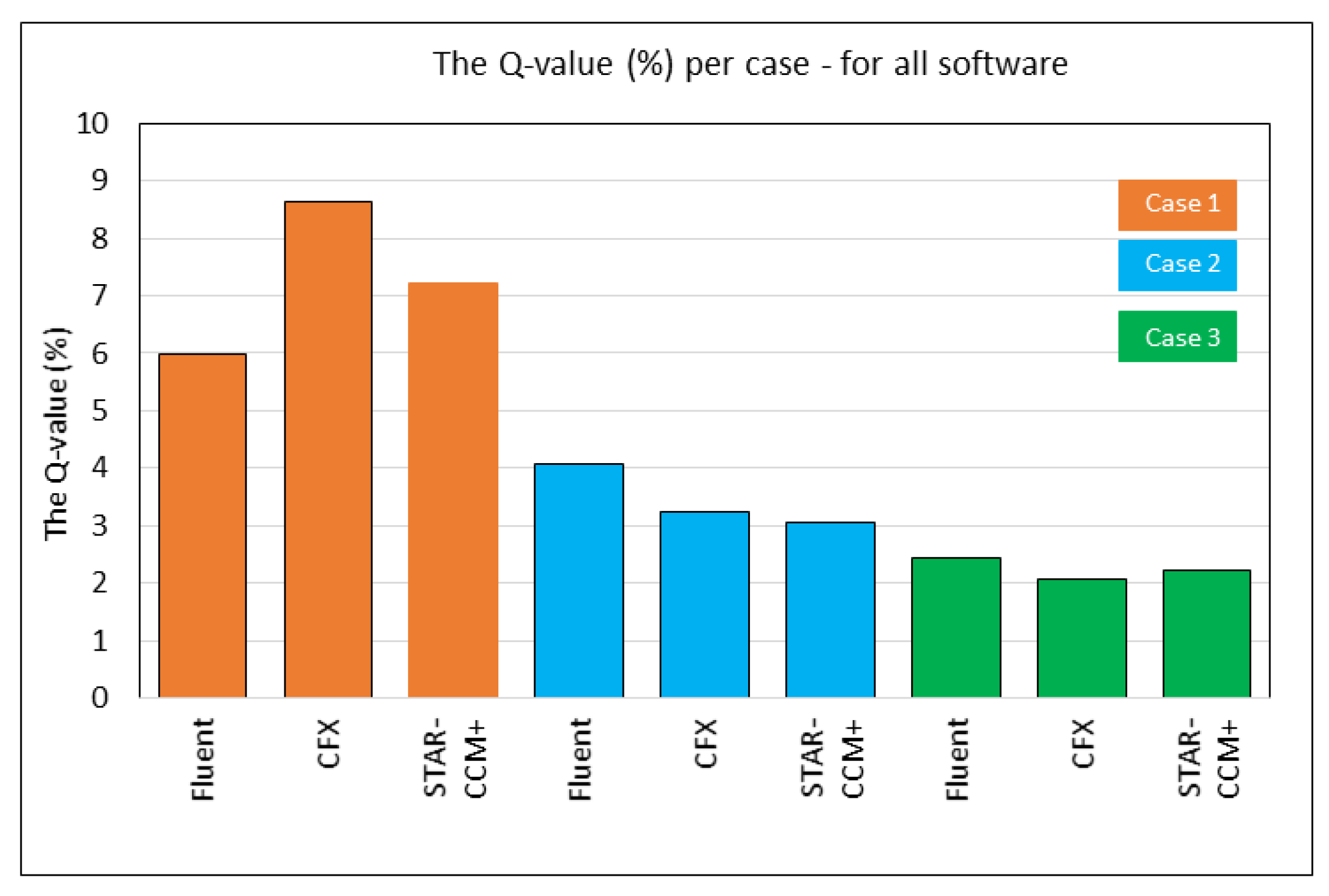
To assess further the quality of the HHABL, in addition to the location-averaged values presented in Table 5, Table 6 and Table 7, the MAPE values were also subsequently averaged over all the parameters to get a “holistic” idea of how each software behaves. This averaging over all locations and over all parameters represents the Q-values (Equation (2)) that were determined for each case using the different software. In addition, the corresponding SDs are also estimated and shown in Table 8. Graphically, the Q-values are shown in Figure 15.
From Table 8 and Figure 15, we observe the following:
For Case 1: Fluent and STAR-CCM+ result in very similar variations (sums of mean variations over all parameters being 6% and 7%, respectively), whilst CFX results in a higher value of 8.63%, with the highest SD of 14.2%. Two possible reasons may be: (i) the fact that CFX software does not provide a realizable k–ε model but allows only the standard k–ε model, and (ii) the wall boundary conditions are slightly different between the three software, with Fluent utilizing the standard wall function, STAR-CCM+ implementing the blended wall function approach, and CFX the scalable wall function. For Case 1, the Fluent application seems to retain the HHABL profile better, with the lowest Q-values and associated SDs (6% and 2.8%, respectively), followed by STAR-CCM+ and then CFX, with CFX also exhibiting the highest SD value of 14.2%.
For Case 2: From Table 8 and Figure 15, we see that, overall, all software perform better than in Case 1, with STAR-CCM+ appearing to have the smallest Q-values (just reaching 3%) and associated SD (3.94%), followed by CFX with a very slightly higher Q-value of 3.24% and a corresponding SD of 4.94%, whilst Fluent results in the largest Q-value of 4% and corresponding SD of 3.44%. These percentage differences are, overall, the same amongst the software, and all three software appear to be behaving in a very similar manner and resulting in a good preservation of the HHABL profile within the domain.
For Case 3: In this case, from both Table 8 and Figure 15, we can see that all three software result in lower Q-values and associated SDs in relation to Case 2, with overall Q-values ranging from 2.06% with the CFX results, followed by STAR-CCM+ with 2.2% and Fluent just over 2.4%. Their corresponding SDs are also of the same order, with STAR-CCM+ resulting in the lowest SD value of 1.5%, whilst Fluent results in an SD of 1.79%.
It is clear that these variations amongst the software are minimal, with all software exhibiting overall Q-values less than 2.5%, with corresponding SD values also less than 2%—hence, showing very similar performances for Case 3. A threshold Q-value of 5% was considered and all three software seemed to perform well based on this threshold—with regards to the preservation of the HHABL profile.
It is interesting to note again that the Q-values obtained are lower than the error values presented in [19]. The differences in the output from the different software for each case may be due to the inlet conditions and length of the domain. We recall that Case 1 consists of an unrealistic TKE inlet profile and results in the higher Q-values and associated SD values for all software. Case 2 has realistic inlet profiles for all parameters (u, TKE, and TDR) and results in Q-values lower than Case 1, as well as lower SD values; however, the computational domain is not very long—only 126 m. Case 3 represents a longer domain (252 m) and results in the lowest Q-values—less than 2.5%—and the lowest SD values, with all software showing very similar values; only a 0.5% difference was amongst the software values, indicating that all three software preserved satisfactorily the HHABL profile, assuming the correct boundary conditions and model parameters are implemented.

5. Conclusions

The outcome of this work indicated that all three software achieve the HHABL profile, with minor differences between them, provided realistic inlet conditions are implemented and the right simulation parameters are chosen (e.g., roughness height). This is obvious in Cases 2 and 3, where differences of less than 2% amongst the software overall mean values (Figure 15) are observed. Case 3 results in the best overall results, with the lowest Q-value, as shown in Figure 15 and Table 8, with all three software yielding very similar values and less than 0.5% difference between the software, confirming the fact that, when the correct boundary conditions and model parameters are implemented, a satisfactory horizontal homogeneity for the ABL can be achieved within the domain.
Possible reasons for the small differences observed between the software may be due to:
  • The varying meshing options chosen in the different software, i.e., the prism-layer option given in STAR-CCM+, as opposed to the uniform/structured mesh in Fluent and CFX. It is noted that higher resolution meshes were considered in both Fluent and CFX but with no visible improvement in the HHABL profile, consistent with the findings of previous research.
  • Slight variations in the expressions for the eddy viscosity models (Equations (5) and (8)).
  • Slight variations in the wall boundary condition functions. As was discussed in Section 2.2.3, slightly different wall functions were implemented in the three software, with the standard wall function in Fluent, the scalable wall function in CFX, and the blended wall function in STAR-CCM+. Similar constants were used in the three functions; however, for example, the scalable wall function implemented in CFX may be a more suitable function than the standard wall function, as it overcomes the inconsistencies/inaccuracies near the wall when higher resolution meshes are used near the wall. STAR-CCM+ implemented the blended wall function, and, in combination with a high-resolution mesh (bases size of 0.1 m) and a relative velocity, it resulted in a good preservation of the profiles for both Cases 2 and 3. When using a structured, uniform mesh with a base cell size of 0.5 m, without a finer resolution near the wall, STAR-CCM+ did not perform as well as the other software.
  • Slight differences in the k ε turbulence model, as the realizable k ε model was implemented in both the Fluent and STAR-CCM+ applications, whilst only the standard k ε model was available in the CFX software.
  • Further works will consider the implementation of the same three software, with the inclusion of a single obstacle within the domain, to assess again the possible differences between the three software for the estimation of turbulence quantities.

Author Contributions

I.A. conceptualized the paper, provided the initial ANYS Fluent simulation model, literature review and material for the paper. He supervised and reviewed the paper during all stages of its progression and managed the collaboration between Applied Science University (ASU), Bahrain, and London South Bank University (LSBU), UK after successfully securing the funding for this research. A.H. wrote the introduction and carried out additional Fluent simulations, as well as the associated statistical analysis and graphical presentation of the results from all three software. E.A. carried out the STAR-CCM+ simulations, together with the associated statistical analysis, as well as undertook the major component of writing, editing, and reviewing of the paper. R.S. carried out the Fluent and CFX simulations, assisted with the writing related to the Fluent and CFX simulations, and managed the project from the LSBU side with ASU. All authors have read and agreed to the published version of the manuscript.

Funding

This research is funded by the Applied Science University (ASU) in Bahrain through an internal competition. It is part of a bigger research project funded by the Applied Science University (ASU), Bahrain in partnership with London South Bank University (LSBU), UK.

Acknowledgments

We are grateful for the reviewers’ comments for their constructive and helpful insights.

Conflicts of Interest

The authors declare no conflict of interest.

References

  1. Blocken, B. Computational Fluid Dynamics for urban physics: Importance, scales, possibilities, limitations and ten tips and tricks towards accurate and reliable simulations. Build. Environ. 2015, 91, 219–245. [Google Scholar] [CrossRef] [Green Version]
  2. Lateb, M.; Meroney, R.; Yataghene, M.; Fellouah, H.; Saleh, F.; Boufadel, M. On the use of numerical modelling for near-field pollutant dispersion in urban environments—A review. Environ. Pollut. 2016, 208, 271–283. [Google Scholar] [CrossRef] [PubMed] [Green Version]
  3. Yan, B.; Li, Q.; He, Y.; Chan, P. RANS simulation of neutral atmospheric boundary layer flows over complex terrain by proper imposition of boundary conditions and modification on the k-ε model. Environ. Fluid Mech. 2016, 16, 1–23. [Google Scholar] [CrossRef]
  4. Chang, C.-Y.; Schmidt, J.; Dörenkämper, M.; Stoevesandt, B. A consistent steady state CFD simulation method for stratified atmospheric boundary layer flows. J. Wind Eng. Ind. Aerodyn. 2018, 172, 55–67. [Google Scholar] [CrossRef]
  5. Abohela, I.; Hamza, N.; Dudek, S. Effect of roof shape, wind direction, building height and urban configuration on the energy yield and positioning of roof mounted wind turbines. Renew. Energy 2013, 1106–1118. [Google Scholar] [CrossRef]
  6. van Hooff, T.; Blocken, B.; Tominaga, Y. On the accuracy of CFD simulations of cross-ventilation flows for a generic isolated building: Comparison of RANS, LES and experiments. Build. Environ. 2017, 114, 148–165. [Google Scholar] [CrossRef]
  7. Blocken, B.; Stathopoulos, T.; van Beeck, J.P.A.J. Pedestrian-level wind conditions around buildings: Review of wind-tunnel and CFD techniques and their accuracy for wind comfort assessment. Build. Environ. 2016, 100, 50–81. [Google Scholar] [CrossRef]
  8. Toparlar, Y.; Blocken, B.; Vos, P.; Van Heijst, G.; Janssen, W.; van Hooff, T.; Timmermans, H. CFD simulation and validation of urban microclimate: A case study for Bergpolder Zuid, Rotterdam. Build. Environ. 2015, 83, 79–90. [Google Scholar] [CrossRef] [Green Version]
  9. Guo, W.; Liu, X.; Yuan, X. Study on Natural Ventilation Design Optimization Based on CFD Simulation for Green Buildings. Procedia Eng. 2015, 121, 573–581. [Google Scholar] [CrossRef] [Green Version]
  10. Abohela, I. On the horizontal homogeneity of the Atmospheric Boundary Layer in CFD simulations. Appl. Math. Inf. Sci. 2018, 12, 825–829. [Google Scholar] [CrossRef]
  11. Hu, C.-H. Proposed Guidelines of Using CFD and the Validity of the CFD Models in the Numerical Simulations of Wind Environments around Buildings. Ph.D. Thesis, Heriot-Watt University, Edinburgh, UK, 2013. [Google Scholar]
  12. Hargreaves, D.M.; Wright, N.G. On the use of the k-[epsilon] model in commercial CFD software to model the neutral atmospheric boundary layer. J. Wind Eng. Ind. Aerodyn. 2007, 95, 355–369. [Google Scholar] [CrossRef]
  13. Cai, X.; Huo, Q.; Kang, L.; Song, Y. Equilibrium atmospheric boundary-layer flow: Computational fluid dynamics simulation with balanced forces. Bound. Layer Meteorol. 2014, 152, 349–366. [Google Scholar] [CrossRef]
  14. Aly, A.M. Atmospheric boundary-layer simulation for the built environment: Past, present and future. Build. Environ. 2014, 75, 206–221. [Google Scholar] [CrossRef]
  15. Richards, P.J.; Younis, B.A. Comments on “Prediction of the wind-generated pressure distribution around buildings” by E.H. Mathews. J. Wind Eng. Ind. Aerodyn. 1990, 34, 107–110. [Google Scholar] [CrossRef]
  16. O’Sullivan, J.; Archer, R.; Flay, R. Consistent boundary conditions for flows within the atmospheric boundary layer. J. Wind Eng. Ind. Aerodyn. 2011, 99, 65–77. [Google Scholar] [CrossRef]
  17. Mathews, E.H. Prediction of the wind-generated pressure distribution around buildings. J. Wind Eng. Ind. Aerodyn. 1987, 25, 219–228. [Google Scholar] [CrossRef]
  18. Zhang, C.X. Numerical prediction of turbulent recirculating flows with a k-e model. J. Wind Eng. Ind. Aerodyn. 1994, 51, 177–201. [Google Scholar] [CrossRef]
  19. Blocken, B.; Stathopoulos, T.; Carmeliet, J. CFD simulation of the atmospheric boundary layer: Wall function problems. Atmos. Environ. 2007, 41, 238–252. [Google Scholar] [CrossRef]
  20. Blocken, B.; Carmeliet, J.; Stathopoulos, T. CFD evaluation of wind speed conditions in passages between parallel buildings—Effect of wall-function roughness modifications for the atmospheric boundary layer flow. J. Wind Eng. Ind. Aerodyn. 2007, 95, 941–962. [Google Scholar] [CrossRef]
  21. Launder, B.E.; Spalding, D.B. The numerical computation of turbulent flows. Comput. Methods Appl. Mech. Eng. 1974, 3, 269–289. [Google Scholar] [CrossRef]
  22. Quinn, A.D.; Wilson, M.; Reynolds, A.M.; Couling, S.B.; Hoxey, R.P. Modelling the dispersion of aerial pollutants from agricultural buildings—An evaluation of computational fluid dynamics (CFD). Comput. Electron. Agric. 2001, 30, 219–235. [Google Scholar] [CrossRef]
  23. Riddle, A.; Carruthers, D.; Sharpe, A.; McHugh, C.; Stocker, J. Comparisons between FLUENT and ADMS for atmospheric dispersion modelling. Atmos. Environ. 2007, 38, 1029–1038. [Google Scholar] [CrossRef]
  24. Miles, S.; Westbury, P. Practical tools for wind engineering in the built environment. QNET-CFD Netw. Newsl. 2003, 2, 11–14. [Google Scholar]
  25. Franke, J.; Hirsch, C.; Jensen, A.G.; Krüs, H.W.; Schatzmann, M.; Westbury, P.S.; Miles, S.D.; Wisse, J.A.; Wright, N.G. Recommendations on the use of CFD in wind engineering. In Proceedings of the International Conference on Urban Wind Engineering and Building Aerodynamics, Sint-Genesius-Rode, Belgium, 5–7 May 2004. [Google Scholar]
  26. Franke, J.; Frank, W. Numerical simulation of the flow across an asymmetric street intersection. In Proceedings of the 4EACWE, Prague, Czech Republic, 11–15 July 2005. [Google Scholar]
  27. Blocken, B.; Carmeliet, J. The influence of the wind-blocking effect by a building on its wind-driven rain exposure. J. Wind Eng. Ind. Aerodyn. 2006, 94, 101–127. [Google Scholar] [CrossRef]
  28. Richards, P.; Norris, S. Appropriate boundary conditions for a pressure driven boundary layer. J. Wind Eng. Ind. Aerodyn. 2015, 142, 43–52. [Google Scholar] [CrossRef]
  29. Yang, Y.; Gu, M.; Chen, S.; Jin, X. New inflow boundary conditions for modelling the neutral equilibrium atmospheric boundary layer in computational wind engineering. J. Wind Eng. Ind. Aerodyn. 2009, 97, 88–95. [Google Scholar] [CrossRef]
  30. Commercial CFD ANSYS Fluent User Manual R2; Fluent R2; 2020. Available online: https://ansyshelp.ansys.com/account/secured?returnurl=/Views/Secured/prod_page.html?pn=Fluent&lang=en (accessed on 31 May 2020).
  31. Commercial CFD ANSYS CFX User Manual R2; CFX R2; 2020. Available online: https://ansyshelp.ansys.com/account/secured?returnurl=/Views/Secured/prod_page.html?pn=CFX&lang=en (accessed on 31 May 2020).
  32. Commercial Siemens STAR-CCM+ Software Manual. Available online: https://www.plm.automation.siemens.com/global/en/products/simcenter/STAR-CCM.html (accessed on 30 November 2019).
  33. Solari, G. Wind Science and Engineering. In Origins, Developments, Fundamentals and Advancements; Springer: Berlin/Heidelberg, Germany, 2019; ISBN 978-3-030-18814-6. [Google Scholar]
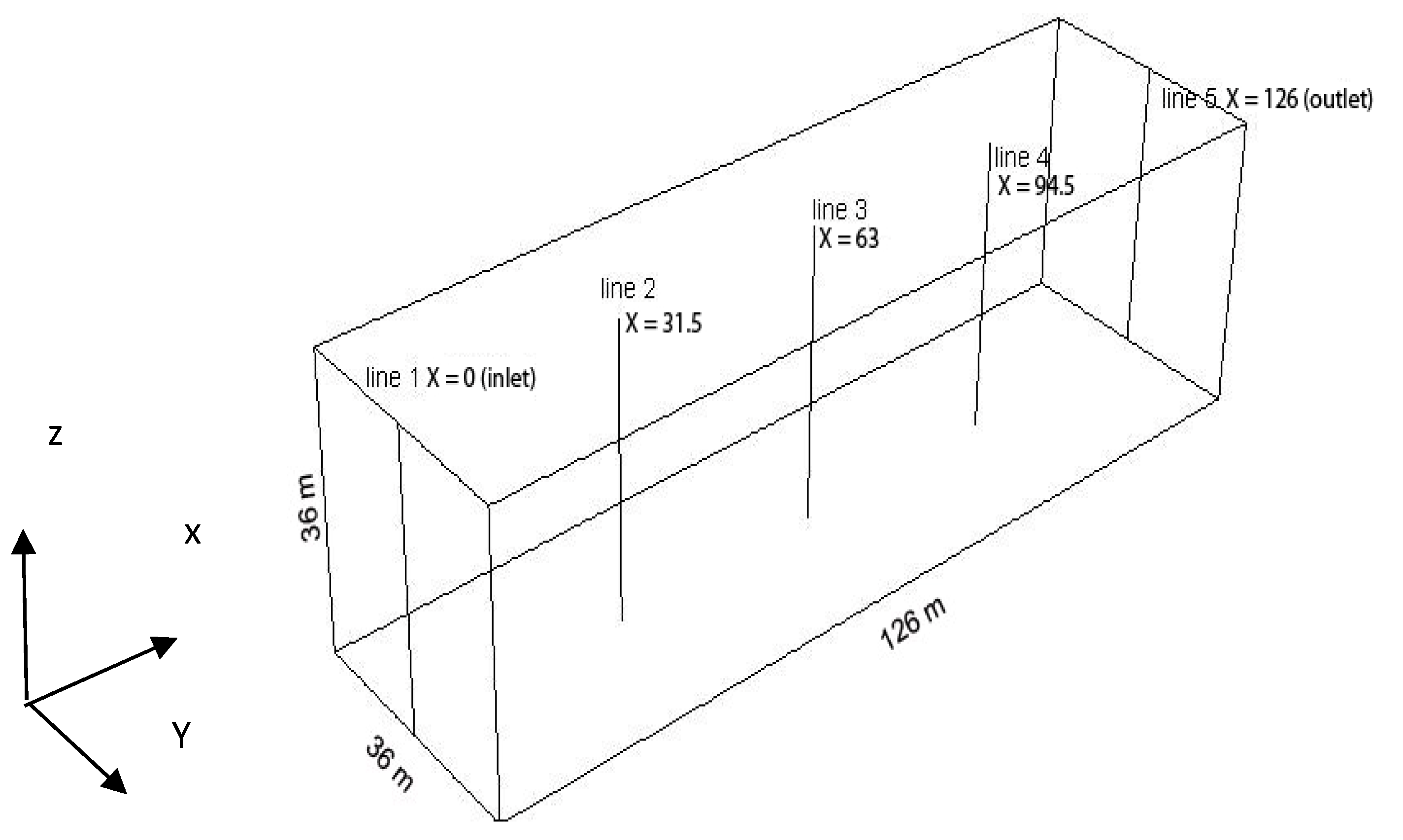
Figure 1. Computational domain dimensions and coordinates of locations L1 (inlet), L2, L3, L4, and L5 (outlet) where the vertical profiles of the streamwise velocity (u) profile and turbulent kinetic energy (TKE) (k) and turbulent dissipation rate (TDR) (ε) profiles were observed. The y-coordinate of all profiles is y =18 m.
Atmosphere 11 01138 g001
Figure 2. The computational domain meshed using equidistant structured mesh in both the Fluent and CFX simulations: (a) the full 3D computational domain and (b) a horizontal (x-y) plane with the computational, structured, hexahedral mesh.
Atmosphere 11 01138 g002
Figure 3. The computational domain meshed using a trimmed (hexahedral elements) mesh. The domain is 252-m-long, resulting in approximately 2,612,736 cells.
Atmosphere 11 01138 g003
Figure 4. The computational domain meshed using the trimmed mostly hexahedral cells with a prism-layer option. The total prism layer thickness is set to 14 m from the wall, whilst the base cell size is 0.1m. The maximum surface cell size is set to 2 m, with the overall number of cells being ~8,000,000 cells.
Atmosphere 11 01138 g004
Figure 5. The inlet boundary conditions for Cases 1 and 2, as per Table 2. For Case 3, the inlet velocity, turbulent kinetic energy, and dissipation rate profiles were based on the outlet values of Case 2.
Atmosphere 11 01138 g005
Figure 6. Case 1: Comparison of the vertical profiles of the streamwise velocity u, turbulent kinetic energy (TKE), and turbulent dissipation rate (TDR) with each software.
Atmosphere 11 01138 g006
Figure 7. Case 1: Comparison of the Mean vertical variations of the Absolute Percentage Error/differences (MAPEs) (based on the results of Figure 6) for each of the parameters (u, TKE (turbulent kinetic energy), and TDR (turbulent dissipation rate) with each software: (i) Fluent and (ii) Star-CCM+ implement the realizable k–ε model, whilst (iii) CFX implements the standard k–ε model.
Atmosphere 11 01138 g007
Figure 8. Case 2: Effect of ground roughness height Zs on: turbulent streamwise velocity, u; turbulent kinetic energy (TKE); and turbulent dissipation rate (ε) using the CFX software. Left column plots is based on Zs = 0.4 m. Right column of plots is based on Zs = 0.88 m.
Atmosphere 11 01138 g008
Figure 9. Case 2: CFX HHABL profile assessment for different ground roughness height Zs: effect of Zs on the Mean Absolute Percentage Errors/differences (MAPE) at each location (relative to the inlet values) for each parameter using the different software.
Atmosphere 11 01138 g009
Figure 10. Case 2: Comparison of the Q-value (Equation (2)), i.e., of the average MAPEs over all parameters and over all locations for the CFX simulations using two different values of the roughness parameter Zs. The two values are Zs = 0.4 m and Zs = 0.88 m. Best results were obtained with Zs = 0.88 m.
Atmosphere 11 01138 g010
Figure 11. Case 2: Comparison of the vertical profiles at the 5 different locations for the streamwise velocity (u), TKE, (k), and turbulent dissipation rate, TDR, (ε) for each software.
Atmosphere 11 01138 g011
Figure 12. Case 2: Comparison of the mean vertical variations of the absolute percentage error/differences (MAPEs) for each parameter (u, TKE, and TDR) using the three software.
Atmosphere 11 01138 g012
Figure 13. Case 3: Comparison of the vertical profiles at the 5 different locations for the streamwise velocity u, turbulent kinetic energy (TKE), and turbulent dissipation rate (TDR) using the three software.
Atmosphere 11 01138 g013
Figure 14. Case 3: Comparison of the mean vertical variations of the absolute percentage errors/differences (MAPEs) for each parameter (u, TKE, and TDR) using the three software.
Atmosphere 11 01138 g014
Figure 15. Comparison of the Q-values (%) (Equation (2)) per case for each software. Case 1 results in the highest values, whilst Case 3 results in the lowest values (<2.5%) with all software showing very similar values (<0.5%) difference between the software.
Atmosphere 11 01138 g015
Table 1. Model Parameters in the Three Software.
Turbulence ModelCases σ k σ ε C ε 1 C ε 2 C μ   Roughness   Length   z 0   ( m ) Roughness Height (m)
Zs
Fluent
Realizable k ε
1, 2, 311.21.44Same as
C2 = 1.9
As per Equation (6)0.030.4
CFX
Standard
k ε
111.21.441.990.090.030.4
211.21.441.920.090.03(i) 0.4 and
(ii) 0.88
311.21.441.920.090.030.88
STAR-CCM+
Realizable   k ε
1, 2, 311.21.441.920.090.03Relative velocity is used instead
Table 2. Inlet Boundary Conditions for the Three Simulation Cases in all Three Software.
Case No.Inlet Profile
(m/s)
Turbulent Kinetic Energy (m2/s2)Turbulent Dissipation Rate ε (m2/s3)
1 u = u κ ln ( z + z 0 z 0 ) u = 0.68   m / s z 0 = 0.03   m k = ( u ) 2 C μ = 1.54133 u = 0.68   m / s ;   C μ = 0.09 ε = u 3 K ( z + z 0 ) u = 0.68   m / s z 0 = 0.03   m
2 u = u κ ln ( z + z 0 z 0 ) u = 0.41   m / s z 0 = 0.03   m k = ( u ) 2 C μ [ C 1 ln ( z + z 0 z 0 ) + C 2 ] u = 0.41   m / s ; C μ = 0.09 ;
z 0 = 0.03   m
ε = u 3 K ( z + z 0 ) [ [ C 1 ln ( z + z 0 z 0 ) + C 2 ] ] u = 0.41   m / s ;   C μ = 0.09 ;
z 0 = 0.03   m
3Output from
Case 2 is used as Inlet for Case 3.
Output from
Case 2 is used as
Inlet for Case 3
Output from
Case 2 is used as
Inlet for Case 3
Table 3. Nondimensional Parameters.
VariableNondimensional Parameter
Wall distance y y + = y ρ u μ
Wall tangential velocity component u of the velocity vector u + = u u
Turbulent eddy viscosity μ t μ t + = μ t μ
Turbulent kinetic energy k k + = k u 2
Turbulent dissipation rate ε ε + = ε μ ρ u 4
Table 4. Wall Boundary Conditions for Each Case Using the Different Software.
Case 1Case 2Case 3
FluentShear wall stress
τ w = ρ u 2 = 0.58 Pa
u + = 1 κ ln ( y + ) + B B u + = 1 κ ln ( y + ) + B B
CFXShear wall stress τ w = ρ u 2 =   0.58 Pa u + = 1 κ ln ( y + ) + C u + = 1 κ ln ( y + ) + C
STAR-CCM+Blended wall function with a Relative velocity of −12 m/sBlended wall function with a Relative velocity of −12 m/sBlended wall function with a Relative velocity of −12 m/s
Table 5. Case 1. CFD: Computational fluid Dynamics, TDR: Turbulent Dissipation Rate, TKE: Turbulent Kinetic Energy, and MAPE: Mean Absolute Percentage Error.
CFD ParameterSoftwareStatistical
Parameters (%)
LocationAverage
Over all Locations (%)
L2-L1L3-L1L4-L1L5-L1
VelocityFluentMAPE0.380.580.750.900.7
SD0.730.780.750.880.8
CFXMAPE2.514.526.237.565.2
SD7.4711.1013.3014.8311.7
STAR-CCM+MAPE0.951.241.331.341.2
SD2.743.213.163.033.0
TDRFluentMAPE2.524.126.659.175.6
SD4.414.934.694.084.5
CFXMAPE7.9512.7917.4822.4615.2
SD20.0524.6727.3428.6825.2
STAR-CCM+MAPE3.536.169.2412.677.9
SD7.319.2410.8411.669.8
TKEFluentMAPE5.199.6114.0217.9111.7
SD1.752.623.584.513.1
CFXMAPE2.604.676.238.445.5
SD4.465.576.466.825.8
STAR-CMM+MAPE4.8310.2715.3719.7012.5
SD3.494.195.045.494.6
Table 6. Case 2.
Table 6. Case 2.
CFD ParameterSoftwareStatistical
Parameters (%)
LocationAverage
Over All Locations (%)
L2-L1L3-L1L4-L1L5-L1
VelocityFluentMAPE0.590.871.071.240.9
SD2.082.703.013.212.75
CFXMAPE0.760.880.981.000.91
SD1.802.262.472.392.23
STAR-CCM+MAPE0.440.440.510.480.47
SD0.760.711.150.880.88
TDRFluentMAPE3.745.196.337.375.67
SD5.304.984.574.564.85
CFXMAPE4.735.896.476.715.95
SD10.2810.2410.049.8010.1
STAR-CCM+MAPE3.264.024.734.884.22
SD6.716.588.006.787.01
TKEFluentMAPE2.604.896.748.155.6
SD1.712.523.123.592.73
CFXMAPE1.642.513.293.972.85
SD2.932.492.242.252.48
STAR-CMM+MAPE2.323.705.486.444.48
SD2.753.295.983.583.9
Table 7. Case 3.
Table 7. Case 3.
CFD ParameterSoftwareStatistical
Parameter
LocationAverage
Over All Locations
L2-L1L3-L1L4-L1L5-L1
VelocityFluentMAPE0.110.210.270.320.23
SD0.130.250.330.380.27
CFXMAPE0.370.340.360.410.37
SD0.680.280.350.300.40
STAR-CCM+MAPE0.200.140.170.260.19
SD0.440.090.120.240.22
TDRFluentMAPE1.553.014.345.503.6
SD1.022.033.054.032.53
CFXMAPE2.572.822.943.122.86
SD3.621.641.622.762.41
STAR-CCM+MAPE1.451.282.103.101.98
SD2.011.021.562.321.73
TKEFluentMAPE1.562.954.165.203.47
SD1.062.083.074.022.56
CFXMAPE2.012.673.243.852.94
SD1.921.362.103.262.16
STAR-CMM+MAPE2.483.555.216.724.49
SD1.311.962.983.922.54
Table 8. Q-Values with their Corresponding SDs.
Case NoSoftwareQ-ValueQ-SD Value
Case 1ANSYS Fluent6.002.80
ANSYS CFX8.6314.23
Siemens STAR-CCM+7.205.80
Case 2ANSYS Fluent4.063.44
ANSYS CFX3.244.94
Siemens STAR-CCM+3.063.93
Case 3ANSYS Fluent2.431.79
ANSYS CFX2.061.66
Siemens STAR-CCM+2.221.50
Publisher’s Note: MDPI stays neutral with regard to jurisdictional claims in published maps and institutional affiliations.