Determining the Impact of Wildland Fires on Ground Level Ambient Ozone Levels in California


Abstract
1. Introduction
2. Experiments
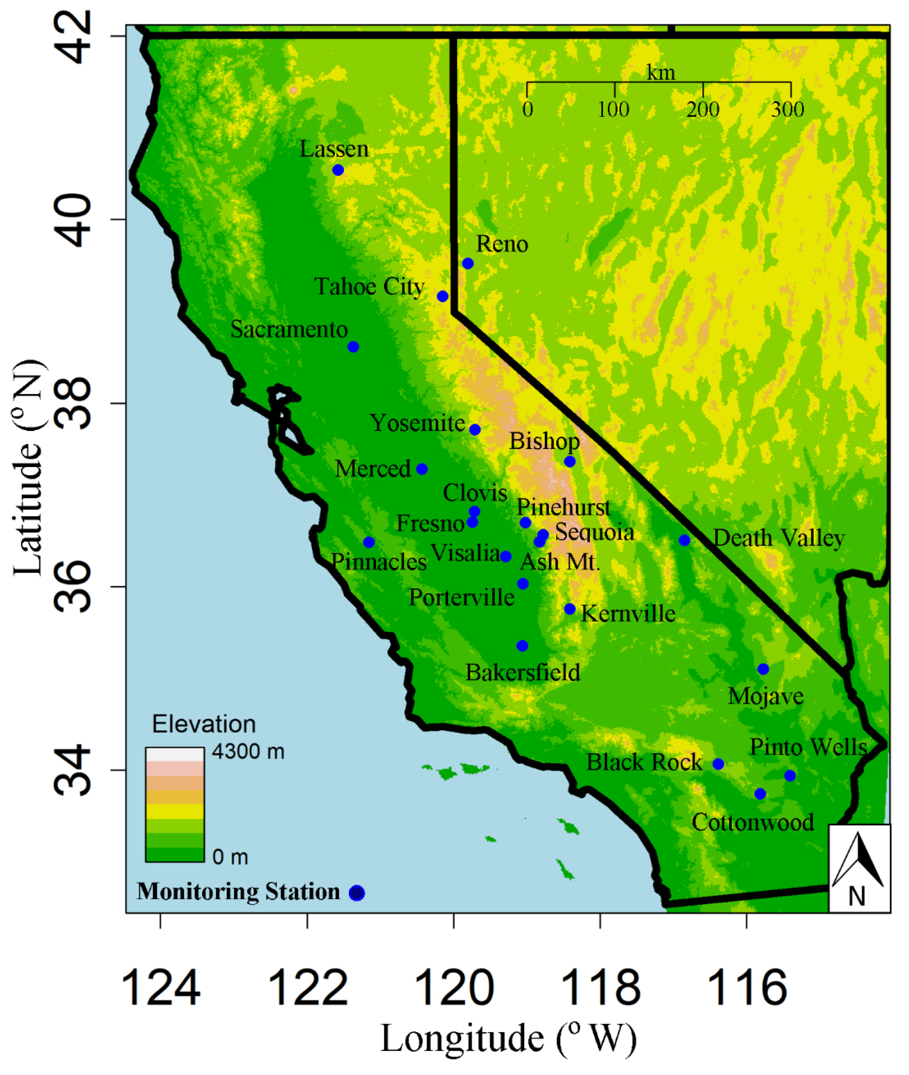
2.1. Study Area
2.2. Ozone and Weather Data
2.3. HMS Data
2.4. Wildland Fire
2.5. Statistical Models
r = 0 otherwise
- (1)
- None—no HMS smoke above site at hour i, day j, year k
- (2)
- Low—Low level of HMS smoke at the hour i, day j, year k
- (3)
- Mid—Medium level of HMS smoke at the hour i, day j, year k
- (4)
- (U Hi, R Hi, B Hi)—High level of HMS smoke at hour i, day j, year k at urban, rural or base sites, respectively
- (5)
- NSFN—Fire within 10 km of the site but no HMS smoke above the site at hour i, day j, year k
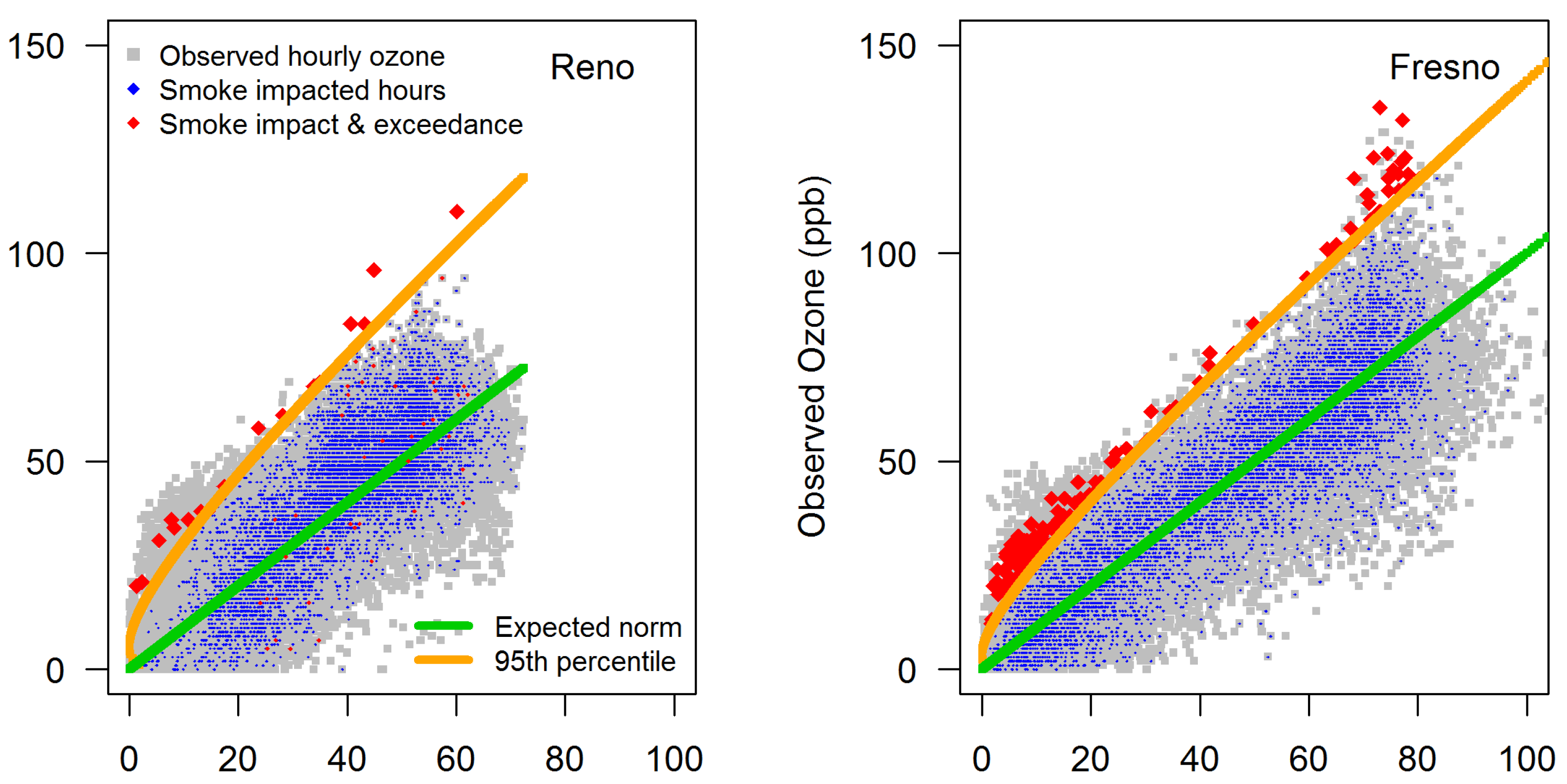
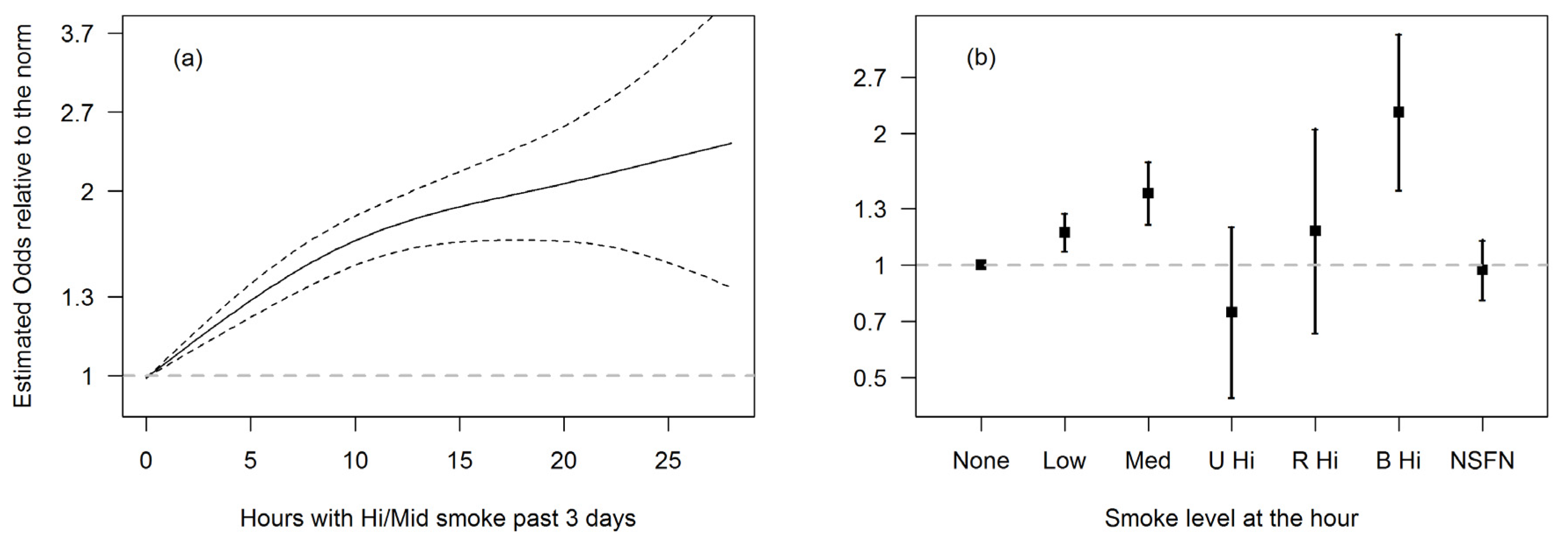
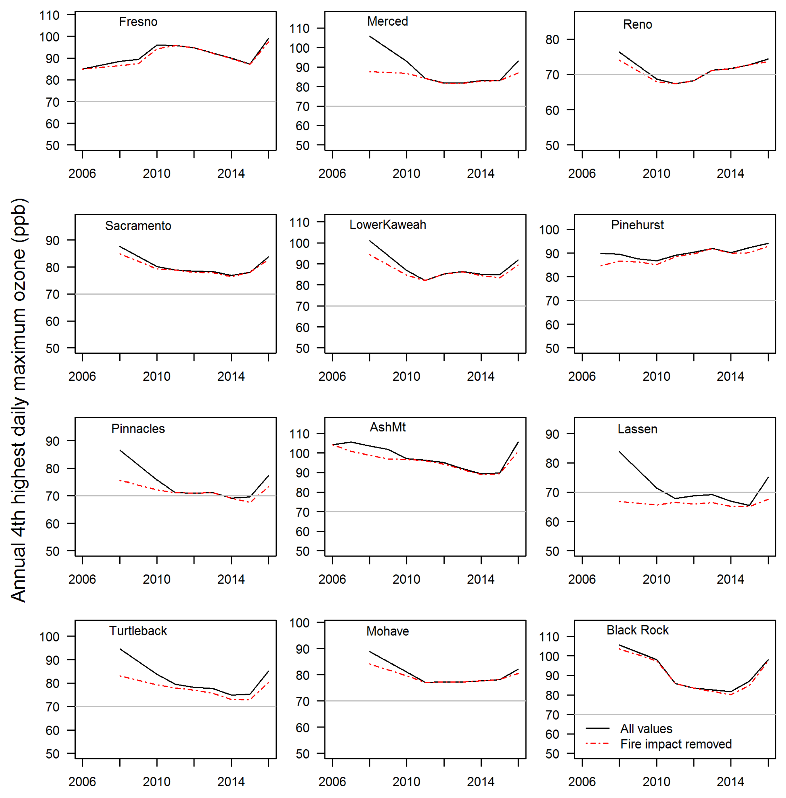
3. Results
Identifying Exceptional Events
4. Discussion and Conclusions
Author Contributions
Funding
Acknowledgments
Conflicts of Interest
References
- Cisneros, R.; Schweizer, D.; Tarnay, L.; Navarro, K.; Veloz, D.; Procter, C.T. Climate Change, Forest Fires, and Health in California. In Springer Climate; Springer International Publishing: Manhattan, NY, USA, 2018; pp. 99–130. [Google Scholar]
- Steel, Z.L.; Safford, H.D.; Viers, J.H. The Fire Frequency-Severity Relationship and the Legacy of Fire Suppression in California Forests. Ecosphere 2015, 6, 8. [Google Scholar] [CrossRef]
- Boisramé, G.F.S.; Thompson, S.; Collins, B.; Stephens, S. Managed Wildfire Effects on Forest Resilience and Water in the Sierra Nevada. Ecosystems 2016, 20, 717–732. [Google Scholar] [CrossRef]
- Van Mantgem, P.J.; Caprio, A.C.; Stephenson, N.L.; Das, A.J. Does Prescribed Fire Promote Resistance to Drought in Low Elevation Forests of the Sierra Nevada, California, USA? Fire Ecol. 2016, 12, 13–25. [Google Scholar] [CrossRef]
- Adams, M.A. Mega-Fires, Tipping Points and Ecosystem Services: Managing Forests and Woodlands in an Uncertain Future. For. Ecol. Manag. 2013, 294, 250–261. [Google Scholar] [CrossRef]
- McMeeking, G.R.; Kreidenweis, S.M.; Lunden, M.; Carrillo, J.; Carrico, C.M.; Lee, T.; Herckes, P.; Engling, G.; Day, D.E.; Hand, J.; et al. Smoke-Impacted Regional Haze in California During the Summer of 2002. Agric. For. Meteorol. 2006, 137, 25–42. [Google Scholar] [CrossRef]
- Kochi, I.; Donovan, G.H.; Champ, P.A.; Loomis, J.B. The Economic Cost of Adverse Health Effects from Wildfire-Smoke Exposure: A Review. Int. J. Wildland Fire 2010, 19, 803–817. [Google Scholar] [CrossRef]
- Kollanus, V.; Prank, M.; Gens, A.; Soares, J.; Vira, J.; Kukkonen, J.; Sofiev, M.; Salonen, R.O.; Lanki, T. Mortality due to Vegetation Fire–Originated PM 2.5 Exposure in Europe—Assessment for the Years 2005 and 2008. Environ. Health Perspect. 2017, 125, 30–37. [Google Scholar] [CrossRef] [PubMed]
- Rappold, A.G.; Reyes, J.; Pouliot, G.; Cascio, W.E.; Diaz-Sanchez, D. Community Vulnerability to Health Impacts of Wildland Fire Smoke Exposure. Environ. Sci. Technol. 2017, 51, 6674–6682. [Google Scholar] [CrossRef] [PubMed]
- Schweizer, D.; Cisneros, R.; Traina, S.; Ghezzehei, T.A.; Shaw, G.D. Using National Ambient Air Quality Standards for Fine Particulate Matter to Assess Regional Wildland Fire Smoke and Air Quality Management. J. Environ. Manag. 2017, 201, 345–356. [Google Scholar] [CrossRef] [PubMed]
- Schweizer, D.; Cisneros, R. Wildland Fire Management and Air Quality in the Southern Sierra Nevada: Using the Lion Fire as a Case Study with a Multi-Year Perspective on PM2.5 Impacts and Fire Policy. J. Environ. Manag. 2014, 144, 265–278. [Google Scholar] [CrossRef]
- CAA. Clean Air Act-As Amended Through P.L. 108-201. 42 U.S.C. §7401; US Government Printing Office: Washington, DC, USA, 2004; pp. 16–17. [Google Scholar]
- California Air Resources. California Code of Regulations, Title 17, 17 CCR § 80100; California Air Resources: Sacramento, CA, USA, 2003. [Google Scholar]
- EER. Part II Environmental Protection Agency 40 CFR Parts 50 and 51 Treatment of Data Influenced by Exceptional Events, Final Rule. Fed. Regist. 2016, 81, 68216–68282. [Google Scholar]
- Gong, X.; Kaulfus, A.; Nair, U.; Jaffe, D.A. Quantifying O3Impacts in Urban Areas Due to Wildfires Using a Generalized Additive Model. Environ. Sci. Technol. 2017, 51, 13216–13223. [Google Scholar] [CrossRef] [PubMed]
- Brey, S.J.; Fischer, E.V. Smoke in the City: How Often and Where Does Smoke Impact Summertime Ozone in the United States? Environ. Sci. Technol. 2016, 50, 1288–1294. [Google Scholar] [CrossRef]
- Jaffe, D.A.; Wigder, N.; Downey, N.; Pfister, G.; Boynard, A.; Reid, S.B. Impact of Wildfires on Ozone Exceptional Events in the Western U.S. Environ. Sci. Technol. 2013, 47, 11065–11072. [Google Scholar] [CrossRef] [PubMed]
- Hoff, R.M.; Christopher, S.A. Remote Sensing of Particulate Pollution from Space: Have We Reached the Promised Land? J. Air Waste Manag. Assoc. 2009, 59, 645–675. [Google Scholar] [CrossRef]
- Toth, T.D.; Zhang, J.; Campbell, J.R.; Hyer, E.J.; Reid, J.S.; Shi, Y.; Westphal, D.L. Impact of Data Quality and Surface-to-Column Representativeness on the PM2.5/Satellite AOD Relationship for the Contiguous United States. Atmos. Chem. Phys. 2014, 14, 6049–6062. [Google Scholar] [CrossRef]
- Wang, J. Intercomparison Between Satellite-Derived Aerosol Optical Thickness and PM 2.5 mass: Implications for Air Quality Studies. Geophys. Res. Lett. 2003, 30. [Google Scholar] [CrossRef]
- Zhang, H.; Hoff, R.M.; Engel-Cox, J.A. The Relation between Moderate Resolution Imaging Spectroradiometer (MODIS) Aerosol Optical Depth and PM2.5 over the United States: A Geographical Comparison by U.S. Environmental Protection Agency Regions. J. Air Waste Manag. Assoc. 2009, 59, 1358–1369. [Google Scholar] [CrossRef]
- Rolph, G.D.; Draxler, R.R.; Stein, A.F.; Taylor, A.; Ruminski, M.G.; Kondragunta, S.; Zeng, J.; Huang, H.-C.; Manikin, G.; McQueen, J.T.; et al. Description and Verification of the NOAA Smoke Forecasting System: The 2007 Fire Season. Weather Forecast. 2009, 24, 361–378. [Google Scholar] [CrossRef]
- Yao, J.; Henderson, S.B. An Empirical Model to Estimate Daily Forest Fire Smoke Exposure over a Large Geographic Area Using Air Quality, Meteorological, and Remote Sensing Data. J. Expo. Sci. Environ. Epidemiol. 2014, 24, 328–335. [Google Scholar] [CrossRef]
- Stein, A.F.; Rolph, G.D.; Draxler, R.R.; Stunder, B.; Ruminski, M. Verification of the NOAA Smoke Forecasting System: Model Sensitivity to the Injection Height. Weather Forecast. 2009, 24, 379–394. [Google Scholar] [CrossRef]
- AQMIS. Air Quality and Meteorologic Information System. Available online: http://www.arb.ca.gov/aqmis2/aqmis2.php (accessed on 2 August 2017).
- TREX. Tribal Environmental Exchange Network. 2017. Available online: http://trexwww.ucc.nau.edu/ (accessed on 3 September 2017).
- NDEP. State of Nevada Division of Environmental Protection Bureau of Air Quality Planning. 2017. Available online: http://nvair.ndep.nv.gov/ (accessed on 21 November 2017).
- NPS. U.S. Department of the Interior National Park Service. 2017. Available online: http://ard-request.air-resource.com/data.aspx (accessed on 15 February 2017).
- Dunlea, E.J.; Herndon, S.C.; Nelson, D.D.; Volkamer, R.M.; Lamb, B.K.; Allwine, E.J.; Grütter, M.; Villegas, C.R.R.; Marquez, C.; Blanco, S.; et al. Technical Note: Evaluation of Standard Ultraviolet Absorption Ozone Monitors in a Polluted Urban Environment. Atmos. Chem. Phys. 2006, 6, 3163–3180. [Google Scholar] [CrossRef]
- Ollison, W.M.; Crow, W.; Spicer, C.W. Field Testing of New-Technology Ambient Air Ozone Monitors. J. Air Waste Manag. Assoc. 2013, 63, 855–863. [Google Scholar] [CrossRef] [PubMed]
- Williams, E.J.; Ehsenfeld, F.C.; Jobson, B.T.; Kuster, W.C.; Goldan, P.D.; Stutz, J.; McClenny, W.A. Comparison of Ultraviolet Absorbance, Chemiluminescence, and DOAS Instruments for Ambient Ozone Monitoring. Environ. Sci. Technol. 2006, 40, 5755–5762. [Google Scholar] [CrossRef]
- Gao, H.; Jaffe, D.A. Comparison of Ultraviolet Absorbance and No-Chemiluminescence for Ozone Measurement in Wildfire Plumes at the Mount Bachelor Observatory. Atmos. Environ. 2017, 166, 224–233. [Google Scholar] [CrossRef]
- Brey, S.J.; Ruminski, M.; Atwood, S.A.; Fischer, E.V. Connecting Smoke Plumes to Sources Using Hazard Mapping System (HMS) Smoke and Fire Location Data Over North America. Atmos. Chem. Phys. 2018, 18, 1745–1761. [Google Scholar] [CrossRef]
- Preisler, H.K.; Schweizer, D.; Cisneros, R.; Procter, T.; Ruminski, M.; Tarnay, L. A Statistical Model for Determining Impact of Wildland Fires on Particulate Matter (PM2.5) in Central California Aided by Satellite Imagery of Smoke. Environ. Pollut. 2015, 205, 340–349. [Google Scholar] [CrossRef]
- NWCG. National Wildfire Coordinating Group. 2017. Available online: http://fam.nwcg.gov/fam-web/weatherfirecd/state_data.htm (accessed on 17 November 2017).
- Bytnerowicz, A.; Burley, J.D.; Cisneros, R.; Preisler, H.K.; Schilling, S.; Schweizer, D.; Ray, J.; Dulen, D.; Beck, C.; Auble, B. Surface Ozone at the Devils Postpile National Monument Receptor Site During Low and High Wildland Fire Years. Atmos. Environ. 2013, 65, 129–141. [Google Scholar] [CrossRef]
- Cisneros, R.; Schweizer, D.; Preisler, H.; Bennett, D.H.; Shaw, G.; Bytnerowicz, A. Spatial and Seasonal Patterns of Particulate Matter Less Than 2.5 Microns in the Sierra Nevada Mountains, California. Atmos. Pollut. Res. 2014, 5, 581–590. [Google Scholar] [CrossRef]
- Preisler, H.K.; Zhong, S.; Esperanza, A.; Brown, T.; Bytnerowicz, A.; Tarnay, L. Estimating Contribution of Wildland Fires to Ambient Ozone Levels in National Parks in the Sierra Nevada, California. Environ. Pollut. 2010, 158, 778–787. [Google Scholar] [CrossRef]
- Preisler, H.K.; Grulke, N.E.; Bytnerowicz, A.; Esperanza, A. Analyzing Effects of Forest Fires on Diurnal Patterns of Ozone Concentrations. Phyton 2005, 45, 33–39. [Google Scholar]
- Wood, S.N. Generalized Additive Models: An Introduction with R; Chapman and Hall/CRC: Boca Raton, FL, USA, 2006. [Google Scholar]
- R Core Team. R: A Language and Environment for Statistical Computing; R Foundation for Statistical Computing: Vienna, Austria, 2016. [Google Scholar]
- Jaffe, D.A.; Wigder, N.L. Ozone Production from Wildfires: A Critical Review. Atmos. Environ. 2012, 51, 1–10. [Google Scholar] [CrossRef]
- Cisneros, R.; Schweizer, D.; Zhong, S.; Hammond, S.K.; Perez, M.A.; Guo, Q.; Traina, S.; Bytnerowicz, A.; Bennett, D.H. Analysing the Effects of the 2002 McNally Fire on Air Quality in the San Joaquin Valley and Southern Sierra Nevada, California. Int. J. Wildland Fire 2012, 21, 1065. [Google Scholar] [CrossRef]
- Cisneros, R.; Schweizer, D. The Efficacy of News Releases, News Reports, and Public Nuisance Complaints for Determining Smoke Impacts to Air Quality from Wildland Fire. Air Qual. Atmos. Health 2018, 11, 423–429. [Google Scholar] [CrossRef]
- Parish, T.R. Barrier Winds Along the Sierra Nevada Mountains. J. Appl. Meteorol. 1982, 21, 925–930. [Google Scholar] [CrossRef]
- Marwitz, J.D. The Kinematics of Orographic Airflow During Sierra Storms. J. Atmos. Sci. 1983, 40, 1218–1227. [Google Scholar] [CrossRef][Green Version]
- Hughes, M.; Neiman, P.J.; Sukovich, E.; Ralph, M. Representation of the Sierra Barrier Jet in 11 Years of a High-Resolution Dynamical Reanalysis Downscaling Compared with Long-Term Wind Profiler Observations. J. Geophys. Res. Space Phys. 2012, 117. [Google Scholar] [CrossRef]
- Neiman, P.J.; Hughes, M.; Moore, B.J.; Ralph, F.M.; Sukovich, E.M. Sierra Barrier Jets, Atmospheric Rivers, and Precipitation Characteristics in Northern California: A Composite Perspective Based on a Network of Wind Profilers. Mon. Weather Rev. 2013, 141, 4211–4233. [Google Scholar] [CrossRef][Green Version]
- Navarro, K.M.; Cisneros, R.; O’Neill, S.M.; Schweizer, D.; Larkin, N.K.; Balmes, J.R. Air-Quality Impacts and Intake Fraction of PM2.5during the 2013 Rim Megafire. Environ. Sci. Technol. 2016, 50, 11965–11973. [Google Scholar] [CrossRef]
- Gyawali, M.; Arnott, W.P.; Lewis, K.; Moosmüller, H. In Situ Aerosol Optics in Reno, NV, USA During and After the Summer 2008 California Wildfires and the Influence of Absorbing and Non-Absorbing Organic Coatings on Spectral Light Absorption. Atmos. Chem. Phys. 2009, 9, 8007–8015. [Google Scholar] [CrossRef]
- Wegesser, T.C.; Pinkerton, K.E.; Last, J.A. California Wildfires of 2008: Coarse and Fine Particulate Matter Toxicity. Environ. Health Perspect. 2009, 117, 893–897. [Google Scholar] [CrossRef] [PubMed]
- EPA. Environmental Protection Agency. 2018. Available online: https://www.epa.gov/air-quality-analysis/treatment-air-quality-data-influenced-exceptional-events-homepage-exceptional (accessed on 29 June 2018).
- Schweizer, D.W.; Cisneros, R. Forest Fire Policy: Change Conventional Thinking of Smoke Management to Prioritize Long-Term Air Quality and Public Health. Air Qual. Atmos. Health 2017, 10, 33–36. [Google Scholar] [CrossRef]
- Cisneros, R.; Brown, P.; Cameron, L.; Gaab, E.; Gonzalez, M.; Ramondt, S.; Veloz, D.; Song, A.; Schweizer, D. Understanding Public Views about Air Quality and Air Pollution Sources in the San Joaquin Valley, California. J. Environ. Public Health 2017, 2017, 1–7. [Google Scholar] [CrossRef] [PubMed]


| Fire Impact | Departure from the Norm (ppb) | Departure above the Norm (ppb) | Departure below the Norm (ppb) | Positive Departure above 70 ppb (%) |
|---|---|---|---|---|
| None | 0.34 | 6.2 | −5.7 | 11 |
| Imp 2008 | 7.8 | 14 | −6.8 | 43 |
| Imp (other) | 1.5 | 7.4 | −6.1 | 32 |
Publisher’s Note: MDPI stays neutral with regard to jurisdictional claims in published maps and institutional affiliations. |
© 2020 by the authors. Licensee MDPI, Basel, Switzerland. This article is an open access article distributed under the terms and conditions of the Creative Commons Attribution (CC BY) license (http://creativecommons.org/licenses/by/4.0/).
Share and Cite
Cisneros, R.; K. Preisler, H.; Schweizer, D.; Gharibi, H. Determining the Impact of Wildland Fires on Ground Level Ambient Ozone Levels in California. Atmosphere 2020, 11, 1131. https://doi.org/10.3390/atmos11101131
Cisneros R, K. Preisler H, Schweizer D, Gharibi H. Determining the Impact of Wildland Fires on Ground Level Ambient Ozone Levels in California. Atmosphere. 2020; 11(10):1131. https://doi.org/10.3390/atmos11101131
Chicago/Turabian StyleCisneros, Ricardo, Haiganoush K. Preisler, Donald Schweizer, and Hamed Gharibi. 2020. "Determining the Impact of Wildland Fires on Ground Level Ambient Ozone Levels in California" Atmosphere 11, no. 10: 1131. https://doi.org/10.3390/atmos11101131
APA StyleCisneros, R., K. Preisler, H., Schweizer, D., & Gharibi, H. (2020). Determining the Impact of Wildland Fires on Ground Level Ambient Ozone Levels in California. Atmosphere, 11(10), 1131. https://doi.org/10.3390/atmos11101131