Modeling Functional Organic Chemistry in Arctic Rivers: An Idealized Siberian System

Abstract

Rivers of the Arctic will become ever more important for the global climate, since they carry a majority of continental dissolved organic carbon flux into the rapidly changing polar ocean. Aqueous organics comprise a wide array of functional groups, several of which are likely to impact coastal and open water biophysical properties. Light attenuation, interfacial films, aerosol formation, gas release and momentum exchange can all be cited. We performed Lagrangian kinetic modeling for the evolution of riverine organic chemistry as the molecules in question make their way from the highlands to Arctic outlets. Classes as diverse as the proteins, sugars, lipids, re-condensates, humics, bio-tracers and small volatiles are all included. Our reduced framework constitutes an idealized northward flow driving a major hydrological discharge rate and primarily representing the Russian Lena. Mountainous, high solute and tundra sources are all simulated, and they meet up at several points between soil and delta process reactors. Turnover rates are parameterized beginning with extrapolated coastal values imposed along a limited tributary network, with connections between different terrestrial sub-ecologies. Temporal variation of our total dissolved matter most closely resembles the observations when we focus on the restricted removal and low initial carbon loads, suggesting relatively slow transformation along the water course. Thus, channel combinations and mixing must play a dominant role. Nevertheless, microbial and photochemical losses help determine the final concentrations for most species. Chemical evolution is distinct for the various functionalities, with special contributions from pre- and post-reactivity in soil and delta waters. Several functions are combined linearly to represent the collective chromophoric dissolved matter, characterized here by its absorption. Tributaries carry the signature of lignin phenols to segregate tundra versus taiga sources, and special attention is paid to the early then marine behaviors of low molecular weight volatiles. Heteropolycondensates comprise the largest percentage of reactive carbon in our simulations due to recombination/accumulation, and they tend to be preeminent at the mouth. Outlet concentrations of individual structures such as amino acids and absorbers lie above threshold values for biophysical influence, on the monolayer and light attenuation. The extent of coastal spreading is examined through targeted regional box modeling, relying on salinity and color for calibration. In some cases, plumes reach the scale of peripheral arctic seas, and amplification is expected during upcoming decades. Conclusions are mapped from the Lena to other boreal discharges, and future research questions are outlined regarding the bonding type versus mass release as permafrost degrades. Dynamic aqueous organic coupling is recommended for polar system models, from headwaters to coastal diluent.

1. Introduction

Boreal rivers are currently the major transporters of dissolved organic carbon (DOC) from land into the Arctic Ocean, and the connection may well become stronger under global warming [1]. Specific functional groups along DOC backbones can affect coastal physical properties such as light attenuation, atmospheric mass transfer and surfactant adsorption. Structures including the amino acids combined as proteins, photochemically generated volatile organic compounds (VOCs) which are low in molecular weight, plus the colored or chromophoric dissolved organic matter (CDOM) are all likely to imply a biophysical impact on entry into the open sea. To the extent that freshwater chemical stability transfers into brackish coastal mixing plumes, the land-to-sea organic linkages may prove to be regional in scale. Satellite imagery already demonstrates that turbid marine zones can surpass the respective major deltas in net area.

Fresh organic compounds, which were once intracellular, such as lipids and biopolymers, tend to adsorb along the water–air interface with a strong modulation of mass and energy transfer. Heat, momentum and water vapor fluxes are all in play [2]. Macromolecules in the monolayer enter the primary aerosol through bubble bursting [3], and partially oxidized volatile carbon supplies organics to secondary particles, whether in the Arctic regime or globally [4]. Proteins are biomass dominant among high molecular weight components of the cytosol, and they are not only surface active but can also serve as anti-freeze agents within sea ice [5]. Polysaccharides contribute to gel formation and are capable of blocking brine channels within the pack. In general, polymeric and biomacromolecular organics are highly surface active whenever they are amphiphilic. Depending on local concentrations, they populate different phases or forms such as multilayers, micelles, gels and colloids [6]. Due to this wide variety of interactions between biology and physics, it is necessary to estimate riverine fluxes mechanistically. In an era of shifting terrestrial carbon storage [7], this will be a major means of forecasting the role of organic chemistry in Arctic oceanic change.

Our strategy for building dynamic simulations of river–coast pairing is to test a reduced kinetic model of the inputs/processes for a single system, operating at a high discharge rate. We represent an idealized Asian Arctic tributary network, based upon dissolved injection data from several continents. However, our overall configuration is set to resemble the lengthy and intensive Lena of eastern Siberia. Headwater chemistry is based on Alaskan and Asian measurements [7,8]. Processing modes and time constants are global averages [9] but with initial weighting toward the coastal mode [10]. Decay occurs through the functional sequence from soil biopolymers through oligomers to monomers, but with recondensation universally permitted in the mechanism. The latter is represented through heteropolycondensates and ultimately humics [11,12]. Validation is performed on Lena data [13,14] and other major river output studies. Final results are then superimposed on regional estimates of a functional group resolution for the polar coast and open Arctic Ocean. We end with discussions of the importance for bonding sequences in high latitude marine biogeochemistry, and further speculate on the use of reduced modeling in broader situations. Special emphasis is placed upon two main points: (1.) the potential for the incorporation of organo–chemical reaction webs in river codes, and (2.) a transition toward physical oceanographic simulations of coastal reactive flow.

Our text is structured as follows: background information is provided with regard to the global, coastal and boreal importance of dissolved organics in the aquatic system. All of the compound types protein, polysaccharide, lipid, recondensate (which we refer to as heteropolymeric), humic, biomarkers, product volatiles and chromophores are included [11,12,15]. In fact, our work encompasses all macromolecules from soil sources through to open plumes, with the exclusion of structural cellulose and lignin (insoluble to the zeroth order [9,11]). Distinctions between functional distributions from the deep sea to surface ocean and finally freshwater systems are drawn in a section of definitions [2,6,9,10,11,12]. Then, we proceed through model description/results in this order: the idealized Siberian river is outlined as a low node-number channel map. Our physical means for simulating functionally resolved chemical change is Lagrangian reactive transport along the course. A conservative flow of carbon is maintained numerically, from biopolymer toward monomer with the re-bonding of intermediates. Initial DOC concentrations are established in the range of 0–6000 micromolar for the overall northern watersheds including mountain, wetland and boreal tundra [7,8]. Starting macromolecular levels are informed by global averages [9].

Process rates are initially set at coastal values as an upper limit [10] then dialed down since fresh waters tend to be less microbially active. We work from a master time scale of ten days, proportioning the various macromolecular decay types according to relative oxidation susceptibility in global systems [11]. A representative low (percentage) fraction of several major polymer types is assigned to CDOM. This is later adjustable and absorbing groups remain nonidentified in any case [1]. Most of our organic concentrations lie in the micromolar range, expressed as a local concentration of carbon atoms. The chemical network is highly streamlined (pseudo first order), representing bacterial and photochemical degradation as a matrix of time constants. For example, chained amino acids break down into polypeptides, then the monomers with a sub-stream of recombination to heteropolycondensates (HPC) or humics. Carbohydrates become oligo/monosaccharides, then add to the HPC–humic bins. Lipids resolve themselves into specific fatty acids. Colored materials encompass a portion of aged re-condensate, plus specific pigments and porphyrins. The latter transform into inorganic and simpler carbonaceous forms.

We simulated just one idealized 3000 km-long river, supposing it is typical and that in the future the Yenisey, Ob, Kolyma, Mackenzie, etc., will be representable. However, as the most easterly major system, the Lena was adopted as a first geophysical model [12,13,14]. Numerically, our form is the Lagrangian box containing microbial and photochemistry and then traveling with the flow. Concentrations of the macromolecules evolve given a quasi-steady state approximation to solve the ordinary differentials (QSSA). 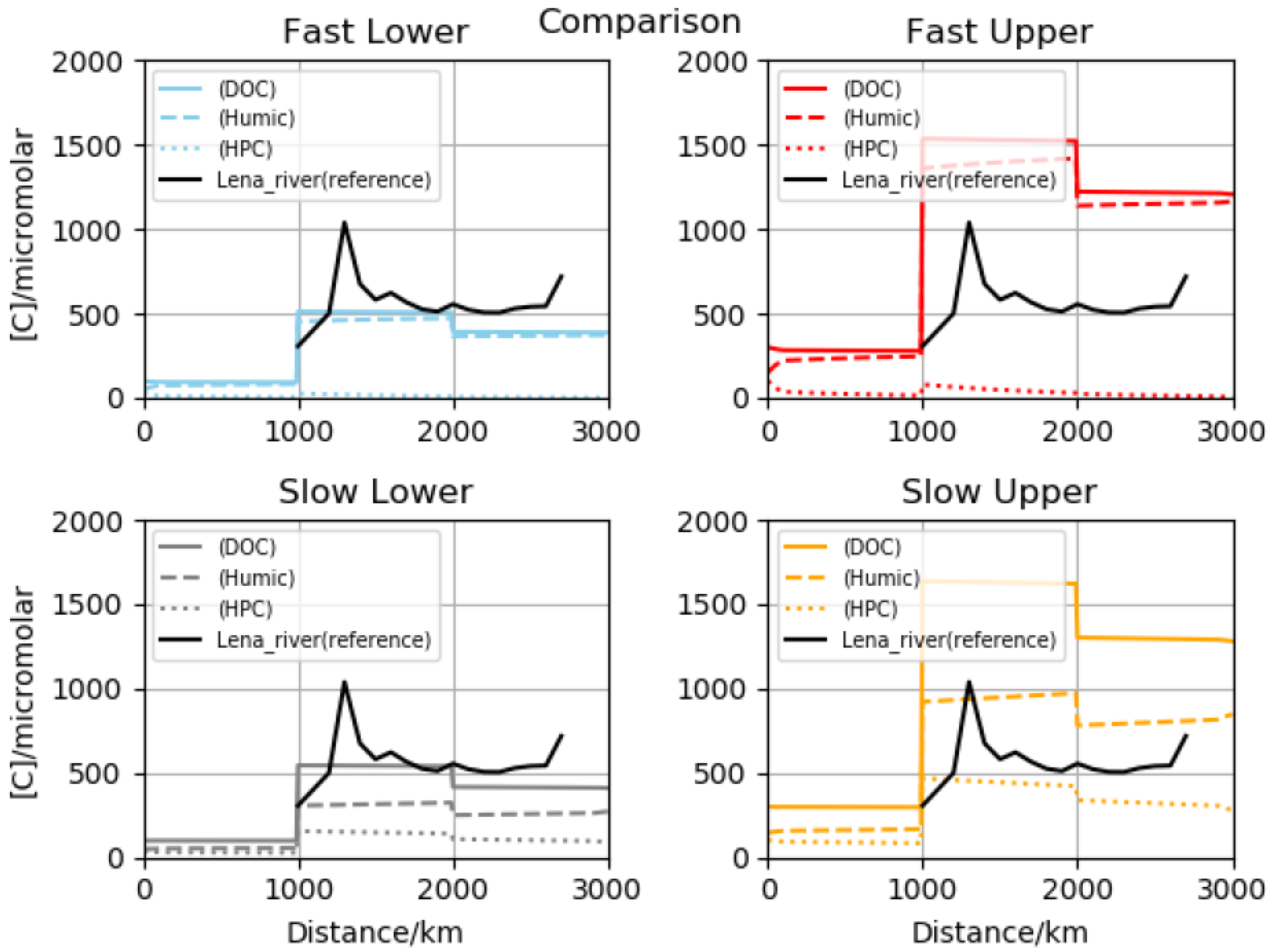This method dates from the early days of atmospheric chemistry, as various groups were dealing with numerical stiffness in the gas phase [16]. However, it transposes readily to reactivity in natural waters. Several plots are presented for time-dependent, dissolved concentrations, both in terms of total carbon atoms and those associated with specific functionality. Four major initial scenarios were investigated with regard to the rates and initial concentrations. We call them fast lower, fast upper, slow lower and slow upper, referring to the choice of chemical processes and soil-to-stream initializations. The slow and fast situations are the ratio for our generic, master-constant-based time scales to one another over an order of magnitude. For best-fit contours of the total organics, multiple panels are offered for inspection including the time evolution of a proteinaceous group, the carbohydrate collection, lipids as a family and also a phenolic category along with light absorbers. Total, humic and polycondensate values are sometimes appended as reference points, since concentrations vary by orders of magnitude. Comparisons are presented with data for overall dissolved carbon along the river course, and then for key polymer types at the mouth.

In concluding sections, we review the full computational logic and our results. For each macromolecular class, it is possible to simulate time evolution along a lengthy river coordinate by accounting for mixing, with seasonal chemical transformations superimposed on fresh water transit times [9,12]. This suggests the possibility for incorporating more detail through networks based on realistic hydrology. Concentrations at the river mouth are compared with measurement data given standard statistical formats [17], and through this strategy, we show that the coupled mixing and reactive processes illuminate functionality as well as total solute carbon. Concentrations at the delta mouth greatly exceed levels for the open Arctic Ocean in most cases. We thus argue that strong biophysical effects should be investigated along the coast. For example, adsorptive proteins may favor the marine–atmospheric interface with slowing to gas or momentum transfer [2], while sugar chains co-adsorb to hydrophilic groups from below [18]. Lipids will contribute to amphiphilicity as well, and organic chromophores extract light passing downward which might otherwise be available to support bioproduction [1]. In general, we evaluate multiple organic classes against quantifiable thresholds for coastal physical influence.

The text ends with the development of a simple box model analysis for plume dilution into the major marine receptor, which is along-shore flow with recirculation. The relationship is configured first at a regional scale, based on salinity considerations [19], then focused against the Arctic coastline with an estimated spreading distance derived from horizontal diffusivity [19,20,21]. It is possible through just a few simple equations to bracket the potential for product concentration patterns to distribute widely depending on lifetime. However, simultaneously, it is clear that biophysical impacts must ultimately be assessed in an interactive and geographically consistent manner. Detailed mixing chemistry then reactive dynamics should be continued from headwaters through tributary–distributary systems out to the turbulent plume regime.

2. Background

Dissolved organics in natural waters are most often studied from the global perspective as a counterpoint to oxidized carbon atoms. Reduced forms may be considered a vast reservoir sequestering material from the carbonate, so that there is no participation in the sea–air interchange as CO₂ [11]. This is just as true for terrestrial inputs as for marine products, and much effort has gone into sorting the two classes from one another [9]. In fact, land tracers such as lipid biomarkers and lignin-derived aromatics can be used to achieve separation, and we will track some of them here in a secondary fashion as vegetation derivatives. Examples include the syringyl and vanillyl phenols, which are specific to tundra and forest, respectively [12]. Continental sources are distinct from their marine counterparts in ways that reflect metabolism and lifestyle requirements. In addition to cytosol content such as protein, polysaccharide and lipid [15], one must account for structural support including cellulose and lignin. We adopt global average litter proportions for the various vegetation categories, applying them as boreal averages [9].

Structural carbohydrates and network aromatics can be set aside as solids which remain largely inert [11]. Most proteins and lipids, on the other hand, are not only soluble but become surface active at the micromolar level (by carbon atom accounting, which we use consistently). Polysaccharides co-adsorb at or near the water–air interface. Hydrophilic groups are targeted, with divalent cations operating as electrostatic bridging agents [18]. All of our dissolved forms are inherently partially oxidized, and furthermore they degrade near the atmosphere to generate precursors to volatile organic compounds (VOCs). Such transitions can actually be driven by photochemistry isolated to the water–air microlayer, at thicknesses as small as a monolayer or a single carbon–carbon bond [2,4]. Example gases include formaldehyde derivatives, as well as glyoxal and low molecular weight acids. Resins, tannins and waxes are present at trace quantities in the soil, but concentrations are typically low enough that we can avoid them preliminarily [9]. Isoprene and terpenoids must enter flowing fresh waters continually along the banks of coniferous systems, but since some are immediately volatile in and of themselves, we anticipate rapid ventilation [22,23]. Only a handful of experiments are devoted to them here. Our tactic in the case of, for example, monoterpenes or related compounds is to allow fast decay toward the atmospheric Henry’s Law equilibrium. Saturation concentrations should be forced to high by regional gas phase plumes during the growing season, since northern latitudes are heavily forested.

Climate change significance of the DOC will be strongly amplified in the Arctic, for a variety of reasons, that will prove relevant to our modeling. These are nicely summarized in the introduction to one of our more important open water references [1], and further with respect to terrestrial ecotone shifts by Frey and McClelland [7]. Seasonal discharge will naturally follow patterns of the regional hydrological cycle for a given water shed. Permafrost degradation and the migration of peat/boglands may either pulse-in or reduce organic injections during the melt, depending on local geochemical circumstances. Trends are likely to be complex on a decadal scale. However, of course, whatever the differential, it should maximize each spring. Early ice loss will increase photochemical and biological activity along much of the several thousand kilometer stream length, but especially in deltas and along the coast. Altered organic levels necessarily entail CDOM variation [1], and so also fluctuations in oceanic radiation attenuation. This effect is readily seen in satellite images to be a strong one. As aqueous concentrations adjust to regional warming and ecosystem change, they will alter a variety of fluxes into the polar marine atmosphere. At the sea–air boundary, evolving surfactant adsorption plays into both primary aerosol formation and the calming of capillarity, such that all manner of mass-energy transfer is in play [2,3,6,18]. Even metal-binding ligand levels could be tuned, as increased light availability and mixing drive primary production toward the pole. Enhanced nutrient utilization will expand small patches of iron limitation. In the present research, we attempt to lay the groundwork for the dynamic simulation of riverine DOC flow change, by introducing organic chemistry at a functional level. Moreover, we test for physical significance by exploring extensions into coastline plumes and peripheral seas.

3. Definitions

Biologically driven carbon chemistry is extremely complex—second only to biology itself—so that careful definitions are demanded when entering our discussions. We adopted a marine perspective as the foundation, since this reflects our recent research background. However, we then worked back toward central Asia, since eventual goals are cross cutting and multidisciplinary relative to the Arctic Ocean biophysics. A conceptual starting point has been our experience with biosurfactants, acquired lately at the scale of the global sea–air interface [2,6,10,18]. By now, we have delved deeply enough into this topic to consider separately such specialized biopolymers as peptidoglycan, chitin, chitosan and the molecules of information [2,15]. However, within a few publications, earlier effort led us to focus on larger contributors to phytoplanktonic biomass—the broad classes protein, polysaccharide and lipid. Of these particular biomacromolecular types, the first and third turn out to be by orders of magnitude the most surface active [2,6]. Such behavior is a direct consequence of their metabolic responsibilities within the cell.

Moving upstream, one must naturally superimpose an understanding of unique terrestrial compounds and most especially, the ring structures of cellulose and lignin [9,11,12]. In the freshwater context, their pure forms are mainly subtractable because they are less soluble. There is, however, an important subtlety. Rigid, cyclic biopolymers can act as sources of aromaticity during the synthesis of humics, which are determined mainly operationally as a laboratory precipitate (or adsorbate) under acid conditions. Benner goes so far as to distinguish marine and terrestrial humic categories by this criterion [15]. The former are of modest molecular weight and are largely condensed from fresh phytoplanktonic cytosol, while the latter carry an extended double bonded signature from land. Aromaticity is a litmus test for diagnosing terrestrial fractions in the bulk ocean [9]. However, fragments of the fresh carbon linger as a backdrop. A key point in all cases is that active biopolymeric imprints from the inside of living cells must transition through concerted microbial–photochemical attack toward refractory forms [11]. The latter may well boast geologic lifetimes [15].

A kinetic formula found to be useful and realistic is just that of fresh degradation funneled through mixed polymeric intermediates [2,6,10,15]. Heterogeneous chains built up from random monomeric and substituent units exhibit aquatic residence times between those of fresh release and growing resistance. This sequence is common to research on the full spectrum of natural waters, from high altitude fresh systems to the deep sea [11]. We originally adopted it with regard to remote open ocean plumes flowing away from typical phytoplankton blooms. A central composition bin was referred to generically as processed carbon in this instance [6]. It was then further divided, into subsets specific to peptides, sugars and crossovers. We considered the family of lipids to constitute a short lived or labile fraction, based on direct coastal observations. However, in more mature surfactant studies, we were forced to deal with global cycling to and from the deep sea, and it proved preferable to define the intermediate pool in terms of mixed structures spreading across all surface waters. These were referred to as heteropolycondensates, partly for obvious etymological reasons but also following oceanographic community tradition [9,10,11,12,15].

Clearly, our group has been treating the notion of bioorganic intermediacy somewhat liberally, as emphasis shifts over regions of the total sea. Time constants and meanings have been varied as a matter of convenience, depending on the specific environmental situation. However, degradation consists ubiquitously of background enzymatic action augmented by photochemical breakdown given sunlight [9,12,15]. Microbial catalytic and high energy solar processes are the only means available to advance oxidation working against substantial activation energies for carbon bond rearrangement. The stabilization of diverse chains is merely an inescapable logical outcome, leading to intractable arrangements. In the present work, transformation steps of interest are those lying between the entry of soil carbon into headwaters, then operating during downhill flow along tributary–distributary networks, and finally blending as a kinetic continuum into polar seawater. Chemical intermediates are unavoidable and turn out to be instructive. In the present work, the term heteropolycondensate is invoked yet again but transferred upstream (and abbreviated HPC). This refers to the potential for riverine transition structures bridging toward further terrestrial humic accumulation.

Other entries in our interdisciplinary lexicon will perhaps be more familiar to the global aquatic chemist. We stipulate that stabilizing, acid-precipitable carbon dominates in the soil subsurface, well ahead of the river scheme [7,11]. This is just the standard humic mass, with its inherent aromaticity. The reader may wish to note that the term is itself operational, since it derives from the Latin root for “coming from the earth” (it is also thus technically a misnomer when applied to the sea). Our idealized boreal soil substrate is also infused with the fresh biomaterial of litter [9,11,12], and necessarily in between earth and sea we postulate HPC-style intermediates. These are permitted to decay toward their natural sinks in all reservoirs. From the river terminus, the language of chemical oceanography once again prevails, as we consider brackish media, coastal turbidity, sedimentation, the microfilm coating, an intense microbial food web, and the interaction of chromophore groups with incoming solar [1,9,10]. Regional photosynthesis, mixed layer heating and the field of pack ice become relevant. The overall framework is seen to be integrative of Earth system components that are most often modeled in isolation.

4. Early Geometry and Initial DOC Concentrations

Our model structure consists of one primary (first or longest) river starting from some mountainous area where gradients are steep and biogeochemical activity relatively low. We introduce two nodes or tributaries along the journey to the sea, one at a distance of 1000 km from the source and another at 2000 km. These inflows are simulated independently using the same kinetics. The reader should note a similarity to major Russian (Siberian) systems in general [12] and more specifically with regard to the Lena as in the experiments of Lara and others [13,14]. Plus, the resemblance to specific alternate networks such as the Yenisey and Ob is obvious since there will always be drainage of the central Asian plateau. Flow rates are set at the very rough round value of one meter per second following the extensive older USGS data from North America but consistent with modern satellite retrievals [24,25]. Thus, the total transit is made by any one Lagrangian chemistry box in about one month, in agreement with global hydrological averaging [11].

The plotted initial flow is usually taken to emanate from high elevation [8]. More concentrated solutes are added to the alpine headland value first at the one thousand milestone, and they are characteristic of familiar wetlands including both woodland and peat ecosystems [7]. This injection occurring early in our coarse network can be thought of as corresponding with the entry of the Vilyuy and its organics [13,14]. Then, an inflow is appended as filtered tundra vegetation [8]. Depending on the wetland type around primary streams, their initial concentrations are varied between round figures as discussed in the introduction. According to the group Shogren et al. [8], total dissolved organic concentrations for alpine and tundra watersheds fall respectively in the ranges of 30–300 versus 100–1000 micromolar. In the latter case, the most common measurements lie between 300 and 500. Seasonality is handled through local averaging. The Frey/McClelland data provide us with estimates for high solute forests or bogs, and the values may be compared with historical tabulations in, for example, Stumm and Morgan [11]. Roughly speaking, woodland, bog and peat fall in the interval from 500 to 6000 micromolar with peaks around 3000 [7].

We translate these results into a table defining major scenario types. Several critical assumptions then enter into choices for the initial concentrations assigned to individual organic classes. The proportion of humic substance should be greater than a majority based on global and Arctic observations reviewed by Hedges et al. [9] then later in Dittmar and Kattner [12]. The vegetative structural materials consisting mainly of cellulose and lignin are presumed insoluble and so are set aside. Fresh cellular biomacromolecules are then fractionated based on global estimates for overall ground level and soil plant matter, whether living or having transitioned to litter.

Subsurface organo-functionality becomes complex on land long before the river is reached. Ecosystem-level nutrient and water limitations dictate the columnar buildup of biomass, litter and soil reservoirs with the eventual output to the atmospheric and aqueous phases. We parameterized details here using selected observational constraints, aiming for coupling with land models as the calculations gain acceptance. About half of all above-ground carbon exists as the engineering cellulose or lignin, but several percent of the remainder can be assigned to the fresh biomacromolecular classes of protein, polysaccharide and lipid [9,11]. Cutins, tannins and specialty substances (molecules of communication, protection, information) are present at low levels as well. Of the latter, we deal in the present work only with the release of volatile organics. It is postulated that cellulose and lignin are somewhat inactive, while fresh amphiphiles and polymers are by contrast very mobile. Note that measurements historically indicate that riverine dissolved carbon is two thirds heterogeneous [9,11,12]. Hence, we initialize with protein–carbohydrate-lipid all rounded to 5 percent, which is conservation consistent. This logic implies at least a factor of uncertainty of two, but we feel it constitutes a reasonable starting point.

In some runs, the individual fresh concentrations were doubled or tripled without changing the total dissolved carbon, but agreement at the generic river outlet was sacrificed relative to measurements [12]. Preferred round values for all species are given in

Table 1. Initial class concentrations in micromolar of carbon atoms, leading with total dissolved organic carbon (DOC). Other abbreviations appearing are HPC—heteropolycondensate, and V—vanillyl or S—syringyl for the marker lignin phenolic compounds.

Components	Model Data
	Primary	Node 01	Node 02
DOC (measured)	30–300	500–6000	100–1000
DOC (initial)	100–300	1000–3000	300–1000
Proteins	5–15	50–150	15–50
Lipids	5–15	50–150	15–50
Carbohydrates	5–15	50–150	15–50
Humic	50–150	500–1500	150–500
HPC	35–105	350–1050	105–350
S-Phenol	0	0	3–10
V-Phenol	1–3	10–30	0

, below the summed or total concentrations. In the preliminary soil reactor, which is arbitrarily set to flow at 0.1 m/s over 100 km, the equilibration is permitted into oligomeric, monomeric and recondensate forms. Intermediate molecular weights are thus monitored explicitly and their curves will be obvious in our images. Note that the cytosol macromolecules are set equal to one another. This differs from global marine carbon and fresh biopolymer cycling, for which sixty–twenty–twenty ratios can usually be assumed [15]. Terrestrial material contains hemicellulose and waxes that tend to even out the macromolecular fractionation. Finally, we fill decrements up to 100% with heteropolycondensate which then decays to humic chains. All of this closely follows diagenetic evolution schemes outlined in the classic aqueous chemistry text Stumm and Morgan [11]. The vanillyl and syringyl phenols are superimposed at 1% concentration as biomarker examples, for exploration of taiga and tundra inputs, respectively.

5. Model Description and Mechanism

The model itself is a Lagrangian box or aqueous chemistry volume moving toward the sea at one meter per second. Exceptions occur at the start of the simulation and its end, where the flow is reduced to 0.1 m per second for 100 km. The slowing represents a soil reactor/processor and a matching (terminal) deltaic counterbalance. These artifices are intended for later refinement. We are now seeking interactions with land or delta model groups to provide accurate, regional time scales as constraints. The hope is to reciprocate by returning concentration relationships along the much longer intermediate web. Our chemical mechanism is described in the extensive network

Table 2. River chemical mechanism presented in textual form. Mainly, the rates shown are empirical high latitude marine to coastal values, while others may be relative and taken from rough global concentration relationships. The entire grouping is scaled slower in certain key runs as described.

Component	Source	Time Constant/Days	Products
Cellulose	Litter	(insoluble)	-
Lignin	Litter	(insoluble)	-
Protein	Cellular	10	Polypeptide
Polypeptide	Protein	3 × (10/13)	Amino acid (3 days) HPC (10 days)
Amino acid	Polypeptide	1	(Bacteria)
Polysaccharide	Cellular	30	Oligosaccharide
Oligosaccharide	Polysaccharide	10 × (10/11)	Monosaccharide (10 day) HPC (100 days)
Monosaccharide	Oligosaccharide	30	Inorganic C
Lipid	Cellular	3 × (10/13)	Inorganic C (3 days), HPC (10 days)
Heteropolycondensate (HPC)	See above right	10	Humic
Humic	HPC	Refractory	-
Vanillyl	Lignin (Taiga)	3	Inorganic C
Syringyl	Lignin (Tundra)	3	Inorganic C
Pigments (Chlorophyll)	Cellular	10	Porphyrin
Porphyrin	Pigments	10	Inorganic C
CDOM	Linear f(Prot, HPC, Humic, Chlor, Porph, V and S)
VOCI	Cellular	(ventilation)	Gas phase
VOCII	Photochemical	(ventilation)	Gas phase

. An arithmetic shorthand condenses branching across what is in fact a strictly unimolecular process set. For example, the term 3(10/13) means a slight speed-up relative to the faster of two loss channels given the coupling of 3 days with 10 days. This and any related factors apply in several cases.

Within our table entries, the reader will find a matrix of biomacromolecular types prominent in riverine chemical evolution, their sources as we define them, a master list of baseline time constants, and products. Timescales are temperature-independent open ocean values for coastlines hinging on the central figure ten days [10,15]. These are likely to prove faster than any along the boreal river path. Rates were therefore downgraded as sensitivity tests, and one becomes the preferred scenario. Microbial consumption tends to be the fastest removal, but it should nonetheless remain weak over the course [9,12]. Referencing is as follows: for cellulose, lignin and humic chains plus related physical properties, see the review by Hedges et al. [9]; for protein, polysaccharide, lipid and heteropolycondensate (HPC) Ogunro and colleagues are fairly thorough [10]; for polypeptides, amino acids, oligosaccharidic and monosaccharidic substances, the Benner overview is informative [15]; for vanillyl and syringyl phenols, Dittmar and Kattner discuss the background ecology [12]; for CDOM, pigments and porphyrin consult Stedmon et al. [1] plus the aquatic chemistry texts; and for VOC^II, Mungall and company [4] give examples of small species released into the Arctic atmosphere by irradiation.

The purpose of the table is really to provide a mental image of carbon flow, through the redox switching of degradation–stabilization. It actually constitutes an idealized set of fates, for overall biomacromolecular mass. For example, protein loss logically leads first to peptides then amino acid. Such conclusions are readily verified for boreal rivers per the detailed organic perspective of Dittmar and Kattner [12]. Routings are displayed schematically in our Figure 1 [11]. Pseudo-first order competitions occur at the branch points, leading to time scales given in days in the third table column. Some are semi-arbitrary, and derivations are available from the authors.

As Lagrangian integrations proceed, functionally resolved species are treated as independent over a time step in an exponential-form Euler, embodied by the quasi-steady state approximation or QSSA [16]. A summary of the equation set is offered just below. Here, the C_i are concentrations for some biomacromolecule of interest, while C_j(k) are those of others in the network, P and L represent the production term and loss constant, respectively, and the symbolic delta t is a short interval following the volume downstream. Since concentrations are updated one by one, mass conservation is only strictly maintained as the step size is reduced. A conclusion here will be that photochemistry and microbial action are relatively slow, so that stiffness is not a concern and we avoid linear algebraic inversion. In the present work, tests were conducted down to one second over the month-long simulations, but most runs advanced at one hundred seconds. Concentrations are always carried in micromolar of pure carbon, equivalent to elemental millimole/m³:

$$\frac{d{C}_i}{d{t}_{QSSA}}=P_i\left(C_j,C_k,\dots \right)-L_i\left(C_j,C_k,\dots \right)C_i$$

(1)

$$C_{i,t+\delta t}= \frac{P_i}{L_i} \left(1-e^{-L_i\delta t}\right)+ C_{i,t}{e}^{-L_i\delta t}$$

(2)

$$P_i,L_i fixed for \delta t$$

Several special cases need to be mentioned relating to the table kinetics. We postulated that cellulose and lignin are insoluble. This is supported by a history of observations [11], and aqueous equilibrium values are only of the nanomolar order. The polysaccharides are sometimes termed starch and they represent high molecular weight sugar chains. Specific monomer identities are given in Dittmar and Kattner [12] but none are tracked here—examples include glucose and mannose. The lipids are modeled as long chain saturated or double bonded fatty acids rather than triglycerides or phosphorus structures. Therefore, small amphiphiles are not considered to be polymeric and there is no need for an intermediate. Several biomarkers are included, e.g., the lignin-derived phenols which are vanillyl and syringyl aromatics. They are capable of representing upstream taiga and tundra ecosystems, and we set their initial concentrations at arbitrary unit percentages. The concept is to demonstrate the potential for organics to track terrestrial ecodynamics. We could consider adding marker lipids along with waxes such as cutin, but this will be reserved for later [9,12]. We also performed offline computations for two types of volatile—those formed early in the process within a soil reactor environment, plus late-comers attributable to photolysis in the river plume and extending out into the open sea. Mechanisms are described schematically in the table columns.

A major goal is to dynamically assess any biophysical influence the macromolecules may exert once they enter a generic marine mixed layer. Hence, we took special care to chemically characterize light absorbers. Pigments are represented first by standard chlorophyll, also given a round low value signifying that it must be present from the outset. We hypothesized that chlorophyll decays to its porphyrin ring, which remains optically active. Finally, we took a low percentage from each of the proteinaceous, humic and heteropolycondensate pools along with other pi-electron rings and defined the total to be chromophoric. CDOM is an especially apparent and readily monitored fraction of freshwater organics [1]. In fact, since its concentrations are not directly measured as a rule, we will deal in relative concentrations per absorption properties at the reference wavelength of 375 nanometers—normalizing to local DOC. Specifically, we associated the coefficient of 10 m⁻¹ with the total level of 1000 micromolar. It is possible to calculate a physical optical cross section from these figures (0.01 m²/millimole), and furthermore, to verify that only a small portion of the available carbon atoms need enter into the quantum mechanics of light extraction. The specific groups involved remain poorly understood.

Ultimately, radiation integrations should be performed along the wavelength coordinate, but for the moment, it is sufficient to note the following: Stedmon-type spectral slopes S as in [1] suggest little proportional change moving to 400 nm and perhaps an order of magnitude less in attenuation in the mid-PAR (blue photosynthetically available radiation, 500 nm). Control over penetration depth therefore remains strong relative to the reference point, as one moves toward the infrared. Stedmon et al. explored the details from an empirical standpoint with respect to the primary production, photochemistry, heating, ice retreat and more. Before moving on to the results, we conclude this section by reiterating a crucial simplification. Please bear in mind that all concentrations are documented here in units of micromolar-dissolved carbon atoms, regardless of the length of a polymeric or aliphatic chain. A kilodalton strand thus enhances the elemental molarity accordingly.

6. Results

6.1. Total Carbon and Reprocessed Forms

We performed four major experiments, with starting points as defined in the above initial concentration table. The simulations will be referred to as fast lower, fast upper, slow lower and slow upper. The meanings are meant to be self-evident, as for example in fast lower, we applied the coastal or master rates which are overestimates, along with reduced concentration values. The results of the four-part exercise are overviewed in Figure 2. Dissolved organic levels are most obviously determined by the idealized mixing state. The nodal blend is set at one to one in all baseline runs at all locations. As expected from Table 2, which incorporates net riverine sinks only for the trace volatiles, the total carbon can be roughly conserved except for mixing when plotted versus distance. Given the slow kinetics adopted for the lower images, recondensed heteropolymers and the humic endpoint themselves approach conservation to the zeroth order. However, rapid transformations in the alternate panels strongly impact the intermediate polymers, causing concentration divergence and near removal. Table 2 time constants are similar for the fresh biomacromolecules. Since such interconversions are not observed in nature [9,11,12], we eliminated the fast scenarios from further consideration.

On our upland thousand kilometers, the system concentrations for dissolved carbon lie between the initialization brackets, which are set to one and three hundred micromolar. By contrast, at the first confluence, with a (woodland–peat–bog) tributary bearing high solutes, levels jump dramatically and perhaps somewhat artificially in a stepwise manner. On the other hand, there is evidence in the real Arctic that pulses do occur [12,13,14] and we expect a “smoothing” toward staircase behavior as realistic networking is invoked. The largest concentrations are encountered in slow upper, due to the combination of mass and preservation factors. Values are roughly constant even for reactive chemical members because the master time of ten days was multiplied by an order of magnitude. Removals and transformations thus take place at a seasonal scale, while the hydrological environment purges itself in weeks.

The black curve in the center of each panel portrays a series of contemporary wet chemical determinations, as documented by the Lara group [12,13]. Their measurements began just beyond the isolated Siberian city of Yakutsk and extended past the Lena Pillars over several dozen roughly equally spaced stations, all the way to the vast delta. Data underlying the black trace were actually collected beginning only along Asian polar lowlands, so that the reader must take care in interpreting the patterns. No actual concentrations were obtained upstream relative to Yakutsk as a river port, and it is located at an elevation of only 100 m. Thus, any injections from mountain ecosystems are not directly represented. Furthermore, the black peak extending upwards along the y axis to over one thousand micromolar was really sampled upstream tens of kilometers relative to a confluence with the large tributary known as the Vilyuy [14]. It should therefore be viewed as a separate incoming source, and does not reflect subsequent mixing.

On the basis of the temporal and high-concentration factors displayed in Figure 2, we judge that our most realistic dynamic simulation is the one labeled slow lower. Total DOC is in close agreement with river campaign data since the only outlier is representative of a tributary. The subset of two heterogeneous organic classes behaves in a reasonable, less reactive manner. For the moment, the arguments are informal, but a more rigorous confirmation follows in our statistics section. Turnover rates for the constituents are quite low in the slow lower scenario due to the general time constant stretching applied. Given contrasts which can be drawn from the figure, therefore, we suggest that chemical processing is subdued for all of Table 2, following the course of any high flow rate boreal system. Mixing by contrast plays a dominant role in polar aquatic chemistry. We postulate that this is true from the moment of entry, from soils or runoff at altitude along freshwaters upstream and through to the delta. In the latter case, there is global evidence that organic decay may be rapid, for major components along distributaries and in reservoir features [1,9,12]. Along our selected aggregating system however, the combination of the addition with dilution explains major shifts. Thus, our work points to a significant opportunity for network modelers to interact with aquatic chemists.

A fifth potential run implies results so obvious that we did not display the plots, and in fact they would not be useful at this stage. It is possible and would not be entirely implausible to raise all time constants to infinity. This gives a non-chemical Arctic hydrosphere, and it is less than interesting but cannot currently be excluded. Naturally, under zero-reaction circumstances, one can simply lower initial Table 1 percentages for fresh biomacromolecules and arbitrarily match terminal measurements. However, the data from global soils [9], along the typical river circuit, and especially on the Asian floodplain [12] are consistent with modest processing in springtime even at high latitudes. It is clear that meandering transport in the delta regime sometimes leads to real removal [9]. Microbial and photochemical degradation definitely accelerate once open water is reached by the Siberian plumes [1,19]. Our position is that the complete exclusion of processing upstream would be artificial. For the moment, we allow Table 2 pathways to progress at the reduced pace. The option is always available to turn them off as dilution computations improve. Even under no-chemistry assumptions, the boreal marine plume will be dictated by soil and litter diagenesis, complex riverine networking and the preferences of oceanic microbial ecosystems. Thus, given either modest or inactive kinetics, channel combinations remain critical. It is trivial to carry both along into upcoming mixing exercises.

6.2. Major Biomacromolecular and Tracer Groups

From this point, we zoom on the slow lower simulation as the most valuable learning experience. Four further panels are now provided in Figure 3, and they dissect model evolution for most of our individual functionalities. Log scales are employed in order to emphasize the asymptotic behavior of intermediates such as the various oligomers. Slight decay tails are associated with the delta reactor. Several orders of magnitude are required to portray all species simultaneously. One effect of going logarithmic is to even out the reactivity for the major species, but this is not surprising since we have concluded that mixing drives the most change. We now provide an in-depth analysis of the compound patterns in the organically resolved figure. Species are sorted not only by family but also according to the eventual biophysical effect. The proteins are perhaps most important taken as surfactants, though they are permitted to contribute to light absorption as well [6,15]. Carbohydrates may co-adsorb in brine or salt water [18], and the formation of gels or colloids takes place both in water and within sea ice [5,9,11]. The lipid reaction set is relatively simple since we ignore trimers–polymers, and so space was available in this quadrant to portray the biomarker phenols (lower left). V and S concentrations are set semi-arbitrarily to the micromolar level, so that the main feature is a sudden jump on the entry of tundra byproducts at 2000 km. Chromophores are summed in part from subsets of other classes and mainly those with conjugated double bonding. The humic and heteropolycondensate profiles are repeated in a gray tones for orientation purposes. As aggregate stable products, they maintain high levels.

The protein class panel emphasizes decay along the chain from fresh polymeric forms (cytosol direct). Immediate products can be characterized as polypeptides, but our sequence culminates in the monomeric amino acids. There are several dozen types which could be accounted, but for the moment we treat R groups as indistinguishable. Amphiphilic effects tend to average over the primary structure. Oligomers and smaller are given zero concentrations initially, then buildup with time, mainly in the pre-reactor. The carbohydrate panel on the upper right includes oligosaccharides and monosaccharides as models for polymer degradation. Lipids and V-phenol begin with finite concentrations since both are present in high altitude litter, and they go on to react either photochemically or microbially but rapidly enough that early changes are evident even on our log scale. The S-phenol enters the flow later, its pulse obscured by gray gridding. This molecule acts independently since we adopt it as a tundra marker [12]. Both in the laboratory and real world, the S to V phenol ratio provides a quick interpretation of biotracer information.

CDOM supports a finite initial concentration since it combines fractional het-polymers, protein and total pigment (though the major component is chlorophyll). Porphyrins are chosen as an absorptive intermediate group likely under pigment decay. Humic and heteropolycondensate materials constitute the largest portion of dissolved carbon since conversion rates have been moderated. This is due not only to the zero-point, but also because mixed agglomerates integrate with time, over carbon mass harbored in the oligomer types (C gathering). As a result, high levels of heterogenous and aromatic polymer are maintained throughout the flow regime. Although we intend for gray curves to function mainly as a point of reference, they are of further importance to light absorption downstream due to their conjugation of double bonds. Heterogeous organics are included in the CDOM sum and contribute to the impact on coastal radiation penetration.

Starter concentrations for the proteins themselves, along with biopolymeric carbohydrates, intracellular lipids and the heteropolycondensates, are all fixed for mountainous soils of the first leg, and they are necessarily low due to the less intensive nature of high altitude ecosystems [8]. The first hundred kilometers of reaction is set aside as an idealized soil reactor, and the distance is really only an arbitrary small fraction of length because we have not yet consulted land modelers for geometric details. Nevertheless, since subsurface flow is slow relative to that of the main river, less-than-polymeric material is able to come into steady state. Decay and production rates are thus at their most visible on the left side of each image, in contrast with the main course. The reader will note several organic concentration shoulders evident early in the upland flow stretch.

Along the primary river and up to the 1000 km node (first link), substituent proteins, polypeptides and amino acids are subjected to photochemical and microbial degradation, but they do not show significant decreases in the concentration on our logarithmic scale. At the one thousand kilometer first-meeting point, we hypothesized that a tributary adjoins from woodland-, peat- or bog-dictated soils. Since entry is from litter-rich areas, local fresh water is enriched in all the organics [7]. Relatively high inputs are implied and they bolster concentrations via in-mixing, which is set for the sake of simplicity at one-to-one for all points. Sudden increases in concentration represent geometric averages, due to these rather severe dilution constraints. Between 1000 and 2000 km, changes are insignificant and in fact almost negligible in some cases. Again, we advise that a log scale has been adopted, but decay continues in the background at the mechanism-table time constants (times ten). At the 2000 km confluence, downward steps are indicated for each species or class. Here, we postulate the entry of a tributary carrying a characteristic tundra signature [8]. Relative organic concentrations are higher than those of mountains but lower than injections from any high solute zone. Observations for the Lena suggest that this possibility is not unrealistic [13,14]. Moreover, it makes sense relative to global geography and hydrology that large northern discharge systems begin their journey on the central Asian plateau of necessity, and they are joined on the Arctic steppe by short feeder subunits.

The (steep) roller coaster effect at our node points is exhibited on the log scales by all species in each panel, excluding our specialized portrayal of the syringyl compound—which appears in the lipid-marker image. The lignin phenolic varieties act primarily as biomarkers since they are present only at trace levels. We assumed as a startup expedient that their concentrations are low or zero in complementary boreal ecosystems (tundra versus taiga and vice versa). The potential for tracers to discriminate mixing is therefore demonstrated in a modeling context [12]. Turnover rates also play a role in determining the final concentrations at the mouth, but it is a weaker one. The imbalance of production and decay yields shallow gradients. Profiles are moderated somewhat given our choice of coordinate system, but the message is clear. Attention must be paid to the details of mixing parameters along the watercourse, with a superposition of modest photochemical or microbial degradation timescales perhaps being sufficient.

Table 3. River mouth values from the model with a summary of measurements at Arctic entryways, and for the surface of the open Arctic Ocean. Marine data are included since we will argue that high discharge plumes raise organic functional group levels above those required for regional biophysical effects. Units are the usual micromolar of carbon excluding CDOM absorption, which is proportional and detailed in the text.

Components	Model Output	Measurements
	River Mouth	River Mouth	Open Arctic
Proteins	11.8	12	1–2
Carbohydrates	17.0	25	10–20
Lipids	1.9	-	0.3–3
CDOM	5(1/m)	13	0.1–0.3

maps to the end points from the Figure 3 panels, and in it we compare the simulated outlet conditions against the end-of-river experiments. A column of data for open high latitude waters is also appended. Emphasis is placed on direct (diagenetically fresh) cellular contents such as the proteins, due to the likely surface activity, as well as the chromophores since light attenuation is relevant to primary production. References are as follows: river opening data are from the Dittmar and Kattner review [12] except CDOM which is taken from Stedmon et al. [1]. For the proteins, the measured values likely represent upper limits, since analytical hydrolysis frees some amino acid from the recondensate portion. Open water values are high latitude studies as summarized by Ogunro et al. [10], excepting again Stedmon et al. for attenuation. The conversion of chromophoric carbon to e-folding depths was handled as described in previous sections. For amino chains and carbohydrates, the results were fairly faithful. This is partly fortuitous of course given the global litter-soil initializations, but it may also be indicative of a realistic model design and decision process. We have not located river mouth data for the lipids and so this slot is left blank. Chromophores are characterized only by absorption coefficient, and our computations come in low relative to the Stedmon et al. data set. However, this was primarily due to the reliance on the lower Lena (Figure 2). Seasonality during the spring freshet pulse is strong and we have yet to account for it on a measurement by measurement basis [12]. All simulations are restricted to the months of May and June.

Notice that river mouth concentrations, whether modeled or measured, exceed typical surface seawater values. In fact, they surpass the expected threshold levels for strong biophysical effects. Elliott and coworkers, for example, summarized half saturation constants for natural interfacial adsorption, and the results have by now appeared in several sources [2,6,10]. In their discussion of a global biogeochemical equation of state, the transitions occur at 10 micromolar for the proteins and one half for the lipids. Carbohydrate co-adsorption must be expected when Langmuir coverage by the true amphiphiles is extensive (sugar hydroxyl groups bind via divalent cations [18]). CDOM concentrations are proxied in the present work by an inverse attenuation distance, and the river-coast differential is up to a factor of one hundred in terms of a₃₇₅. Informal wavelength extrapolations into the visible suggest that light penetration is likely to be limited for river-influenced coastal water [1]. This may be true in all the semi-isolated peripheral seas. Organic concentrations in high discharge boreal river plumes are so high that, prior to substantial dilution, intense influence on primary production seems likely.

7. Aqueous Volatile Organics as a Set of Special Cases

Volatile compounds which are the theme of the present issue deserve special mention at this point. They are closely related to our biomacromolecular families in that higher molecular weight carbon serves as a synthetic basis in many cases. Organic gases must have biochemical precursors, whether intra- or extracellular [4,26]. Marine phytoplankton produce isoprene as a byproduct during photosynthesis, and fluxes are often proportional to primary production [27]. Analog terrestrial processes are energized through ATP driving 3-PGA generation (glycerate 3-phosphate, a metabolic intermediate) [28]. With respect to river headwaters, we simulate VOC evolution as Henry’s Law equilibration, moving either upward or downward toward the dissolved steady state. Initially, degassing is prevented by physical capping since the atmosphere is not in intimate contact with the porous soil subsurface. There is no headspace for an aqueous phase tracer to enter. In several offline calculations, however, such barriers were removed. Analytical and Lagrangian boxes were uncapped then released for short excursions downstream, as loss occurs in minutes to hours so that full river lengths were unnecessary. Gas dynamics were portrayed as ventilation across the liquid laminar layer at the top of the turbulent upstream fluid. Isoprene served as the main model compound. In this sub-investigation, we focused first on the woodland tributary type identified at node one in Table 1, where for example conifer-derived terpenoids are likely to enter the aqueous soil environment [23,28]. The early input segment, however, also encompasses northern peats and bog-lands [7], so that volatile production has to be viewed as hypothetical. To address a broad spectrum of VOC concentrations, we studied the evolution for the entire scenario range low to upper, with local aqueous isoprene varied as a proportion of the total DOC. This provided a demonstration for variability that may be inherent to terrestrial aquatic trace gas chemistry.

We began by assuming that forest litter contains common terpenoids at parts per thousand of the total dissolved organic mass [23,28]. The figure is high and somewhat arbitrary. After an initial period of confinement, a head space was opened imagining that aqueous flow emerges from soil substrata. Ventilation rates were modeled via the standard laminar layer interface parameterization [22]—but with diffusivities and Henry’s Law constant values appropriate for isoprene [26]. We postulated a sharp rise in micromolarity in the spring as temperatures warmed, and related detritus underwent early diagenetic processing. However, further in the exercise, atmospheric mole fractions were varied upward from zero to those expected in the wake of a photosynthesizing forest [28]. The basic result was just this: because organic gases trapped in soil are volatile by definition and headwaters are shoal, the equilibration of the aqueous flow medium can be fast. We assumed a nominal baseline depth of one meter with sensitivity testing, and instantaneous turbulent mixing below the thin barrier. Ventilation into pristine air masses and equilibration with forest haze plumes were both extremely rapid. Time scales in fact were of the order of hours or less, so it is obvious that control is established locally along the course. The calculations were repeated for our other ecosystem choices of mountain and far northern tundra. Though concentrations differed widely, conclusions were similar.

To address the organic volatility of polar ocean systems, we estimated a mixed layer buildup for carbon volatile material released according to the photosynthetic rate, into the pool of water column DOC [26]. Refer to the mechanism table, near the bottom of our schematic list. Computational methods most often employed for large scale mapping follow either algorithms applied about a decade ago to dimethyl sulfide [29] or else to the full spectrum of dissolved organic functionality leading to surfactant buildup [10]. Levels sufficient for outflow from the sea surface are readily supported. Isoprene and the monoterpenes were taken as examples—they are rudimentary in molecular structure, containing only carbon and hydrogen atoms, plus high latitude sea–air flux determinations have been reviewed by the Shaw group [26] among others. We note especially that adsorbed organic monolayers are now thought to contribute independently to volatilization. As reported by Mungall et al. [4], the Arctic sea surface film is demonstrably an atmospheric source for low molecular weight carbon. This is true in particular for small oxygenated species such as acids, aldehydes, ketones, diols or glyoxal. Amplification must be anticipated in riverine coastal plumes [12].

8. Statistical Comparisons

In several cases we conducted statistical validation for the values obtained. A strong need for verification was dictated by numerous excursions from the evidence. This is perhaps obvious from a quick inspection of Figure 4, appended for purposes of introducing the present section. With biomacromolecular species types once again disaggregated, the fast upper run offers a direct counterpoint to the dampened rate-constant results. Such outcomes do not fare as well during a biopolymer-to-data comparison. The direct extrapolation of hypothetical coastal removal rates leads to substantial over-processing, and almost complete consumption in some instances. Monosaccharides collect carbon from their source polymers, acting as an integrated reservoir toward the end of the simulation. This has partly to do with the juxtaposition of hypothetical rate constants, but it is nonetheless artificial. Our judgment is that agreement with both experience and measurement is lost moving over the floodplain, into the delta and toward the outlet. An order of magnitude or more of micromolarity separates simulation from reality for some measurements in Table 3. The reader will recall that a nonchemical approach constitutes hidden scenario five—this would clearly err in the opposite direction if the global average litter composition were merely preserved [9].

In response to these issues, we performed point-by-point calculations contrasting the preferred baseline with a more complete suite of Asian river data. Experimental values filtered for incorporation extend beyond well known high discharges to moderate intensity flows of, for example, the Eurasian Indigirka, Pechora and Kolyma. While broad variation exists among the best studied sources, our nominal Lena calculations fall well inside the Arctic riverine envelope in most cases. The results are thus encouraging. However, data are still sparse and we hope to supplement them with modern web-based sources soon. As we extended the standard analyses across the Russian coastline for relevant biopolymers, clear indications emerged that our results have overall pan-Arctic validity. This is true despite their idealized (Lena-centric) nature. A summary is offered here in

Table 4. Standard analysis of dissolved carbon results divided into (1.) a left hand portion with the root mean square (RMS) taken relative to the total organic measurements downstream of Yakutsk, and (2.) the total plus functional group distributions at many peripheral exits organized to the right. All values are in the micromolar of elemental carbon except CDOM as attenuation per meter.

Model Run	RMS (TDOC)	Group	Average	Standard Deviation
Fast Lower	192	TDOC	550	250
Fast Upper	824	Proteins	11.5	3.5
Slow Lower	143	Carbohydrates	25.2	10.6
Slow Upper	929	CDOM	8.6	4.1

, designed specifically to accompany the current statistics section. Some values are intentionally reiterated, while others differ slightly due to the more extensive geographic choices.

For total dissolved organic carbon, we worked along the spine of the original Lara set, moving northward from Yakutsk to the coast. Deviations were computed and the root mean square testing applied. Our initial qualitative selection of the lower level concentration set is confirmed—it is also quantitatively the best fit. River mouths were next contrasted with outlet data across the biochemical functional group spectrum but emphasizing amino acids and sugars, relative to a large number of drainages from the Lobbes and Engbrodt groups [30,31]. Biopolymer totals were computed by the re-addition of hydrolyzed amino concentrations or correspondingly for total neutral sugars. In the chromophore case, we relied upon averages from Stedmon et al. [1], which favor systems of greater name recognition (e.g., Ob or Yenisey). However, these are supplemented by the North American Yukon and MacKenzie. All values from the model output Table 3 fall within standard deviation envelopes, across a wide range of boreal chemistries. RMS computations were performed over N stations per the equation:

$$RMS= \sqrt{\frac{{{\displaystyle \sum }}_{i=1}^N{\left(x_{i,model}-x_{i,ref}\right)}^2}{N}}$$

(3)

9. Summary and Discussion

Aqueous organic chemistry transformations along an Arctic river are driven from their inception by terrestrial biota, but the oxidized group distributions are necessarily complex. Functionality will be conserved to some extent heading downstream, with release into coastal waters where solutes impact regional biophysics of the marine system. Examples include surfactant influence on aerosol and sea air transfer [2], and light penetration because biomacromolecules contain chromophores [1]. Thus, there is a potential for land ecosystems to communicate at a distance with oceanic analogs—by modulating mixing behaviors, composition and primary production in peripheral seas. To sort out this complex environmental chemical situation (simulate the effects), we developed a first-generation kinetic model arrayed along an idealized Siberian river. We investigated the dissolved organic composition in an obvious but unique manner, by insisting on functional resolution and then tracking the interplay between highly divergent structures. Protein, lipid, carbohydrate, heterogeneous recondensate, humic and fulvic substances are all treated. Furthermore, we subcategorized and carried both oligomeric and monomeric units where appropriate, while allowing for not only photochemical/microbial decay but also the random rebuilding of intermediate polymers [9,11].

The framework for our study is a numerical network mimicking the Russian Lena drainage [13,14], and extending to a length of 3000 km. We included two distinct input tributaries as a matter of demonstration, connecting with the main flow at 1000 and 2000 km from a hypothetical highland source. Transport and chemical reactivity are represented in a Lagrangian mode. Along the primary stretch and also tributaries, the processing of various organic molecules is simulated by analogy with the coastal ocean, which provided baseline rates [10]. However, these have been slowed on a sensitivity test basis to match total dissolved carbon measurements, and the best fit with actual data was achieved for the rates low enough that mixing becomes a dominant factor. The riverine organic mechanism we derived was perhaps the most detailed yet applied to boreal aqueous carbon cycling, but it is nonetheless compact and amenable to insertion into hydraulic codes. Major dissolved forms permitted to enter the river extend well beyond the macromolecules mentioned above to specific markers including (1.) terrestrial lignin phenols capable of distinguishing e.g., tundra, (2.) analogs for the volatile organics and most especially terpenoids plus small intermediate oxidation states, as well as (3.) CDOM apportioned from all dissolved organic matter [1,12,15]. Biotracers decompose to inorganics in our scheme, and absorbers become porphyrins in part since extinction is contributed by chlorophyll.

Four main lines of numerical experiment were developed, by varying initial soil-injected concentrations [7,8] as well as boreal aqueous turnover rates for the various species [9,10]. In several sets of runs, we applied the maximum possible soil levels from observation, and for two further groups, much lower startup values were assumed. These broad calculation families were labeled upper and lower versions, respectively. In sub-simulations, we adopted either reactivities equal to coastal estimates or reduced by a factor of ten. Excluding stable classes such as conserved organic carbon, temporal variation was significant. Comparison with the Lena data obtained downstream from Yakutsk [13] indicated that one particular combination may be somewhat superior—that termed slow lower. We performed comparisons with both total organics and outlet biomacromolecular determinations, and satisfactory agreement was obtained. Results were also placed in the context of pan-arctic data sets, and all preferred results fell inside the standard deviation envelopes. Stepping back to the full-length vantage point (highland-to-sea), we showed that in most cases concentrations are enriched across the delta–coast boundary. This is despite the complex input, mixing, dilution and processing. In fact, we argued that outlet levels may be biophysically significant, since known thresholds are surpassed for adsorbed coverage (surfactants in the Langmuir–Freundlich sense), primary organic aerosol emission mechanisms including the co-association of carbohydrates through metal cations [4,18], surface tension effects on sea–air transfer [2,6], light absorption [1,15] and more. Cutoffs documented in our reviews for marine film chemistry are roughly 10 and 0.1–1 micromolar bulk carbon for proteins and lipids, respectively. Moreover, we now have reason to believe that remote sensing will demonstrate the suppression of high latitude capillary waves in both hemispheres [32].

Although simulated and measured riverine concentrations are higher than those of Arctic seawater for any of the organic forms considered, questions remain regarding the areal extent of the plumes generated. Moreover, it is their (bio-)geographic area which will serve as an early indicator of ecological or economic importance. Indeed in the immediate vicinity of a deltaic or estuarine exit, dissolved carbon concentrations are necessarily at maximum. However, overall it is now necessary to begin mapping potential zones of oceanic physical influence. Dilution factors will exert themselves rapidly in the along-shore environment, and ultimately turbulent horizontal mixing drives communication with the free background. We anticipate that these issues must soon be addressed in coupled river input-general circulation models. To conclude, a preview is offered for river tracer distribution patterns. We constructed and estimated these in an analytical fashion. Coastal mixing calculations are now put forward at a back of the envelope level, and we propose to improve them as legitimately linked land–river–delta–plume simulations become available.

A flexible box model was designed for the quick assessment of plume dilution within an unspecified peripheral sea. For example, the Laptev can be seen as a receptacle constrained by Severnaya Zemlya and the New Siberian Islands, while the complete eastern Arctic Shelf is intensely fueled by multiple discharges [12,19]. In the equations just below, V are the volume flow rates associated with either assemblages of ocean currents which may be recycling (subscript o) or else river inputs (subscript r). Additional identifiers i/f signify initial and final states for transiting seawater. Lower case v subscripted “as” is restricted to the current velocity oriented along shore, and depth z always refers to the average mixed layer (ML). The K are just horizontal diffusion coefficients as often tabulated for coastal sites around the globe [20,33]. Moreover, letter t is a flexible time period capable of taking on several meanings, but here mainly defining an advection scale. Applying mass conservation and then minimal rearrangements, we obtain symmetrical relationships for the dilution of either marine or terrestrial inputs to aggregate pipe flow:

$$V_o{C}_{o,i}+V_r{C}_r=\left(V_o+V_r\right)C_{o,f}$$

(4)

$$\frac{C_{o,f}}{C_{o,i}}=\left(\frac{V_r}{V_o+V_r}\right)\left(\frac{C_r}{C_{o,i}}\right)+\left(\frac{V_o}{V_o+V_r}\right)$$

(5)

$$\frac{C_{o,f}}{C_r}=\left(\frac{V_o}{V_o+V_r}\right)\left(\frac{C_{o,i}}{C_r}\right)+\left(\frac{V_r}{V_o+V_r}\right)$$

(6)

$$V_o calibrated from salt, or=v_{as}{z}_{ML}\sqrt{Kt}$$

The first entry of this set is just a river-to-ocean tracer concentration balance in the simplest possible form. The next two summarize the linear relationships among concentration ratios. Quick tests such as C_r = 0 versus infinite, C_o,i = C_r can be used to check that the derived dilution ratios are sensible. In the last line, we point out that for rapid processing, it is more appropriate to consider local mixing.

One scheme for applying such relationships is to first calibrate against well understood stable substances. For example, minerals and salt constitute only minor components of Arctic river water [12]. Salinity values therefore drop dramatically along the brackish Asian coastline, from order 35 to 25 psu [19]. The ratio 5/7 falls out of the C_o,f/C_o,i expression as an approximation and leads to V_r/V_o = 2/5. One can use well known discharge rates for the Russian sector (several times 10⁴ m³/s [12]) and a scale volume of (1000 km)² by 30 m z_ML to verify a reasonable sub-basin refill/purge rate of ten years. Thus, we feel confident in moving on to assess the dissolved organics since the decay constant is long and comparable [19]. For shorter lived tracers it is necessary to use V_o computed along shore in the final expression. The limiting round figure inputs are 1 m/s, 30 m mixed layer depth, the central global (horizontal) eddy diffusivity of 10³ m²/s and the duration of one day implying a one hundred kilometer stretch of coastline, giving receptor flows of about 3 × 10⁵ m³/s. An individual spring river discharge peak reaches 3 × 10⁴ [12] so that V_r/V_o = 1/10. Final oceanic dilution can then be computed for both stable and transient tracers. Results are sampled in

Table 5. Input and output from the box river-to-coast mixing model developed in our discussion section, with comparisons to the data in the last column. Concentrations retain the standard chemistry units of micromolar with two exceptions—practical salinity units and for the chromophoric organics, we substitute the proportional absorption coefficient in per meter. Subscripts are fully defined in the text. Superscripts have the following significance: 2000 and 2100 are CE date-years denoting the recent contemporary era and a hypothetical globally warmed, amplified Arctic. Blank cells carry information downward from directly above.

	$\frac{{\mathit{V}}_{\mathit{r}}}{{\mathit{V}}_{\mathit{o}}}$	$\frac{{\mathit{V}}_{\mathit{o}}}{{\mathit{V}}_{\mathit{o}}+{\mathit{V}}_{\mathit{r}}}$	$\frac{{\mathit{V}}_{\mathit{r}}}{{\mathit{V}}_{\mathit{o}}+{\mathit{V}}_{\mathit{r}}}$	Co,i (ao,i)	Cr (ar)	Co,f (ao,f)	Co,f (Data) (ao,f Data)
Salinity	2/5	5/7	2/7	35 psu	0 psu	25 psu	25 psu
TDOC2000				100	500	210	200
TDOC2100				100	1500	500
CDOMtest				0.1 abs	10 abs	2.9 abs	0.3 abs
vaszML(Kt)0.5	1/10	10/11	1/11
CDOM2000						1 abs
CDOM2100					30 abs	2.8 abs

, which explores many of the equation terms. References for abundance are [1,12,19].

Fractions and ratios in the table have what are sometimes obvious values, but the aim here is clarity. Note that in order to avoid clutter, we assume that blank cells repeat from neighbors above them. To the extent that our linear approximations reflect current and upcoming reality, salinity allows the calibration for the integrated dissolved organics. Agreement is excellent for full systems modeling and MIT data quoted in support [19]. For a world with global warming and permafrost/peat/bog destabilization, we assign an arbitrary increase in river DOC of a factor of three [7]. Coastal dissolved carbon jumps dramatically and a zeroth order guess would be that biophysical effects may scale. Chromophores are not adequately represented by the salinity model because they are relatively short lived—as little as one year [1]. So we compute an independent along-shore flow with updated local volume ratios. It applies to a single one hundred kilometer stretch downstream, and in some cases the major discharges are closely spaced so that there will be additivity. Even in the present day, light absorbers only dilute to about one per meter (375 nm) and given the ecosystem disruption, shorter scales are not inconceivable.

In conclusion, we now organize a set of broader factors arising, with respect to river-sourced organics as the Arctic thaws in coming decades. Our Lena model estimates likely apply to other prominent watersheds—Kolyma, Yenisey, Ob, Mackenzie, etc., with smaller systems intervening. The issues we have come across are presented here in bullet form, since they are numerous and interactive/overlapping. Our considered opinion is that it would be well worth the community asking:

-

What portion of ancient litter in permafrost remains in active, biomacromolecular forms? Are functions somehow preserved? Perhaps contemporary initial protein/lipid proportionalities do not translate to the millennial scale.

-

What portion of ancient carbon assigned to humics still actually behaves in sub-functional form, perhaps retaining absorptive or adsorbing capabilities? Humic acids are known to be oligomerically heterogenous. Relict segments could wield undue influence.

-

Can we faithfully simulate the chemical composition of future boreal soils? Is it necessary or even possible to portray millennial organic microbial processing?

-

Similar issues apply within the delta regime, as organics passing into the ocean to become pelagic tracers/contributors. High concentrations require that we take all nonlinearities seriously.

-

Will proportions of light absorbing groups evolve and redistribute? It seems unlikely that they would remain fixed as source ecosystems far upstream reconfigure.

-

Will sufficient organic mass be released from the high north to monolayer-cover the entire Arctic Ocean? More likely in variable interannual pulses, but perhaps at some heightened steady state?

-

Will mixed layer and film carbon reservoirs act as regional ultra-sources of critical atmospheric products: primary organic aerosol, low molecular weight (oxidized) carbon as VOC, or the eventual secondary organic aerosol (SOA)?

It is by now widely accepted that an ice-free Arctic lies only a few decades ahead [1,7]. While basic drivers of marine primary production are already under evaluation under the new world order (nutrients fertilizing phytoplankton), dissolved organic chemistry of the northern ocean will steadily intensify and is receiving but little model attention. It appears that the spreading of basin scale films/slicks and the potential darkening of the summer column cannot be precluded. Thus, the evolution of not only carbon dioxide fluxes but also those of other elemental carrier gases, organic aerosol, momentum, heat, and water vapor are all in play. The integrated effects would constitute a hemisphere-scale communication, from warming ice age ecosystems on the continents down to the Anthropocene northern sea. Information would be transmitted by detailed molecular structure, given a chained carbon alphabet. Thus, we propose that a little recognized need for the Arctic systems modeling community will soon be an incorporation of dynamic aqueous organic tracers well beyond the traditional DOC.

Our own family of boreal system simulators now includes several regionally and finely gridded ocean models, with competitive marine ecodynamics and seawater biogeochemistry mechanisms. However, the classification of the dissolved organic forms is just beginning to enter, and only at the level of gross stability (for example, semi-lability as in [10]). Both labile and refractory macromolecules are omitted, and this really means most forms except perhaps pure polysaccharides and a poorly defined small fragment of the open marine heteropolycondensate [6,10]. Model river inputs currently range from none at all in some versions of our Arctic code suite, leaving pelagic ecosystems to fend for themselves in fueling reduced carbon, through annual averages for inorganic mass, with some attention to the spring freshet. However, inconsistency is the rule, and we anticipate that Arctic ocean validation exercises will soon underscore a strong need for coupling land–river inputs.

The preferred organo–chemical kinetics scheme we developed, consisting of about a dozen mildly interacting structures, should blend smoothly into tributary, deltaic distributary, plume interface and coastal algorithms. Furthermore, the Asian river network appears to be mixing-dominated, and so it must also be closely defined by initialization working from the top. Functionally resolved models of boreal soil and permafrost composition must be consulted. Moreover, the continental in-flux of organics must finally be rectified with global marine biogeochemistry, which remains coarse at the pelagic entry point. Our own open-water projects have recently moved in this direction through the addition of independent DOC tracers. Our resolved biomacromolecules can be adjusted, for example, to represent the suite of surfactants, aerosol or trace gas sources plus even the chromophores.