High-Resolution COSMO-CLM Modeling and an Assessment of Mesoscale Features Caused by Coastal Parameters at Near-Shore Arctic Zones (Kara Sea)


Abstract
1. Introduction
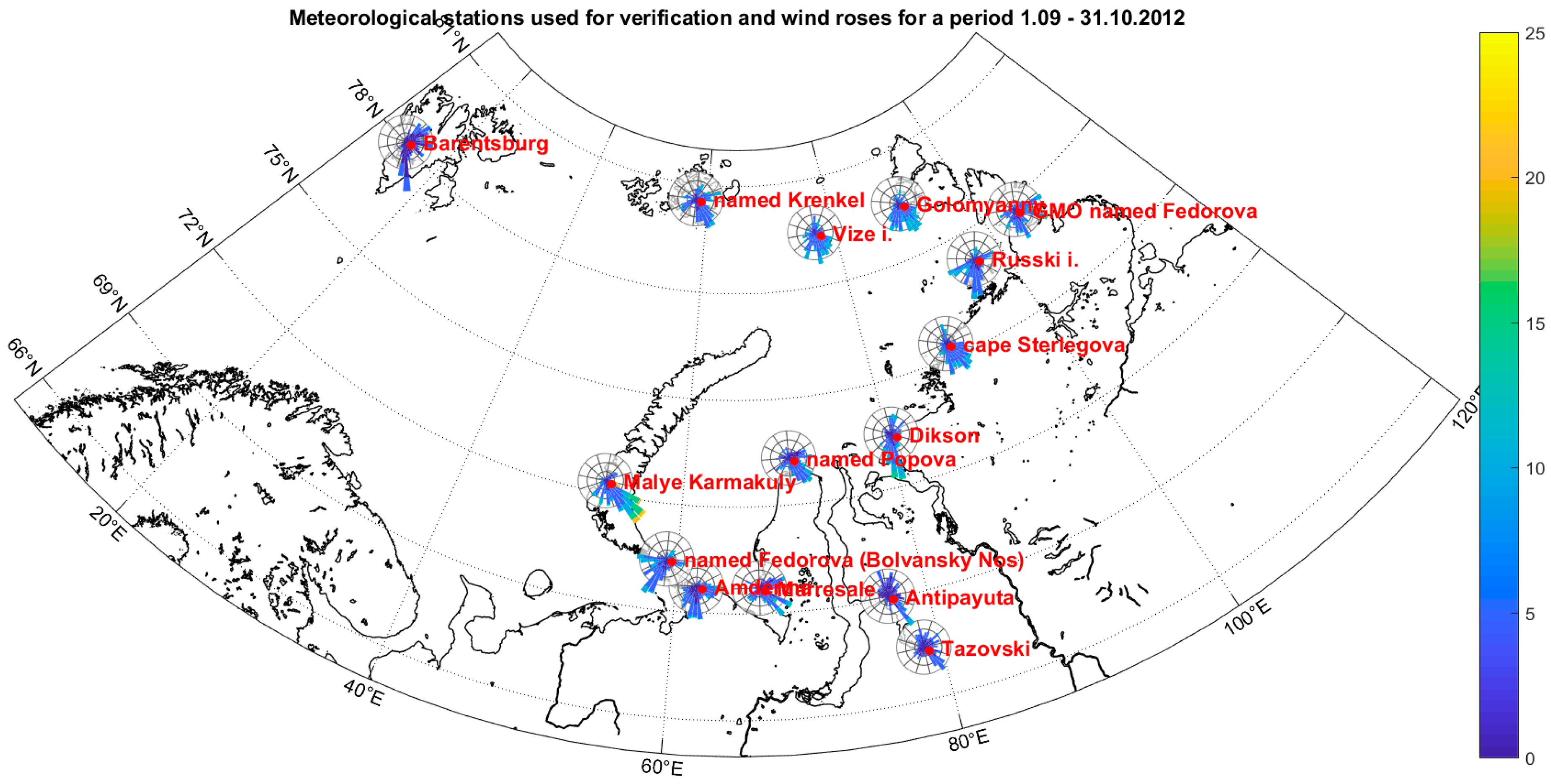
2. Data and Methods
2.1. Model Description
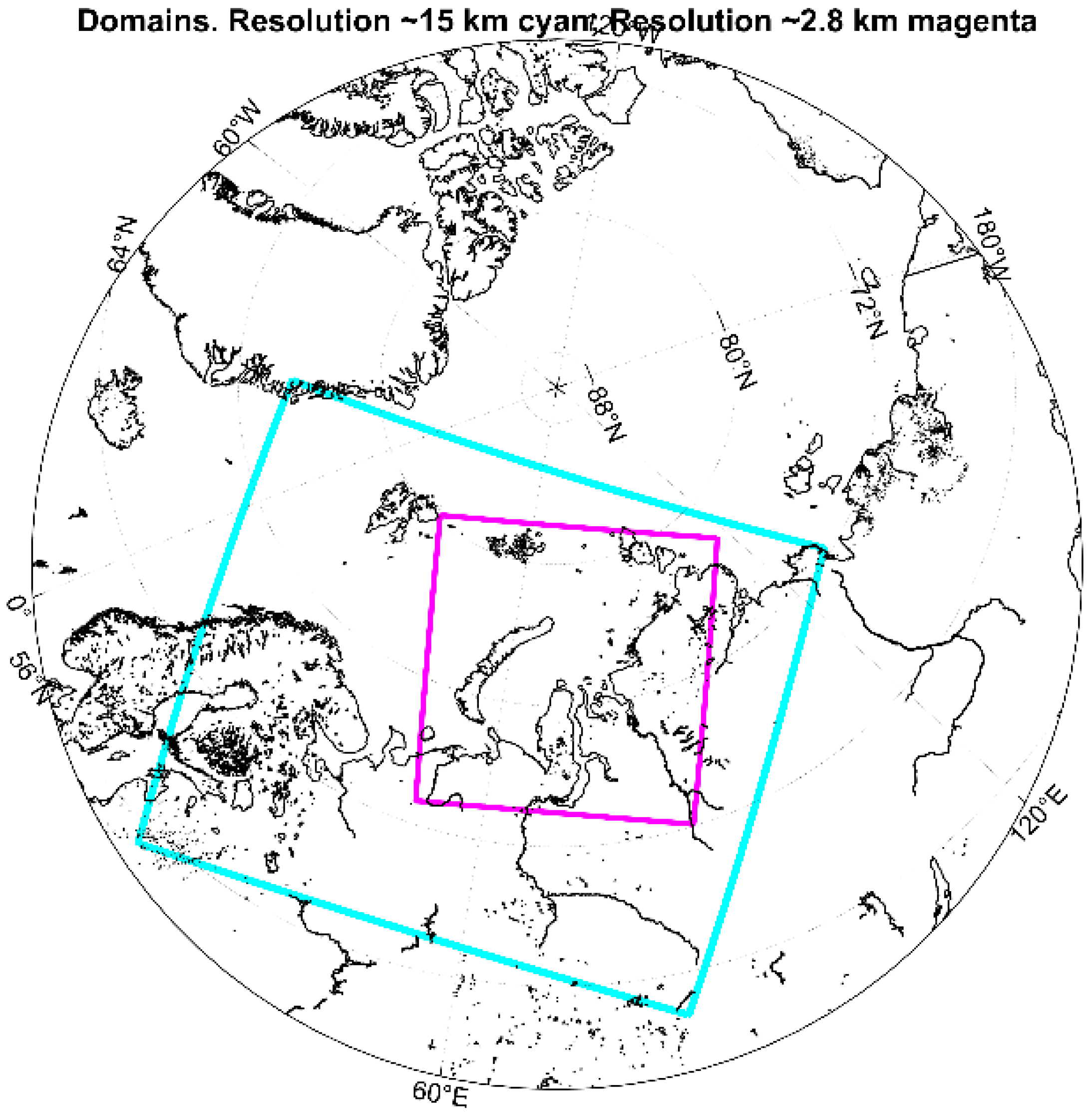
2.2. Experimental Design
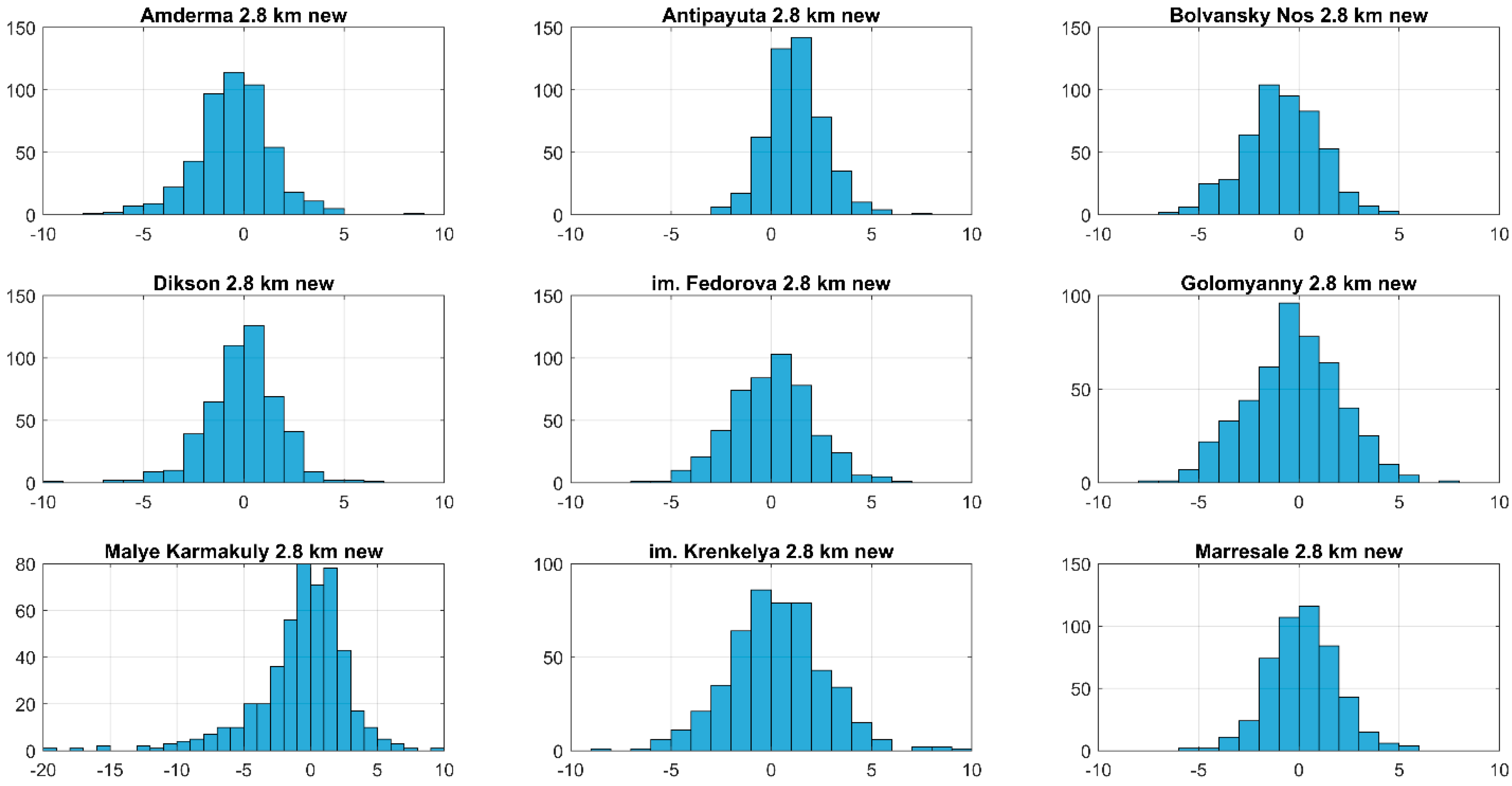
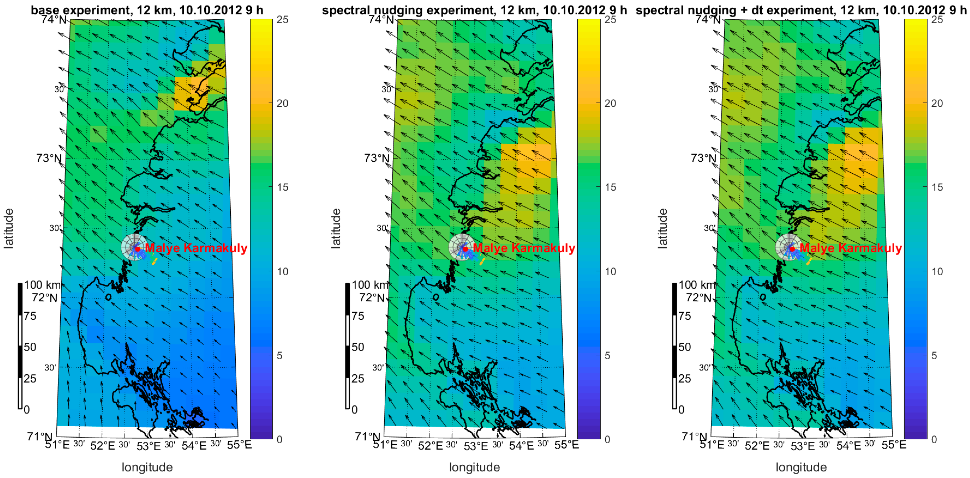
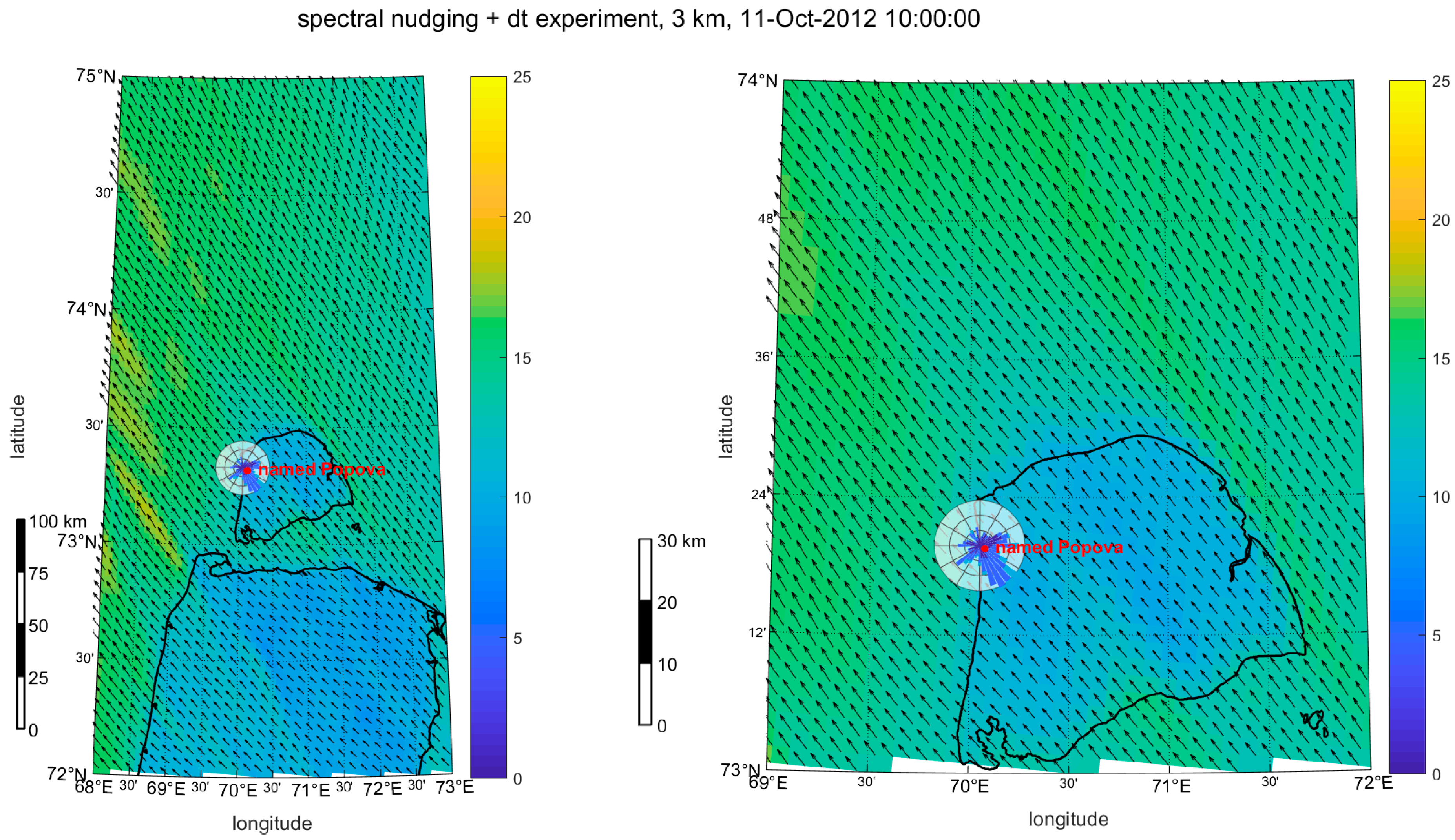
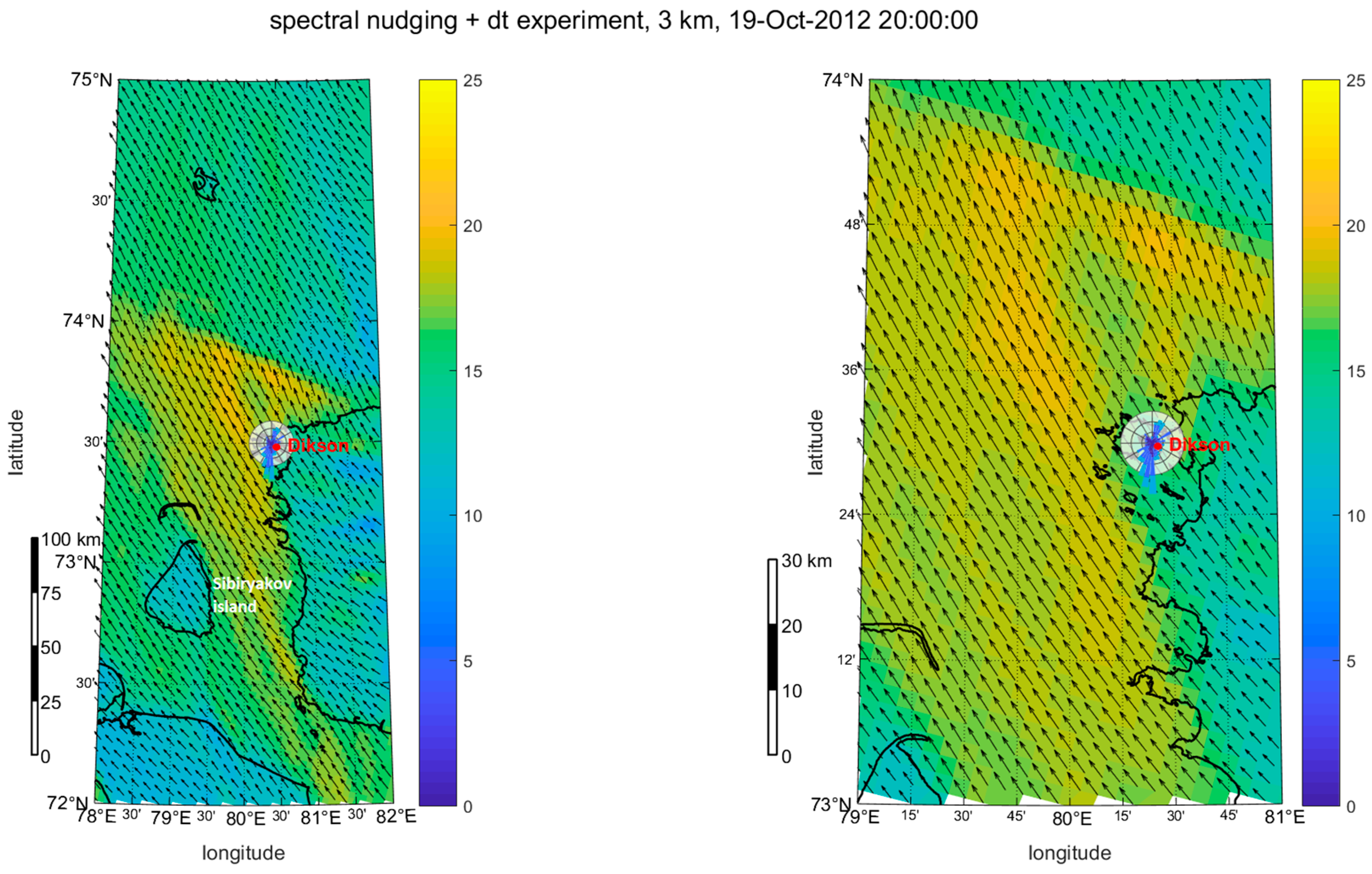
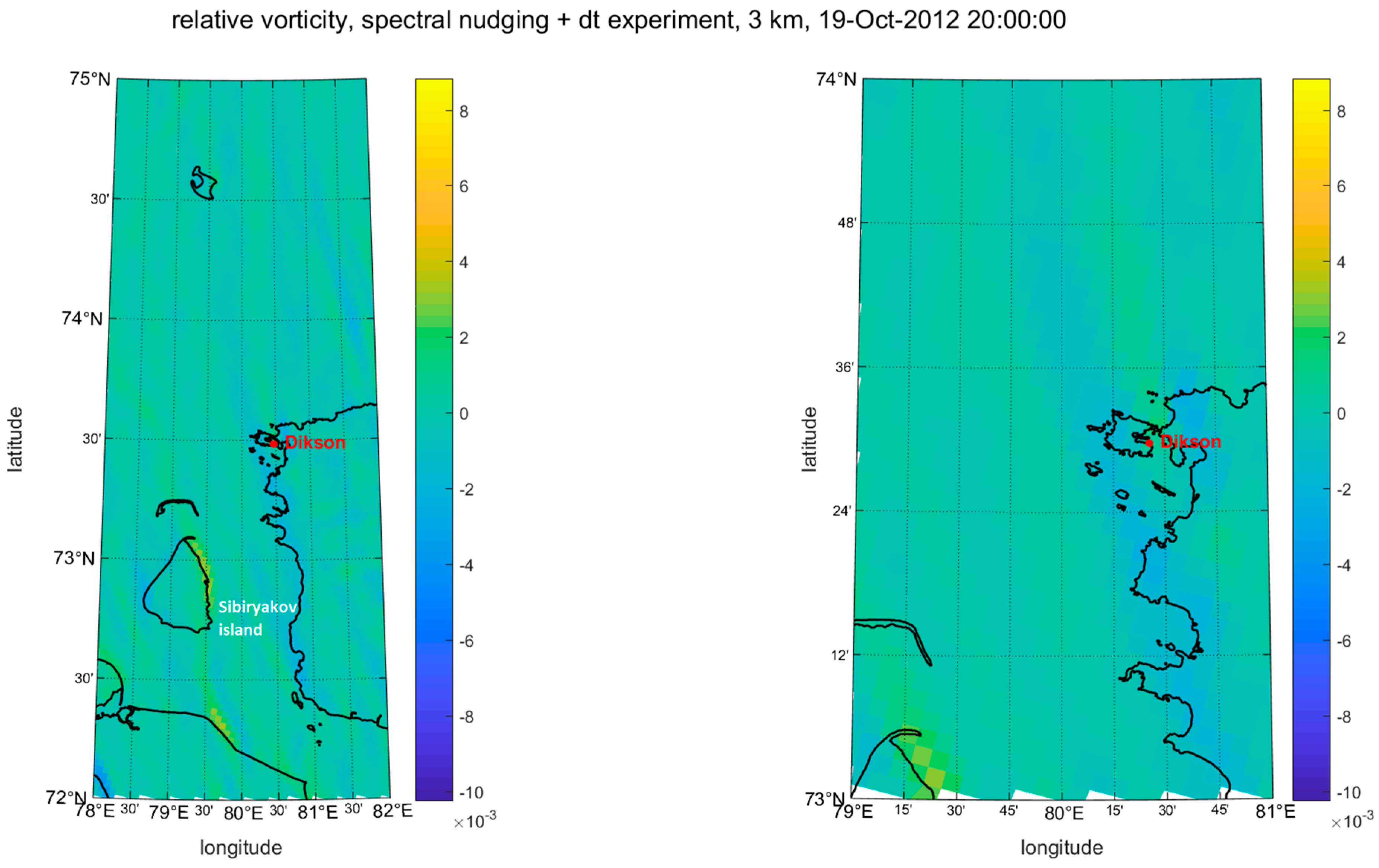
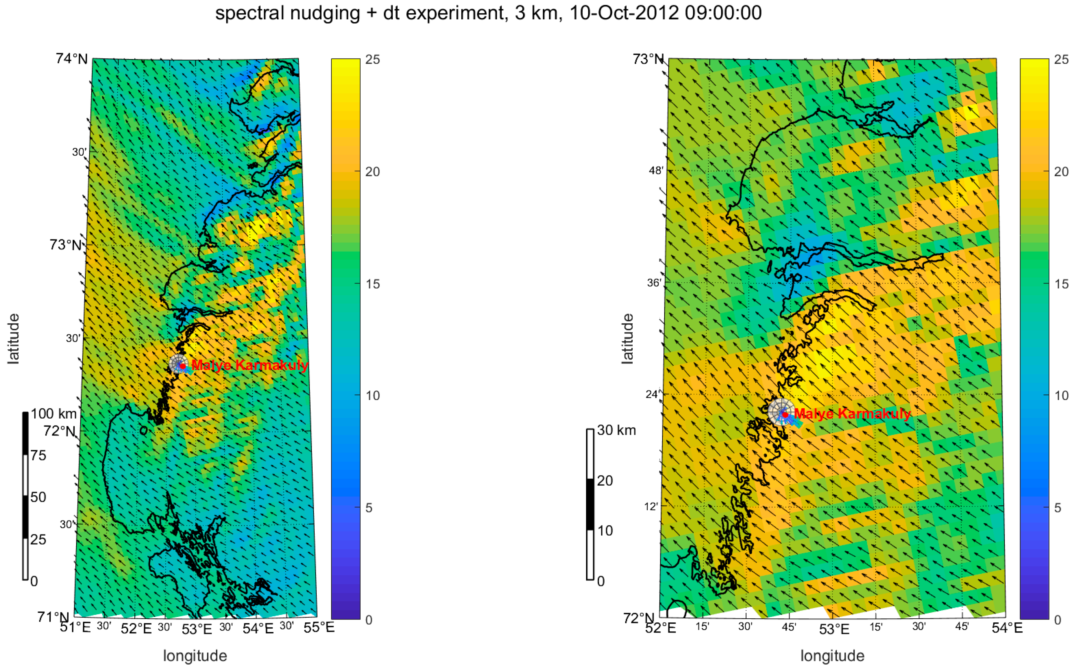
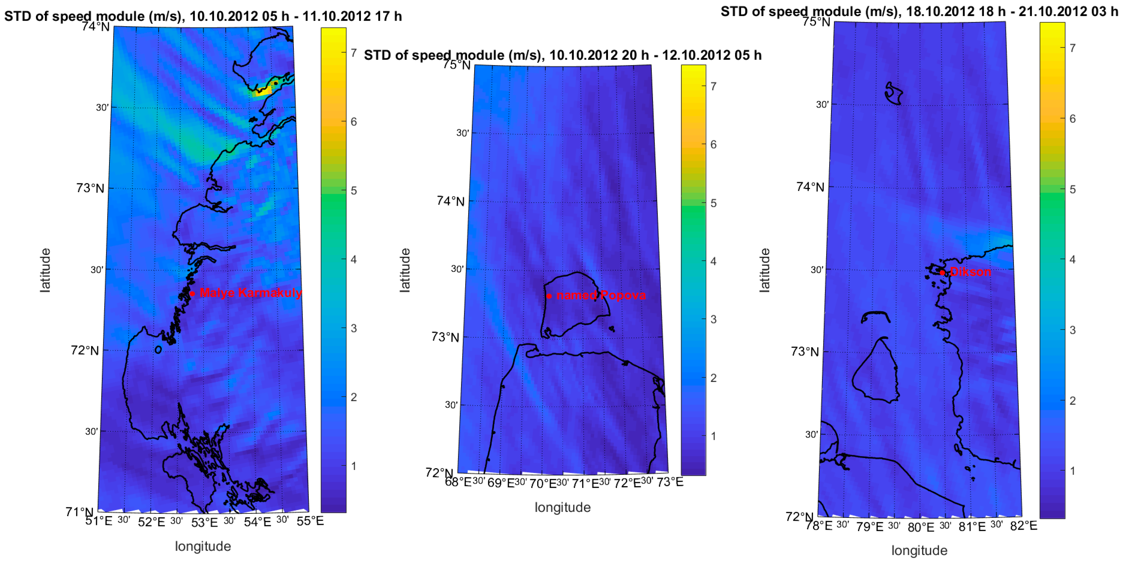
3. Results
4. Discussion
5. Conclusions
Supplementary Materials
Author Contributions
Funding
Acknowledgments
Conflicts of Interest
References
- Stocker, T.F.; Qin, D.; Plattner, G.-K.; Tignor, M.M.B.; Allen, S.K.; Boschung, J.; Nauels, A.; Xia, Y.; Bex, V.; Midgley, P.M.; et al. Climate change 2013: The Physical Science Basis. Contribution of Working Group I to the Fifth Assessment Report of the Intergovernmental Panel on Climate Change. 2013. Available online: https://www.ipcc.ch/site/assets/uploads/2018/03/WG1AR5_SummaryVolume_FINAL.pdf (accessed on 23 August 2020).
- Johannessen, O.M.; Kuzmina, S.; Bobylev, L.P.; Miles, M.W. Surface air temperature variability and trends in the Arctic: New amplification assessment and regionalization. Tellus 2016, 68A, 28234. [Google Scholar] [CrossRef]
- Walsh, J.E. Intensified warming of the Arctic: Causes and impacts on middle latitudes. Glob. Plan. Change 2014, 117, 52–63. [Google Scholar] [CrossRef]
- Budikova, D. Role of Arctic sea ice in global atmospheric circulation: A review. Glob. Plan. Change 2009, 68, 149–163. [Google Scholar] [CrossRef]
- Mori, M.; Watanabe, M.; Shiogama, H.; Inoue, J.; Kimoto, M. Robust Arctic sea-ice influence on the frequent Eurasian cold winters in past decades. Nat. Geosci. 2014, 7, 869–873. [Google Scholar] [CrossRef]
- Overland, J.; Francis, J.A.; Hall, R.; Hanna, E.; Kim, S.J.; Vihma, T. The melting Arctic and midlatitude weather patterns: Are they connected? J. Clim. 2015, 28, 7917–7932. [Google Scholar] [CrossRef]
- Screen, J.A.; Deser, C.; Simmonds, I. Local and remote controls on observed Arctic warming. GRL 2012, 39. [Google Scholar] [CrossRef]
- Cohen, J.; Screen, J.A.; Furtado, J.C.; Barlow, M.; Whittleston, D.; Coumou, D.; Francis, J.; Dethloff, K.; Entekhabi, D.; Overland, J.; et al. Recent Arctic amplification and extreme mid-latitude weather. Nat. Geosci. 2014, 7, 627–637. [Google Scholar] [CrossRef]
- Vihma, T. Effects of Arctic sea ice decline on weather and climate: A review. Surv. Geoph. 2014, 35, 1175–1214. [Google Scholar] [CrossRef]
- Bekryaev, R.V.; Polyakov, I.V.; Alexeev, V.A. Role of polar amplification in long-term surface air temperature variations and modern Arctic warming. J. Clim. 2010, 23, 3888–3906. [Google Scholar] [CrossRef]
- Barnes, E.A. Revisiting the evidence linking Arctic amplification to extreme weather in midlatitudes. GRL 2013, 40, 4734–4739. [Google Scholar] [CrossRef]
- Francis, J.A.; Vavrus, S.J. Evidence linking Arctic amplification to extreme weather in mid-latitudes. GRL 2012, 39. [Google Scholar] [CrossRef]
- Kohnemann, S.H.; Heinemann, G.; Bromwich, D.H.; Gutjahr, O. Extreme warming in the Kara Sea and Barents Sea during the winter period 2000–16. J. Clim. 2017, 30, 8913–8927. [Google Scholar] [CrossRef]
- Zhang, P.; Wu, Y.; Simpson, I.R.; Smith, K.L.; Zhang, X.; De, B.; Callaghan, P. A stratospheric pathway linking a colder Siberia to Barents-Kara Sea sea ice loss. Sci. Adv. 2018, 4, eaat6025. [Google Scholar] [CrossRef] [PubMed]
- Yang, X.Y.; Yuan, X.; Ting, M. Dynamical link between the Barents–Kara sea ice and the Arctic Oscillation. J. Clim. 2016, 29, 5103–5122. [Google Scholar] [CrossRef]
- Petoukhov, V.; Semenov, V.A. A link between reduced Barents-Kara sea ice and cold winter extremes over northern continents. J. Geoph. Res. Atmos. 2010, 115. [Google Scholar] [CrossRef]
- Kug, J.-S.; Jeong, J.-H.; Jang, Y.-S.; Kim, B.-M.; Folland, C.K.; Min, S.-K.; Son, S.-W. Two distinct influences of Arctic warming on cold winters over North America and East Asia. Nat. Geosci. 2015, 8, 759–762. [Google Scholar] [CrossRef]
- Outten, S.D.; Esau, I. A link between Arctic sea ice and recent cooling trends over Eurasia. Clim. Chang. 2012, 110, 1069–1075. [Google Scholar] [CrossRef]
- Orlanski, I. A rational subdivision of scales for atmospheric processes. BAMS 1975, 56, 527–530. [Google Scholar]
- Moore, G.W.K.; Renfrew, I.A. Tip jets and barrier winds: A QuikSCAT climatology of high wind speed events around Greenland. J. Clim. 2005, 18, 3713–3725. [Google Scholar] [CrossRef]
- Shestakova, A.A. Novaya Zemlya bora: The lee characteristics and the oncoming flow’s structure. Arct. Antarct. 2016, 2, 11–22. [Google Scholar] [CrossRef]
- Christakos, K.; Furevik, B.R.; Aarnes, O.J.; Breivik, Ø.; Tuomi, L.; Byrkjedal, Ø. The importance of wind forcing in fjord wave modelling. Ocean. Dyn. 2020, 70, 57–75. [Google Scholar] [CrossRef]
- Kilpeläinen, T.; Vihma, T.; Manninen, M.; Sjöblom, A.; Jakobson, E.; Palo, T.; Maturilli, M. Modelling the vertical structure of the atmospheric boundary layer over Arctic fjords in Svalbard. Q. J. R. Met. Soc. 2012, 138, 1867–1883. [Google Scholar] [CrossRef]
- Khvorostyanov, V.I.; Curry, J.A.; Gultepe, I.; Strawbridge, K. A springtime cloud over the Beaufort Sea polynya: Three-dimensional simulation with explicit spectral microphysics and comparison with observations. J. Geophys. Res. 2003, 108, 4296. [Google Scholar] [CrossRef]
- Gutjahr, O.; Heinemann, G. A model-based comparison of extreme winds in the Arctic and around Greenland. Int. J. Clim. 2018, 38, 5272–5292. [Google Scholar] [CrossRef]
- ReVelle, D.O.; Nilsson, E.D. Summertime low-level jets over the high-latitude Arctic Ocean. J. Appl. Met. Clim. 2008, 47, 1770–1784. [Google Scholar] [CrossRef]
- Gultepe, I.; Sharman, R.; Williams, P.; Zhou, B.; Ellrod, G.; Minnis, P.; Trier, S.; Griffin, S.; Yum, S.S.; Gharabaghi, B.; et al. A review of high impact weather for aviation meteorology. Pure Appl. Geoph. 2019, 176, 1869–1921. [Google Scholar] [CrossRef]
- Dee, D.P.; Uppala, S.M.; Simmons, A.J.; Berrisford, P.; Poli, P.; Kobayashi, S.; Andrae, U.; Balmaseda, M.A.; Balsamo, G.; Bauer, P.; et al. The ERA-Interim reanalysis: Configuration and performance of the data assimilation system. Q. J. R. Met. Soc. 2011, 137, 553–597. [Google Scholar] [CrossRef]
- Kalnay, E.; Kanamitsu, M.; Kistler, R.; Collins, W.; Deaven, D.; Gandin, L.; Iredell, M.; Saha, S.; White, G.; Woollen, J.; et al. The NCEP/NCAR 40-year reanalysis project. BAMS 1996, 77, 437–471. [Google Scholar] [CrossRef]
- Gelaro, R.; McCarty, W.; Suárez, M.J.; Todling, R.; Molod, A.; Takacs, L.; Randles, C.A.; Darmenov, A.; Bosilovich, M.G.; Reichle, R.; et al. The modern-era retrospective analysis for research and applications, version 2 (MERRA-2). J. Clim. 2017, 30, 5419–5454. [Google Scholar] [CrossRef]
- Hersbach, H.; Bell, B.; Berrisford, P.; Hirahara, S.; Horányi, A.; Muñoz-Sabater, J.; Nicolas, J.; Peubey, C.; Radu, R.; Schepers, D.; et al. The ERA5 global reanalysis. Q. J. R. Met. Soc. 2020, 146. [Google Scholar] [CrossRef]
- Saha, S.; Moorthi, S.; Pan, H.-L.; Wu, X.; Wang, J.; Nadiga, S.; Tripp, P.; Kistler, R.; Woollen, J.; Behringer, D.; et al. The NCEP climate forecast system reanalysis. BAMS 2010, 91, 1015. [Google Scholar] [CrossRef]
- Bromwich, D.; Kuo, Y.H.; Serreze, M.; Walsh, J.; Bai, L.S.; Barlage, M.; Hines, K.; Slater, A. Arctic system reanalysis: Call for community involvement. Eos. Trans. AGU 2010, 91, 13–14. [Google Scholar] [CrossRef]
- Bromwich, D.; Wilson, A.B.; Bai, L.; Liu, Z.; Barlage, M.; Shih, C.-F.; Maldonado, S.; Hines, K.M.; Wang, S.-H.; Woollen, J.; et al. The Arctic System Reanalysis, Version 2. BAMS 2018, 99, 805–828. [Google Scholar] [CrossRef]
- Hines, K.M.; Bromwich, D.H. Development and testing of Polar WRF. Part I: Greenland ice sheet meteorology. Mon. Weather Rev. 2008, 136, 1971–1989. [Google Scholar] [CrossRef]
- Bromwich, D.H.; Wilson, A.B.; Bai, L.S.; Moore, G.W.K.; Bauer, P. A comparison of the regional Arctic System Reanalysis and the global ERA-Interim Reanalysis for the Arctic. Q. J. R. Met. Soc. 2016, 142, 644–658. [Google Scholar] [CrossRef]
- Varentsov, M.I.; Verezemskaya, P.S.; Zabolotskikh, E.V.; Repina, I.A. Quality estimation of polar lows reproduction based on reanalysis data and regional climate modelling. Sovr. Problemy Distanc. Zondir. Zemli iz Kosmosa 2016, 13, 168–191. [Google Scholar] [CrossRef]
- Gavrikov, A.; Gulev, S.K.; Markina, M.; Tilinina, N.; Verezemskaya, P.; Barnier, B.; Dufour, A.; Zolina, O.; Zyulyaeva, Y.; Krinitskiy, M.; et al. RAS-NAAD: 40-yr High-Resolution North Atlantic Atmospheric Hindcast for Multipurpose Applications (New Dataset for the Regional Mesoscale Studies in the Atmosphere and the Ocean). J. Appl. Met. Clim. 2020, 59, 793–817. [Google Scholar] [CrossRef]
- Verezemskaya, P.S.; Stepanenko, V.M. Numerical simulation of the structure and evolution of a polar mesocyclone over the Kara Sea. Part 1. Model validation and estimation of instability mechanisms. Russ. Meteorol. Hydrol. 2016, 41, 425–434. [Google Scholar] [CrossRef]
- Diansky, N.; Fomin, V.; Kabatchenko, I.; Gusev, A. Numerical simulation of circulation in Kara and Pechora Seas using the system of operational diagnosis and forecast of the marine dynamics. EGUGA 2015, 4, 13370. [Google Scholar]
- Semenov, A.; Zhang, X.; Rinke, A.; Dorn, W.; Dethloff, K. Arctic intense summer storms and their impacts on sea ice—A regional climate modeling study. Atmosphere 2019, 10, 218. [Google Scholar] [CrossRef]
- Information about CLM-Community. Available online: https://wiki.coast.hzg.de/clmcom (accessed on 15 August 2020).
- Böhm, U.; Kücken, M.; Ahrens, W.; Block, A.; Hauffe, D.; Keuler, K.; Rockel, B.; Will, A. CLM–The Climate Version of LM: Brief Description and Long-Term Applications. COSMO Newslett. 2006, 6, 225–235. [Google Scholar]
- Rockel, B.; Geyer, B. The performance of the regional climate model CLM in different climate regions, based on the example of precipitation. Met. Zeitsch. 2008, 17, 487–498. [Google Scholar] [CrossRef]
- Arakawa, A.; Lamb, V.R. Computational design of the basic dynamical processes of the UCLA general circulation model. Meth. Comp. Phys. 1977, 17, 173–265. [Google Scholar]
- Gal-Chen, T.; Somerville, R.C.J. On the use of a coordinate transformation for the solution of the Navier-Stokes equations. J. Comp. Phys. 1975, 17, 209–228. [Google Scholar] [CrossRef]
- Schär, C.; Leuenberger, D.; Fuhrer, O.; Lüthi, D.; Girard, C. A new terrain-following vertical coordinate formulation for atmospheric prediction models. Mon. Weather Rev. 2002, 130, 2459–2480. [Google Scholar] [CrossRef]
- Ritter, B.; Geleyn, J.F. A comprehensive radiation scheme for numerical weather prediction models with potential applications in climate simulations. Mon. Weather Rev. 1992, 120, 303–325. [Google Scholar] [CrossRef]
- Tiedtke, M. A comprehensive mass flux scheme for cumulus parameterization in large-scale models. Mon. Weather Rev. 1989, 117, 1779–1800. [Google Scholar] [CrossRef]
- Klemp, J.B.; Durran, D.R. An upper boundary condition permitting internal gravity wave radiation in numerical mesoscale models. Mon. Weather Rev. 1983, 111, 430–444. [Google Scholar] [CrossRef]
- Skamarock, W.C.; Klemp, J.B. The stability of time-split numerical methods for the hydrostatic and the nonhydrostatic elastic equations. Mon. Weather Rev. 1992, 120, 2109–2127. [Google Scholar] [CrossRef]
- Core Documentation of the COSMO Model. Available online: http://www.cosmo-model.org/content/model/documentation/core/default.htm (accessed on 9 August 2020).
- Asensio, H.; Messmer, M.; Lüthi, D.; Osterried, K. External Parameters for Numerical Weather Prediction and Climate Application EXTPAR v5_0. User and Implementation Guide. Available online: http://www.cosmo-model.org/content/support/software/ethz/EXTPAR_user_and_implementation_manual_202003.pdf (accessed on 16 November 2018).
- Schulz, J.-P.; Heise, E. A new scheme for diagnosing near-surface convective gusts. COSMO Newslett. 2003, 3, 221–225. [Google Scholar]
- Platonov, V.S.; Varentsov, M.I. Supercomputer technologies as a tool for high-resolution atmospheric modelling towards the climatological timescales. Supercomp. Front. Innov. 2018, 5, 107–110. [Google Scholar] [CrossRef]
- Chen, F.; von Storch, H. Trends and Variability of North Pacific Polar Lows. Adv. Met. 2013, 13, 1–11. [Google Scholar] [CrossRef]
- Haas, R.; Pinto, J.G. A combined statistical and dynamical approach for downscaling large-scale footprints of European windstorms. GRL 2012, 39, 1–6. [Google Scholar] [CrossRef]
- Kotlarski, S.; Keuler, K.; Christensen, O.B.; Colette, A.; Déqué, M.; Gobiet, A.; Goergen, K.; Jacob, D.; Lüthi, D.; van Meijgaard, E.; et al. Regional climate modeling on European scales: A joint standard evaluation of the EURO-CORDEX RCM ensemble. Geosci. Model. Dev. 2014, 7, 1297–1333. [Google Scholar] [CrossRef]
- Geyer, B. High-resolution atmospheric reconstruction for Europe 1948–2012: CoastDat2. Earth Syst. Sci. Data 2014, 6, 147–164. [Google Scholar] [CrossRef]
- Hackenbruch, J.; Schädler, G.; Schipper, J.W. Added value of high-resolution regional climate simulations for regional impact studies. Met. Zeitsch. 2016, 25, 291–304. [Google Scholar] [CrossRef]
- Keuler, K.; Radtke, K.; Kotlarski, S.; Lüthi, D. Regional climate change over Europe in COSMO-CLM: Influence of emission scenario and driving global model. Met. Zeitsch. 2016, 121–136. [Google Scholar] [CrossRef]
- Kislov, A.V.; Rivin, G.S.; Platonov, V.S.; Varentsov, M.I.; Rozinkina, I.A.; Nikitin, M.A.; Chumakov, M.M. Mesoscale atmospheric modeling of extreme velocities over the sea of Okhotsk and Sakhalin. Izv. Atm. Ocean. Phys. 2018, 54, 322–326. [Google Scholar] [CrossRef]
- Platonov, V.; Kislov, A.; Rivin, G.; Varentsov, M.; Rozinkina, I.; Nikitin, M.; Chumakov, M. Mesoscale atmospheric modelling technology as a tool for creating a long-term meteorological dataset. IOP Conf. Series Earth Env. Sci. 2017, 96. [Google Scholar] [CrossRef]
- Platonov, V.; Varentsov, M. Creation of the long-term high-resolution hydrometeorological archive for Russian Arctic: Methodology and first results. IOP Conf. Series Earth Env. Sci. 2019, 386. [Google Scholar] [CrossRef]
- Luettich, R.A.; Westerink, J.J. Formulation and Numerical Implementation of the 2D/3D ADCIRC Finite Element Model Version 44.XX. p. 74. Available online: https://www.aquaveo.com/software/sms-adcirc (accessed on 4 October 2020).
- Bucchignani, E.; Montesarchio, M.; Zollo, A.L.; Mercogliano, P. High-resolution climate simulations with COSMO-CLM over Italy: Performance evaluation and climate projections for the 21st century. Int. J. Clim. 2016, 6, 735–756. [Google Scholar] [CrossRef]
- Parkinson, C.L.; Comiso, J.C. On the 2012 record low Arctic sea ice cover: Combined impact of preconditioning and an August storm. Geophys. Res. Lett. 2013, 40, 1356–1361. [Google Scholar] [CrossRef]
- Stopa, J.E.; Ardhuin, F.; Girard-Ardhuin, F. Wave climate in the Arctic 1992–2014: Seasonality and trends. Cryosphere 2016, 10. [Google Scholar] [CrossRef]
- Screen, J.A.; Simmonds, I.; Keay, K. Dramatic interannual changes of perennial Arctic sea ice linked to abnormal summer storm activity. J. Geophys. Res. 2011, 116, D15105. [Google Scholar] [CrossRef]
- Von Storch, H.; Langenberg, H.; Feser, F. A spectral nudging technique for dynamical downscaling purposes. Mon. Weather Rev. 2000, 128, 3664–3673. [Google Scholar] [CrossRef]
- Feser, F.; Barcikowska, M. The influence of spectral nudging on typhoon formation in regional climate models. Environ. Res. Lett. 2012, 7, 014024. [Google Scholar] [CrossRef]
- Miguez-Macho, G.; Stenchikov, G.L.; Robock, A. Spectral nudging to eliminate the effects of domain position and geometry in regional climate model simulations. J. Geophys. Res. Atmos. 2004, 109. [Google Scholar] [CrossRef]
- Hofherr, T.; Kunz, M. Extreme wind climatology of winter storms in Germany. Clim. Res. 2010, 41, 105–123. [Google Scholar] [CrossRef][Green Version]
- Panitz, H.J.; Schädler, G.; Feldmann, H. Modelling Regional Climate Change in Southwest Germany. In High Performance Computing in Science and Engineering’09; Springer: Berlin, Heidelberg, 2010; pp. 429–441. [Google Scholar] [CrossRef]
- Marsaleix, P.; Auclair, F.; Estournel, C. Considerations on open boundary conditions for regional and coastal ocean models. J. Atmos. Ocean. Technol. 2006, 23, 1604–1613. [Google Scholar] [CrossRef]
- Warner, T.T.; Peterson, R.A.; Treadon, R.E. A tutorial on lateral boundary conditions as a basic and potentially serious limitation to regional numerical weather prediction. BAMS 1997, 78, 2599–2618. [Google Scholar] [CrossRef]
- Rinke, A.; Dethloff, K. On the sensitivity of a regional Arctic climate model to initial and boundary conditions. Clim. Res. 2000, 14, 101–113. [Google Scholar] [CrossRef]
- Voevodin, V.L.; Antonov, A.; Nikitenko, D.; Shvets, P.; Sobolev, S.; Sidorov, I.; Stefanov, K.; Voevodin, V.; Zhumatiy, S. Supercomputer Lomonosov-2: Large Scale, Deep Monitoring and Fine Analytics for the User Community. Supercomp. Front. Innov. 2019, 6, 4–11. [Google Scholar] [CrossRef]
- Bulygina, O.N.; Veselov, V.M.; Razuvaev, V.N.; Alexandrova, T.M. Database Description of the Main Meteorological Parameters on the Russian Stations: Certificate of State Register Database No. 2014620549. Reg. 10.04.2014. Available online: http://meteo.ru/data/163-basic-parameters#oписание-массива-данных (accessed on 9 August 2020).
- Efimov, V.V.; Komarovskaya, O.I. The Novaya Zemlya bora: Analysis and numerical modeling. Izv. Atm. Ocean. Phys. 2018, 54, 73–85. [Google Scholar] [CrossRef]
- Shestakova, A.A.; Myslenkov, S.A.; Kuznetsova, A.M. Influence of Novaya Zemlya Bora on Sea Waves: Satellite Measurements and Numerical Modeling. Atmosphere 2020, 11, 726. [Google Scholar] [CrossRef]
- Serreze, M.C.; Barrett, A.P.; Stroeve, J. Recent changes in tropospheric water vapor over the Arctic as assessed from radiosondes and atmospheric reanalyses. J. Geophys. Res. 2012, 117, D10104. [Google Scholar] [CrossRef]
- Tilinina, N.; Gulev, S.K.; Bromwich, D.H. New view of Arctic cyclone activity from the Arctic system reanalysis. Geophys. Res. Lett. 2014, 41, 1766–1772. [Google Scholar] [CrossRef]
- Akperov, M.; Rinke, A.; Mokhov, I.I.; Matthes, H.; Semenov, V.A.; Adakudlu, M.; Cassano, J.; Christensen, J.H.; Dembitskaya, M.A.; Dethloff, K.; et al. Cyclone activity in the Arctic from an ensemble of regional climate models (Arctic CORDEX). J. Geophys. Res. Atmos. 2018, 123, 2537–2554. [Google Scholar] [CrossRef]
- Smith, R.B. 100 Years of Progress on Mountain Meteorology Research. Meteo. Monogr. 2019, 59, 20.1–20.73. [Google Scholar] [CrossRef]
- Gill, A. Atmosphere-Ocean. Dynamics; Academic Press: New York, NY, USA, 1982; p. 662. [Google Scholar]
- Etling, D. On Atmospheric Vortex Streets in the Wake of Large Islands. Meteorol. Atmos. Phys. 1989, 41, 157–164. [Google Scholar] [CrossRef]
- Etling, D. Mesoscale Vortex Shedding from Large Islands: A Comparison with Laboratory Experiments of Rotating Stratified Flows. Meteorol. Atmos. Phys. 1990, 43, 145–151. [Google Scholar] [CrossRef]
- McGinley, J.A.; Zupanski, M. Numerical Analysis of the Influence of Jets, Fronts, and Mountains on Alpine Lee Cyclogenesis: More Cases from the ALPEX SOP. Meteorol. Atmos. Phys. 1990, 43, 7–20. [Google Scholar] [CrossRef]
- Barry, R.G. Mountain Weather and Climate, 3rd ed.; Cambridge University Press: Cambridge, UK, 2008; p. 532. [Google Scholar]
- Corby, G.A. The airflow over mountains: A review of the state of current knowledge. Q. J. R. Met. Soc. 1954, 80, 491–521. [Google Scholar] [CrossRef]
- Holton, J.R.; Hakim, G.J. An Introduction to Dynamic Meteorology, 5th ed.; Academic Press: New York, NY, USA, 2013; p. 532. [Google Scholar]
- Narasimha, R.; Rao, K.N.; Badri Narayanan, M.A. “Bursts” in Turbulent Flows. Adv. Geophys. 1975, 18, 372. [Google Scholar] [CrossRef]
- Vassilicos, J.C. Intermittency in Turbulent Flows; Cambridge Univ. Press: Cambridge, UK, 2001. [Google Scholar]
- Jiménez, J. Intermittency in Turbulence. In Encyclopedia of Mathematical Physics; Françoise, J.-P., Naber, G.L., Tsun, T.S., Eds.; Academic Press Elsevier: Oxford, UK, 2006; pp. 144–151. [Google Scholar] [CrossRef]
- Kislov, A.; Matveeva, T. An extreme value analysis of wind speed over the European and Siberian parts of Arctic region. Atm. Clim. Sci. 2016, 6, 205–223. [Google Scholar] [CrossRef]
- Shestakova, A.A.; Toropov, P.A.; Matveeva, T.A. Climatology of extreme downslope windstorms in the Russian Arctic. Wea. Clim. Extr. 2020, 28, 100256. [Google Scholar] [CrossRef]
- Durran, D.R. Another look at downslope windstorms. Part I: The development of analogs to supercritical flow in an infinitely deep, continuously stratified fluid. J. Atmos. Sci. 1986, 43, 2527–2543. [Google Scholar] [CrossRef]
- Shestakova, A.A.; Moiseenko, K.B. Hydraulic Regimes of Flow over Mountains during Severe Downslope Windstorms: Novorossiysk Bora, Novaya Zemlya Bora, and Pevek Yuzhak. Izv. Atm. Ocean. Phys. 2018, 54, 344–353. [Google Scholar] [CrossRef]


| 2012 | Correlation Coefficient | Mean Bias, m/s | Median Bias, m/s | RMSE, m/s | STD, m/s |
|---|---|---|---|---|---|
| 2012 13 km | 0.61 | 0.08 | 0.04 | 2.84 | 2.69 |
| 2012 3 km | 0.58 | −0.51 | −0.52 | 2.85 | 2.72 |
| 2012 13 km sn | 0.77 | 0.13 | 0.15 | 2.19 | 1.96 |
| 2012 3 km sn | 0.75 | −0.01 | 0.00 | 2.24 | 2.17 |
| 2012 13 km sn dt | 0.78 | 0.01 | 0.05 | 2.17 | 2.00 |
| 2012 3 km sn dt | 0.77 | −0.09 | −0.04 | 2.15 | 2.07 |
| 2012 3 km sn large | 0.76 | −0.10 | −0.05 | 2.22 | 2.13 |
| Reanalyses | |||||
| ERA-Interim | 0.73 | 0.39 | 0.43 | 2.25 | 2.05 |
| ERA5 | 0.79 | 0.25 | 0.31 | 2.05 | 1.80 |
| NCEP-CFSRv2 | 0.79 | 0.43 | 0.46 | 2.21 | 1.98 |
| 2014 | Correlation Coefficient | Mean Bias, m/s | Median Bias, m/s | RMSE, m/s | STD, m/s |
|---|---|---|---|---|---|
| 2014 13 km | 0.60 | 0.46 | 0.44 | 2.79 | 2.68 |
| 2014 3 km | 0.60 | 0.46 | 0.43 | 2.82 | 2.73 |
| 2014 13 km sn | 0.77 | 0.39 | 0.41 | 2.06 | 1.91 |
| 2014 3 km sn | 0.72 | 0.31 | 0.33 | 2.25 | 2.16 |
| 2014 13 km sn dt | 0.77 | 0.36 | 0.35 | 2.10 | 1.95 |
| 2014 3 km sn dt | 0.74 | 0.31 | 0.31 | 2.24 | 2.15 |
| 2014 3 km sn large | 0.74 | 0.29 | 0.30 | 2.22 | 2.14 |
| Reanalyses | |||||
| ERA-Interim | 0.79 | 0.39 | 0.40 | 1.82 | 1.72 |
| ERA5 | 0.78 | 0.38 | 0.41 | 1.75 | 1.51 |
| NCEP-CFSRv2 | 0.69 | 0.52 | 0.51 | 2.10 | 1.96 |
© 2020 by the authors. Licensee MDPI, Basel, Switzerland. This article is an open access article distributed under the terms and conditions of the Creative Commons Attribution (CC BY) license (http://creativecommons.org/licenses/by/4.0/).
Share and Cite
Platonov, V.; Kislov, A. High-Resolution COSMO-CLM Modeling and an Assessment of Mesoscale Features Caused by Coastal Parameters at Near-Shore Arctic Zones (Kara Sea). Atmosphere 2020, 11, 1062. https://doi.org/10.3390/atmos11101062
Platonov V, Kislov A. High-Resolution COSMO-CLM Modeling and an Assessment of Mesoscale Features Caused by Coastal Parameters at Near-Shore Arctic Zones (Kara Sea). Atmosphere. 2020; 11(10):1062. https://doi.org/10.3390/atmos11101062
Chicago/Turabian StylePlatonov, Vladimir, and Alexander Kislov. 2020. "High-Resolution COSMO-CLM Modeling and an Assessment of Mesoscale Features Caused by Coastal Parameters at Near-Shore Arctic Zones (Kara Sea)" Atmosphere 11, no. 10: 1062. https://doi.org/10.3390/atmos11101062
APA StylePlatonov, V., & Kislov, A. (2020). High-Resolution COSMO-CLM Modeling and an Assessment of Mesoscale Features Caused by Coastal Parameters at Near-Shore Arctic Zones (Kara Sea). Atmosphere, 11(10), 1062. https://doi.org/10.3390/atmos11101062