Article

Effect of Climate Change on Annual Precipitation in Korea Using Data Screening Techniques and Climate Change Scenarios

1
Department of Urban and Environmental Disaster Prevention Engineering, Kangwon National University, 346, Joongang-Ro, Samcheok-Si, Gangwon-Do 25913, Korea
2
Kangwon Institute of Inclusive Technology, 1, Kangwondaehak-gil, Chuncheon-si, Gangwon-do 24341, Korea
*
Author to whom correspondence should be addressed.
Atmosphere 2020, 11(10), 1027; https://doi.org/10.3390/atmos11101027
Submission received: 8 June 2020 / Revised: 14 September 2020 / Accepted: 16 September 2020 / Published: 24 September 2020
(This article belongs to the Special Issue Meteorological Extremes in Korea: Prediction, Assessment, and Impact)

Abstract

:
Precipitation is essential for understanding hydrological processes and identifying the characteristics that must be considered to protect human lives and property from natural disasters. Hydrological analyses assume that precipitation shows stationarity. However, because of the recent changes in climate, the stationarity of climate data has been widely debated, and a need has arisen to analyze its nonstationary nature. In this study, we reviewed a method to analyze the stationarity of annual precipitation data from 37 meteorological stations that have recorded data for more than 45 years. Six stations that showed abnormal precipitation during the previous year were selected to evaluate the normality of future precipitation. The results showed that a significant trend was present in four out of 37 stations with unstable precipitation in 22 stations and persistent precipitation in 4 stations. The stationarity analysis of future annual precipitation using climate change scenarios suggested that no trend would be present in 11 stations and that unstable precipitation would be present in six stations. Persistent precipitation was identified in four stations. A comparison between the historical and predicted precipitation data conducted with the climate change scenarios showed that an increasing number of stations presented nonstationarity. Therefore, both stationarity and nonstationarity should be considered when performing hydrological analyses using annual precipitation data in Korea. Accordingly, prior to conducting any such analyses, the effect of climate change on annual precipitation should also be considered.

1. Introduction

Climate change is altering precipitation patterns in South Korea during summer by increasing the intensity and frequency of precipitation events. In particular, an increase in precipitation has been observed in August, following the monsoon season. Ref./ Oh et al., suggested that the occurrence of precipitation events with ≥50 mm of rainfall per hour has increased 2.37-fold on average each year since 1998, [1]. Thus, it can be expected that the present and future climate would show nonstationarity, making it important to infer various statistics from current hydrological data. However, conventional hydrological data analyses assume stationarity and use data from extreme precipitation events to estimate a design scale of hydro-infrastructure for each of the frequencies. As climate change has altered the characteristics of extreme precipitation events, it is important to employ hydrological statistical analyses that do not assume stationarity to identify changes in extreme precipitation events. In particular, statistical probability estimations of extreme events from the analysis of the hydrological frequency of extreme precipitation events are essential for disaster risk management, land use planning, hydro-infrastructure design, and long-term planning for flood prevention measures.
The determination of the persistence, trends, and stability in hydrological data is required to assess the statistical characteristics of nonstationarity. Persistence indicates the duration for which the statistical characteristics of hydrological data remain constant. Trends reflect the patterns of such characteristics, while stability is an indicator of the degree to which the average, variance, and other statistics of a time series remain unchanged.
Several studies have been conducted that evaluate persistence in time series. Ref./Vaskar, D et al., analyzed the trends, persistence, and stationarity of the annual precipitation data from 61 stations to evaluate time series characteristics and provide a review of analytical methods, [2]. In contrast, ref./Park et al., selected the Geumgang River basin as their study area and conducted a quantitative analysis of climate change trends in the area by using a range of statistical analyses, including those for evaluating persistence, and their results are likely to support future water resource management efforts and prove useful for identifying hydrological systems, [3]. Several other studies have also evaluated trends. Ref./Lee et al., analyzed the basic characteristics of the hydrological factors of 63 stations and used Hotelling–Pabst and Mann–Kendall Trend tests to evaluate the trends present, [4]. Ref./Park et al., used the precipitation data of Illinois, a state in the midwestern US that employs rain-fed agricultural practices and analyzed the same with a focus on climate dynamics during the cropping period, [3]. Ref./Rawshan, A et al., evaluated the presence of possible trends in the annual, seasonal, maximum, and minimum flow rates of the Yangtze River at the Cuntan and Zhutuo stations in China for the period between 1980 and 2015, [5]. The assessment was conducted using the Mann–Kendall trend test and innovative trend analysis, whereas the Sen slope was used to estimate the magnitude of the observed changes. This study was particularly notable as it provided basic statistics and the results of a trend analysis for nine hydro-meteorological factors in Korea. Ref./Ryu et al., identified the differences between trend analyses conducted using different statistical tests and used Mann–Kendall, Hotelling–Pabst, T, and Sen tests to identify the accuracy of each test for comparison and evaluation, [6]. Ref./Kim et al.,considered the characteristics of a Generalized Pareto distribution (GPA) and climate change and used a Monte Carlo simulation to generate data for a trend analysis to evaluate extreme hydrological event trends in the context of a changing climate, [7]. In addition, they conducted simulations based on the trend analyses using the probability distribution and suggested that an increasing trend was present with more data and a higher level of extortion after conducting the trend analysis for each of the conditions. With regard to stationarity studies, Ref./Kang et al., used the augmented Dickey–Fuller test and analysis of variance to analyze 30 years of precipitation data and provided a more objective trend analysis by evaluating stationarity and homogeneity to identify the variability of the hydrological factors of the Korean Peninsula, [8]. In addition, Ref./So et al., took into account annual maximum precipitation data with regard to duration and used the Mann–Kendall and augmented Dickey–Fuller tests to analyze trends and stationarity, [9]. However, they only considered the augmented Dickey–Fuller test and identified if a trend was present when determining the stationarity and did not include an analysis of other factors that constitute stationarity.
The current tendency of related studies in Korea shows that the majority of frequency interpretations and extreme event analyses consider climate change and nonstationarity. The most exemplary case is that of Ref./Kim et al., who used climate change scenarios for the Korean Peninsula provided by the Korea Meteorological Administration. They projected change in extreme precipitation events in Korea through a nonstationarity frequency interpretation considering trends, [10]. Ref./Sung et al., used climate models of five regions to predict the standard drought indices of the Korean Peninsula and compared the results between the models. Hydrological data were used for the time series analysis, and diverse hydrological data were selected for the analysis to identify characteristics, [11]. Ref./Ahn et al., built a detailed climate forecast data production system using WRFV3.4 model based on RCP8.5 scenario data. As a result of forecasting the future climate of Korea using the RCP 8.5 scenario, the temperature is expected to rise by about 4.6 °C and for precipitation, it is expected to increase by about 0.5 m m / d a y 1 , [12].
Moreover, a wide range of analytical methods and modeling techniques were applied, depending on the purpose of the study, to produce accurate and meaningful results.
Furthermore, a range of analytical methods and modeling techniques were applied depending on the objectives of the study for producing more accurate and meaningful results. However, the aforementioned studies either analyzed trends and stationarity separately or used a trend analysis to determine stationarity. This indicates that there were limitations with regard to the way in which these authors determined stationarity without considering persistence and stability, which also influences stationarity. Therefore, when analyzing the stationarity of hydrological time series data, persistence and stability must also be considered in the trend analysis.

2. Methods and Data

2.1. Methods

2.1.1. Overview

In this study, we addressed the necessity of determining stationarity based on a time series analysis of the precipitation data of South Korea by considering persistence, trends, and stability. The analysis was conducted using annual precipitation data from 1971 to 2018 from 37 weather stations across the country. Stationarity was defined as the state in which persistence and trends were not observed yet stability existed. In addition, to evaluate climate variability with respect to annual precipitation, the coefficients of variation (CV) for all the stations were used. The results of a previous study [13] that used data from 1971 to 1995 were compared with those of the present study to evaluate change in the time series of each hydrological dataset.
The spatial disaggregation with quantile delta mapping (SDQDM) method interpolates with the inverse distance weighted using the values of the surrounding global climate model (GCM) grids before performing a bias correction, and then the rate of change for the future period is estimated from the original GCM for each quantile of the data. This statistical method maintains convenience. In addition, the study used climate change scenarios with SDQDM, a model for statistical downscaling, targeting the stations for which nonstationarity was observed. With this, the study aimed to identify changes in the characteristics of future annual precipitation caused by climate change by analyzing the stationarity of such data. Figure 1 shows the process followed in this study.

2.1.2. Structure of the Hydrological Time Series

The data were obtained from observations of the hydrological time series, and the trend and periodicity characteristics are components. In addition, the time series can be roughly classified into two groups: one for deterministic components and the other for stochastic components. The composition of the time series is shown in Equation (1):
X t = D t + T t + P t + ϵ t ,
where X t denotes time series data, D t is the definite component, T t is the trend component, P t is the periodic component, and ϵ t is the stochastic component (randomness).
In general, a hydrological time series shows either stationarity or nonstationarity. When its average and variance do not change with time, the time series is considered to show stationarity. The opposite holds true for a time series that shows nonstationarity, wherein a trend or periodicity is present or a lack of homogeneity is observed in the hydrological data [13].

2.1.3. Estimation of Persistence

(1) Cumulative Deviation
Cumulative deviation is a parametric test to assess whether the average value is different before and after a random time during an observation period. As it assumes that the data are normally distributed, this test aims to evaluate whether the average changes after the selected observation, as shown in Equations (2) and (3):
E ( x i ) = μ
E ( x j ) = μ + ;   j = m + 1 ,   m + 2 , . n ,
where μ is the average before the change, is the change in the average, and E ( x i ) is the expected average value before and after the time of change.
The Q statistic, which is based on the average, is shown in Equation (4):
Q = max | S k * * | .
Given that the change at the time of | S k * * | has the maximum test value, a negative value of S k * indicates that the average of the former part is higher than that of the later part [1]. S k * and S k * * are defined in Equations (5) and (6):
S k * = i = 1 k ( x i x ¯ )
S k * * = S k * s ;   s 2 = i = 1 n ( x i x ¯ ) 2 n ,
where n is the number of data points, x i is the time series data value, x ¯ is the average of the sample group, s is the standard deviation of the sample group, s 2 is the variance of the sample group, S k * is cumulative deviation, and S k * * is the standardized cumulative value of annual precipitation.
(2) Serial Correlation Coefficient
Hydrological persistence indicates a condition in which the hydrological quantities that constitute a hydrological time series are not in a random and independent pattern but continuously maintain similar size. This feature of the time series should be tested prior to a frequency analysis or stochastic simulation. If time series data show persistence, they cannot be used in a frequency analysis, and thus a serial correlation coefficient should be used to determine persistence.
The serial correlation coefficient is a statistic that evaluates the persistence of a time series. When a serial correlation of variables measures zero, no relationship is present between the observed values, which are independent of one another. However, when the serial correlation is skewed towards one variable, the observed values are correlated within the series, and the current value has an influence on future values. In this case, the consecutive correlation coefficient should be used and is defined in Equation (7) [14]:
r l = i = 1 n 1 ( x i x ¯ ) × ( x i + 1 x ¯ ) i = 1 n ( x i x ¯ )
where x i is an observe value, x i + 1 is the next value, x ¯ is the average of a time series, and n is the number of data points. The equation for the 5% significance interval is shown in Equation (8):
1 n 1.96 1 n 2 < r l < 1 n + 1.96 1 n 2

2.1.4. Spearman Rank Correlation

Trends in hydrological data are influenced by a combination of natural and artificial factors. The data will either have an increasing or decreasing trend with regard to the average and variance of the time series. Therefore, when statistics, such as the average and variance, remain constant, a time series can be considered to present stationarity. A trend can be identified with listed time series data; however, a statistical analysis is necessary if a clear trend is not observed. When a trend is present in annual and seasonal data, strong auto-correlation is generally present among data points. The statistical methods used to analyze trends include the T-test, Hotelling–Pabst test, nonlinear trend test, Mann–Kendall test, and Sen test. This study used a Spearman rank correlation analysis as it is widely used to evaluate correlations between two variables using a rank-based nonparametric scale [15]. The Pearson correlation analysis is most effective when the data are normally distributed, whereas the Spearman rank correlation has a statistical efficiency of 70% or higher for all possible variables. The Spearman rank correlation equation is shown in Equation (9):
R s p = 1 6 × i = 1 n ( D i × D j ) n × ( n × n 1 ) ,
where n is the number of data points, D i for K x i Ky for the time sequence, K x i   for the data sequence with the size, K y is the time sequence of the raw data of K x i , and x is the data time sequence [13].
t t = R s p [ n 2 1 R s p × R s p ] 0.5

2.1.5. Simple T-Test and Simple F-Test

The stability of hydrological time series data can be tested by assessing if statistics, such as the average and variance of a time series, change over time. If the average, variance, or other statistics vary with time, the data set is said to present nonstationarity. In general, the methods to analyze the stability of time series data include the Mann–Whitney test, sign test, Abbe test, simple T-test, and simple F-test. This study used a simple T-test and simple F-test to analyze stability, owing to their ease and simplicity of use. The T-test is a parametric statistical analysis that is used to evaluate the difference between the averages of two groups, whereas the F-test is used to determine whether a difference is present between variances of two groups and is shown in Equation (11) [13]:
F t = δ 1 2 δ 2 2 = s 1 2 s 2 2 ,
where s 2 is the variance. A time series is considered to show stationarity once the following condition is satisfied: v 1 , v 2 , 2.5% < F t < v 1 , v 2 , 97.5%. In this condition, v 1   = ( n 1 −1) and v 2   = ( n 2 −1) are the degrees of freedom for the numerator and denominator, respectively.
The T-test for average stationarity is shown in Equation (12):
  t t = x 1 ¯ x 2 ¯ [ ( n 1 1 ) s 1 2 + ( n 2 1 ) s 2 2 n 1 + n 2 2 × ( 1 n 1 × 1 n 2 ) ] 0.5 ,
where x 1 ¯ and x 2 ¯ are the average values, s 1 2 and s 2 2   are the variances, and n 1   and n 2 are the number of data points for each subset.

2.2. Data

2.2.1. Station Used for Analysis

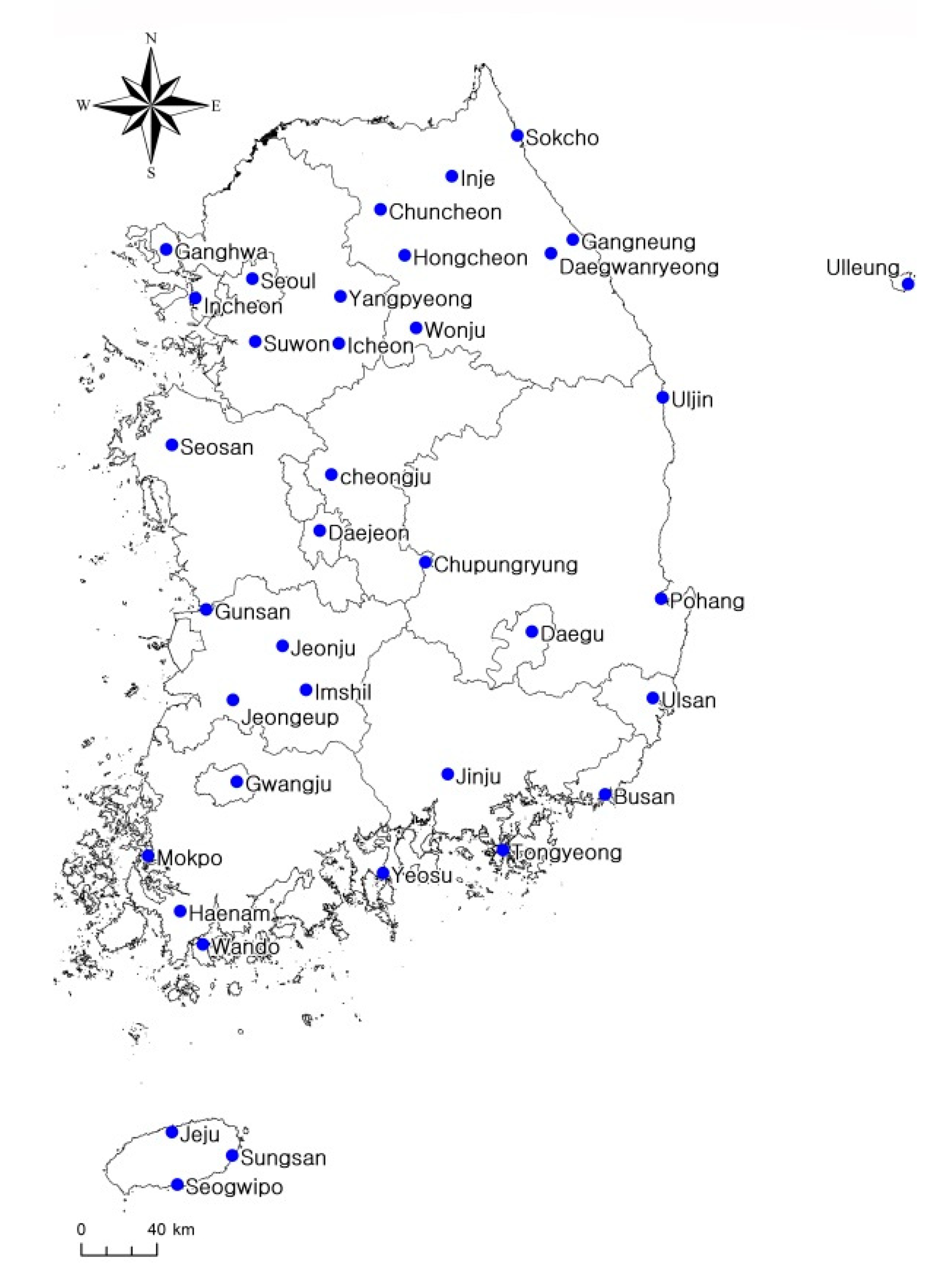
The hydrological time series data used for the analysis required testing. However, in the case of the data from South Korea, the test results showed a low confidence interval because of the short observation period. Therefore, in this study, data were collected for each of the 37 stations located across the country that began recording observations in 1971. These stations recorded data for at least 45 years, and the characteristics of annual precipitation time series data were assessed. Figure 2 shows the locations of the 37 stations selected for this study.
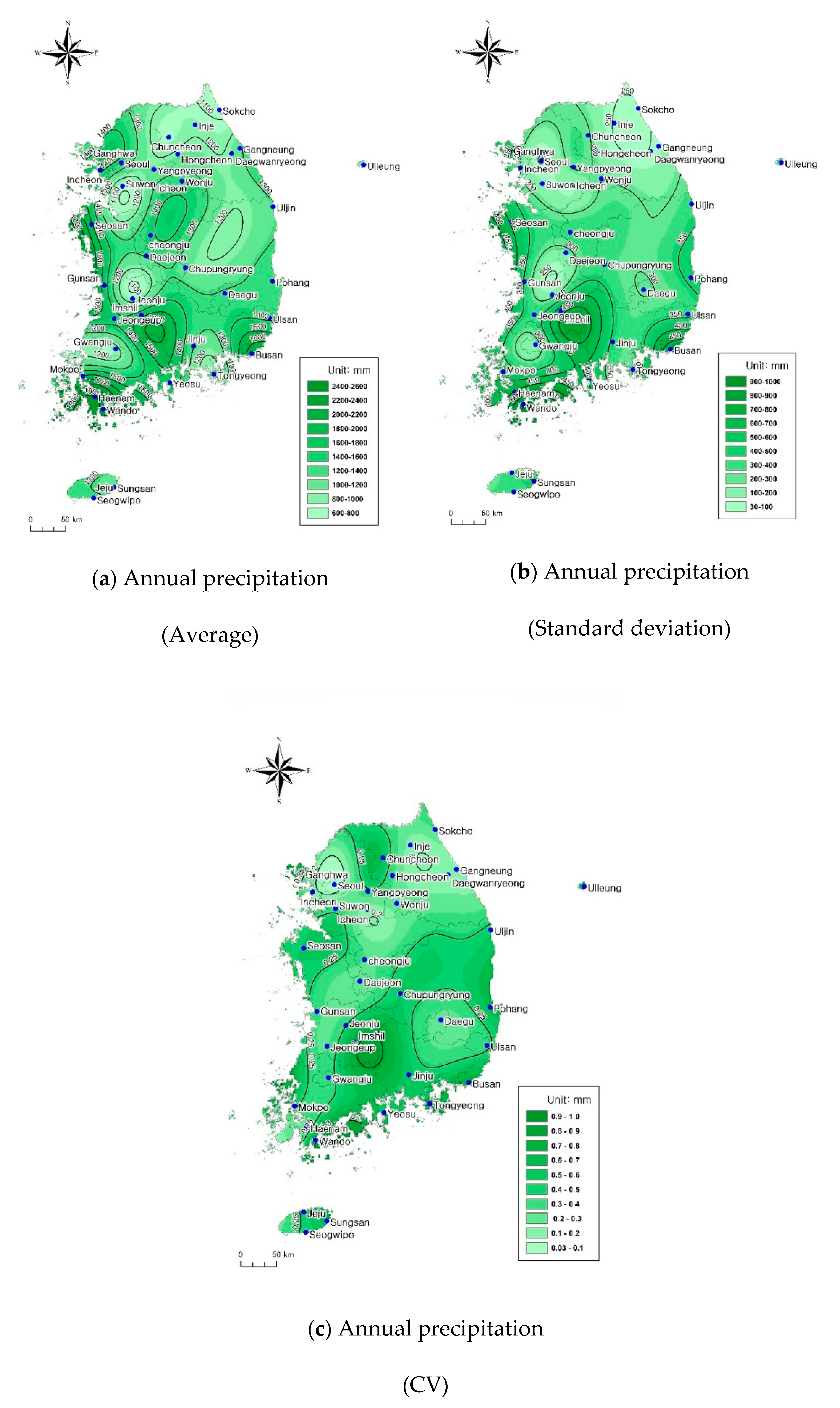
To identify the trends with regard to changes in annual precipitation for South Korea, we analyzed the characteristics of the time series for the 37 weather stations taking into account the spatial distribution of the annual precipitation averages and standard deviations of the data from these stations. The annual precipitation average was highest for the Jeju area (1905 mm/year for Seogwipo and 1850 mm/year for Seongsan) and lowest for the Daegu station (1052 mm/year). In addition, the study calculated the CVs to evaluate the variability in annual precipitation. The CVs were obtained by dividing the standard deviation by the numerical mean. A low CV indicated that the annual data had low variability and high stability. The annual precipitation CV was found to be lowest for the Sokcho station and highest for the Seongsan station, indicating that the annual precipitation data of the Sokcho station was stable and least variable while that of the Seongsan station was unstable and highly variable. Figure 3 shows the spatial distribution of averages, standard deviations, and CVs of the annual precipitation data in this study.

2.2.2. Climate Change Scenarios

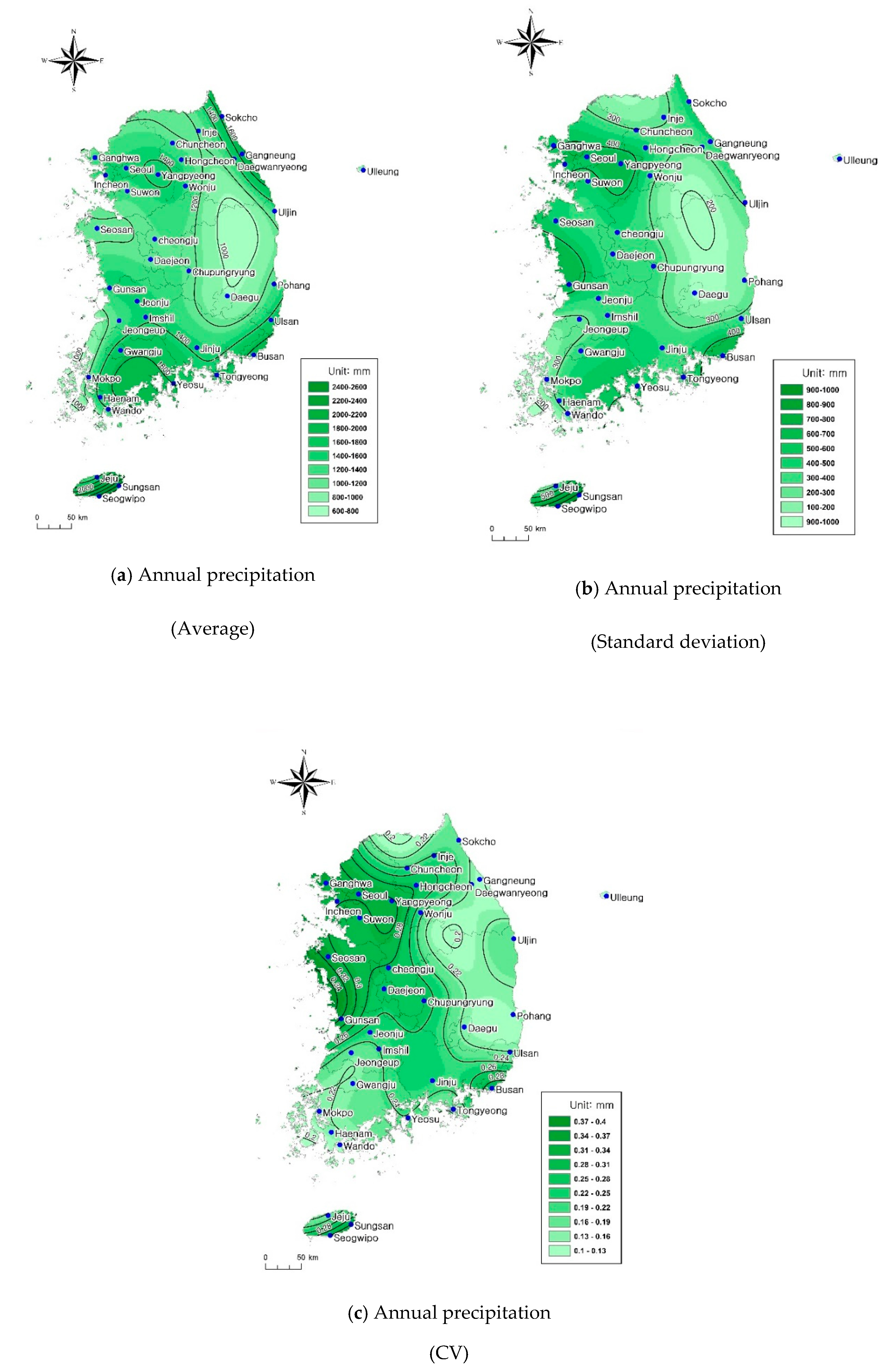
The GCM, a numerical climate model, has several types and produces different simulation results depending on the type of input data used. Meteorological data predicted by the GCM are statistically downscaled for practical use. The KMA operates a certification system to encourage the use of diverse scenarios. The system recommends 13 scenarios at a regional level that are produced with the combination of GCMs scenarios and statistical down-scaling (Table 1). For such statistical downscaling, SDQDM has been recommended as it was designed to preserve the long-term trends of climate models and conducts a bias correction [16]. In this study, 13 regional scale scenarios produced by SDQDM, a statistically detailed technique, were used with the GCM scenarios provided by the Standard Scenario Certification System of the Korea Meteorological Administration. Figure 4 shows the climate change scenarios. Figure 5 shows the spatial distribution of averages, standard deviations, and CVs of the future annual precipitation data in this study. The results showed that the annual precipitation average will be highest for the Seogwipo station (2445 mm/year) and lowest for the Daegu station (1023 mm/year). The standard deviation was the highest in Seogwipo (733), the lowest in Ulleung (201), the highest in CV (Gunsan (0.32)), and the lowest in Pohang (0.21).

2.2.3. Performance of Climate Change Scenarios

To verify the performance of MME from the 13 climate change scenarios of GCMs, the study draws a box plot, using spatially calculated averages for monthly precipitation and mean temperature data provided by 80 weather stations for the reference period for each of the models. In addition, the coefficient of variation (CV) between models was calculated by station point for annual precipitation and average temperatures of the late 21st century (2071–2100).
The study statistically down-scaled the 13 national standard scenarios, using the SDQDM of the AIMS provided by the Asia Pacific Economic Cooperation Climate Center (APCC). In this chapter, the study compares probability density functions (PDFs) and spatial distribution between MME, (precipitation and temperature), which is down-scaled for the period of reference climate, and observation data. This aims to verify the applicability of statistical down-scaling results, for North Korea’s climate observation.
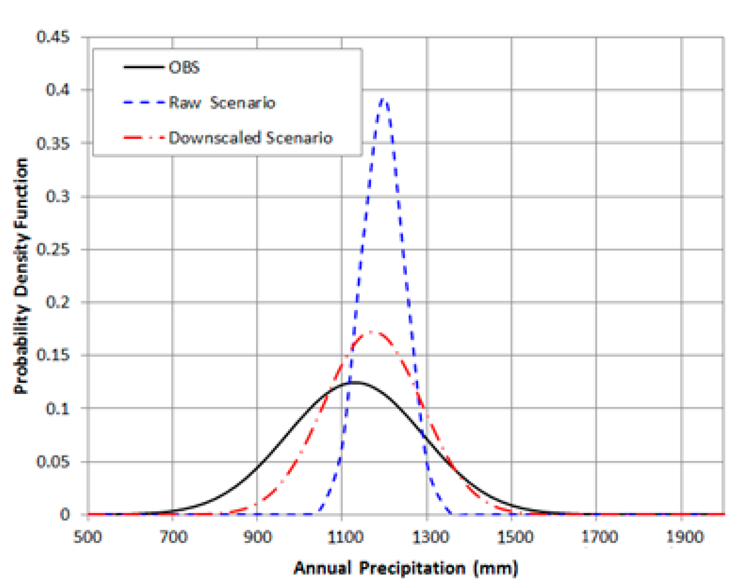
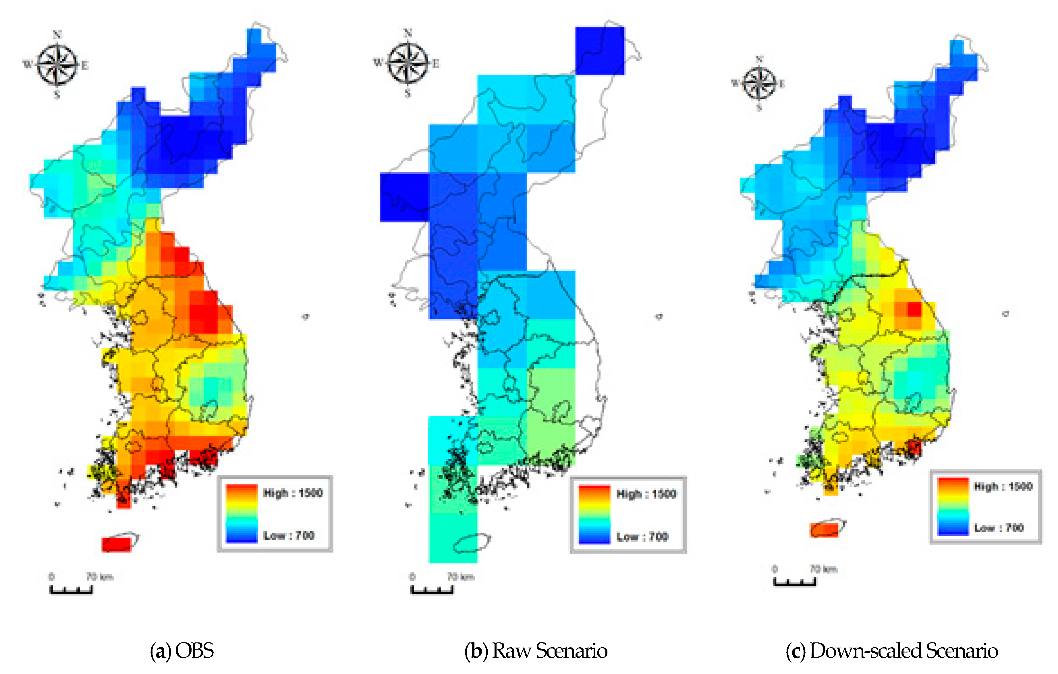
For annual precipitation, the PDFs were compared between the observation data and before application or after application of the SDQDM. This is well matched to the bell-shaped, normal distribution for the average value, while variables were gathered around the median. Comparing average values (mode and median) and variances between before down-scaling (blue line in Figure 6), and after down-scaling (red line in Figure 6), the study found that they were well matched to those of observation data after down-scaling. For quantitative results, the average value of OBS is 1116 mm, the average of the raw scenario is 1196, the average of the downscaled scenario is 1162 mm, and it is confirmed that the observation and the after down-scaling are similar. The result of comparing spatial distribution between before/after down-scaling suggested that the latter simulated the spatial distribution very close (Figure 7a,c) to that of observation data (Figure 7a).

3. Evaluation of Time Series Characteristics Using Observational Data of Precipitation

3.1. Hydrological Persistence Test

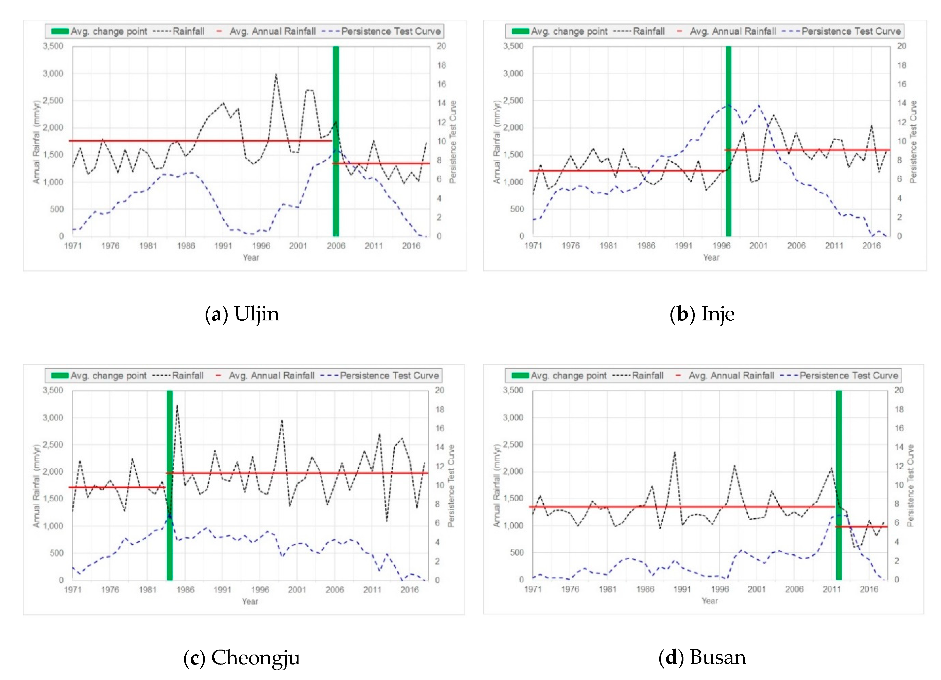
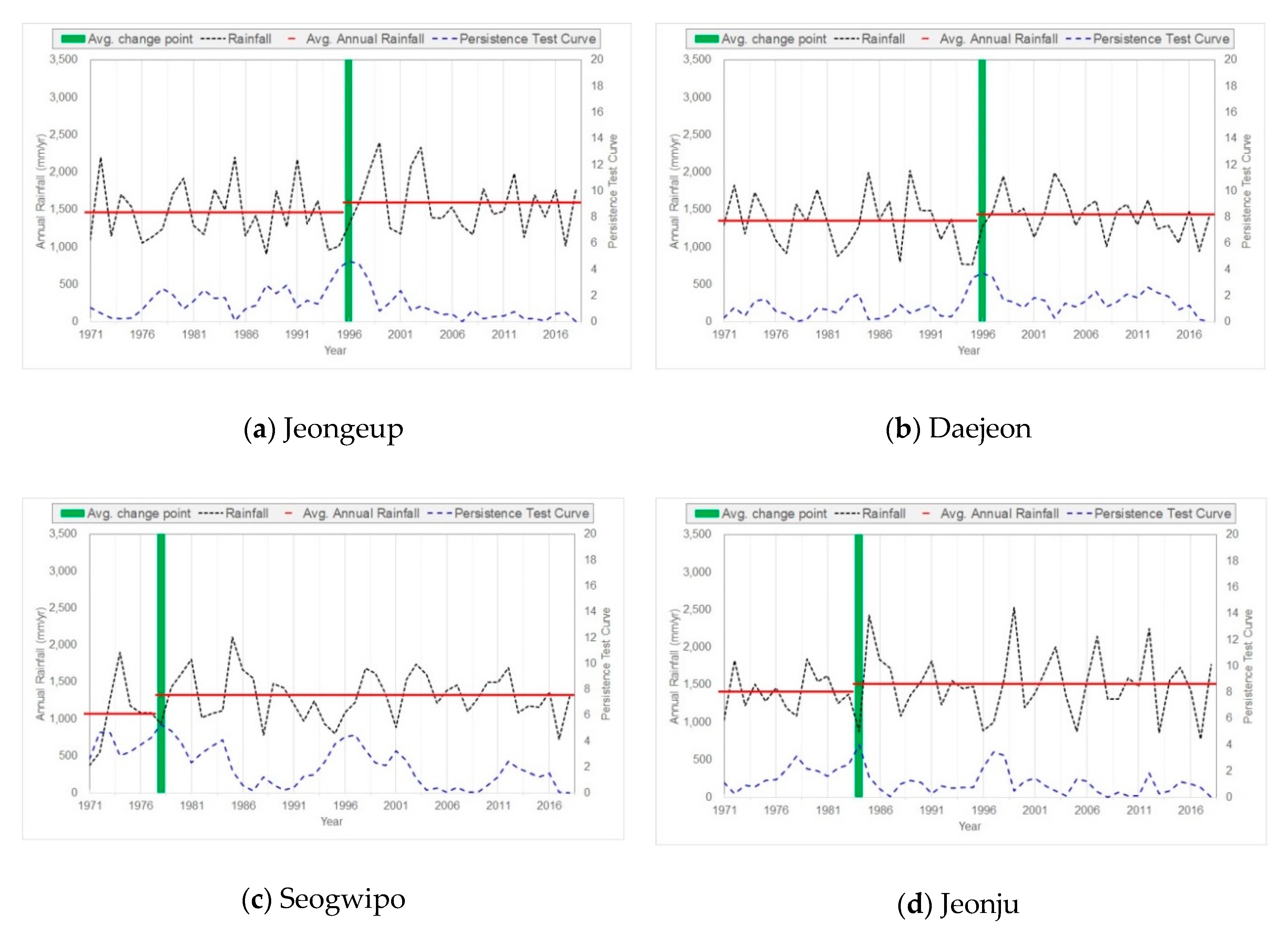
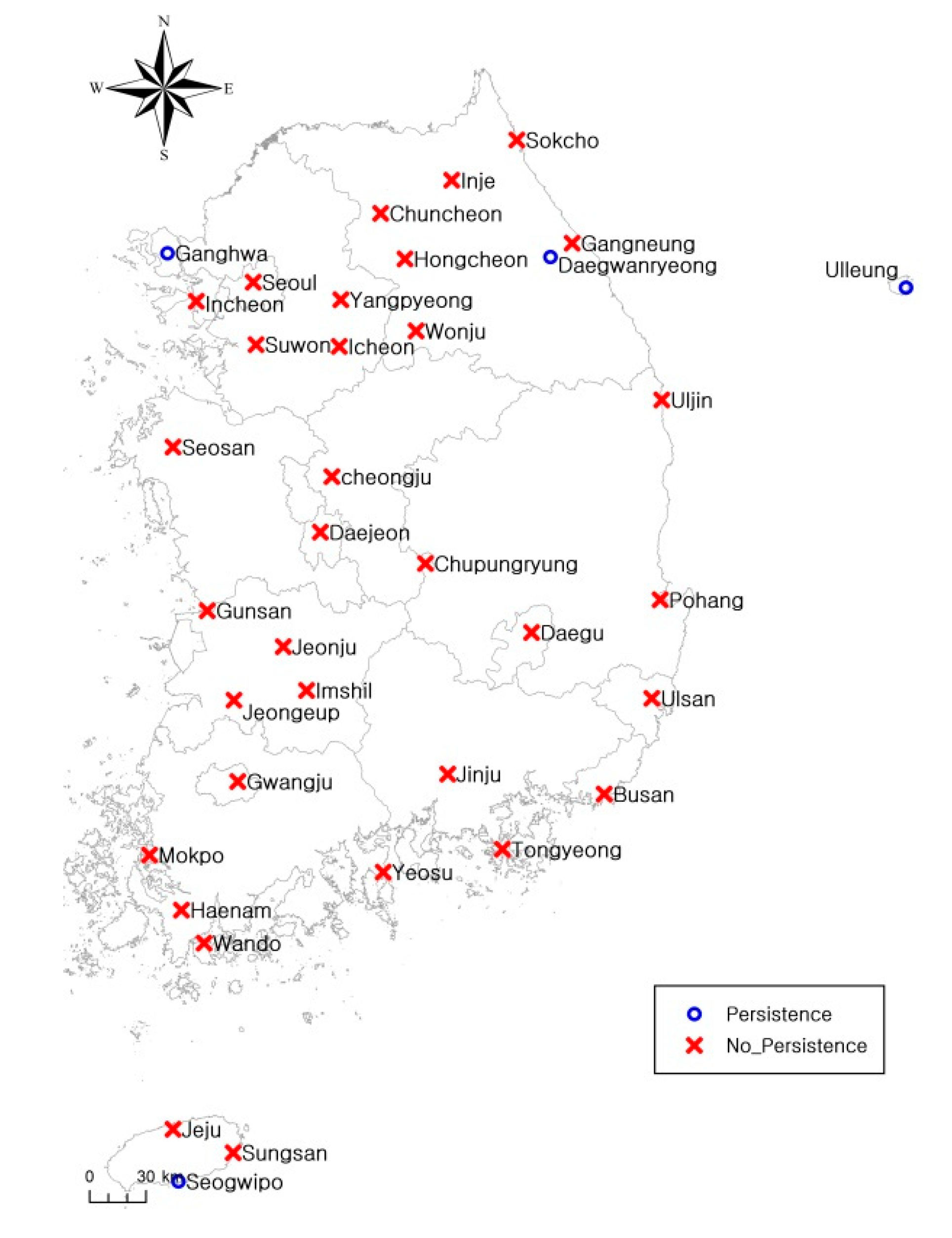
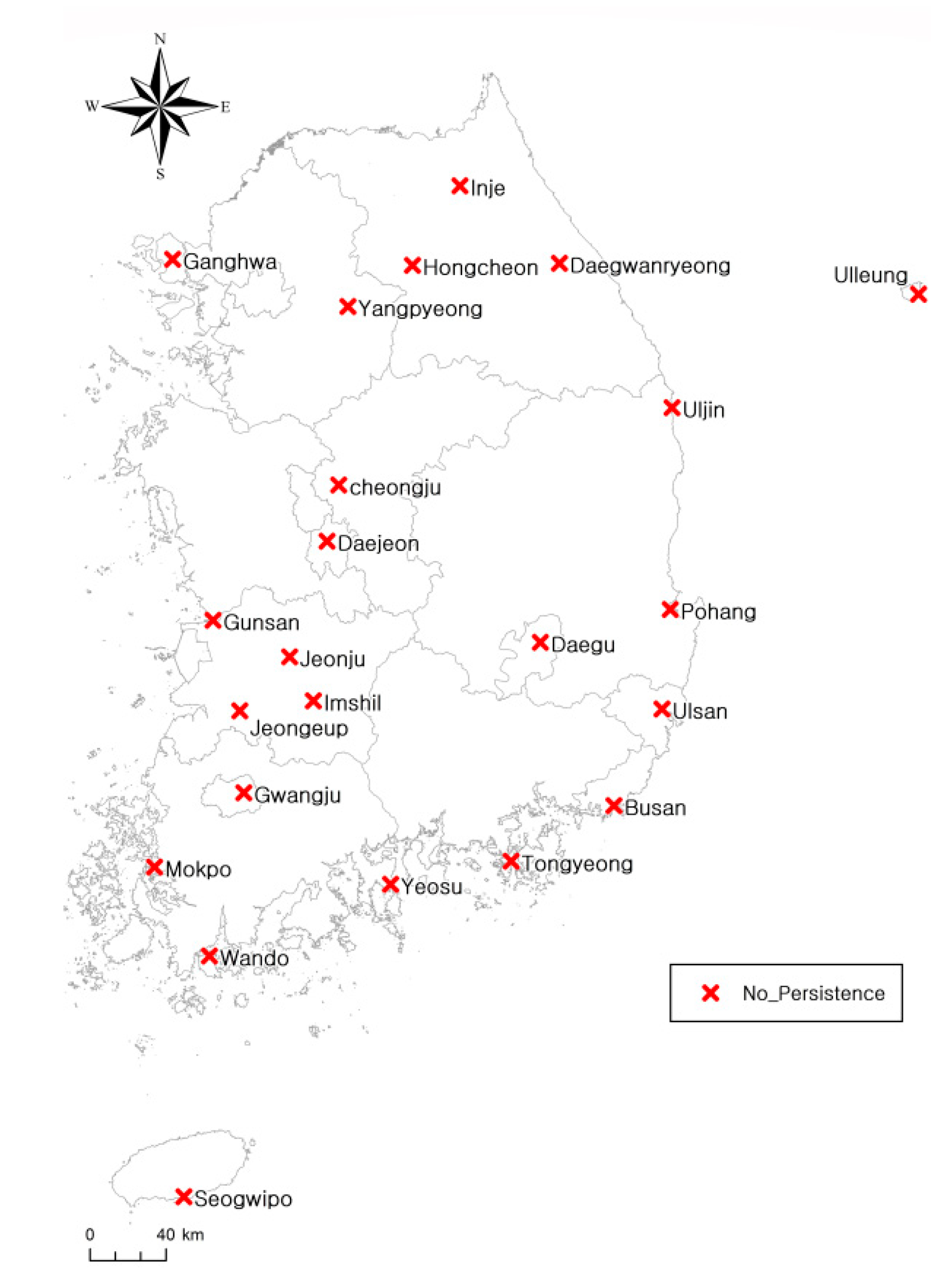
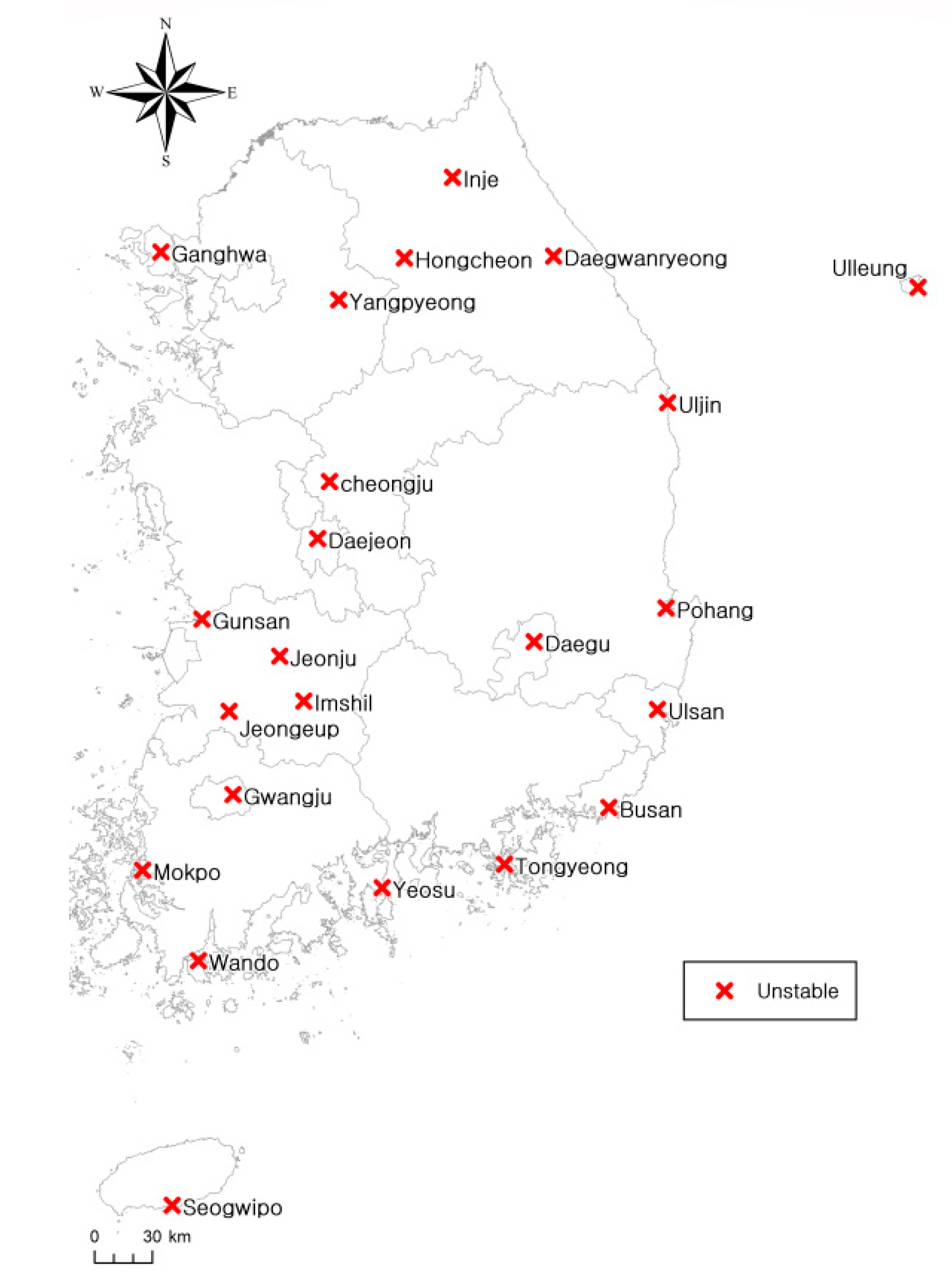
A persistence test was conducted using the cumulative deviation to evaluate annual precipitation data. When persistence exists, data averages show inconsistency and randomness. Therefore, persistence in data is indicative of nonstationarity. After evaluating persistence using a cumulative deviation analysis, one station showed increasing annual precipitation since 1978. Out of the 37 selected stations, 19 and 17 stations showed increasing trends in annual precipitation from 1982 to 1989 and from 1994 to 1997, respectively. The study also used the serial correlation coefficient to evaluate persistence. In a previous study, persistence was only explained for the Daegwallyeong station [13]. However, the results of this study suggested that four stations (i.e., Daegwallyeong, Ulleung, Seogwipo, and Ganhwa) showed persistence, as summarized in Table 2. In addition, the graphs of Figure 8 and Figure 9 show the results of the persistence analysis using the serial correlation coefficient. Each graph shows an inflection point, annual precipitation, the averages before and after the inflection point, and a standardized cumulative value of annual precipitation. The graphs in Figure 8 show the persistence analysis results for the Daegwallyeong, Ulleung, Seogwipo, and Ganhwa stations. In contrast, the graphs in Figure 9 show the results for the Busan, Gwanju, Haenam, and Jeju stations, which did not show persistence. The map shown in Figure 10 indicates the stations with and without persistence.

3.2. Hydrological Trend Test

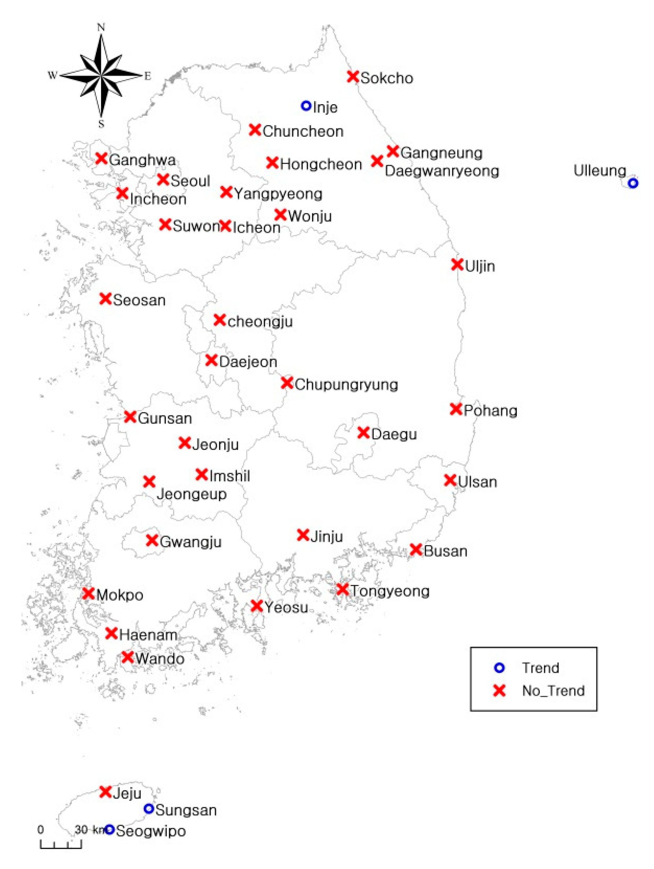
To evaluate the annual precipitation data, we used the Spearman rank correlation test to analyze possible trends. This study also conducted a two-tailed statistical test with significance at the 5% level for each of the dataset. An increasing or decreasing trend with regard to the average and variance may be present in a time series. Therefore, when the statistical characteristics such as average and variance are constant with time, the data cannot be considered stationary. Therefore, when statistics, such as the average and variance, are constant over time, the data are considered to show stationarity. Table 3 shows the results of the Spearman rank correlation analysis. Out of the 37 stations, the annual precipitation data from the Uleungdo, Seongsan, Seogwipo, and Inje stations showed increasing trends with variations between stations. Among the four stations, Seongsan station showed the greatest trend. In a past study [13], data from 1972 to 1995 were used to analyze the trends of Daegwallyeong station. However, in this study, no trend was observed for this station as the decrease in annual precipitation since 1994 was offset by the current increasing trend. The map in Figure 11 shows the results of the trend analysis.

3.3. Hydrological Stable Test

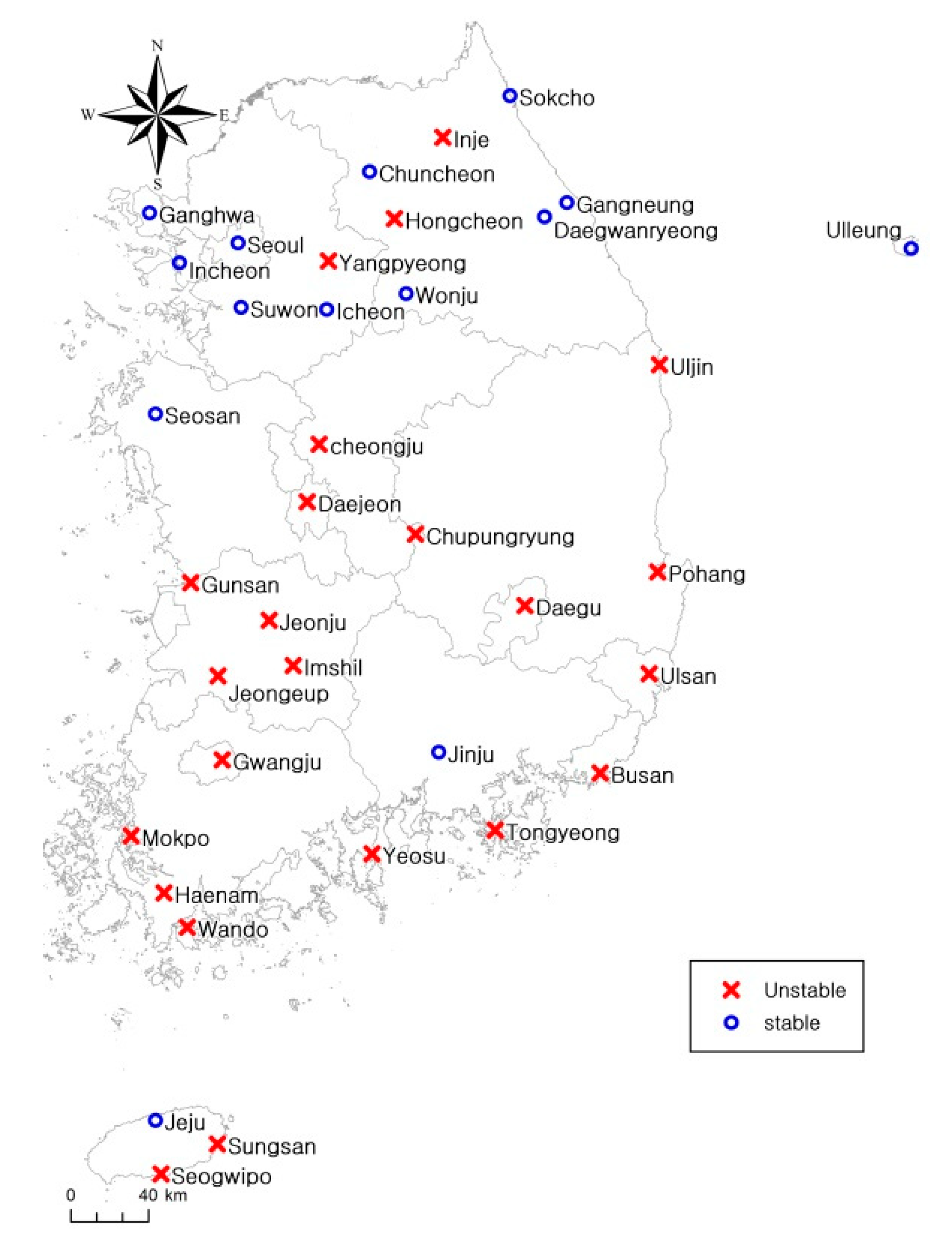
A simple T-test and F-test were used to test the stability of annual precipitation. Two-tailed tests with significance at the 5% level were conducted for each dataset. The data in which statistics, such as the average and variance, were not consistent were considered nonstationary. Table 4 summarizes the simple T-test and F-test results. For the simple T-test, 23 of the 37 stations showed unstable annual precipitation, including the Uljin, Cheongju, Daejeon, Chupungnyeong, Pohang, Gunsan, Daegu, Jeonju, Busan, and Ulsan stations. The simple F-test results show that the annual precipitation data from two stations, Seongsan and Haenam, were unstable. According to [13], out of the stations that showed unstable data, the Uljin, Cheongju, Daejeon, and Chupungnyeong stations showed the greatest changes in trends, and data from the Daegwallyeong, Ganghwa, and Imsil stations were found to be stable. However, in this study, data from all stations, except Imsil, were unstable, whereas the data from 23 stations, including Uljin, Cheongju, and Imsil, were analyzed for instability. Figure 12 shows the simple T-test and F-test results.

3.4. Estimation of Hydrological Stationarity

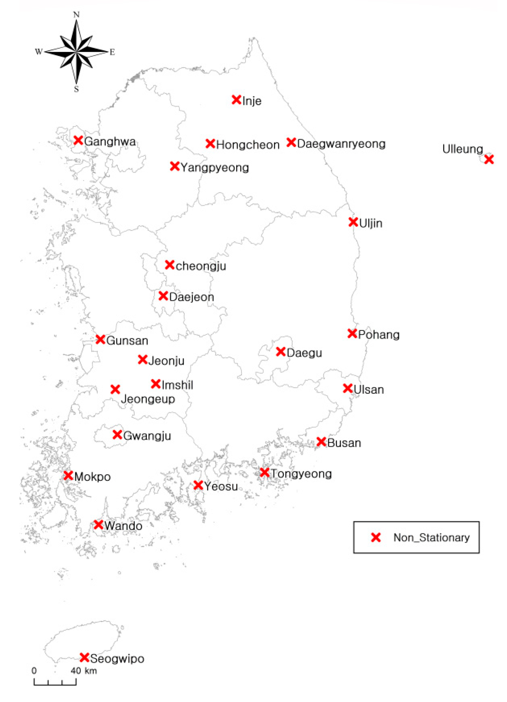
As shown in Table 5, data from the 14 stations that showed stability without trends or persistence were deemed to show stationarity. The data from 23 stations that showed abnormality in two out of the three features (i.e., persistence, trends, and stability) were deemed nonstationary. According to [13], data from the Daegwallyeong, Uleungdo, Yangpyeong, and Jecheon stations showed nonstationarity. However, in this study, we found that the data from 23 stations, including Uleungdo station, showed nonstationarity. Moreover, the data from Daegwallyeong station were considered to show stationarity. Figure 13 shows the results of the stationarity analysis for the annual precipitation data of the 37 stations.

4. Prediction of Changes in Time Series Characteristics with Climate Change Scenarios

4.1. Selected Stations

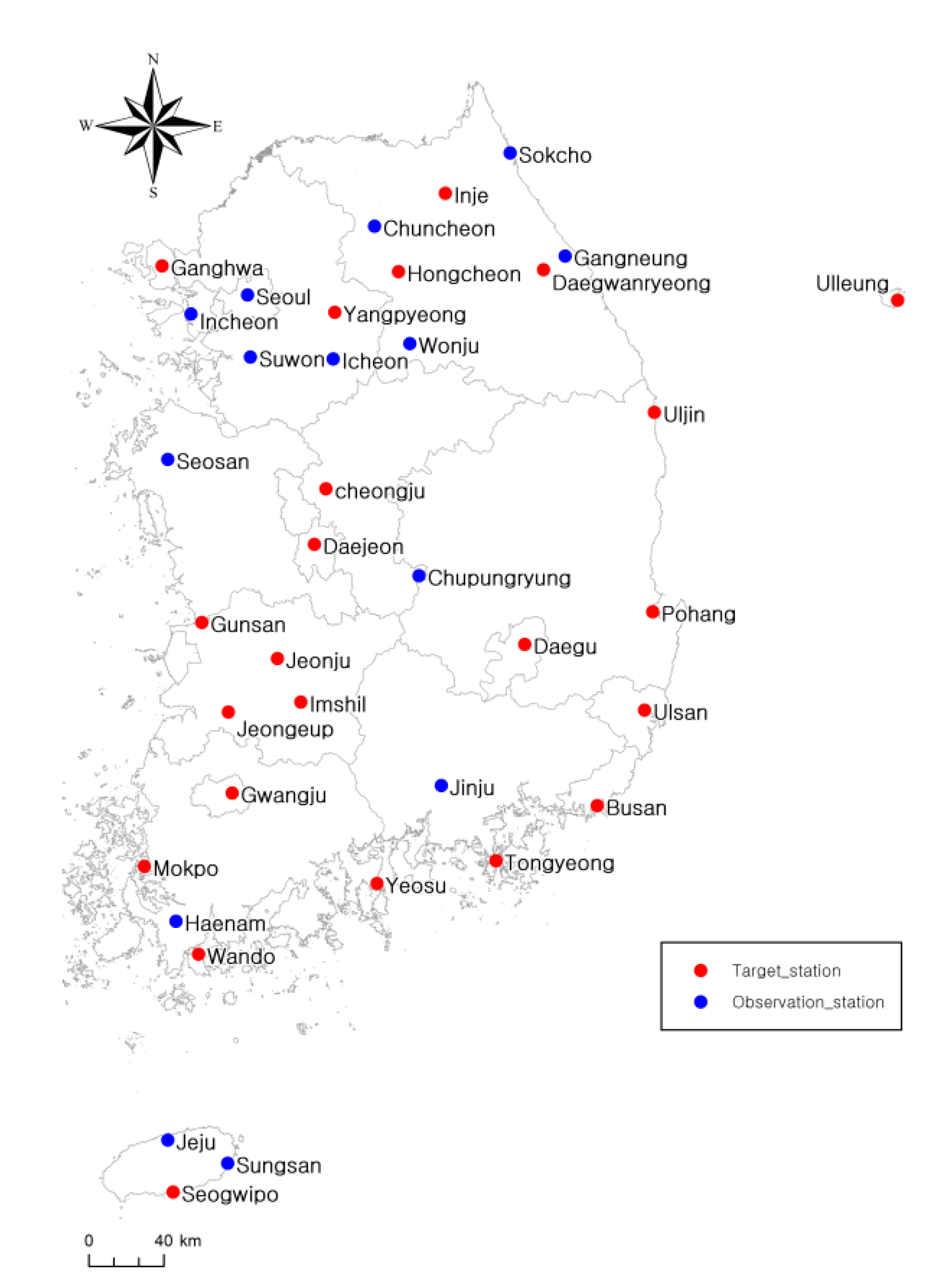
We selected 25 stations that showed nonstationarity based on the results of the stationarity analysis using current annual precipitation data. With the exception of Chupungnyeong and Seongsan stations, for which climate change scenarios were not available, all stations were used for the stationary analysis using future annual precipitation scenarios for South Korea with SDQDM, a statistical downscaling model. Figure 14 shows the spatial distribution of the observations for this study. The blue dot is the entire station, and the red dot is the station analyzed using climate change scenario data.

4.2. Hydrological Persistence Test Using Climate Change Scenarios

To determine the hydrological persistence of future annual precipitation data, we used a persistence analysis with the cumulative deviations and serial-correlation coefficients of future annual precipitation data of the 23 aforementioned stations. [13] suggested that persistence was only present for Daegwallyeong station. However, in this study, the analysis of the current annual precipitation indicated the presence of persistence in the Jeongeup, Uleungdo, Seogwipo, and Seongsan stations, whereas the analysis using climate change scenarios suggested that this feature did not appear in any station. Figure 15 shows the cumulative graphs of the stations for which the data did not show persistence, namely the Jeongeup, Daejeong, Seogwipo, and Jeonju stations. Table 6 summarizes the results of the serial correlation coefficient analysis, and Figure 16 shows the results of the persistence analysis.

4.3. Hydrological Trend Test Using Climate Change Scenarios

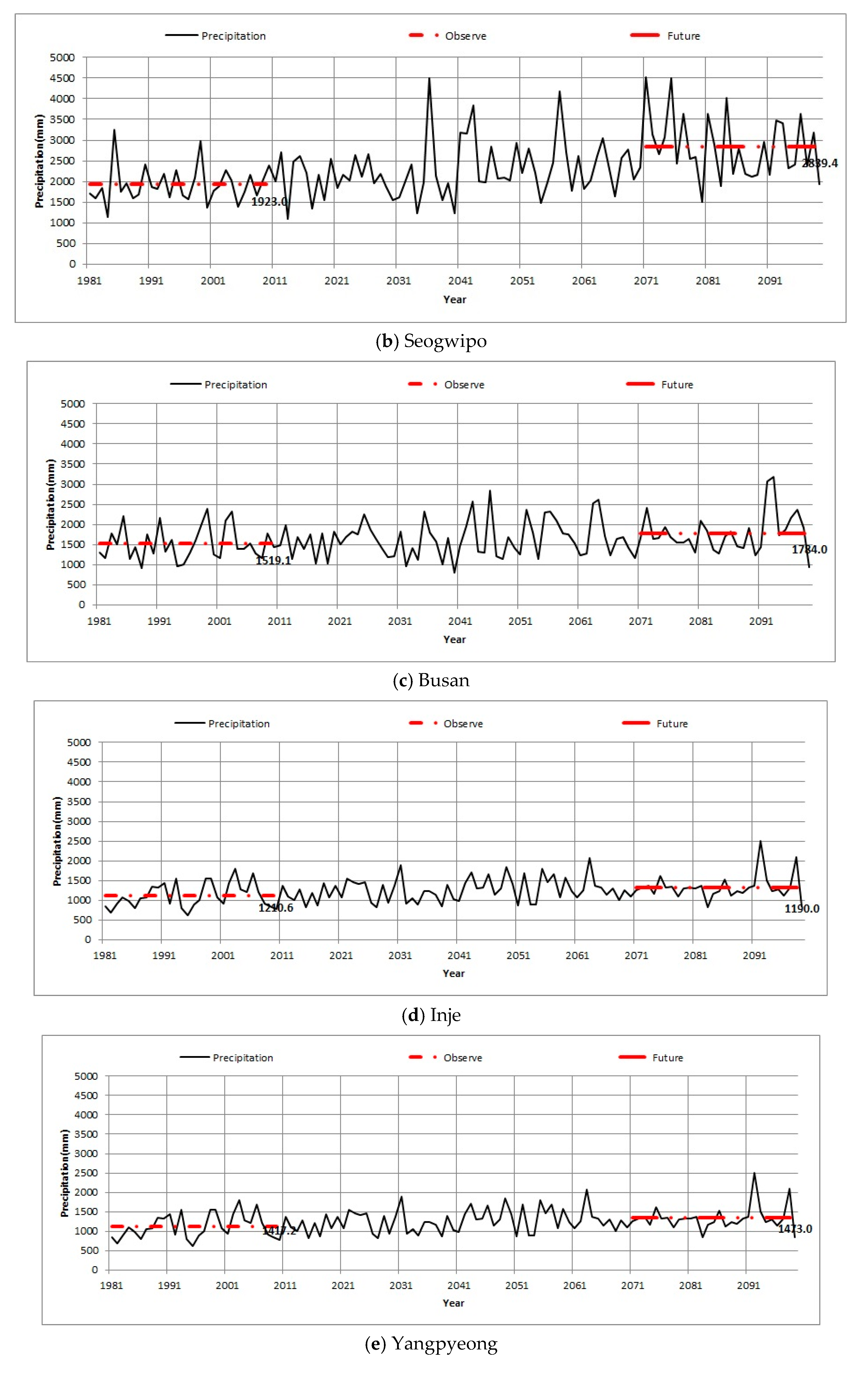
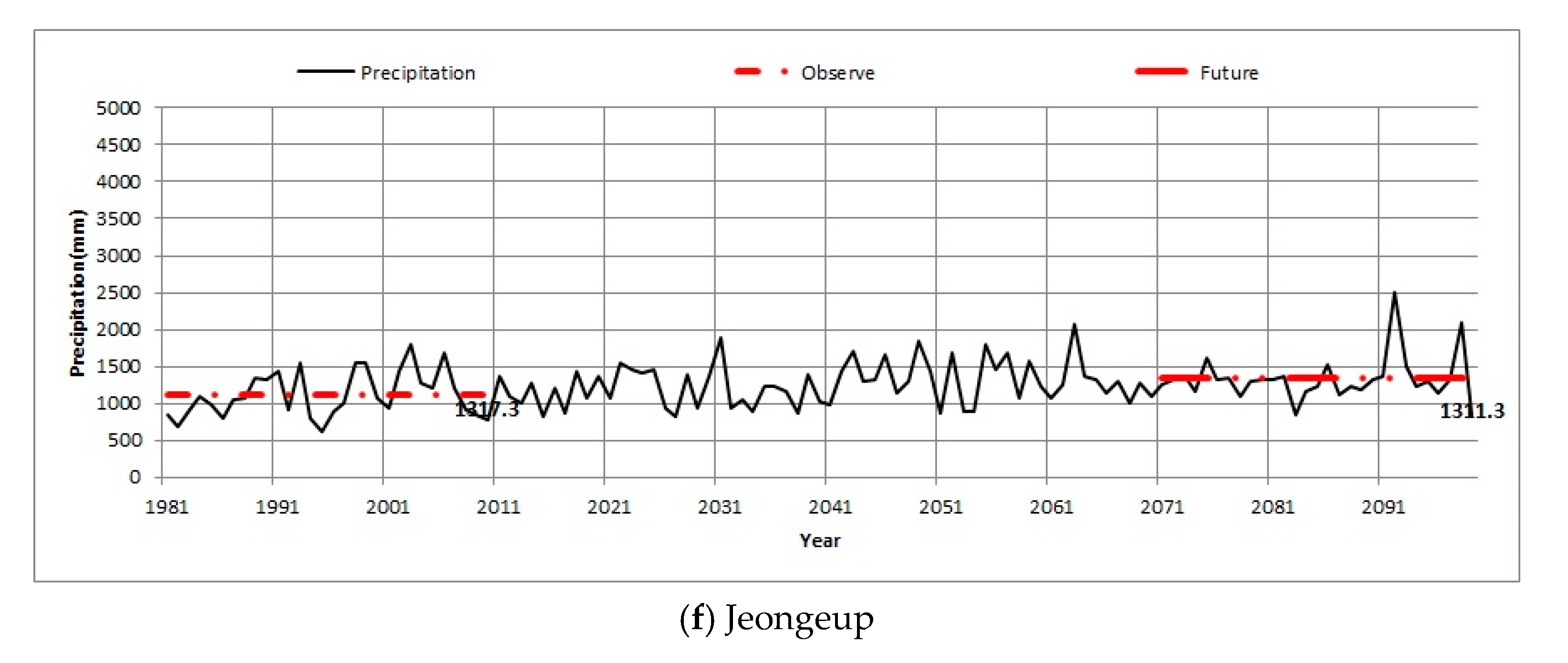
This study used a Spearman rank correlation analysis to analyze trends in annual precipitation using climate change scenarios. A two-tailed statistical test with significance at the 5% level was used for each dataset. Table 6 shows the trends in annual precipitation data for 11 out of the 23 stations, including the Busan, Seogwipo, Yangpyeong, and Jeongeup stations. In a previous study [13], data from 1972 to 1995 was used to analyze the trends of Daegwallyeong station. However, in this study, the analysis of this data indicated no significant trend for this station as the decrease in the annual precipitation since 1995 was offset by the current increasing trend. A comparison between the current data and that of the Future 3 scenario (2071 to 2100), the latter of the climate change scenarios, indicated that Seogwipo station showed the highest rate of increase (28.7%). The lowest rate of decrease was present at Daegu station (10.1%). In addition, Busan and Yangpyeong stations showed increasing trends of 8.6% and 3.8%, respectively. In addition, Uljin and Inje stations showed decreasing trends of 1.3% and 2.3%, respectively. These results suggest that variations in the trends of annual precipitation of the target stations. The results of the trend analysis are summarized in Table 7, while Figure 17 provides the graphs of six stations and depicts changes in current and future annual precipitation. Figure 18 shows the results of the trend analysis.

4.4. Hydrological Stability Analysis Using the Climate Change Scenarios

For the annual precipitation stability analysis using climate change scenarios (2011–2099), we used simple T-test and F-test analyses. With the results, we used a two-tailed test with significance at the 5% level for each data. Table 8 shows the Simple T-test and F-test results. The Uljin, Busan, Seogwipo, Yangpyeong, Inje, and Jeongeup stations showed instability. [13] indicated that the data showed instability for the Daegwallyeong, Ganghwa, and Imsil stations. In this study, the results suggested that the data were unstable for all 21 stations (Table 7), which was also supported by the simple T-test and F-test results. Figure 19 shows the results of the stability test.

4.5. Estimation of Hydrological Stationarity Using Climate Change Scenarios

We analyzed persistence, trends, and stability to determine the stationarity of annual precipitation data based on climate change scenarios. The results are summarized in Table 9 for the 23 stations that showed nonstationary with current data, including the Daegwallyeong, Uleungdo, Yangpyeon, and Jecheon stations. However, the analysis of future data found that nonstationary was present in 23 stations, including those of the current study. Figure 20 shows the results of the stationarity analysis.

5. Conclusions

The study collected annual precipitation data from 37 weather stations across Korea that had collected data for 45 years or longer with the aim to analyze the stationarity of the data. We also conducted persistence, trend, and stability analyses and then screened out stations that showed nonstationarity of annual precipitation data. For the remaining stations, we used climate change scenarios and analyzed the stationarity of future annual precipitation data. The results can be summarized as follows.
(1) After analyzing the persistence of data from 37 stations, annual precipitation at Haenam station was found to have increased since 1978. In addition, 19 stations, including Gangneung, Ulsan, Jeonju, Ganghwa, and Seongsan, showed increasing precipitation trends from 1982 to 1989, whereas 17 stations, including Chupungnyeong, Daejeon, Gunsan, Chuncheon, Uleungdo, and Gwangju, showed increasing precipitation trends from 1994 to 1997. Stationarity was observed in four stations: Daegwallyeo, Uleungdo, Seogwipo, and Ganghwa.
(2) The trend analysis for the annual precipitation of the target stations suggested that no trends were present for most regions. However, the Uleungdo, Seongsan, Seogwipo, and Inje stations showed some evidence of trends. Among these, Seongsan station showed the distinct trend of increasing annual precipitation.
(3) The stability analysis of 23 stations, including that of the Uljin, Cheongju, Daejeon, and Chupungnyeong stations, showed that the annual precipitation data was unstable. In particular, the Seogwipo station registered the highest annual precipitation (more than 2000 mm) from 2009 to 2012 and 2014 to 2016. Therefore, it can be concluded that the influence of such periods caused data instability.
(4) Based on the results of the persistence, trend, and stability analyses, stationarity was detected. In particular, 14 stations showed stationarity, whereas 25 stations showed nonstationarity. The stations with nonstationarity accounted for 67% of all stations. Most of the stations in the central region, except the Inje, Hongcheon, and Yangpyeong stations, and most of the stations in the southern region, except the Jinju and Jeju stations, showed stationarity. The principle reason for the nonstationarity of these stations in the southern region was the influence of typhoons that led to persistence and instability in the annual precipitation data.
(5) The stationarity analysis for future annual precipitation using climate change scenarios showed that out of 23 stations, 12 stations showed trends, 23 stations had unstable data, and no station showed persistence as climate change caused changes in annual precipitation characteristics. Therefore, future hydrological analysis should consider the influence of climate change on the characteristics of hydrological time series.
In addition, the results obtained were different from those of a previous study [13], wherein nonstationarity was observed for multiple stations, including Daegwallyeong, Uleungdo, Yangpyeong, and Jecheon. However, in this study, 25 stations, including Uleungdo, showed nonstationarity. Moreover, the results of the stationarity analysis of future annual precipitation using climate change scenarios suggests that climate change will influence the characteristics of hydrological time series data. For example, the stations that showed a trend in the present also showed persistence without the trend. This underlines the necessity of reconsidering present hydrological analyses with the variable characteristics of annual precipitation. Therefore, in hydrological analyses that use annual precipitation in South Korea, nonstationarity needs to be considered beyond the current assumption of stationarity. In addition, current analyses should be reviewed by considering the current characteristics of annual precipitation and the influence of climate change on future annual precipitation. Moreover, it is also necessary to statistically identify climate characteristics in diverse conditions by analyzing the correlations among a range of hydro-meteorological factors with regard to annual precipitation in the future as time series characteristics with respect to trends, stability, and persistence are likely to be affected by climate change. Furthermore, the results of this study are expected to contribute to long-term plans regarding the preventive management measures that must be undertaken with regard to natural phenomena, including those for flooding, as well as additional studies that are conducted on time series that consider the influence of climate change on diverse hydro-meteorological factors.

Author Contributions

Investigation, B.-H.L.; Writing—original draft, G.-K.L.; Writing—review & editing, B.-S.K. and S.-J.J. All authors have read and agreed to the published version of the manuscript.

Funding

This work was funded by the Korea Meteorological Administration Research and Development Program under Grant KMI [2018-03010]. This study was supported by a 2017 research grant from Kangwon National University [number 620170154].

Acknowledgments

The authors express their sincere thanks to the Korea Meteorological Administration and Kangwon National University.

Conflicts of Interest

The authors declare no conflict of interest. The funders had no role in the design of the study; in the collection, analyses, or interpretation of data; in the writing of the manuscript, or in the decision to publish the results.

References

  1. Oh, J.S.; Seo, B.H.; Kim, H.S. Trend and shift analysis for hydrologic and climate series. KSCE J. Civ. Eng. 2006, 26, 355–362. [Google Scholar]
  2. Vaskar, D.; Sudip, G.I.D.; Rabin, B. Analysis of the long-term precipitation trend in Illinois and its implications for agricultural production. Water 2018, 10, 433. [Google Scholar]
  3. Park, J.H.; Lee, G.S.; Yang, J.S.; Kim, S.W. A hydrometeorological time series analysis of Geum River watershed with GIS data considering climate change. J. Korea Spat. Inf. Soc. 2012, 20, 39–50. [Google Scholar] [CrossRef] [Green Version]
  4. Lee, J.J.; Jang, J.Y.; Kwak, C.J. An analysis of temporal characteristic change for various hydrologic weather parameters (I)—On the basic statistic, trend. J. Korea Water Resour. Assoc. 2010, 43, 409–419. [Google Scholar] [CrossRef] [Green Version]
  5. Rawshan, A.; Alban, K.; Shadan, A.; Ozgur, K. Long-term trends and seasonality detection of the observe flowin Yangtze River using mann-kendall and sen’s innovative trend method. Water 2019, 11, 1855. [Google Scholar]
  6. Ryu, Y.; Shin, H.; Kim, S.; Heo, J. Power test of trend analysis using simulation experiment. J. Korea Water Resour. Assoc. 2013, 46, 219–227. [Google Scholar] [CrossRef] [Green Version]
  7. Kim, T.R.; Shin, H.J.; Joo, K.W.; Heo, J.H. Trend analysis of extreme hydrological data considering skewness degree. KSCE J. Civ. Eng. 2013, 10, 1771–1773. [Google Scholar]
  8. Kang, B.S.; Lee, S.C.; Kwon, J.W. Analysis of climate change characteristics of hydrologic data on the Korean Peninsula through normality and homogeneity Tests: Properties analysis of climate change on hydrologic variance in Korea using Stationary and homogeneity test. In Proceedings of the 2009 Conference of Korean Society of Civil Engineers, Seoul, Korea, 21 October 2009; pp. 2534–2537. [Google Scholar]
  9. So, B.J.; Kwon, H.H.; An, J.H. Trend analysis of extreme precipitation using quantile regression. J. Korea Water Resour. Assoc. 2012, 45, 815–826. [Google Scholar] [CrossRef] [Green Version]
  10. Kim, J.; Kim, S.; Park, M.; Joo, J. A comparison of drought prospection by future climate models. J. Korean Soc. Hazard. Mitig. 2016, 16, 463–472. [Google Scholar] [CrossRef] [Green Version]
  11. Sung, J.H.; Kim, B.; Kang, H.S.; Cho, C. Non-stationary frequency analysis for extreme precipitation based on representative concentration pathways (RCP) climate change scenarios. J. Korean Soc. Hazard. Mitig. 2012, 12, 231–244. [Google Scholar] [CrossRef] [Green Version]
  12. Ahn, J.; Choi, Y.W.; Jo, S.; Hong, J.Y. Projection of 21st century climate over Korean Peninsula: Temperature and precipitation simulated by WRFV3.4 Based on RCP4.5 and 8.5 scenarios. J. Korean Meteor. Soc. Atmos. 2014, 24, 541–554. [Google Scholar] [CrossRef] [Green Version]
  13. Kim, B.S.; Kang, K.S.; Seo, B.H. The time series analysis of annual precipitation in Korea. In Proceedings of the 1997 Conference of Korea Water Resources Association, Seoul, Korea, 5 May 1997; pp. 280–285. [Google Scholar]
  14. Dahamen, E.R.; Hall, M.J. Screening of Hydrological Data: Tests for Stationary and Relative Consistency; International Institute for Land Reclamation and Improvement: Wageningen, The Netherlands, 1990. [Google Scholar]
  15. Jung, S.J. Impact Assessments of Climate and Hydrological Cycle Changes in North Korea Based on RCP Climate Change Scenarios. Ph.D Thesis, Kangwon National University, Chuncheon, Korea, 2019. [Google Scholar]
  16. Jeung, S.J.; Sung, J.H.; Kim, B.S. Assessment of the impacts of climate change on climatic zones over the Korean Peninsula. Adv. Meteorol. 2019, 2019, 1–11. [Google Scholar] [CrossRef] [Green Version]
Figure 1. Flow chart of Stationary test.
Atmosphere 11 01027 g001
Figure 2. Stations for the study.
Atmosphere 11 01027 g002
Figure 3. Average, coefficient of variation (CV), and standard deviation of the annual precipitation (mm). (a) is the average of the annual precipitation, (b) is the standard deviation of the annual precipitation, and (c) is the CV value of the annual precipitation.
Atmosphere 11 01027 g003
Figure 4. Climate Change Scenarios Used in This Study.
Atmosphere 11 01027 g004
Figure 5. Average, coefficient of variation (CV), and standard deviation of annual precipitation (mm) using the climate change scenarios. (a) is the average of the annual precipitation, (b) is the standard deviation of the annual precipitation, and (c) is the CV value of the annual precipitation.
Atmosphere 11 01027 g005
Figure 6. Observation and probability density functions of before/after application of the spatial disaggregation with quantile delta mapping (SDQDM) (annual precipitation).
Atmosphere 11 01027 g006
Figure 7. Spatial distribution for observation and before/after down-scaling (annual precipitation). (a), (b), and (c) represent OBS, Raw-Scenario, and Down-scaled Scenario respectively.
Atmosphere 11 01027 g007
Figure 8. Serial correlation coefficient graphs showing persistence. (a), (b), (c), and (d) each represent graphs of Uljin, Inje, Cheongju, and Busan.
Atmosphere 11 01027 g008
Figure 9. Serial correlation coefficient graphs showing no persistence. (a), (b), (c), and (d) each represent graphs of Jeongeup, Daejeon, Seogwipo, and Jeonju.
Atmosphere 11 01027 g009
Figure 10. Persistence analysis result for each station.
Atmosphere 11 01027 g010
Figure 11. Trend analysis result for each station.
Atmosphere 11 01027 g011
Figure 12. Stability test results.
Atmosphere 11 01027 g012
Figure 13. Stationarity analysis result.
Atmosphere 11 01027 g013
Figure 14. Target stations.
Atmosphere 11 01027 g014
Figure 15. Cumulative deviation graphs using climate change scenarios (no persistence). (a), (b), (c), and (d) each represent graphs of Jeongeup, Daejeon, Seogwipo, and Jeonju.
Atmosphere 11 01027 g015
Figure 16. Persistence analysis results using the climate change scenarios.
Atmosphere 11 01027 g016
Figure 17. Trend analysis of observed and future annual precipitation. (a), (b), (c), (d), (e), and (f) each represent graphs of Uljin, Seogwipo, Busan, Inje, Yangpyong, and Jeongeup.
Atmosphere 11 01027 g017aAtmosphere 11 01027 g017bAtmosphere 11 01027 g017c
Figure 18. Trend analysis using climate change scenarios.
Atmosphere 11 01027 g018
Figure 19. Stability test results using the climate change scenarios.
Atmosphere 11 01027 g019
Figure 20. Results of the stationarity analysis using climate change scenarios.
Atmosphere 11 01027 g020
Table 1. Thirteen global climate models (GCMs) used for the study.
No.GCMsResolution
(Degree)
Institution
1CanESM22.813 × 2.791Canadian Centre for Climate Modelling and Analysis (CCCMA)
2CESM1-BGC1.250 × 0.942National Center for Atmospheric Research (NCAR)
3CMCC-CM0.750 × 0.748Centro Euro-Mediterraneo per I Cambiamenti Climatici
4CMCC-CMS1.875 × 1.865
5CNRM-CM51.406 × 1.401Centre National de Recherches Meteorologiques
6GFDL-ESM2G2.500 × 2.023Geophysical Fluid Dynamics Laboratory
7HadGEM2-AO1.875 × 1.250Met Office Hadley Centre for Climate Science and Services
8HadGEM2-ES1.875 × 1.250
9INM-CM42.000 × 1.500Institute of Numerical Mathematics
10IPSL-CM5A-LR3.750 × 1.895Institut Pierre-Simon Laplace
11IPSL-CM5A-MR 2.500 × 1.268
12MRI-CGCM31.125 × 1.122Meteorological Research Institute
13NorESM1-M2.500 × 1.895Norwegian Climate Centre
Table 2. Serial correlation coefficient analysis for annual precipitation data.
No.Station r l DecisionNo.Station r l Decision
90Sokcho0.03NP156Gwangju0.00NP
100Daegwanryeong0.54P159Busan−0.12NP
101Chuncheon0.30NP162Tongyeong−0.07NP
105Gangneung0.24NP165Mokpo−0.03NP
108Seoul0.20NP168Yeosu−0.06NP
112Incheon0.20NP170Wando0.21NP
114Wonju0.14NP184Jeju−0.15NP
115Ulleung0.35P188Sungsan0.18NP
119Suwon0.21NP189Seogwipo0.28P
129Seosan0.18NP192Jinju0.00NP
130Uljin0.19NP201Ganghwa0.27P
131Cheongju0.10NP202Yangpyeong0.17NP
133Daejeon0.04NP203Icheon0.09NP
135Chupungnyeong0.15NP211Inje−0.03NP
138Pohang−0.03NP212Hongcheon0.19NP
140Gunsan−0.04NP244Imshil0.16NP
143Daegu0.12NP245Jeongeup0.26NP
146Jeonju0.05NP261Haenam0.26NP
152Ulsan−0.16NP
U 2.5 % = −0.3, U 97.5 % = 0.262; P: Persistence; NP: No Persistence.
Table 3. Analysis of the Spearman rank correlation of annual precipitation data.
No.Station t t DecisionNo.Station t t Decision
90Sokcho0.94NT156Gwangju0.03NT
100Daegwanryeong−0.42NT159Busan0.80NT
101Chuncheon1.83NT162Tongyeong1.61NT
105Gangneung−0.20NT165Mokpo0.71NT
108Seoul1.39NT168Yeosu1.01NT
112Incheon1.21NT170Wando1.74NT
114Wonju0.29NT184Jeju0.59NT
115Ulleung3.53T188Sungsan3.16T
119Suwon1.43NT189Seogwipo2.12T
129Seosan0.17NT192Jinju0.46NT
130Uljin0.33NT201Ganghwa−0.75NT
131Cheongju0.74NT202Yangpyeong1.69NT
133Daejeon0.24NT203Icheon0.42NT
135Chupungnyeong0.19NT211Inje2.04T
138Pohang0.50NT212Hongcheon1.09NT
140Gunsan0.56NT244Imshil0.81NT
143Daegu1.04NT245Jeongeup0.83NT
146Jeonju−0.11NT261Haenam0.83NT
152Ulsan0.29NT
t 2.5 % = −2.02, t 97.5 % = 2.02; T: Trend; NT: No Trend.
Table 4. Simple T-test and F-test analysis of annual precipitation data.
No.StationT-TestF-TestDecisionNo.StationT-TestF-TestDecision
t t F t t t F t
90Sokcho−0.341.11S156Gwangju−4.351.45US
100Daegwanryeong0.030.52S159Busan−8.280.98US
101Chuncheon−0.530.71S162Tongyeong−12.870.77US
105Gangneung−0.060.48S165Mokpo−6.261.29US
108Seoul−0.470.72S168Yeosu−4.371.12US
112Incheon−0.420.88S170Wando−12.981.15US
114Wonju−0.060.55S184Jeju−1.240.58S
115Ulleung−0.110.47S188Sungsan−13.733.35US
119Suwon−0.020.90S189Seogwipo−6.610.84US
129Seosan0.000.47S192Jinju−1.671.06S
130Uljin−19.460.56US201Ganghwa0.370.64S
131Cheongju−19.760.58US202Yangpyeong−5.210.85US
133Daejeon−22.590.59US203Icheon−1.341.42S
135Chupungnyeong−19.380.64US211Inje−5.901.19US
138Pohang−17.980.49US212Hongcheon−2.530.81US
140Gunsan−15.410.79US244Imshil−2.471.84US
143Daegu−14.370.76US245Jeongeup−2.881.78US
146Jeonju−4.241.04US261Haenam−1.022.18US
152Ulsan3.410.90US
t 2.5 % ,   97.5 % = ± 2.02, F 2.5 % ,   97.5 % = ± 1.98; S: Stable; US: Unstable.
Table 5. Estimation of the stationarity of annual precipitation data.
No.Station T 1 T 2 T 3 StationarityNo.Station T 1 T 2 T 3 Stationarity
90SokchoNPSNTO156GwangjuNPUSNTX
100DaegwanryeongPSNTX159BusanNPUSNTX
101ChuncheonNPSNTO162TongyeongNPUSNTX
105GangneungNPSNTO165MokpoNPUSNTX
108SeoulNPSNTO168YeosuNPUSNTX
112IncheonNPSNTO170WandoNPUSNTX
114WonjuNPSNTO184JejuNPSNTO
115UlleungPSTX188SungsanNPUSTX
119SuwonNPSNTO189SeogwipoPUSTX
129SeosanNPSNTO192JinjuNPSNTO
130UljinNPUSNTX201GanghwaPSNTX
131CheongjuNPUSNTX202YangpyeongNPUSNTX
133DaejeonNPUSNTX203IcheonNPSNTO
135ChupungnyeongNPUSNTX211InjeNPUSTX
138PohangNPUSNTX212HongcheonNPUSNTX
140GunsanNPUSNTX244ImshilNPUSNTX
143DaeguNPUSNTX245JeongeupNPUSNTX
146JeonjuNPUSNTX261HaenamNPSNTO
152UlsanNPUSNTX
T: Trend; S: Stable; P: Persistence; O: Stationary; NT: No Trend; US: Unstable; NP: No persistence; X: Nonstationary.
Table 6. Analysis of the coefficient using climate change scenarios.
No.Station r l DecisionNo.Station r l Decision
100Daegwanryeong−0.009NP156Busan0.194NP
115Ulleung0.108NP159Tongyeong0.104NP
130Uljin0.019NP162Mokpo0.092NP
131Cheongju−0.067NP165Yeosu0.149NP
133Daejeon−0.045NP168Wando0.118NP
135Pohang0.012NP170Seogwipo0.095NP
138Gunsan0.058NP188Yangpyeong−0.064NP
140Daegu−0.015NP189Inje0.069NP
143Jeonju−0.012NP202Hongcheon−0.001NP
146Ulsan0.093NP211Imshil0.052NP
152Gwangju0.04NP212Jeongeup−0.003NP
U 2.5 % = −0.218, U 97.5 % = 0.197; P: Persistence; NP: No Persistence.
Table 7. Spearman rank correlation analysis of annual precipitation using climate change scenarios.
No.Station t t DecisionNo.Station t t Decision
100Daegwanryeong1.91NT159Tongyeong2.91T
115Ulleung−0.98NT162Mokpo3.04T
130Uljin0.59NT165Yeosu3.36T
131Cheongju0.70NT168Wando3.17T
133Daejeon1.36NT170Seogwipo4.14T
135Pohang1.94NT188Ganghwa2.32T
138Gunsan2.49T189Yangpyeong2.16T
140Daegu1.18NT201Inje0.00NT
143Jeonju1.69NT202Hongcheon0.59NT
146Ulsan2.37T211Imshil1.93NT
152Gwangju2.51T212Jeongeup2.58T
156Busan2.33T
t 2.5 % = −1.98, t 97.5 % = 1.98; T: Trend; NT: No Trend.
Table 8. Simple T-test and F-test analysis of annual precipitation using climate change scenarios.
No.StationT-TestF-TestDecisionNo.StationT-TestF-TestDecision
t t F t t t F t
100Daegwanryeong−11.441.005US159Tongyeong−3.411.45US
115Ulleung−4.330.71US162Mokpo−5.751.11US
130Uljin−4.470.79US165Yeosu−7.861.08US
131Cheongju−2.031.40US168Wando−10.190.93US
133Daejeon−4.411.03US170Seogwipo−4.831.19US
135Pohang−6.461.38US201Ganghwa−4.41.27US
138Gunsan−10.190.93US188Yangpyeong−6.031.31US
140Daegu−4.381.23US189Inje−10.200.70US
143Jeonju2.390.97US202Hongcheon−9.651.24US
146Ulsan−6.661.09US211Imshil−9.820.86US
152Gwangju−9.630.67US212Jeongeup−9.491.10US
156Busan−4.280.90US
t 2.5 % ,   97.5 %   = ±1.67, F 2.5 % ,   97.5 %   = ±1.53; S: Stable; US: Unstable.
Table 9. Estimation of the stationarity of annual precipitation data using climate change scenarios.
No.Station T 1 T 2 T 3 StationaryNo.Station T 1 T 2 T 3 Stationary
100DaegwanryeongNPUSNTX159TongyeongNPUSTX
115UlleungNPUSNTX162MokpoNPUSTX
130UljinNPUSNTX165YeosuNPUSTX
131CheongjuNPUSNTX168WandoNPUSTX
133DaejeonNPUSNTX170SeogwipoNPUSTX
135PohangNPUSNTX201GanghwaNPUSTX
138GunsanNPUSTX188YangpyeongNPUSTX
140DaeguNPUSNTX189InjeNPUSNTX
143JeonjuNPUSNTX202HongcheonNPUSNTX
146UlsanNPUSTX211ImshilNPUSNTX
152GwangjuNPUSTX212JeongeupNPUSTX
156BusanNPUSTX
T: Trend; S: Stable; P: Persistence; O: Stationary; NT: No Trend; US: Unstable; NP: No persistence; X: Nonstationary.