Article

Direct Numerical Simulation of Fog: The Sensitivity of a Dissipation Phase to Environmental Conditions

Max Planck Institute for Meteorology, 20146 Hamburg, Germany
Current address: NASA Ames Research Center, Moffett Field, CA 94035, USA.
Atmosphere 2020, 11(1), 12; https://doi.org/10.3390/atmos11010012
Submission received: 21 November 2019 / Revised: 13 December 2019 / Accepted: 17 December 2019 / Published: 21 December 2019
(This article belongs to the Special Issue Observation, Simulation and Predictability of Fog )

Abstract

:
The sensitivity of fog dissipation to the environmental changes in radiation, liquid-water lapse rate, free tropospheric temperature and relative humidity was studied through numerical experiments designed based on the 2007-Paris Fog observations. In particular, we examine how much of the stratocumulus-thinning mechanism can be extended to the near-surface clouds or fog. When the free troposphere is warmed relative to the reference case, fog-top descends and become denser. Reducing the longwave radiative cooling via a more emissive free troposphere favors thickening the physical depth of fog, unlike cloud-thinning in a stratocumulus cloud. Drying the free troposphere allows fog thinning and promotes fog dissipation while sustaining the entrainment rate. The numerical simulation results suggest that the contribution of entrainment drying is more effective than the contribution of entrainment warming yielding the reduction in liquid water path tendency and promoting the onset of fog depletion relative to the reference case studied here. These sensitivity experiments indicate that the fog lifting mechanism can enhance the effect of the inward mixing at the fog top. However, to promote fog dissipation, an inward mixing mechanism only cannot facilitate removing humidity in the fog layer unless a sufficient entrainment rate is simultaneously sustained.

1. Introduction

Understanding processes influencing fog’s life cycle still remains a challenge, despite its importance. Although the global annual fog coverage is about 2% of land and ocean, a relatively small amount compared to the other types of clouds [1], its impact on financial and human life is enormous. Poor visibility caused by fog can be a heavy burden on aviation, marine or road transportation, leading to huge economical losses [2]. Fog can be a threat to human health due to its low capping inversion and the interaction between fog and aerosol concentration in urban atmospheric boundary layers [3,4,5]. In combination, all these negative societal and financial impacts have made fog comparable to extreme events, such as winter storms and hurricanes [6]. Besides, the meteorological significance of fog in weather prediction, fog climatology, is of contemporary importance. Changes in the environmental conditions can affect fog to the extent of jeopardizing regional biodiversity and local agriculture [7,8].
Based on the temporal evolution of the turbulent kinetic energy (TKE), fog’s life cycle can be partitioned into three phases [9]. The formation phase is characterized by low turbulence intensity and large inversion strength. During the maturity phase of radiation fog evolution, growth of TKE leads to fog thickening. Finally, in the third phase of dissipation, fog starts to deplete as TKE begins to decay. Besides TKE, liquid-water specific humidity, as a measure of visibility inside the fog layer, can be used to differentiate the stages of fog evolution [10]. The dissipation phase is characterized by an increase in the spatial variability of the fog liquid water [11]. Current numerical weather prediction models still exhibit relatively low capacity for forecasting fog life cycles accurately [12,13,14]. One of the key challenges in fog forecasting and nowcasting models is an accurate prediction of dissipation stage. From the modeling standpoint, this challenge is attributed to a lack of knowledge of the physical processes and limitations in the ability to represent these processes in models. Forecasting numerical models predominantly use single-column schemes and also require parameterization of turbulent processes [15,16,17]. The role of turbulence on fog evolution remains controversial. Some argue that turbulence hampers the development of fog [18,19], while others deduce that turbulence favors fog development [20]. Poor predictive capabilities of most fog simulation schemes are attributed to not accurately capturing the local characteristics of turbulent mixing and surface-atmosphere coupling [10,21].
The role of entrainment in fog life cycle has been mostly highlighted in marine fog through observational campaigns [22,23,24] and numerical simulations [25,26,27,28]. High entrainment drying is suggested to be not conducive to fog dissipation unless the radiative cooling increases [25]. While enhancement of TKE and Deardroff’s convective velocity during the dissipation phase of an advection-radiation fog event has been observed [24], it was shown that due to low entrainment rate, the vertical turbulent fluxes are not strong enough to provide a convective source to prompt fog dissipation [29]. The contribution of the entrainment of drier and warmer air from aloft to fog dissipation has been identified as crucial to the role of the high subsidence rate and the shortwave radiative flux [30]. Some investigators attribute marine fog dissipation to thermal turbulence and dry air entrainment in the fog-top region [23,24,31], and others to the lifting mechanism influenced by destabilizing the fog layer due to an increase in solar radiative flux after sunrise [28]. The combined effect of entrainment warming and drying has been studied, not from the fog-top region, but from the surface layer, as it is argued that daytime shortwave radiation promotes the onset of fog dissipation from the ground [22,26,27].
Since the effect of entrainment and turbulent mixing at the fog-top on the radiation fog dissipation has not been systematically analyzed yet, we put forward the idea of using the insights obtained from studying stratocumulus clouds [32,33] and applying these insights to study fog dissipation. We built our investigation upon the main question of to what extent one can extend the results of stratocumulus thinning to study the dissipation of the near-surface clouds or fog and to identify primary factor(s) controlling fog depletion. If we assume that longwave radiative flux at a cloud-top for stratocumulus clouds and fog is similar, then they have a comparable reference buoyancy flux, B 0 , as defined by, B 0 = g F r / ( ρ 0 c p , 0 T 0 ) , where F r is the net radiative flux at the fog-top; ρ 0 , T 0 and c p , 0 are the reference density, temperature and specific heat capacity at constant pressure, respectively. Although stratocumulus clouds and fog share many common features, they differ distinctly. Foremost, the inversion height of fog (∼50–200 m) is about one order of magnitude smaller than the one of stratocumulus (∼1 km). In fog, the cloud-base touches the ground surface. Fog droplets are formed at the top, whereas cloud droplets are formed inside the cloud layer [34]. To differentiate between the main features of stratocumulus and fog, one can conduct a scale comparison. One of the measures of energetics inside the boundary layer is TKE, which can be related to w * = ( B 0 z i ) 1 / 3 , a velocity scale characterizing the large-scale turbulent motions at the inversion height of z i . In fog (with z i 150 m), the convective velocity scale of w * is only about half the one in stratocumulus (with z i 850 m), since the turbulent buoyancy flux is scaled with the reference buoyancy flux w b B , assuming both have similar radiative flux properties and buoyancy jumps [35]. Based on the observation data, the typical value of the mean entrainment rate, w e , as a measure of boundary layer growth in time, in stratocumulus clouds, is 4–17 mm · s 1 [36], whereas for fog it is 2–9 mm · s 1 [9,27,37,38]. Another distinct difference between fog and stratocumuli is their formation mechanisms. Despite the difference in their formation mechanisms and turbulence intensity, we postulate that the cloud-thinning mechanism due to cloud-top mixing contributes to the dissipation phase of both fog and stratocumuli in a similar manner.
To that end, we examine how changes in environmental conditions directly affect liquid water path (LWP) tendency, the inversion height, and the evolution of TKE during dissipation phase of the fog life cycle, and how these changes indirectly affect entrainment rate at the fog-top. We use the LWP budget analysis of stratocumulus cloud thinning [39] and extend it to study controlling parameters affecting fog depletion. By conducting a series of sensitivity experiments based on radiation fog [40,41], we followed a similar approach to that taken to study stratocumulus sensitivity to environmental changes by Bretherton et al. [33], and apply it to the fog layer. The methodology presented in this work is particularly useful for analyzing fog depletion from the process-oriented perspective.
A brief discussion of the theoretical framework of the analysis is presented in Section 2 and the simulation setup is explained in Section 3. Results are presented in Section 4, while Section 5 discusses the inferences and Section 6 concludes with a summary and perspective suggestions for future work.

2. Theory

To investigate fog dissipation, the temporal evolution of the liquid water is examined by following the analytical approach developed for the stratocumulus-capped boundary layers [39,42]. Through a functional relation of q = f q t , θ , P , liquid-water specific humidity at the fog-top, q , can be related to other variables in the fog layer, such as total-water specific humidity, q t , and liquid-water potential temperature, θ , at the height of the air parcel (or the thermodynamic pressure P). The evolution of pressure is assumed to be quasi-steady. Employing such a functional relation is possible only by invoking thermodynamic equilibrium (saturation adjustment). If the lapse rate of liquid water content (LWC), Γ q , is adiabatic, then q can approximately vary linearly within the mixed layer which is the region extending from the surface layer to the fog-top. Assuming a constant moisture lapse rate, the liquid-water specific humidity is defined by
q | = Γ q z ,
where Γ q q / z . LWP is defined by and approximated as:
LWP z z ρ ¯ q d ξ 1 2 ρ ¯ z i q | z i ,
where ρ ¯ is the reference density, z i is the inversion height or the boundary layer depth, and z is the free troposphere height. LWP is a more intuitive measure than TKE to study fog dissipation. Hence, we refer to the dissipation phase of fog evolution when LWP tendency approaches zero [39].
By taking the Reynolds average [43] of the transport equations of two conserved prognostic variables in the fog layer, q t and θ , a simple budget relation for the evolution of the total LWP can be obtained:
1 ρ ¯ LWP t = w q t z i q q t | z i w θ z i q θ | z i z i Γ q w e entrainment q θ | z i F r ] s f c z i radiation z i Γ q w z i subsidence + w q t s f c q q t | z i + w θ s f c q θ | z i , surface dynamics
where the mean entrainment rate, w e , is defined as
w e d z i d t w z i ,
where w z i is the synoptic-scale vertical subsidence velocity (if negative) that presses down the fog layer at the height z i . The net radiative flux F r is calculated by the inversion height and the surface layer. The symbol . indicates the horizontal surface averaged quantity. The values at the surface and the fog top are denoted by ( . ) s f c and ( . ) z i , respectively. Characterizing the growth rate of the fog boundary layer, the mean entrainment rate in Equation (4) quantifies the rate of mixing between free tropospheric air above the fog layer and cloudy air inside the fog layer. The key advantage of formulating LWP tendency as in Equation (3) is to separately identify contribution of each process to fog evolution; namely, due to entrainment, radiation, subsidence, and turbulent fluxes at the surface. Dissipation phase of fog evolution begins when the total LWP tendency goes to zero. We use Equation (3) to pinpoint the forcings that may affect fog dissipation. We pay a particular attention to the contribution of entrainment to the LWP tendency to identify the primary factors controlling fog depletion from the perspective of the cloud-top region. To solve transport equations of the prognostic variables, we retain the complete form of the vertical fluxes rather than using Lilly’s approximation [35].
By replacing the turbulent fluxes of total water specific humidity w q t and liquid-water potential temperature w θ obtained from their transport equations, the entrainment contribution to the LWP tendency can be rewritten as follows:
( LWP ) ent t = D + W + L ,
where each term is defined by
D = ρ ¯ w e ( Δ q t ) z i + w q t z κ q z q t ] z i z q q t | z i , W = ρ ¯ w e ( Δ θ ) z i + w θ z [ κ θ z θ F r ] z i z q θ | z i , L = ρ ¯ w e z i Γ q | z i ,
where entrainment drying and entrainment warming contributing to the fog LWP tendency are symbolized by D and W , respectively. κ q and κ θ are diffusion coefficients of scalar q t and θ , respectively. The effect of the lapse rate of the liquid-water specific humidity on the LWP tendency is denoted by the symbol L . Focusing on the small-scale fog-top processes, we postulate fog depletes when t ( LWP ) ent 0 . Then, there should exist an equilibrium value for ( Δ q t , e q ) z i or ( Δ θ , e q ) z i that demarcates the onset of the fog dissipation phase. Considering turbulent fluxes in free troposphere w q t z and w θ z , the net diffusive mixing, and radiative flux above the inversion layer, the last terms of D and W are negligible, so Equation (5) can be further reduced to:
( LWP ) ent t ρ ¯ η w e ( Δ q t ) z i ρ ¯ Π γ η w e ( Δ θ ) z i ρ ¯ z i w e Γ q ,
where Π is the Exner function, η = ( 1 + L v γ / c p ) 1 and γ = q s / T are described by the Clausius–Clapeyron equation [44] with L v —the latent heat of vaporization (using 2.48 MJ.kg 1 at T s f c = 279 K), c p —the specific heat of dry air at constant pressure (1004.7 J · kg 1 · K 1 ), q s —specific humidity of the saturated air, and T—the absolute temperature. The Equation (7) enables us to examine the effects of the environmental changes in radiation, free tropospheric relative humidity, and temperature on the dissipation stage of fog evolution. It is important to note that present study focuses on the role of these three environmental forcing perturbations on fog dissipation, even though one can argue the role of fog sedimentation and surface fluxes are as important as the other perturbations [15]. Although from the viewpoint of the meteorological forecasts and end-users, such as aeronautical services, fog dissipation is defined by visibility of more than 1 km at the ground or q 0 at the bottom of the fog layer, we stress that fog dissipation stage is here studied by predominantly connecting fog depletion to the total LWP budget, as we refer to fog dissipation when t ( LWP ) ent 0 .

3. Numerical Simulation

Large eddy simulation (LES) has provided an outstanding tool to study fog evolution [10,38,40,45,46,47,48,49] though it still exhibits some limitations in representing the realistic synoptic processes of fog [50]. One of the limitations can be attributed to the inherent uncertainty of the parameterized turbulence models used in LES schemes [51,52] and partially to the embedded inaccuracy of the large-scale forcing [35]. To tackle the former limitation, we performed a three-dimensional direct numerical simulation (DNS) of a fog layer to avoid the uncertainty of turbulence parameterization. Not relying on any subgrid parameterization, DNS provides a faithful representation of turbulent fluxes at small scales [53]. Furthermore, DNS allows us to resolve scales at the inversion height with a very high resolution, even at the Kolmogorov scale; i.e., the smallest resolved scale in this study (∼8 cm) is twenty times smaller than the most highly-resolved LES of a fog event as of writing this [11]. DNS has become a more viable tool to study idealized atmospheric boundary layer flows under a variety of idealized forcing conditions [54,55,56], to the extent that combining DNS and LES recently promised the acceleration of status of the current research in the cloud-top studies [57]. Although highly idealized with respect to some components such as large-scale forcing and surface dynamics, DNS can add more realism to the description of fog evolution, allowing us to focus on small-scale features in the fog-top region, study physical process, and explore a suite of physical feedback mechanisms affecting fog dissipation.
Under the anelastic approximation, we solve the Navier–Stokes equations and transport equations of the liquid water static energy, and the total-water specific humidity, as prognostic variables. For the radiative flux, we use the one-dimensional model discussed by Larson et al. [58]. For a detailed description of the governing equations and the numerical algorithm of the current DNS, we refer readers to Appendix A.

3.1. Simulation Setup and Initialization

To study the transition of fog from maturity phase to dissipation phase, we use the Paris Fog observational data [40] as a reference case, hereafter referred to as the REF case. Although field observations occasionally serve as verification tools toward better forecasting fog evolution, here we use the observational data to initialize the numerical experiments. Once fog is formed, we examine the sensitivity of fog evolution to various environmental changes. The grid size for all cases is 2560 × 2560 in the horizontal plane and 940 in the vertical direction with the minimum grid spacing of 2.1 cm. For more details on the grid spacing and the generation algorithm, see Appendix B. The inflection points on the vertical profile of q t and h are placed at 45% of the vertical distance from the surface, as schematically shown in Figure A2. The vertical grid near the surface is refined such that the diffusive layer is fully resolved, and in the upper 20% of the domain, stretching is used to further separate the boundary of the computational domain from the turbulent flow. The Reynolds number is Re = U L / ν = 5000, where L is a reference length scale comparable to the boundary layer height with the initial value of z i , 0 = 110 m and U is a reference velocity scale comparable to the Deardroff’s convective velocity scale of U 0 = 0.66 m · s 1 (REF case). The reference Kolmogorov scale characterizing the average size of the small dissipative motion is about 0.81 m, as the Reynolds number is related to the Kolmogorov scale by ∼ L Re 3 / 4 .
The grid convergence studies performed for two sets of observational data are presented in Appendix B. To initialize the REF case, we used the vertical profiles of temperature, relative humidity, and wind from 03:00 UTC, 19 February 2007 Bergot [40]. Note that these initial conditions were utilized to reconstruct a more realistic fog scenario rather than to conduct an accurate fog forecasting effort. The time step is calculated according to the Courant–Friedrichs–Lewy condition [43], and typical values toward the end of the simulations are 0.85 s. All cases are initialized with random fluctuations in the liquid water static energy and in the total-water specific humidity. All cases initially have the same liquid water content and turbulence levels. The power spectral density of these random fields peak at a wavelength equal to half of the boundary layer depth, and the profile of the resulting standard deviation smoothly increases from zero at the top and bottom of the boundary layer to a maximum 0.1 kJ · kg 1 and 0.05 g · kg 1 in the middle of the boundary layer.

3.2. Boundary Conditions

The surface fluxes of moisture and heat are assumed to be homogeneous. Surface flux of moisture is fixed by imposing Neumann boundary condition on q t using the vertical profile of humidity (at 03:00 UTC) of the Paris Fog event (see Figure 1e of Bergot [40]). For the static energy at the surface, we use the Dirichlet boundary condition or fixed temperature. This is reasonably justified as the temporal evolution of the temperature near the surface measured at 1 m slightly varies in time between 02:00 UTC and 07:00 UTC according to the observational data. Velocity field is initialized by the solid no-slip boundary condition at the surface and for the rest of domain with a velocity profile corresponding to the wind velocity profile at 03:00 UTC of the Paris Fog event. See Figure 1f of Bergot [40]. Note that the velocity field is not constant along the simulation but temporally evolved in turbulent boundary layer. The (z-direction) normal boundary condition on dependent variables above the free troposphere is non-reflective on the mean field and in the (x and y direction) lateral boundary condition is periodic, similar to the DNS set-up of temporally evolving mixing layer in a turbulent flow [59].

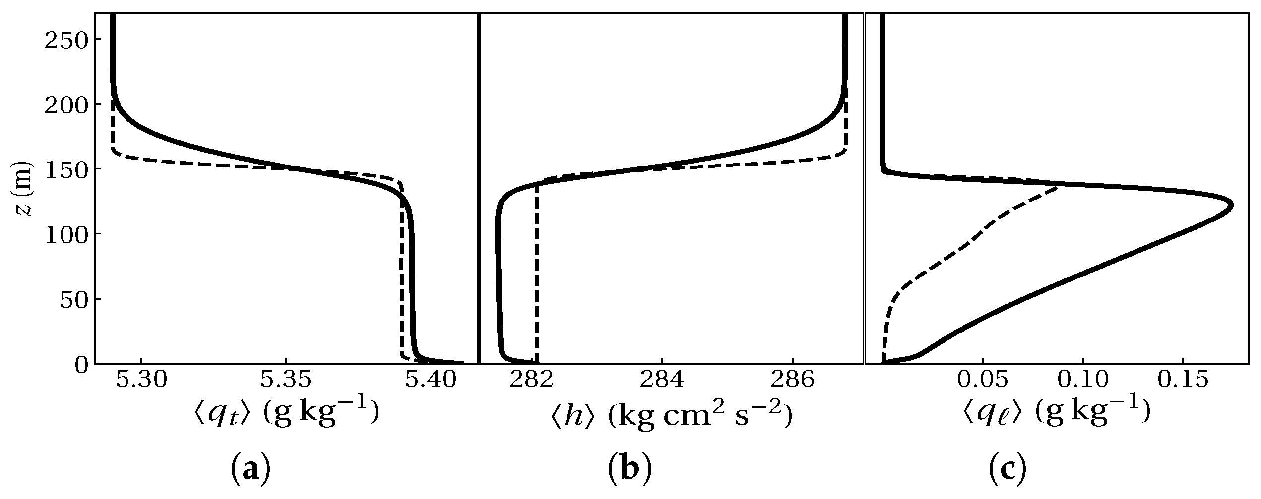
3.3. Sensitivity Studies

A series of sensitivity experiments were conducted. The details of simulation parameters are given in Table 1. We particularly paid attention to the forcings of inversion strength, relative humidity gradient, and greenhouse gas emission (manifesting in the form radiative cooling). For all cases, subsidence velocity was set to zero. In Table 1, the cases with changes in free tropospheric temperature are referred to with T; the cases with changes in specific humidity with Q; the cases with changes in the liquid-water lapse rate within the fog layer with L; and the cases with changes in the net radiative flux with R series. The scenarios of increasing the magnitude of humidity jump, intensifying the inversion strength, and reducing the moisture lapse rate are schematically depicted in Figure 1. Once fog is formed, we examine the sensitivity of fog dissipation to the warmer free troposphere by changing Δ θ , to the drier free troposphere (FT) by changing the relative humidity of free troposphere or Δ q t , and to the variation of the moisture lapse rate in the mixed layer by varying Γ q through changing the surface pressure, and to the radiative forcing (or the emission strength) in the FT by changing the net longwave radiative cooling at the fog-top F r , all identified in Equation (3) and quantitatively presented in Table 1.

4. Results

Fog evolution was examined by studying the LWP, TKE, boundary layer height and entrainment rate during the fog lifetime, once fog formed. We closely surveyed the temporal evolution of these variables until the fog layer approached the dissipation phase or close to fog depletion t ( LWP ) ent 0 . The inversion height or the fog boundary layer height, z i , is defined as the height of the minimum buoyancy flux. Finally, we discuss the possible mechanisms that can explain fog depletion under these aforementioned forcings. By visualization of the vertical structure of the fog layer, we argue how these sensitivity experiments can give us further insights to identify the dominant mechanism.

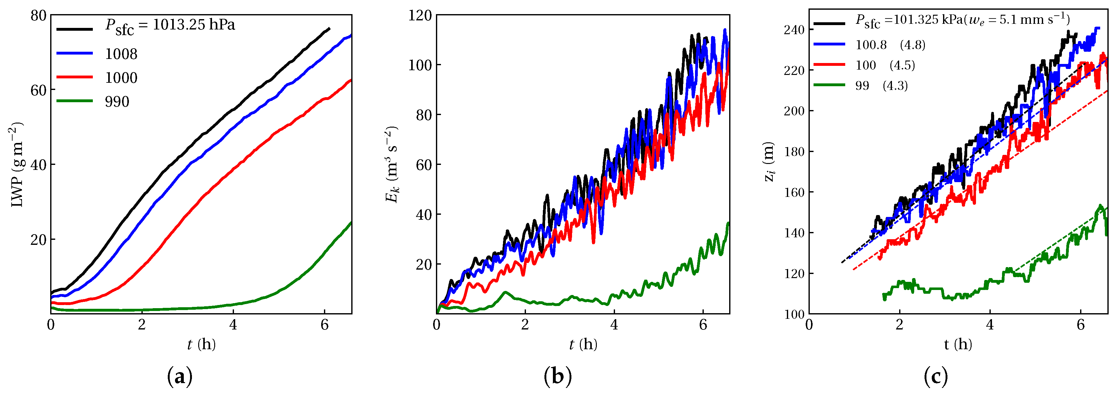
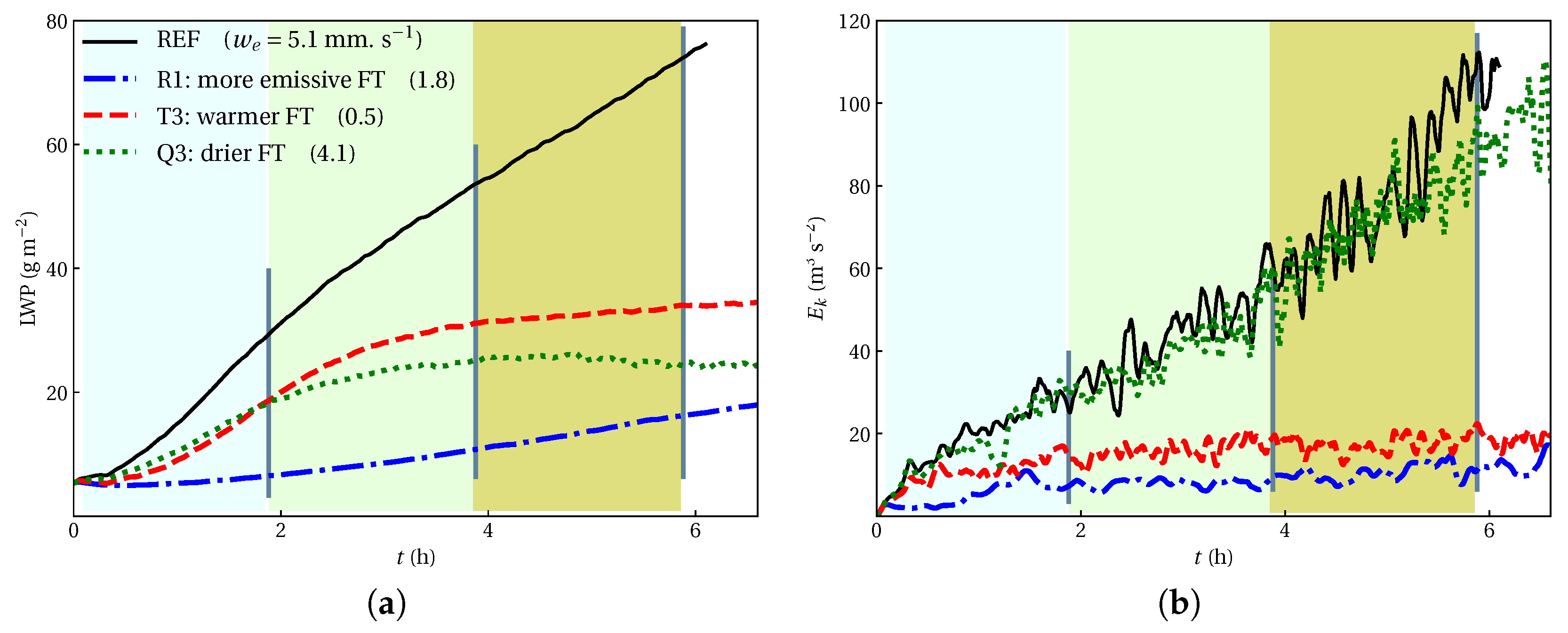
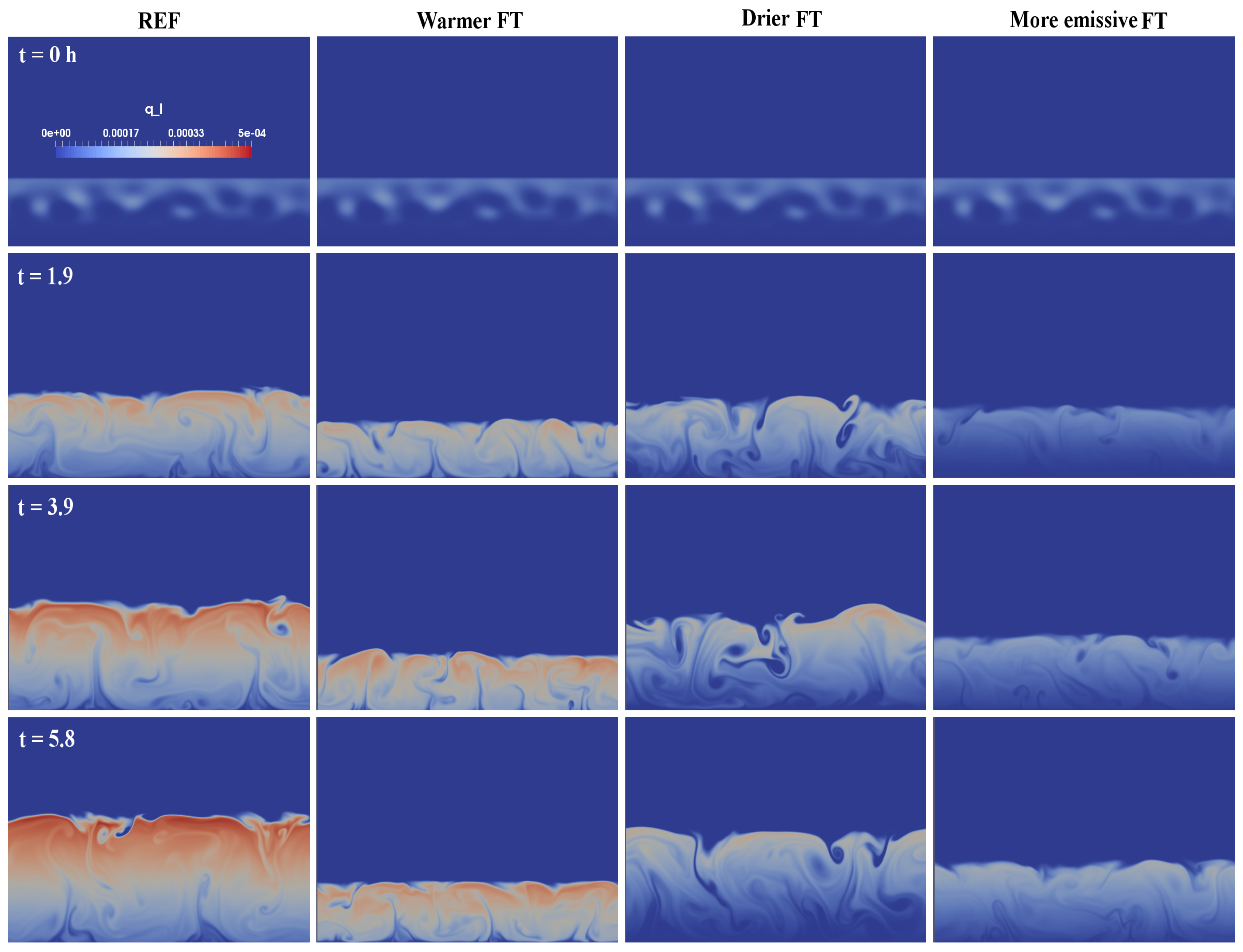
4.1. The Effect of the Free Troposphere Temperature

In LES studies of stratocumulus subject to the larger inversion strength, Bretherton et al. [33] and Bretherton and Blossey [60] show that warming free troposphere reduces entrainment rate, thickens the cloud layer, and lowers both the cloud-top and the cloud-base, leading to unchanged cloud geometrical thickness overall. Similarly, in the mixed-layer model studies of stratocumuli, de Roode et al. [61] and dal Gesso et al. [62] indicate that the stronger lower tropospheric stability diminishes the entrainment rate, but reduces the cloud layer depth with a consequent LWP reduction. Although the studies of the response of stratocumulus to the increase of inversion strength are not unanimous in thickening or thinning, they all confirm the suppression of entrainment rate in response to the larger inversion strength.
We expect a priori that larger inversion strength leads to reduction of fog LWP, as shown in Figure 2a. Keep in mind that the maximum inversion strength of the Paris Fog observation is Δ T = 7.8 K [40], whereas the typical value of Δ T = 5–10 K in the stratocumulus cases [36]. The response of fog to intensifying inversion strength seems to be similar to the one of a stratocumulus cloud to the same type of perturbation forcing. By warming FT, the level of turbulence within the fog layer is reduced, the inversion is lowered, and the boundary layer remains shallower compared to the REF case. Interestingly we noticed the equilibrium LWP tendency when the temperature jump rises fourfold with respect to the REF value. Using large-scale structure of q (discussed in Section 4.5), we observed that the fog layer with warmer FT contains more liquid water at a given height with respect to the REF case; thus, fog depletion does not occur though t LWP 0 . In Figure 2b, temporal evolution of the integrated TKE ( E k = ( 1 / 2 ) 0 z u i u i d ξ ) demonstrates that warmer FT inhibits the energetic inside fog as the fog layer tends to be shallower. That is due to the fact TKE is scaled by the convective velocity scale which depends on inversion height as E k w * 2 z i . Similar to stratocumuli, entrainment warming has negative feedback on the fog height, since the stronger inversion strength significantly reduces the entrainment of the FT air, as shown in Figure 2c.
The fog response to warmer FT is similar to the one of the stratocumulus boundary layer in a sense that the stronger inversion reduces turbulence mixing at the fog top. We also observe that despite the moderate reduction of LWP, warmer FT alone cannot lead to fog depletion, as t LWP 0 is not achieved. Warmer FT seems to aid with persistence of the fog rather than its depletion, under the assumption of the absence of shortwave radiation. That can be explained due to the absence of fog lifting mechanism, as explained in detail in Section 4.5.

4.2. The Effect of the Free Troposphere Relative Humidity

Studying the response of stratocumuli to drier FT reveals that entrainment rate remains unchanged, but entrainment drying increases, which eventually results in cloud thinning [33]. The mixed-layer model studies of stratocumulus clouds dal Gesso et al. [62] indicate that drier FT enhances the entrainment rate and LWP. However, they argue that depending on how parameterization of entrainment is formulated, LWP, and consequently entrainment can either increase or decrease. In sensitivity experiments of the drier FT (series Q in Table 1), free tropospheric total humidity q t is decreased uniformly, as schematically depicted in Figure 1, while retaining other parameters, such as the ones in the REF case. Drying FT can result in the direct effect of LWP reduction such that the LWP equilibrium can be reached if we dry FT at to least 20% of its REF case value. In other words, increasing total water content jump beyond | Δ q t | = 1.0 g · kg 1 tends to promote a reduction in LWP, as illustrated in Figure 3a. Evolution of TKE seems to be insensitive to the changes of the free tropospheric total humidity, as shown in Figure 3b. The growth of kinetic energy is maintained regardless of changing the moisture jumps. The reason is that since TKE is scaled by the convective velocity w * 2 = ( B 0 z i ) 2 / 3 , the slight drop of inversion height can be compensated a sufficient enhancement of radiative flux along the vertical dimension of the fog layer. Note that radiative cooling is the main source of TKE production at a cloud top (not shown here). The temporal evolution of the inversion height for a fog layer subject to different free tropospheric humidity presented in Figure 3c shows that while the entrainment rate is not reduced dramatically (from 5 mm · s 1 in the REF case to 4.3 mm · s 1 in the drier FT case), the tendency of LWP due to entrainment can approach zero, and fog begins to deplete.
As the magnitude of the total humidity jump at the inversion height ( Δ q t ) z i increases, e.g., via drying free troposphere, the entrainment rate slightly reduces as turbulent buoyancy production decreases. Drier FT promotes lifting the entire fog layer, while maintaining the energetics inside the fog layer. This finding is in agreement with the previous observation [24]. Fog response to the drier FT is similar to the stratocumulus response to the same perturbation, except that entrainment rate slightly drops, whereas the stratocumulus remains unchanged. Drier FT promotes fog lifting and fog dissipation as the LWP tendency starts becoming negative, while maintaining TKE within the fog layer.

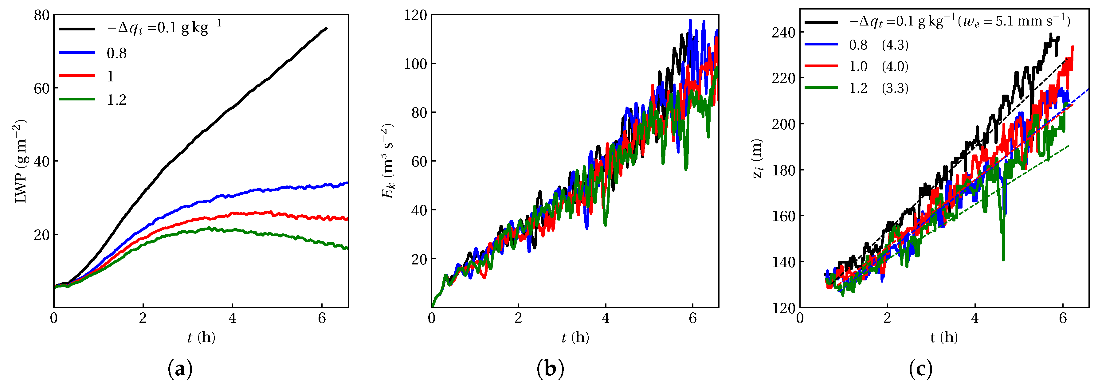
4.3. The Effect of Moisture Lapse Rate on Fog Depletion

To set up this experiment, we needed to reduce liquid-water lapse rate Γ q , as schematically shown in Figure 1c. To do so, one way is to change the specific humidity of water vapor, which itself is a function of surface pressure and temperature at the saturation point q s = f ( P s f c , T s f c ) . Another way is to change the shape of q profile such that its vertical gradient is reduced while there may be no guarantee to retain the initial total specific humidity the same as in the REF case. Therefore, we chose the first method and we decreased the liquid-water lapse rate by reducing surface pressure while keeping all parameters the same as the REF case. Keep in mind that the reduction of surface pressure in this case may not correspond to a real-world situation; we still used this exercise in a purely theoretical manner. Among all controlling factors highlighted in Equation (5), the role of Γ q on LWP tendency is rather more ambiguous than others. It is not simple to isolate the Γ q effect on LWP tendency as Γ q = f ( q t , θ ) . It seems that fog’s response to varying Γ q may exhibit the combined effects experienced in the two previous series of experiments, but not in a very straightforward manner due to the feedback between q t and θ . Due to different initial q l profiles, LWPs of different Γ q start at different values; nonetheless, they follow similar trends, as shown in Figure 4a. We observe that fog does not deplete under changing Γ q . Although in the case with the lowest surface pressure ( P s f c = 99 kPa), LWP tendency seems initially zero, it does not mean that fog depletes. As Γ q is very small and there is almost no fog formed initially. However, after about 4 h, as radiative cooling causes air temperature to reach its dew point, the fog layer starts thickening and TKE begins to grow at the same rate as for other cases, as shown in Figure 4b,c. The entrainment rate at the fog top is nearly insensitive to changes in the liquid-water lapse rate of the fog layer.

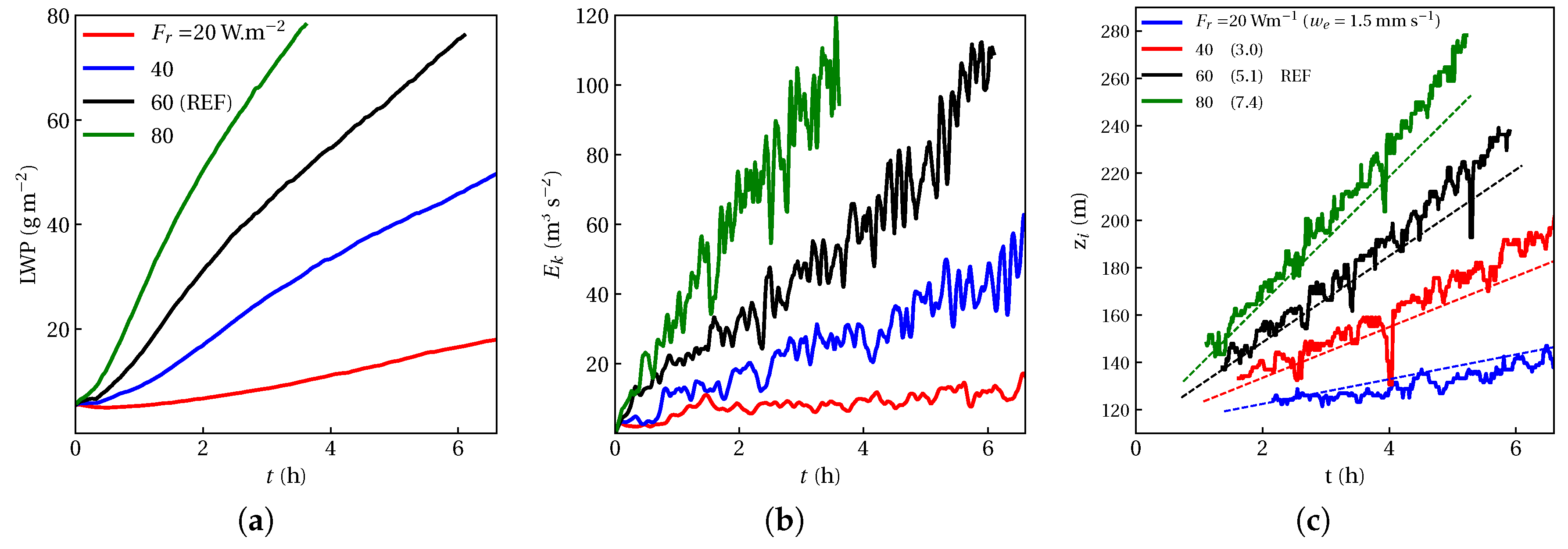
4.4. The Effect of Longwave Radiative Cooling

Radiative forcing has been identified as the predominant factor controlling cloud thinning in the well-mixed stratocumulus boundary layers [32,33]. In stratocumuli, reducing net radiative flux, F r , diminishes the entrainment rate as there is less turbulence production by cloud-top cooling. However, some uncertainties were observed in the previous findings. The LES study of Bretherton et al. [33] suggested that reducing F r leads to a cloud thinning which is in contrast to the mixed-layer model study of dal Gesso et al. [62]—that reducing F r makes the stratocumulus-topped boundary layer moister and warmer with respect to their reference case. Although the critical role of radiative cooling on fog evolution has been previously recognized [63,64,65], how this forcing per se can modify fog depletion phase has not been systematically examined yet. To that end, in this experiment (series R in Table 1), we changed the net longwave radiative flux, while keeping other parameters the same as in the REF case. To impose such a forcing perturbation on the fog layer, we made FT more emissive by increasing downwelling longwave radiation, and thus reducing the net longwave at fog top.
We observed that fog evolution was highly sensitive to changes in the radiative forcing which affects LWP tendency via two pathways. One pathway is through changing the cooling rate in the mixed layer directly. Another pathway is associated with the indirect effect on the fog-top entrainment rate. Figure 5a depicts that despite the reduction of LWP by reducing F r , this forcing alone cannot deplete the fog even if the net F r is reduced by threefold with respect to the REF case. Decreasing net longwave radiative flux stabilizes the fog layer, as shown in Figure 5b. As more radiatively cooled air is transported downward by turbulent eddies, more cooling in the sub-cloud layer occurs; thus, substantially lowering the fog-top (Figure 5c). Consequently, less turbulence production by the fog-top radiative cooling inhibits entrainment at the fog top. We infer that reducing longwave radiative flux as a forcing perturbation cannot promote fog depletion single-handedly, though it diminishes LWP. Therefore, more emissive FT results in reducing the turbulent flux of total water content, w q t z i ; thus, less mixing at the fog top hinders fog lifting—one of key mechanisms suggested for fog dissipation, which is discussed in the next section.

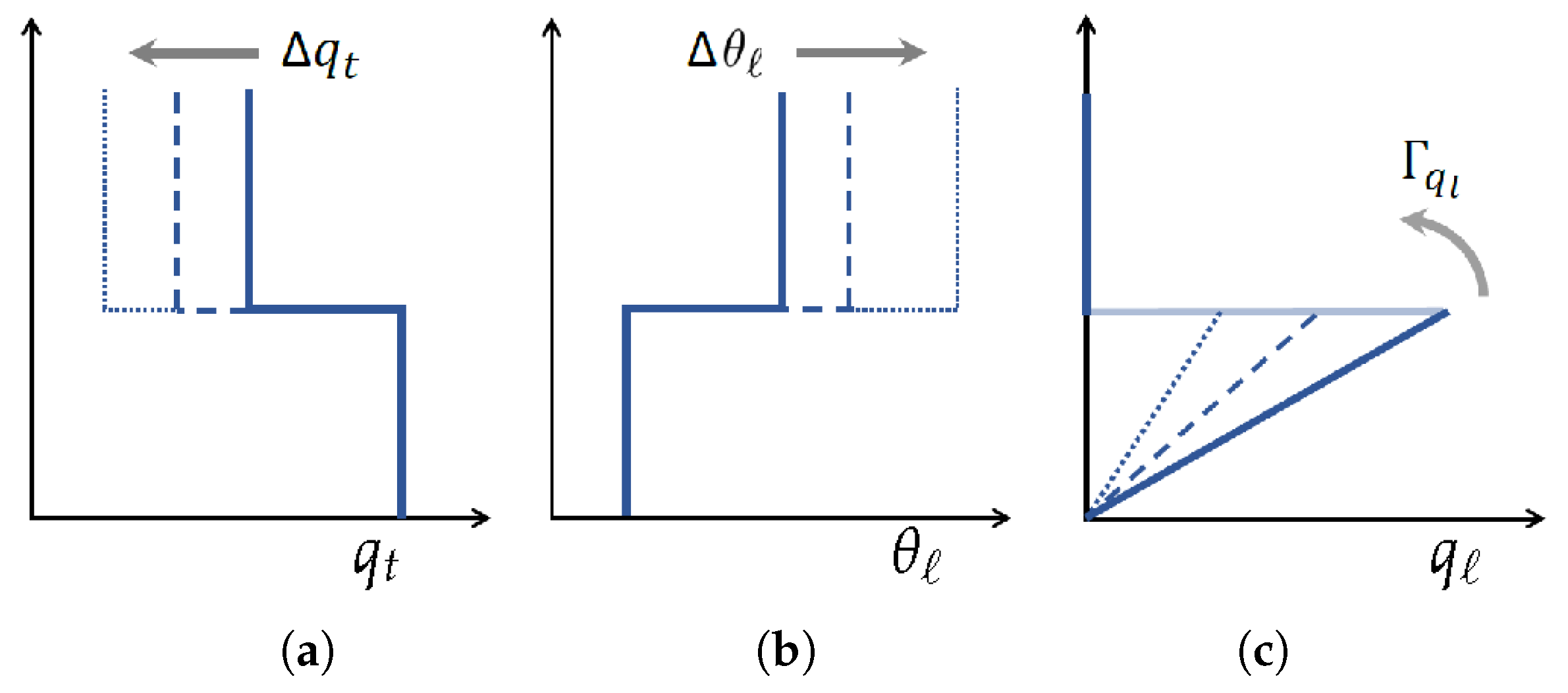
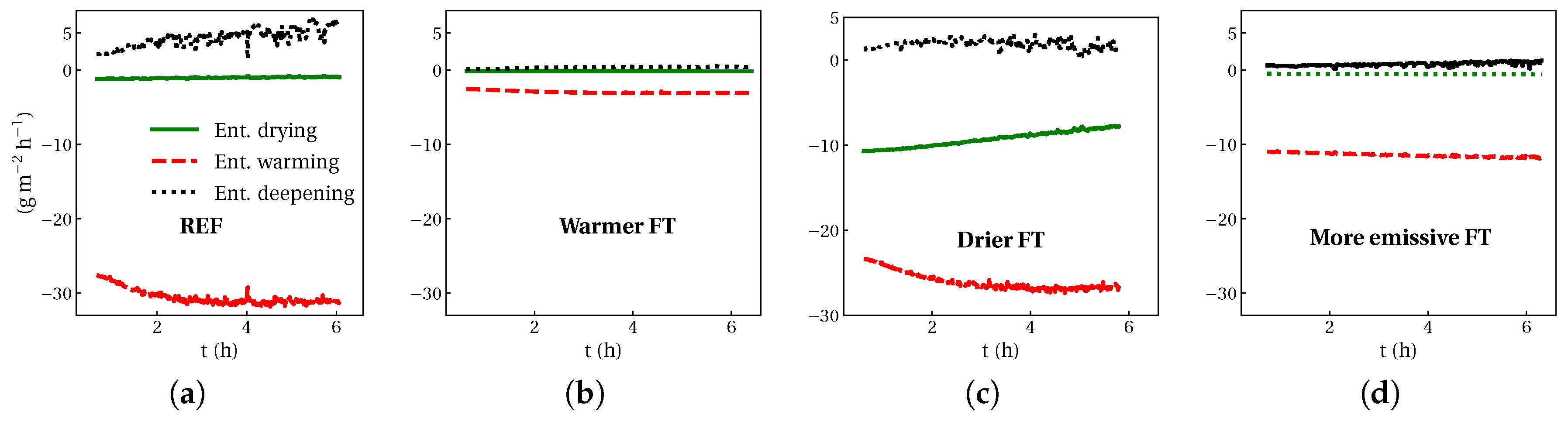
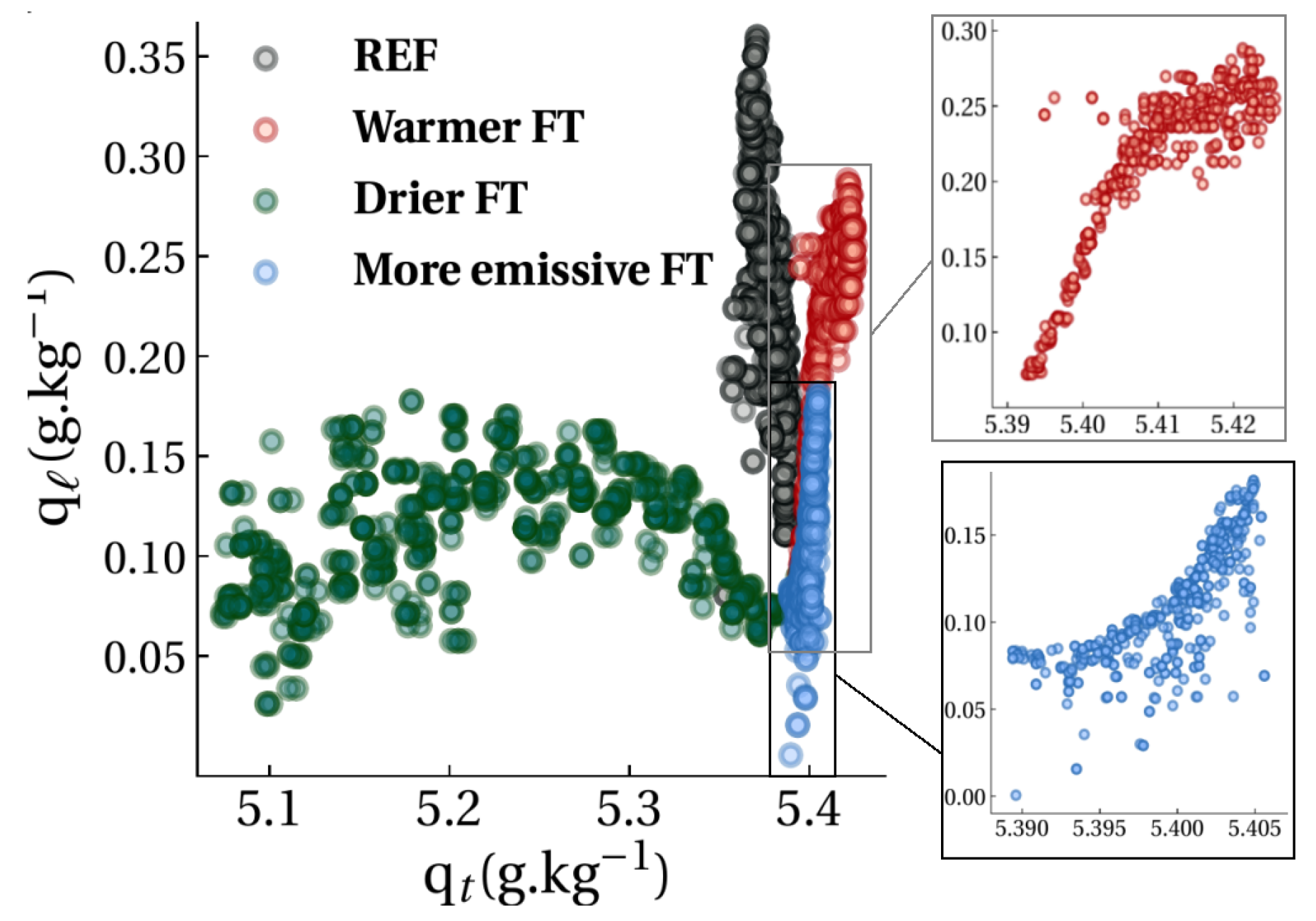
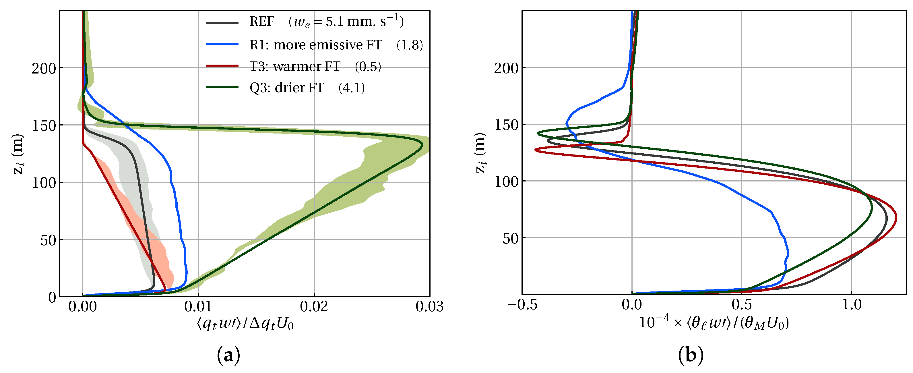
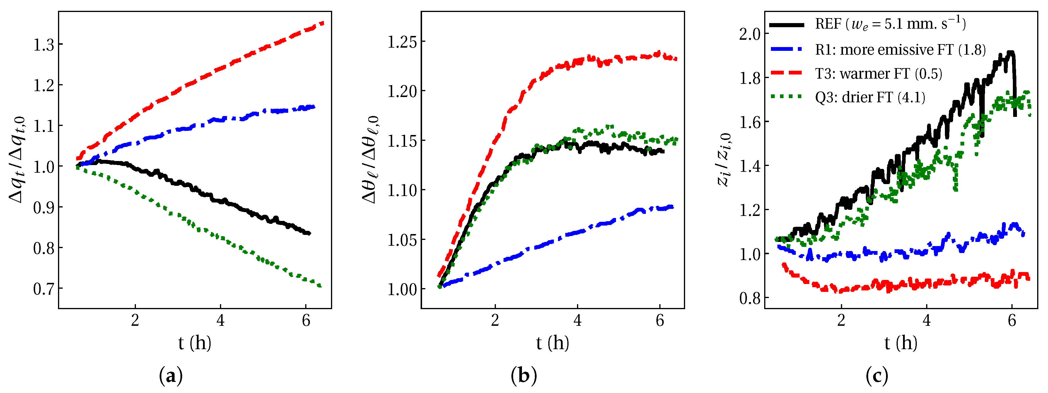
4.5. Fog Depletion Mechanisms

Phenomenologically speaking, fog depletion can be explained by two possible mechanisms. The first mechanism is fog lifting by radiation penetrating the fog layer. Subsequent warming of the surface layer promotes formation of updrafts, leading to fog depletion initiated by warming the surface, following by propagating upwards through updrafts impinging upon the fog top. The second proposed mechanism for fog depletion is inward mixing, in which fog erosion occurs inwards from its edges at the fog top. It is argued that fog becomes thinner by inward mixing, but it does not disappear altogether in a spatially uniform manner [18]. The observation of the geostationary satellite imagery has been interpreted as fog dissipating from its outer edge inward rather than it burning off as a whole [66]. Inward mixing is the result of a weak circulation on the outer edge of fog. Such mixing entrains warmer and drier air of the free troposphere into the fog layer and eventually erodes the fog from the edges by mixing rather than by lifting the fog layer. The process of inward mixing continues until fog completely dissipates without necessarily being lifted. The key difference between these two mechanisms is where the onset of fog depletion occurs. Fog depletion via the lifting mechanism initiates from the surface layer and finds its way up through updraft and raising the inversion layer. Inward mixing initiates fog depletion by facilitating entrainment of dry air into the fog layer, commonly at the fog top, regardless of affecting the inversion height. Besides these two mechanisms, shortwave heating of the fog layer can also play a crucial role in depletion toward the end of the fog cycle.
To investigate which mechanism plays a dominant role on fog depletion in the current sensitivity experiments, we selected three cases of reduced radiative cooling or more emissive FT (case R1), warmer FT (case T3), and drier FT (case Q2), and compared them against the REF case. For details of cases, see Table 1. The selection criterion is based on the capacity of fog to reach equilibrium: t ( LWP ) 0 . For the sake of a more convenient comparison, we revisit the temporal evolution of LWP and TKE of these cases in a new plot shown in Figure 6. To better connect the temporal evolution of the fog layer with its vertical structure, we compare the structures of fog at the times marked in Figure 6, relevant to the start of maturity phase, and close to the onset of fog depletion. The large-scale structure of the fog response to three different idealized forcing perturbation is compared by examining the vertical structure of liquid water specific humidity in Figure 7. In each row, we present a time snapshot that can give us a perspective toward a more meaningful narrative of the physical interpretation of fog evolution. The first row shows the initial stage which is identical for all experiments.
In REF case as shown in Figure 7 (REF column), the fog layer deepens ( w e = 5 mm · s 1 ) and the LWC of the fog layer increases over time. The fog layer is characterized by much less LWC in the more emissive FT case, pre-conditioning a faster dissipation once the sun rises. In both cases of warmer FT and more emissive FT, the fog top is lowered with respect to the REF case but fog hardly dissipates. In the warmer FT case, the reason is that the stronger temperature inversion hinders entrainment ( w e = 0.5 mm · s 1 ), leading to the augmentation of LWC within the fog layer and fog-thickening, as shown in Figure 7 (warmer FT column). In the more emissive FT case, despite tracing the signature of dry tongues (as early as ∼2 h), the entrainment rate ( w e = 1.8 mm · s 1 ) is not high enough to lift the fog top; thus, fog persists, as shown in Figure 7 (more emissive FT column). There is a pronounced difference between the vertical structure of the drier FT illustrated in Figure 7 (drier FT column) and other cases, as the presence of dry tongues at the fog-top region is distinctly noticeable, even as early time as t = 2 h. Drier air from the non-turbulent FT can sink down into the fog layer through these holes. Erosion of the fog layer at the top via inward mixing can cause the cellular pattern or patchiness of the fog that eventually contributes to fog depletion, particularly in the fog-top entrainment zone. Despite the relatively small fractional area of the dry tongues or cloud-holes at the fog-top, these volumes of dry air play a significant role on the LWC variability and can contribute to reduction of LWP, as shown in Figure 6a, in the case of drier FT. Thus, zero LWP tendency is achieved earlier than any other cases. Additionally, it is interesting to observe that simultaneously fog lifting in the case of drier FT fosters fog depletion near the surface, as shown in the last snapshot of Figure 7 (drier FT column). Since w e in the drier FT experiment is nearly sustained with respect to the REF case, as shown in Figure 3c, the entrainment into the descending thermals can gradually erode fog downward as a result of inward mixing, while fog lifting fosters drying the surface layer simultaneously.

5. Discussion

To focus on the entrainment contribution to the LWP tendency of the cases selected in Figure 6, we examined the temporal evolution of each term presented in Equation (5); namely, entrainment drying, entrainment warming, and fog layer deepening due to entrainment. But before that, we present our examination of the temporal evolution highlighted terms in Equation (7) contributing to these effects: Δ q t , Δ θ , and inversion height z i presented in Figure 8.
Since simulation of each sensitivity case is initialized with different value of Δ q t or Δ θ , we normalized each variable with its initial value to conduct a meaningful comparison among cases. Using the profile of θ variance, the upper and lower boundaries of the inversion layer were determined by following the work of Yamaguchi et al. [67]. The magnitude of the inversion jump of humidity decreases the most for the drier FT compared to other cases, as shown in Figure 8a, which causes more entrainment drying, as the entrainment velocity is almost sustained with respect to the REF case. Entrainment warming is barely affected by drying FT with the respect to REF case, as shown in Figure 8b. In all cases except the reduced radiation (or more emissive FT), the inversion strength reaches a saturation point within less than 3 h after start of the simulation and stops growing. The growth rate of the inversion strength in both cases of REF and drier FT are comparable as their growth rate of the inversion height (the mean entrainment rate) shown in Figure 8c is similar.
Budget of the LWP tendency due to different entrainment contributions detailed in Equation (7) is shown in Figure 9. The entrainment drying term exhibits the most profoundly different contribution to fog evolution among these cases. Only in the drier FT case, entrainment drying increases (Figure 9c); thus, it contributes to fog depletion. The fog layer deepening due to entrainment ( L in Equation (7)) is only significant in REF case, and is to some extent noticeable in the drier FT case, since this term is dependent on the maximum value of the LWC inside the fog layer, which is proportional to the fog layer depth (∼ z i ). Regarding the role of entrainment on the LWP tendency, both warmer FT and more emissive FT cases exhibit similarities (Figure 9b,d). The contribution of entrainment drying and entrainment deepening is negligible, as in both cases fog persists and it does not lift off the ground. The more emissive FT case has more entrainment warming as its net radiative flux is three times less than the warmer FT case; thus, more radiative cooling is observed. We conclude that entrainment drying is more effective than entrainment warming for fog depletion.
The distribution of dry fog parcels during maturity and dissipation phases, as defined by Nakanishi [9], is depicted in Figure 10. Although all sensitivity experiments were initialized with the same liquid water content, drier FT cases compared with other cases exhibited a very different trend of moisture evolution in the fog layer. As shown in Figure 10, only in the drier FT case, was the higher total mixing ratio associated with more of the drier fog parcels (lower q ), whereas in the warmer FT and more emissive FT, the wetter fog parcels with more liquid water have a higher total mixing ratio. This confirms the fact that the reduction in drop concentration is not only due to drop dilution with saturated air, but also due to drop removal by evaporation within the fog layer.
The question of fog depletion or fog persistence can be framed in terms of moisture mixing. To identify where the mixing of moisture is enhanced locally, vertical profiles of moisture fluxes were examined. The vertical structures of liquid-water specific humidity q w in all cases are nearly identical (not shown here). However, the vertical profiles of turbulent flux of the the total water content q t w in the all cases are distinctly different from the the drier FT case, as shown in Figure 11a. Drying FT facilitates moisture removal in the region close to the fog-top more effectively than other cases, in contrast with other two forcing perturbations that moisten the fog layer, while turbulent heat flux exhibits comparable behavior except in the case of a more emissive FT, where less warming takes place within the fog layer, as shown in Figure 11b.

6. Conclusions and Perspectives

Fog maintenance and dissipation are highly dependent on the regulation of competing physical processes. The relevant feedback acting to regulate turbulent kinetic energy (TKE), liquid water path (LWP), and the entrainment rate of the fog layer can be illustrated in a conceptual diagram similar to the one for the stratocumulus clouds [36]. Although such a conceptual description is suggested for the marine stratocumulus, we may need to take caution extending that framework to fog due to differences in inversion height, life-time, the role of exchanges with the surface, shorter time-scales of regulating feedbacks in fog, and its highly transient nature. To that end, we performed a series of sensitivity studies of radiation fog based on the Paris Fog observational data [40]. DNS of a fog layer was performed at such high resolution that turbulence processes were able to be resolved down to centimeter scales. We changed the forcing perturbations to imitate the realistic environmental changes in temperature, relative humidity, and radiation. The roles of turbulent transport of heat, moisture, and radiative cooling on the fog evolution, especially on the depletion phase, were investigated by analyzing the temporal evolution of LWP, the TKE, and the inversion height of the fog boundary layer.
First, increasing inversion strengths by the warming free troposphere (FT) was found to decrease entrainment rate due to the inhibition of fog-top mixing. The resulting fog layer is shallower compared to the reference case. Under such a thermodynamic forcing, fog may deepen (as LWP increases), or become shallower (as inversion drops), but it may not deplete. Second, under another thermodynamic forcing, in the drier FT, as opposed to other cases, LWP decreases while fog top keeps rising; thus, the turbulence intensity of the fog layer keeps growing. Unlike the stratocumulus, in which a larger moisture jump at the inversion allows a smaller cloud thickness to sustain the same entrainment, the fog-top entrainment rate slightly drops but TKE keeps increasing. Fog thins and eventually depletes due to the fog lifting mechanism accompanying inward mixing as the fog becomes more horizontally heterogeneous in structure. Third, reduced net longwave radiation lowers the fog top. Less fog-top radiative cooling generates less turbulence with respect to the reference case; thus, less fog-top entrainment. Although the fog inversion drops and LWC variability decreases, fog does not deplete. Fog response seems to be different from the response of stratocumulus clouds to the same perturbation. We postulate that such a difference may be due to the interference of surface dynamics in the fog layer, as the boundary layer depth of fog is ten times less than stratocumulus clouds’ top boundary layers. Thus, decoupling with the subcloud layer due to liquid-water flux observed in stratocumulus may not occur in the fog layer. By examining the contribution of velocity variances to TKE, we infer that a key to fog depletion is maintaining the growth of energetics inside the fog layer while reaching the LWP equilibrium.
The primary control factor in fog dissipation was identified as the environmental perturbation that can maintain the energetics of fog by sustaining the entrainment rate at the fog top while reducing LWP. Among all thermodynamic forcings, fog depletion is more sensitive to the moisture gradient at the inversion height rather than the inversion strength or lapse rate of liquid water content in the mixed layer. We suggest that the increased humidity jump is the key factor controlling fog depletion among all possible thermodynamic forcings.
The findings of the present study can be applied to the studies that consider the temporal evolution of fog subject to changes in the weather and climate conditions. Besides the environmental perturbations examined here, there are indeed more parameters controlling fog dissipation phase, such as moisture sedimentation and surface fluxes. Further study in identifying the role of subsidence velocity on fog dissipation is under way as an extension of the current work. Finally, direct numerical simulation (DNS) can be promoted as a useful tool to assess the hypotheses and accuracies of the numerical frameworks for studying fog processes, as it is particularly useful when turbulent processes are critically important. Although the present study is the first attempt to use DNS to discuss the sensitivity of fog dissipation to changing environmental conditions, more progress can be achieved by using such a promising tool in the atmospheric and climate research community.

Funding

The author gratefully acknowledges the Gauss Centre for Supercomputing for providing computing time at Jülich Supercomputing Centre. Funding was provided by the Max Planck Society through Turbulent Mixing Processes in the Earth System. Primary data and scripts used in the analysis and other supporting information that may be useful in reproducing the author’s work are archived by the Max Planck Institute for Meteorology.

Acknowledgments

The author would like to express sincere gratitude to Juan Pedro Mellado who helped and consulted in the development of this work during the author’s stay in the Max Planck Institute for Meteorology, and also for the computation resources offered by the German Climate Computing Centre. The useful discussions and constructive suggestions of the three anonymous reviewers who helped to improve the original manuscript are greatly appreciated.

Conflicts of Interest

The authors declare no conflict of interest.

Abbreviations

The following abbreviations are used in this manuscript:
DNSdirect numerical simulation
FTfree troposphere
LESlarge eddy simulation
LWCliquid water content
LWPliquid water path
TKEturbulent kinetic energy

Appendix A. Problem Formulation

We performed a three-dimensional direct numerical simulation of a shallow atmospheric boundary layer with a multi-phase flow fluid which is disperse (small Stokes numbers < 10 2 and moderate settling numbers 0.5 ) and dilute (liquid volume fraction 10 6 ). Under the anelastic approximation, we solved the Navier–Stokes equations plus the transport equations for enthalpy, h, total water specific humidity, q t , and liquid-water specific humidity, q , in an Eulerian framework, as follows:
. ( ρ 0 u ) = 0 ,
ρ 0 D u = p + Re 1 2 u + ρ 0 b k + ρ 0 w z u ,
ρ 0 D h = . [ ρ κ h h ρ j ( h h ) ρ j r ] + ρ 0 w z h ,
ρ 0 D q t = . [ ρ κ v q t ρ j ( 1 q t ) ] + ρ 0 w z q t ,
ρ 0 D q = . [ ρ κ v q ρ j ( 1 q ) ] + ρ 0 w z q + ρ ( t q ) p h a ,
where D is the material derivative operator; ρ 0 is the reference density; u is the velocity vector field; p is hydrostatic pressure; and b g ( ρ ρ 0 ) / ρ 0 is buoyancy defined, where g is the magnitude of the gravitational acceleration, k is the unit vector in the upward z-direction, w is the large-scale subsidence velocity, and h [ c d + q t ( c v c d ) ] T q L v + g z is the static energy of liquid-water, where h = h ( q = 1 ) . The specific heat capacities at constant pressure of dry air and of waver vapor are c d and c v , respectively. The enthalpy of vaporization of water was used as L v = 2.4429 ( MJ kg 1 ). The total water specific humidity and the liquid-water specific humidity are denoted by q t and q , respectively.
The longwave radiative flux ( ρ j r ) was modeled as follows [58]:
ρ j r = ρ 0 q α | | ρ j r | | c t e LWP z / α | | ρ j r | | c b e ( LWP 0 LWP z ) / α k ,
where the LWP at the height z defined as
LWP z z z ρ 0 q d z .
The nondimensional radiative parameter is α = ρ 0 κ L 0 1 , where L 0 is the initial inversion height and κ is the absorptivity factor or extinction coefficient which depends on fog microphysics structure. Here we assume the value of κ = 120 (m 2 /kg) as used by [37]. To include fog microphysics in our simulation, one can consider two important phenomena of gravitational settling and phase relaxation which are encapsulated in the liquid-water mass flux ρ j and the time-rate of phase-change (e.g., condensation) ρ ( t q ) p h a . The liquid-water mass flux accounts for the fluxes due to gravitational settling of fog droplets and differential diffusion effects. Here, the liquid-water mass fluxes used in our simulation were modeled by [68]:
ρ j = α m ρ q w s k + ρ κ v κ 1 q q ,
where α m is the coefficient representing the effect of having droplets with different sizes, as the typical range of fog droplet radius is 1–15 ( μ m ) [1]. The reference settling velocity of droplet is denoted by w s which is the function of droplet diameter, its density, and the dynamic viscosity of the gas that the droplet settles in. Typical values of droplet settling velocity can be comparable to the typical value of the mean entrainment velocity at a cloud-top. Therefore, gravitational settling can counteract the forcing caused by radiative or evaporative cooling through depleting the liquid-water at the fog-top region and ultimately through altering fog-top dynamics. Based on this concept, one of the very first ideas of artificial fog dissipation used fog seeding by salt particles [69]. Another effect is due to differential diffusion of droplets, which is the second term in Equation (A4), where κ is diffusion coefficient of liquid phase into the gaseous phase. For typical atmospheric conditions, the diffusion of waver vapor phase dominates the diffusion of the liquid phase ( κ κ v ) [70]. However, it was shown that reducing κ results in reduction of entrainment velocity when radiative cooling is the major turbulence generator at the cloud-top region [71]. Another microphysical effect that includes in the current simulation is the phase relaxation or the rate of phase-change (e.g., condensation) which is modeled by:
ρ ( t q ) p h a = α p ρ q q v / q s 1 t p ,
where α p is similar to α m in Equation (A4) which accounts for different sizes of droplets but the droplets that are involved with the phase change. Equation (A5) is ratio of the supersaturation to the phase relation time of a droplet t p . For evaluating both α p ad α m , the knowledge of droplet size distribution is required. The DNS code solves the evolution equations of Equation (A1) based on the the discretization scheme of the pseudo-spectral compact Padé [72], while the time-advancement is performed using the low-storage Runge–Kutta scheme [73]. Having validated for cloud-topped boundary layers [71,74], the source files of the computational of DNS code are open-source and can be found at https://github.com/turbulencia/tlab.

Appendix B. Convergence Study and Initialization

Using a Cartesian coordinates, the governing equations of Equation (A1) are solved in a structured grid, which is constructed by building up three directions separately. Each direction direction is broken into different segments, following a specific generation algorithm. First, we construct a basic grid with uniform spacing of s j : = c 0 ( j ) ; j = 1 , . . , N , where c 0 is the uniform value and N is the grid size. On the lateral plane, for both x and y directions, we use a uniform spacing c 0 = 6.67 . However for the vertical direction, the non-uniform spacing is constructed by the two-transition mapping function using a hyperbolic tangent given by
d x d s = 1 + c 1 / c 0 1 2 1 + tanh s s t 1 2 δ 1 ) ,
where the grid step Δ x = d x / d s j varies between the uniform value of c 0 and c 1 and transition occurring at s = s t 1 over the length of δ 1 . A similar notation applied to the second transition mapping in the second part of RHS of Equation (A6). Note that other explicit mapping, such as Equation (A6) can be used to initialize the vertical profile of the q t and h, shown in Figure A1, in order to capture the gradient at the surface and also at the inversion height.
The dependence of the results on Reynolds number, and thus the size range of the resolved scales, was investigated by studying the temporal evolution of the vertically integrated turbulent kinetic energy and liquid water path. Figure A2 demonstrates that the difference between the two largest Reynolds numbers starts to be small enough to extrapolate part of the results to atmospheric conditions (Reynolds-number similarity theory [57]). Note that the grid resolution convergence was studied according to the Reynolds number based on the grid spacing, as the numerical uncertainty of DNS is associated with this parameter. Here the Reynolds number corresponds to the grid spacing; the larger the R e , the finer the grid. The grid convergence studies were performed for two sets of observational data of different structures of radiation fog layer: a fog event with a lower-in-moister troposphere compared to the fog layer—Cabauw fog in August 1977 [37], and a fog event with a drier free troposphere than the fog layer—Paris Fog on the night of 18/19 February 2007 [40]. To have a better picture on initialization procedure of current simulation, the initial profiles of the REF case simulation at 00:30 UTC and and 3 h later are shown in Figure A1. The evolution of vertical profile of prognostic variable and q are presented as fog evolves from maturity phase toward dissipation phase. Figure A1c demonstrates that the surface layer is initially dry but the fog layer thickens as LWC starts to increases.
Figure A1. Vertical profile of (a) the total water content, (b) mean enthalpy, and (c) liquid water content of REF simulated based on the Paris Fog data. Dashed lines are initial vertical profiles at 00:30 UTC and solid lines are profiles at 3 h later.
Atmosphere 11 00012 g0a1
Figure A2. Temporal evolution of (a) vertically integrated TKE and (b) LWP (for the Paris fog for various Reynolds numbers).
Atmosphere 11 00012 g0a2

References

  1. Lohmann, U.; Lüönd, F.; Mahrt, F. An Introduction to Clouds: From the Microscale to Climate; Cambridge University Press: Cambridge, UK, 2000. [Google Scholar]
  2. Tardif, R.; Rasmussen, R.M. Event-Based Climatology and Typology of Fog in the New York City Region. J. Appl. Meteorol. Climatol. 2007, 46, 1141–1168. [Google Scholar] [CrossRef] [Green Version]
  3. Syed, B.F.S.; Kornich, H.; Tjernstrom, M. On the fog variability over south Asia. Clim. Dyn. 2012, 39, 1993–2005. [Google Scholar] [CrossRef]
  4. Li, Z.; Eck, T.; Zhang, Y.X.; Zhang, D.L.; Li, L.; Xu, H.; Hou, W.; Lv, Y.; Goloub, P.; Gua, X. Observations of residual submicron fine aerosol particles related to cloud and fog processing during a major pollution event in Beijing. Atmos. Environ. 2014, 86, 187–192. [Google Scholar] [CrossRef]
  5. Agarwal, A.; Mangal, A.; Satsangi, A.; Lakhani, A.; Kumari, K. Characterization, sources and health risk analysis of PM 2.5 bound metals during foggy and non-foggy days in sub-urban atmosphere of Agra. Atmos. Res. 2017, 197, 121–131. [Google Scholar] [CrossRef]
  6. Gultepe, I.; Tardif, R.; Michaelides, C.; Cermak, J.; Bott, A.; Bendix, J.; Mueller, M.D.; Pagowski, M.; Hansen, B.; Ellrod, G.; et al. Fog Research: A Review of Past Achievements and Future Perspectives. Pure Appl. Geophys. 2007, 164, 1121–1159. [Google Scholar] [CrossRef]
  7. Johnstone, J.A.; Dawson, T.E. Climatic context and ecological implications of summer fog decline in the coast redwood region. Proc. Natl. Acad. Sci. USA 2010, 107, 4533–4538. [Google Scholar] [CrossRef] [PubMed] [Green Version]
  8. Baldocchi, D.; Waller, E. Winter fog is decreasing in the fruit growing region of the Central Valley of California. Geophys. Res. Lett. 2014, 41, 3251–3256. [Google Scholar] [CrossRef]
  9. Nakanishi, M. Large-eddy simulation of radiation fog. Bound.-Layer Meteorol. 2000, 94, 461–493. [Google Scholar] [CrossRef]
  10. Maronga, B.; Bosveld, F.C. Key parameters for the life cycle of nocturnal radiation fog. Q. J. R. Meteorol. Soc. 2017, 143, 2463–2480. [Google Scholar] [CrossRef]
  11. Bergot, T.; Escobar, J.; Masson, V. Effect of small-scale surface heterogeneities and buildings on radiation fog Large-eddy simulation study at Paris–Charles de Gaulle airport. Q. J. R. Meteorol. Soc. 2015, 141, 285–298. [Google Scholar] [CrossRef]
  12. Teixeira, J. Simulation of fog with the ECMWF prognostic cloud scheme. Q. J. R. Meteorol. Soc. 1999, 125, 529–552. [Google Scholar] [CrossRef]
  13. Zhou, B.; Du, J. Fog prediction from a multimodel mesoscale ensemble prediction system. Weather Forecast. 2010, 25, 303–322. [Google Scholar] [CrossRef]
  14. Roman-Cascon, C.; Steeneveld, G.J.; Arrillaga, C.Y.J.A.; Maqueda, G. Forecasting radiation fog at climatologically contrasting sites: Evaluation of statistical methods and WRF. Q. J. R. Meteorol. Soc. 2016, 142, 048–1063. [Google Scholar] [CrossRef]
  15. Guedalia, D.; Bergot, T. Numerical forecasting of radiation fog. Part II: A comparison of model simulations with several observed fog events. Mon. Weather Rev. 1994, 122, 1231–1246. [Google Scholar] [CrossRef] [Green Version]
  16. Teixeira, J.; Miranda, P. Fog prediction at Lisbon airport using a one-dimensional boundary layer model. Meteorol. Appl. 2001, 8, 497–505. [Google Scholar] [CrossRef]
  17. Price, J.D. On the Formation and Development of Radiation Fog: An Observational Study. Bound.-Layer Meteorol. 2019, 172, 167–197. [Google Scholar] [CrossRef]
  18. Roach, W.T.; Brown, R.; Caughey, S.J.; Garland, J.; Readings, C. The Physics of radiation fog. I: A field study. Q. J. R. Meteorol. Soc. 1976, 102, 313–333. [Google Scholar] [CrossRef]
  19. Duynkerke, P.G. Turbulence radiation and fog in Dutch stable boundary layers. Bound.-Layer Meteorol. 1999, 90, 447–477. [Google Scholar] [CrossRef]
  20. Welch, R.M.; Wielicki, R.A. The stratocumulus nature of fog. J. Appl. Meteorol.Climatol. 1986, 25, 101–111. [Google Scholar] [CrossRef] [Green Version]
  21. Steeneveld, G.J.; Ronda, R.J.; Holtslag, A.A.M. The challenge of forecasting the onset and development of radiation fog using mesoscale atmospheric model. Bound.-Layer Meteorol. 2015, 1354, 265–289. [Google Scholar] [CrossRef]
  22. Nicholls, S. The Dynamics of Stratocumulus: Aircraft Observations and Comparison with a Mixed Layer Model. Q. J. R. Meteorol. Soc. 1984, 110, 783–820. [Google Scholar] [CrossRef]
  23. Huang, H.; Liu, H.N.; Jiang, W.M.; Huang, J.; Mao, W.K. Characteristics of the Boundary Layer Structure of Sea Fog on the Coast of Southern China. Adv. Atmos. Sci. 2011, 28, 1377–1389. [Google Scholar] [CrossRef]
  24. Ye, X.; Wu, B.; Zhang, H. The turbulent structure and transport in fog layers observed over the Tianjin area. Atmos. Res. 2015, 153, 217–234. [Google Scholar] [CrossRef]
  25. Barker, E.H. A maritime boundary-layer model for the prediction of fog. Bound.-Layer Meteorol. 1977, 11, 267–294. [Google Scholar] [CrossRef]
  26. Koračin, D.; Rogers, D.P. Numerical Simulations of the Response of the Marine Atmosphere to Ocean Forcing. J. Atmos. Sci. 1990, 47, 3336–3349. [Google Scholar] [CrossRef] [Green Version]
  27. Koračin, D.; Businger, J.A.; Dorman, C.E.; Lewis, J.M. Formation Evolution and Dissipation of Coastal Sea Fog. Bound.-Layer Meteorol. 2005, 117, 447–478. [Google Scholar] [CrossRef]
  28. Bergot, T.; Terradellas, E.; Cuxart, J.A.; Mira, O.; Liechti, M.M.; Nielsen, N.W. Intercomparison of single-column numerical models for the prediction of radiation fog. Mon. Weather Rev. 2007, 46, 504–521. [Google Scholar]
  29. Telford, J.W.; Chai, S.K. Marine fog and its dissipation over warm water. J. Atmos. Sci. 1993, 50, 3336–3349. [Google Scholar] [CrossRef] [Green Version]
  30. Lundquist, J.D.; Bourcy, T.B. California and Oregon Humidity and Coastal Fog. In Proceedings of the 14th Conference on Boundary Layers and Turbulence, Aspen, CO, USA, 7–11 August 2000. [Google Scholar]
  31. Huang, H.; Liu, H.N.; Jiang, W.M.; Huang, J.; Mao, W.K. Atmospheric Boundary Layer Structure and Turbulence during Sea Fog on the Southern China Coast. Mon. Weather Rev. 2015, 143, 1907–1923. [Google Scholar] [CrossRef]
  32. Caldwell, P.; Bretherton, C.S. Response of a subtropical stratocumulus-capped mixed layer to climate and aerosol changes. J. Clim. 2009, 22, 22–38. [Google Scholar] [CrossRef]
  33. Bretherton, C.S.; Blossey, P.N.; Jones, C. Mechanisms of marine low cloud sensitivity to idealized climate perturbations: A single-LES exploration extending the CGILS cases. J. Adv. Model. Earth Syst. 2013, 5, 316–337. [Google Scholar] [CrossRef]
  34. Maalick, Z.; Kuhn, T.; Kohrhoen, H.; Kokkola, H.; Laaksonen, A.; Romakkaniemi, S. Effect of aerosol concentration and absorbing aerosol on the radiation fog life cycle. Atmos. Environ. 2016, 133, 26–33. [Google Scholar] [CrossRef]
  35. Mellado, J. Cloud-top entrainment in stratocumulus clouds. Annu. Rev. Fluid Mech. 2017, 49, 145–169. [Google Scholar] [CrossRef]
  36. Wood, R. Stratocumulus clouds. Mon. Weather Rev. 2012, 140, 2373–2423. [Google Scholar] [CrossRef]
  37. Musson-Genon, L. Numerical simulation of a fog event with a one-dimensional boundary layer model. Mon. Weather Rev. 1987, 115, 592–607. [Google Scholar] [CrossRef]
  38. Bergot, T. Large-eddy simulation study of the dissipation of radiation fog. Q. J. R. Meteorol. Soc. 2016, 142, 1029–1040. [Google Scholar] [CrossRef]
  39. van der Dussen, J.J.; de Roode, S.R.; Siebesma, A.P. Factors controlling rapid stratocumulus cloud thinning. J. Atmos. Sci. 2014, 71, 655–664. [Google Scholar] [CrossRef] [Green Version]
  40. Bergot, T. Small-scale structure of radiation fog a large-eddy simulation study. Q. J. R. Meteorol. Soc. 2013, 139, 1099–1112. [Google Scholar] [CrossRef]
  41. Haeffelin, M.; Bergot, T.; Elias, T.; Tardif, D.C.R.; Chazette, P.; Colomb, M.; Drobinski, P.; Dupont, E.; Dupont, J.C.; Gomes, L.; et al. PARISFOG: Shedding new light on fog physical processe. Bull. Am. Meteorol. Soc. 2010, 91, 767–783. [Google Scholar] [CrossRef] [Green Version]
  42. Wood, R. Cancellation of aerosol indirect effects in marine stratocumulus through cloud thinning. J. Atmos. Sci. 2007, 64, 2657–2669. [Google Scholar] [CrossRef]
  43. Pope, S. Turbulent Flows; Cambridge University Press: Cambridge, UK, 2000. [Google Scholar]
  44. Stull, R. Practical Meteorology: An Algebra Based Survey of Atmospheric Science, 1st ed.; University of British Columbia: Vancouver, BC, Canada, 2014. [Google Scholar]
  45. Nakanishi, H.; Niino, H. An improved Mellor–Yamada level-3 model: Its numerical stability and application to a regional prediction of advection fog. Bound.-Layer Meteorol. 2006, 119, 397–407. [Google Scholar] [CrossRef]
  46. Porson, A.; J, J.P.; Lock, A.; Clark, P. Radiation Fog. Part II Large-Eddy Simulations in Very Stable Conditions. Bound.-Layer Meteorol. 2011, 139, 193–224. [Google Scholar] [CrossRef]
  47. Mazoyer, M.; Lac, C.; Thouron, O.; Bergot, T.; Masson, V.; Musson-Genon, L. Large eddy simulation of radiation fog: Impact of dynamics on the fog life cycle. Atmos. Chem. Phys. 2017, 17, 13017–13035. [Google Scholar] [CrossRef] [Green Version]
  48. Boutle, I.; Price, J.; Kudzotsa, I.; Kokkola, H.; Romakkaniemi, S. Aerosol–fog interaction and the transition to well-mixed radiation fog. Atmos. Chem. Phys. 2018, 18, 7827–7840. [Google Scholar] [CrossRef] [Green Version]
  49. Waersted, E.; Haeffelin, M.; Steeneveld, G.J.; Dupont, J.C. Understanding the dissipation of continental fog by analysing the LWP budget using idealized LES and in situ observations. Q. J. R. Meteorol. Soc. 2019, 145, 784–804. [Google Scholar] [CrossRef]
  50. Koračin, D.; Dorman, C.E. Marine Fog Challenges and Advancements in Observations Modeling and Forecasting; Springer: Cham, Switzerland, 2017; Chapter 9. [Google Scholar]
  51. Ansorge, C.; Mellado, J. Global intermittency and collapsing turbulence in the stratified planetary boundary layer. Bound.-Layer Meteorol. 2014, 153, 89–116. [Google Scholar] [CrossRef] [Green Version]
  52. Akinlabi, E.O.; Waclawczyk, M.; Mellado, J.; Malinowski, S. Estimating turbulence kinetic energy dissipation rates in the numerically simulated stratocumulus cloud-top mixing layer: Evaluation of different methods. J. Atmos. Sci. 2019, 76, 1471–1488. [Google Scholar] [CrossRef] [Green Version]
  53. Moin, P.; Mahesh, K. Direct numerical simulation: A tool in turbulence research. Annu. Rev. Fluid Mech. 1998, 30, 539–578. [Google Scholar] [CrossRef] [Green Version]
  54. Versteegh, T.A.M.; Nieuwstadt, F.T.M. A direct numerical simulation of natural convection between two infinite vertical differentially heated walls scaling laws and wall functions. Int. J. Heat Mass Transf. 1999, 42, 3673–3693. [Google Scholar] [CrossRef]
  55. Fedorovich, E.; Shapiro, A. Turbulent natural convection along a vertical plate immersed in a stably stratified fluid. J. Atmos. Sci. 2009, 636, 41–57. [Google Scholar] [CrossRef] [Green Version]
  56. van Heerwaarden, C.; Mellado, J.P. Growth and decay of a convective boundary layer over a surface with a constant temperature. J. Atmos. Sci. 2016, 73, 2165–2177. [Google Scholar] [CrossRef]
  57. Mellado, J.P.; Bretherton, C.S.; Stevens, B.; Wyant, M.C. DNS and LES for Simulating Stratocumulus: Better Together. J. Adv. Model. Earth Syst. 2018, 10, 1421–1438. [Google Scholar] [CrossRef]
  58. Larson, V.; Kotenberg, K.; Wood, N. An analytic longwave radiation formula for liquid layer clouds. Mon. Weather Rev. 2007, 135, 689–699. [Google Scholar] [CrossRef]
  59. Karimi, M.; Girimaji, S. Influence of orientation on small perturbation evolution in compressible shear layers with inflection point. Phys. Rev. E 2017, 95, 033112. [Google Scholar] [CrossRef]
  60. Bretherton, C.; Blossey, P.N. Low cloud reduction in a greenhouse-warmed climate: Results from Lagrangian LES of a subtropical marine cloudiness transition. J. Adv. Model. Earth Syst. 2014, 6, 91–114. [Google Scholar] [CrossRef]
  61. de Roode, S.R.; Siebesma, A.P.; Gesso, S.D.; Jonker, H.J.J.; Schalkwijk, J.; Sival, J. A mixed-layer model study of the stratocumulus response to changes in large-scale conditions. J. Adv. Model. Earth Syst. 2014, 6, 1256–1270. [Google Scholar] [CrossRef]
  62. Dal Gesso, S.; Siebesma, A.; de Roode, S.R. Evaluation of low-cloud climate feedback through single-column mode equilibrium states. Q. J. R. Meteorol. Soc. 2015, 141, 819–832. [Google Scholar] [CrossRef]
  63. Oliver, D.; Lewellen, W.; Williamson, G. The interaction between turbulent and radiative transport in the development of fog and low-level. J. Atmos. Sci. 1978, 35, 301–316. [Google Scholar]
  64. Pilie, R.J.; Mack, E.J.; Rogers, C. The formation of marine fog and the development of fog-stratus systems along the California Coast. J. Appl. Meteorol. 1979, 18, 1275–1286. [Google Scholar] [CrossRef] [Green Version]
  65. Kim, C.K.; Yum, S.S. A study on the transition mechanism of a stratus cloud into a warm sea fog using a single column model PAFOG coupled with WRF. Asia-Pac. J. Atmos. Sci. 2013, 49, 245–257. [Google Scholar] [CrossRef]
  66. Gurka, J.J. The role of inward mixing in the dissipation of fog and stratus. Mon. Weather Rev. 1978, 106, 1633–1635. [Google Scholar] [CrossRef] [Green Version]
  67. Yamaguchi, T.; Randall, D.; Khairoutdinov, M. Cloud Modeling Tests of the ULTIMATE-MACHO Scalar Advection Scheme. Mon. Weather Rev. 2011, 139, 3248–3264. [Google Scholar] [CrossRef]
  68. Stevens, B.; Moeng, C.H.; Ackerman, A.S.; Bretherton, C.S.; Chlond, A. Evaluation of large-eddy simulations via observations of nocturnal marine stratocumulus. Mon. Weather Rev. 2005, 133, 1443–1462. [Google Scholar] [CrossRef] [Green Version]
  69. Rogers, R.R.; Yau, M.K. A Short Course in Cloud Physics, 3rd ed.; Butterworth Heinemann: Oxford, UK, 1996. [Google Scholar]
  70. Mellado, J.; Stevens, B.; Schmidt, H.; Peters, N. Two-fluid formulation of the cloud-top mixing layer for direct numerical simulation. Theor. Comput. Fluid Dyn. 2010, 24, 511–536. [Google Scholar] [CrossRef] [Green Version]
  71. de Lozar, A.; Mellado, J. Mixing driven by radiative and evaporative cooling at the stratocumulus top. J. Atmos. Sci. 2015, 72, 4681–4700. [Google Scholar] [CrossRef]
  72. Lele, S. Compact finite difference schemes with spectral-like resolution. J. Comput. Phys. 1992, 103, 16–42. [Google Scholar] [CrossRef]
  73. Carpenter, M.; Gottlieb, D.; Abarbanel, S. The stability of numerical boundary treatments for compact high-order finite-difference schemes. J. Comput. Phys. 1993, 108, 272–295. [Google Scholar] [CrossRef] [Green Version]
  74. de Lozar, A.; Mellado, J. Cloud droplets in a bulk formulation and its application to buoyancy reversal instability. Q. J. R. Meteorol. Soc. 2014, 140, 1493–1504. [Google Scholar] [CrossRef]
Figure 1. Different vertical profiles of the fog layer with changes in (a) Δ q , (b) Δ T , and (c) Γ q .
Atmosphere 11 00012 g001
Figure 2. Temporal evolution of (a) liquid water path (LWP) due to entrainment, (b) vertically integrated turbulent kinetic energy (TKE), and (c) inversion height for the fog layers with the warmer free troposphere (FT). Black curve is the reference case simulated based on Paris Fog data. Dashed lines are estimated by linear regression to estimate the entrainment rate at the fog-top in (c).
Atmosphere 11 00012 g002
Figure 3. Similar to Figure 2 but for the fog layers with the drier FT perturbations.
Atmosphere 11 00012 g003
Figure 4. Similar to Figure 2 but for the fog layers with different surface pressures or different lapse rates of q .
Atmosphere 11 00012 g004
Figure 5. Similar to Figure 2 but for the fog layers with different cloud-top longwave radiative forcings.
Atmosphere 11 00012 g005
Figure 6. Temporal evolution of (a) LWP and (b) vertically integrated TKE of select cases of warmer FT (case T3), drier FT (case Q2), and more emissive FT (case R1) contrasted against the REF case. For the details of thermodynamic properties, see Table 1. Different times are marked by the vertical lines.
Atmosphere 11 00012 g006
Figure 7. The structure of liquid-water specific humidity q (g · kg 1 ) during the fog layer evolution at times marked on Figure 6. Each row illustrates the same time snapshot of different cases. From left to right columns: reference case, warmer FT (stronger temperature inversion strength of Δ T = 21 K), drier FT (stronger total-water specific humidity jump of Δ q t = 1 g · kg 1 ), and more emissive FT cases (reduced radiative flux of F r = 20 W · m 2 ). The color bar is the same for all cases. The vertical scale is the vertical axis along the fog layer.
Atmosphere 11 00012 g007
Figure 8. The inversion jumps of (a) total humidity Δ q t , (b) liquid water potential temperature Δ θ , and (c) inversion height z i (right) for selected cases of warmer FT (case T3), drier FT (case Q2), and more emissive FT (case R1) contrasted with the REF case.
Atmosphere 11 00012 g008
Figure 9. The LWP tendency due to entrainment for the three terms of entrainment drying D , entrainment warming W , and fog deepening due to entrainment L in Equation (7) for (a) the REF case, (b) warmer FT, (c) drier FT, and (d) reduced radiative flux.
Atmosphere 11 00012 g009
Figure 10. The liquid-water specific humidity q versus total water specific humidity q t for REF case, warmer FT (case T3), drier FT (case Q1), and more emissive FT (case R1). For details of cases, see Table 1.
Atmosphere 11 00012 g010
Figure 11. Vertical profiles of (a) total water specific humidity fluxes and (b) heat fluxes of selected cases shown in Figure 6: warmer FT (case T3), drier FT (case Q2), and more emissive FT (case R1) contrasted with the reference case (REF). For the details of thermodynamic properties, see Table 1. Shadow regions indicate the intervals of two standard deviations around the average values.
Atmosphere 11 00012 g011
Table 1. Parameters used to set up numerical experiments with different properties of total water mixing ratio q t , inversion strength Δ T , moisture lapse rate (manifested as surface pressure P s f c ), and net radiative flux F r . Derived parameters such as the entrainment rate and the inversion height of equilibrium  z i , e q .
CaseInput ParameterDerived Parameters
Δ q t Δ T P sfc F r w e z i , eq
(g · kg 1 )(K)(hPa)(W · m 2 ) (mm · s 1 )(m)
REF0.14.671013.25605.1-
T10.181013.25602.4-
T20.1141013.25601.3125
T30.1211013.25600.5110
Q10.84.671013.25604.7230
Q21.04.671013.25604.3160
Q31.24.671013.25603.3155
L10.14.671008604.8-
L20.14.671000604.4-
L30.14.67990604.2-
R10.14.671013.25201.5-
R20.14.671013.25403.0-
R30.14.671013.25807.4-

