Review

Review of the Performance of Low-Cost Sensors for Air Quality Monitoring

1
European Commission, Joint Research Centre (JRC), Via Enrico Fermi 2749, 21027 Ispra, Italy
2
Institut National de l'Environnement Industriel et des Risques (INERIS), Parc Technologique Alata, BP 2, F-60550 Verneuil-en-Halatte, France
3
Laboratoire Central de Surveillance de la Qualité de l’Air (LCSQA), Parc Technologique Alata, BP 2, F-60550 Verneuil-en-Halatte, France
4
IMT Lille Douai, Univ. Lille, SAGE-Departement Sciences de l’Atmosphère et Génie de l’Environnement, F-59000 Lille, France
*
Author to whom correspondence should be addressed.
Atmosphere 2019, 10(9), 506; https://doi.org/10.3390/atmos10090506
Submission received: 8 July 2019 / Revised: 14 August 2019 / Accepted: 20 August 2019 / Published: 29 August 2019
(This article belongs to the Special Issue Sensors for Air Quality Assessment)

Abstract

:
A growing number of companies have started commercializing low-cost sensors (LCS) that are said to be able to monitor air pollution in outdoor air. The benefit of the use of LCS is the increased spatial coverage when monitoring air quality in cities and remote locations. Today, there are hundreds of LCS commercially available on the market with costs ranging from several hundred to several thousand euro. At the same time, the scientific literature currently reports independent evaluation of the performance of LCS against reference measurements for about 110 LCS. These studies report that LCS are unstable and often affected by atmospheric conditions—cross-sensitivities from interfering compounds that may change LCS performance depending on site location. In this work, quantitative data regarding the performance of LCS against reference measurement are presented. This information was gathered from published reports and relevant testing laboratories. Other information was drawn from peer-reviewed journals that tested different types of LCS in research studies. Relevant metrics about the comparison of LCS systems against reference systems highlighted the most cost-effective LCS that could be used to monitor air quality pollutants with a good level of agreement represented by a coefficient of determination R2 > 0.75 and slope close to 1.0. This review highlights the possibility to have versatile LCS able to operate with multiple pollutants and preferably with transparent LCS data treatment.

1. Introduction

The increase of the commercial availability of micro-sensor technology is contributing to the rapid adoption of low-cost sensors for air quality monitoring by both citizen science initiatives and public authorities [1]. In general, public authorities want to increase the density of monitoring and measurements and often want to rely on low-cost sensors because they cannot afford sufficient reference air quality monitoring stations (AQMS) [2]. Low-cost sensors can provide real time measurements at lower cost, allowing higher spatial coverage than the current reference methods for air pollutant measurements. Additionally, the monitoring of air pollution with reference measurement methods requires skilled operators for the maintenance and calibration of measuring devices, which are described in detailed standard operational procedures [3,4,5,6,7]. Conversely, it is expected that low-cost sensors can be operated without human intervention, making it possible for unskilled users to monitor air pollution without the need for additional technical knowledge.
Plenty of institutes in charge of air quality monitoring for regulatory purposes, as well as local authorities, are considering including low-cost sensors among their routine methods of measurements to supplement monitoring with reference measurements. However, the lack of exhaustive and accessible information in order to compare the performance of low-cost sensors and the wide commercial offerings make it difficult to select the most appropriate low-cost sensors for monitoring purposes.
For classification and understanding of sensor deployment, one should distinguish between the sole sensor detectors produced by original equipment manufacturers (hereafter such sensors are called OEM, or OEM sensors) and sensor systems (SSys), which include OEM sensors together with a protective box, sampling system, power system, electronic hardware, and software for data acquisition, analogue to digital conversion, data treatment, and data transfer [8]. Hereafter, OEMs and SSys are referred to as low-cost sensors (LCS). From a user point of view, SSys are ready-to-use out of the box systems, while OEM users need to add hardware and software components for protection from meteorological conditions, data storage, data pushing, interoperability of data, and generally the calibration of LCS. The use of LCS is of major interest for citizen science initiatives. Therefore, small and medium enterprises have made SSys available that can be deployed by citizens who want to monitor the air quality in a chosen environment.
Although a number of reviews of the suitability of LCS for ambient air quality have been published [1,9,10,11,12,13,14,15], quantitative data for comparing and evaluating the agreement between LCS and reference data are mostly missing from the existing reviews. Several protocols have been developed by research institutes worldwide (for example: [16,17] and http://www.aqmd.gov/docs/default-source/aq-spec/protocols/sensors-field-testing-protocol.pdf?sfvrsn=0) or are currently being standardized (CEN/TC 264 Air quality—Performance evaluation of air quality sensors—Part 1: Gaseous pollutants in ambient air and Part 2: Performance evaluation of sensors for the determination of concentrations of particulate matter (PM10; PM2.5) in ambient air; WI 00264179ASTM Work Item Number WK64899 Standard Test Method for the Performance Evaluation of Ambient Air Quality Sensors and other Sensor-based Instruments; US-EPA: Draft Performance Parameters and Test Protocols for Ozone Air Sensors and Draft Performance Parameters and Test Protocols for Fine Particulate Matter Air Sensors) by national standardization institutes, or have been published very recently (http://ecolibrary.me.go.kr/nier/search/DetailView.ax?cid=5668661). These protocols set different requirements, including sensor data treatment, levels and duration of tests, seasonality of tests, sensor averaging time, and type of reference measurements to which sensor data are compared to. In the absence of an internationally accepted standardized protocol for testing LCS [18], there is a lack of harmonization of the tests being carried out. Consequently, the conditions of tests and the metrics reported are generally diverse, making it difficult to compare the performance of LCS in different evaluation studies.
Among the available tests for LCS, there are clear indications that the accuracy of LCS measurements can be questionable [19,20] when comparing LCS values and reference measurements. Even though the sources of these inaccuracies are known, accurate models able to correct for these effects are currently unavailable. The main sources of these inaccuracies are related to the selectivity of gas sensors being generally poor because the principles of measurement of sensors are not specific to the gas compound of interest. Some factors related to this process are as follows:
(1)
For gas sensors, electrochemical gas sensors measure currents of electrons of several possible redox reactions, and hence several possible species. Metal-oxide sensors measure the conductance of charges on semiconductor material of species undergoing either reduction or oxidation with reactive oxygen.
(2)
The calibration function is generally set at one reference station and it is likely to introduce biases when used at other locations due to different air composition and meteorological conditions.
(3)
For PM, optical sensors measure light scattering converted by computation to mass concentration. Light scattering is strongly affected by parameters such as particle density, particle hygroscopicity, refraction index, and particle composition. All of these factors vary from site to site and with seasonality.
At the present time there is no common protocol to test LCS against a reference measurement. As a consequence, sensor data can be of variable quality. Therefore, it is of fundamental importance to evaluate LCS in order to choose the most appropriate ones for routine measurements or other case studies [21]. However, only a few independent tests are reported in academic publications.
Hereafter, the results of the exhaustive review of existing literature on LCS evaluation are presented, which are not available elsewhere. The main purpose of this review was to estimate the agreement between LCS data against reference measurements, both with field tests and controlled conditions tests, carried out by laboratories and research institutes independent from sensor manufacturers and commercial interests. This can provide all stakeholders with exhaustive information for selection of the most appropriate LCS. Quantitative information was gathered from the existing literature about the performance of LCS according to the following criteria:
(1)
Agreement between LCS and reference measurements.
(2)
Availability of raw data and transparency of data treatment, making a posteriori calibration possible.
(3)
Capability to measure multiple pollutants.
(4)
Affordability of LCS considering the number of provided OEMs.

2. Sources of Available Information, Method of Classification and Evaluation

2.1. Origin of Data

The research was focused on LCS for measurement of particulate matter (PM), ozone (O3), nitrogen dioxide (NO2), and carbon monoxide (CO), the pollutants that are included into the European Union Air Quality Directive [2]. References were also included for nitrogen monoxide LCS (NO).
Approximately 1423 independent laboratory or field tests of LCS versus reference measurements (called “records” in the rest of the manuscript) were gathered from peer-reviewed studies of LCS available in the Scopus database, the World-Wide Web, the AirMontech website (http://db-airmontech.jrc.ec.europa.eu/search.aspx), ResearchGate, Google search, and reports from research laboratories. Sensor validation studies provided by LCS manufacturers or other sources with concern of a possible conflict of interest were not considered. In total, 64 independent studies were found from different sources, including reports and peer-reviewed papers.
Additionally, a significant number of test results came from reports published by research institutes. In fact, the rapid technological progress of LCS, the difficulty to publish LCS data that do not agree with reference measurements, and the time needed to publish studies in academic journals means the publication of articles is not the preferred route. Instead, a great part of the available information is found in “grey” literature, mainly in the form of reports. A substantial quantity of presented results come from research institutes having a LCS testing program in place, e.g., the Air Quality Sensor Performance Evaluation Center (AQ-SPEC) [19], the European Union Joint Research Centre (EU JRC) [9,20,22,23,24,25,26,27,28], and the United States Environmental Protection Agency (US EPA) [14,29,30,31,32].
A significant portion of the data comes from the first French field inter-comparison exercise [33] for gas and particle LCS carried out in January–February of 2018. This exercise was carried out by two members of the French Reference Laboratory for Air Quality Monitoring (LCSQA). The objective of the study was to test LCS under field conditions at urban air quality monitoring stations of situated at the IMT Lille Douai research facilities in Dorignies. A large number of different SSys and OEMs were installed in order to evaluate their ability to monitor the main pollutants of interest in the ambient air: NO2, O3, and PM2.5/PM10. This exercise involved nearly five French laboratories in charge of air pollution monitoring, 10 companies (manufacturers or distributors/sellers), and 23 SSys and OEMs of different design and origin (France, Netherlands, United Kingdom, Spain, Italy, Poland, United States), for a total of more than sixty devices when considering replicates.
Within another project, called AirLab (http://www.airlab.solutions/), many LCS were tested through field and indoor tests. Results are reported based on the integrated performance index (IPI) developed by Fishbain et al. [34], which is an integrated indicator of correlation, bias, failure, source apportionment with LCS, accuracy, and time series variability of LCS and reference measurements. Since the IPI is not available in other studies and cannot be compared with the metrics used in the current review, it was decided not to include the AirLab results in the current work.
A shared database of laboratory and field test results and the associated scripts for summary statistics were created using the collected information. It will be possible to update the database with future results of LCS tests. The purpose of this development was to setup a structured repository to be used to compare the performances of LCS.
Each database “record” describing laboratory or field LCS test results was included in the database only if comparison against a reference measurement (hereinafter defined as “comparison”) was provided. The comparison data allowed evaluation of the correlation between LCS data and reference measurements. Most of the reviewed studies only reported regression parameters obtained from the comparison between LCS and reference measurements, generally without more sophisticated metrics such as root mean square error and measurement uncertainty (see Section 3).

2.2. Classification of Low-Cost Sensors

For each model of SSys, the OEM manufacturer was identified along with the manufacturer of the SSys. Overall, we found 112 models of LCS, including both OEMs (31) and SSys (81), manufactured by 77 manufacturers (16 OEMs and 61 SSys).
In addition, 19 projects evaluating OEMs, SSys, or both, and reporting quantitative comparisons of LCS data and reference measurements were identified. They include the Air Quality Egg, Air Quality Station, AirCasting [19,35,36,37], Carnegie Mellon [36,38], CitiSense [30], Cairsense [39], Developer Kit [19], HKEPD/14-02771 [40], making-sense.eu [41], communitysensing.org [32], MacPoll.eu [20], OpenSense II [42,43], Proof of Concept AirSensEUR [22], and SNAQ Heathrow [44,45]. Out of the 1423 records collected from literature, we identified 1188 records (197 OEMs and 991 SSys) from 89 alive LCS (24 OEMs and 65 SSys) and 235 records (123 OEMs and 112 SSys) from 23 “non active” (or discontinued) LCS (7 OEMs and 16 SSys).
“Low-cost” refers to the purchase price of LCS [9] compared to the purchase and operating cost of reference analyzers [46] for the monitoring of regulated inorganic pollutants and PM, which can easily be an order of magnitude more costly. More recently, ultra-affordable OEMs have started to appear on the market for PM monitoring [47,48,49]. Many of them are designed to be integrated into Internet of Things (IoT) networks of interconnected devices. Currently, for PM detection it is possible to purchase optical sensors that cost between several tens and several hundreds of euro. Those devices are manufactured in emerging economies, such as the Republic of China and the Republic of Korea [50]. Some of these LCS can achieve similar performance to more expensive OEMs [18,19,29,30,31,37,48,49,51,52,53,54,55,56].
The data treatment of LCS can be classified into two distinct categories:
(1)
Processing of LCS data performed by “open source” software tuned according to several calibration parameters and environmental conditions. All data treatments from data acquisition until the conversion to pollutant concentration levels is known to the user. There were 234 records identified, comprising 108 OEMs and 126 SSys using open source software for data management. These 401 records came from 34 unique LCS. Usually, outputs from these LCS are already in the same measurement units as the reference measurements. In this category, LCS devices are generally connected to a custom-made data acquisition system to acquire LCS raw data. Generally, users are expected to set a calibration function in order to convert LCS raw data to validated pollutant concentrations. The calibration equations are set by fitting a model (see Section 4.1) during a calibration time interval (typically 1 or 2 weeks) when sensor and reference data are co-located. Subsequently, the calibration is applied to compute pollutant levels outside the calibration time interval. Two-thirds of calibration functions are established by fitting LCS raw data versus reference measurements, and vice versa.
(2)
LCS with calibration algorithms whose data treatment is unknown and without the possibility to change any parameter have been identified as “black boxes”. This is due to the impossibility for the user to know the complete chain of data treatment. 1189 records were identified, made up of 212 OEMs and 977 SSys that did not use an open source software for data treatment. These 1189 records came from 83 unique LCS. In most cases, these SSys are pre-calibrated against a reference system, or the calibration parameters can be remotely adjusted by the manufacturer. Finally, we should point out that some LCS used for the detection of PM (such as the Alphasense (Great Notley, UK) OPC-N2 and OPC-N3, and the PMS series from Plantower (Beijing, CN) could be used as open source devices if users compute PM mass concentration using the available counts per bins. However, these PM sensors are mostly used as a “black box”, with mass concentration computed by unknown algorithms developed by manufacturers.
Clear definitions and examples of the principles of operations used by the different types of sensors (electrochemical, metal oxides, optical particulate counter, optical sensors) are reported in a recent work by World Meteorological Organization [8]. This work also describes observed limitations of each type of sensor, such as interference by meteorological parameters, cross-sensitivities to other pollutants, drift, and aging effect. To date, there is a larger number of active and commercially available LCS (Figure 1). However, while most of the OEMs are open source, allowing end-users to integrate them into SSys, most of the SSys themselves were found to be “black-box” devices. This is a limitation, as the SSys might need a posteriori calibration in addition to the one provided by the manufacturer, but raw data are unavailable.
LCS are also classified according to their commercial availability. LCS were assigned to the “commercial” category if they could be purchased and operated by any user. LCS fell under the “non-commercial” category when it was not possible to find a commercial supplier selling them. Typically, this type of LCS are used for research and publication, while it is difficult for any user to repeat the same sensor setup.
Figure 1 shows the number of LCS, either OEMs or SSys, still active or discontinued, with open or “black box” type of data treatment, and that are commercially available.

2.3. Recent Tests Per Pollutant and Per Sensor Type

Table 1 reports the number of “records”, by pollutant and sensor technology, gathered in literature regarding validation and testing of LCS against a reference system. Records were collected from laboratory (133) and field tests (1290). The majority of records refer to commercially available OEMs and SSys, even though a few references regarding non-commercial LCS were also picked up.
For the detection of PM, the largest number of LCS tests were carried out for optical particle counters (OPC) with 752 records, followed by nephelometers with 181 records (see Table 1). Both systems detect PM by measuring the light scattered by particles, with the OPC being able to directly count particles according to their size. On the other hand, nephelometers estimate particle density that is subsequently converted into particle mass. For the detection of gaseous pollutants, such as CO, NO, NO2, and O3, the largest number of tests were performed using electrochemical sensors with 343 records, followed by metal oxides sensors (MOs) with 125 records (see Table 1). Electrochemical sensors are based on a chemical reaction between gases in the air and the working electrode of an electrochemical cell that is dipped into an electrolyte. In a MOs, also named a resistive sensor or semiconductor, gases in the air react on the surface of a semiconductor and exchange electrons, modifying its conductance.
Table A2 reports the OEM models currently used to monitor PM and gaseous pollutants (NO2, O3, NO, and CO) according to their type of technology. SSys models measuring concentration of PM and gaseous pollutants are reported in Table A3. We want to point out that several SSys can use the same set of OEMs. In a few cases, the same model of SSys was tested using different types of OEMs when performing validation tests [22,23].
“Living” LCS are devices currently available for commercial or research purposes. Considering only the “living” LCS from Table A2 and Table A3, one may observe that there are fewer OEMs (24) than SSys (65), and therefore different SSys are using the same sets of OEMs. Additionally, there is a lack of laboratory tests for the OEMs compared to SSys. Among the reviewed records only ~11% were attributed to laboratory tests. Most LCS (~90%) were calibrated at a few field sites where it is not possible to isolate the effect of single pollutants or meteorological parameters, since in ambient air many of these parameters are correlated with each other. Establishing calibration models relying only on field results obtained at few sites might lead to the situation where parameters that have no effect on the sensor data but that are correlated with other variables that do have an effect are taken into account in the calibration. Consequently, the performance of such calibration models can be poor when LCS are used at sites other than the ones used for calibration where the relationship between the parameter used for calibration and the ones having an effect on the response of LCS may change [43,86,87]. If the performance of sensors at sites other than the calibration sites worsen, it is likely that the calibration model should be improved because of its lack of fit.
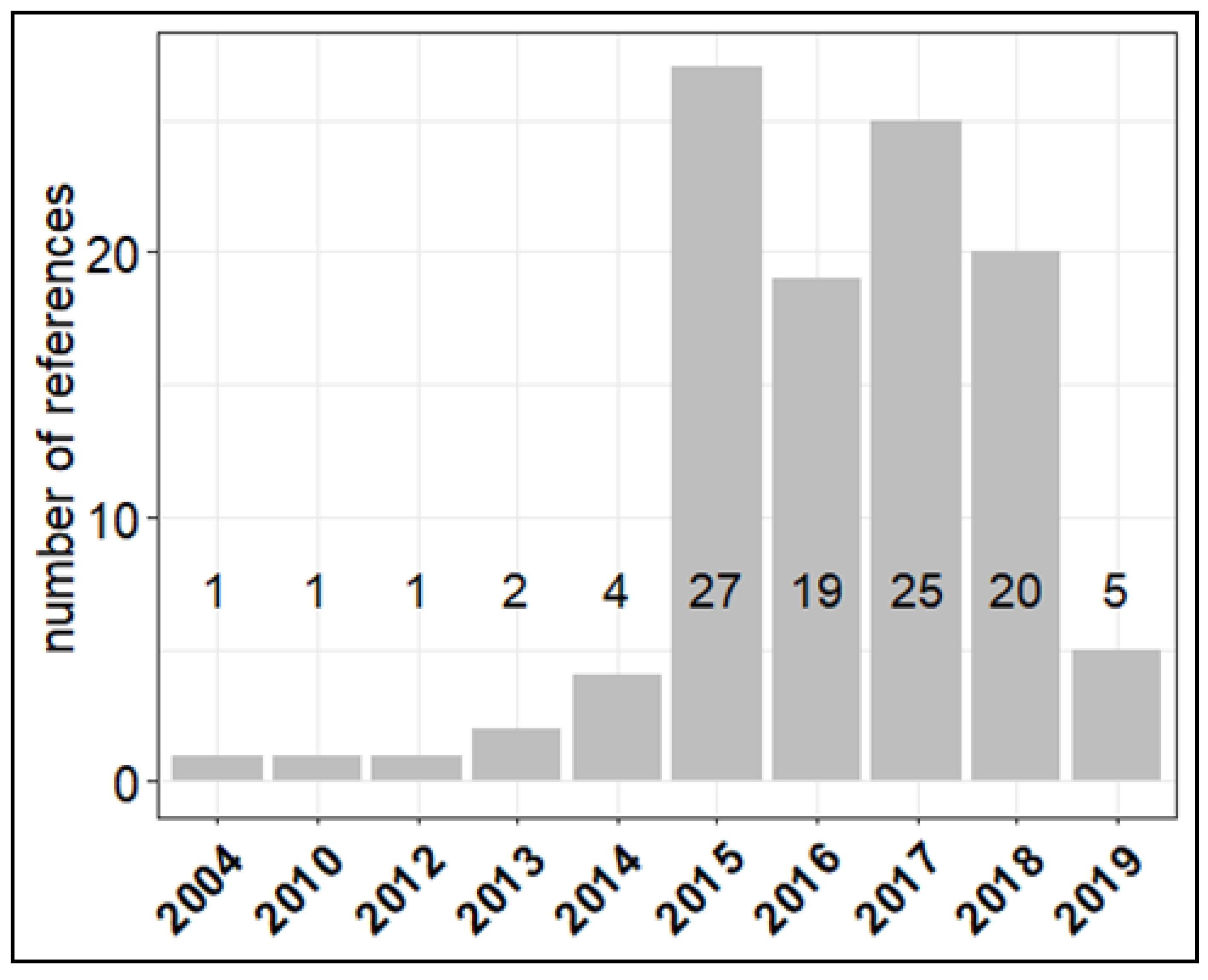
The research covered the period between 2010 and 2019 (year of publication). As shown in Figure 2, only a few preliminary studies on the evaluation of performance of LCS were published between 2010 and 2014. In 2015, we recorded the largest number of references with 27 different works publishing results on performances of LCS for air quality monitoring. For the test studies carried out by AQ-SPEC [19], records were evaluated per model of LCS.
Overall, 34 references reporting field tests with LCS co-located at urban sites were found, as well as 8 references for rural sites, and 10 references for traffic sites. Most of the laboratory and field tests reported hourly data (610 records for 86 models of LCS). We also found 253 records for 40 LCS using daily data and 248 records for 42 LCS using 5-minute averages (Table A1). Therefore, records from hourly data were considered statistically more significant.

3. Method of Evaluation

The European Union Air Quality Directive indicates that measurement uncertainty [88] shall be the main indicator used for the evaluation of the data quality objective of air pollution measurement methods [2]. However, the evaluation of this metric is cumbersome [89,90] and it is not included in the majority of sensor studies (see Table 2). For the performance criteria used to evaluate air quality modeling applications [91], the set of statistical indicators includes the root mean square error (RMSE), the bias, the standard deviation (SD), and the correlation coefficient (R), of which RMSE is thought to be the most explicative one. The statistical indicators can be better visualized in a target diagram [20]. Unfortunately, Table 2 also shows that RMSE is mainly unreportable in the literature. As already mentioned above, integrated indicators, such as the IPI [34], would breach our objective to use solely quantitative and comparable indicators. Additionally, it is impossible to compute IPIs a posteriori, since time series are mainly not available in literature.
Therefore, we had to rely on the most common metrics, i.e., the coefficient of determination R2 and the slope and intercept of the linear regression line between LCS data and the reference measurement. R2 can be viewed as a measure of goodness of fit (how close evaluation data is to the reference measurements) and the slope of the regression as the level of accuracy. R² measures the strength of the association between two variables but it is insensitive to bias between LCS and reference data—either relative bias (slope different from 1) or absolute bias (intercept different from 0). R2 is a partial measure of how much LCS data agree with reference measurements according to a regression model [92]. A larger R2 reflects an increase in the predictive precision of the regression model. The majority of the reviewed works reported R2 value as a main metric when comparing LCS with reference measurements. Table 2 clearly shows that only a few records were found for the measurements reporting mean absolute error (MAE), bias, and RMSE [42,49,52,53,54,56]. However, we would like to stress that other statistical parameters, such as the mean normalized bias (MNB), mean normalized error (MNE), and the root mean square error (RMSE), are also very important in evaluating the relationship between LCS and reference instruments.
An increase of R² may not be the result of an improvement of LCS data quality, since R² may increase when the range of reference measurements increases [93] or according to the seasonality of sampling reported in different studies. Because of the different time ranges and seasonality reported in the reviewed records, it was not possible to have a homogeneous dataset with the same meteorological trends and conditions. This might represent a limitation of the present work and could be an element to improve future LCS comparison for the characterization of their calibration performances. Moreover, since LCS are affected by long time drift and ageing, longer field studies are more likely to report lower R² than shorter ones.
Nearly all published studies report the coefficient of determination (R²) between reference and LCS data (see Table 2). Fortunately, the majority of these studies also report the slope and intercept of the regression line between LCS data and reference measurements that describe the possible bias of LCS data. A few studies also report the RMSE [10,20,22,36,41,42,43,51,52,58,60,62,63,85] which clearly indicates that the magnitude of the error in LCS data is also sensitive to extreme values and outliers. Only a few studies report the measurement uncertainty [10,22,25,30,48,52,59,61]. Therefore, for the purpose of this work, we only focused on the analysis of the comparison of laboratory and field tests of LCS.
Table 2 also gives the R² of calibration that was found in the literature. Generally, these studies also present the model equations used for calibration. The number of studies reporting the R² of calibration represents about 10% of the studies reporting R² of comparison of calibrated LCS and reference data using linear regressions.
Although the data set of R² for calibration is limited in size, we have investigated if the type of calibration has an influence on the agreement between calibrated LCS data and reference measurements.
In order to estimate the efficiency of calibration models, the reported coefficient of determination R2 was used as an indicator of the amount of total variability explained by the model (see calibration of LCS). This can be used as an indication of performance of the calibration model chosen to validate the LCS against a reference system.
Using the highest R² of comparison together with the slope of the comparison line near to 1.0, a shorter set of best performing LCS will be drawn together with their sensor technology. It was decided to drop the analysis of intercepts differing from 0, accepting that LCS may produce unscaled data with bias provided that LCS data would vary in the same range as reference measurements due to the slope being close to 1. In any case, the extent of deviation from 0 of the intercepts did not contribute significantly to the bias of LCS data for the best performing LCS as shown in Section 5 and in Appendix A.

4. Evaluation of Sensor Data Quality

4.1. Calibration of Sensors

The method used for the calibration of LCS is generally considered confidential information by the majority of LCS manufacturers and little information can be found about the calibration of LCS that fall under the category “black box” compared to the ones that fall under the category “open source”. In fact, several studies can be found on the calibration of “open source” LCS, both with laboratory and field tests. Calibration consists of setting a mathematical model describing the relationship between LCS data and reference measurements. However, most of the calibrations were carried out during field tests, while only a limited number of laboratory based calibration experiments were found.
Out of a total of 1423 records in the database, 352 records (25%) included information about LCS calibration giving details of used statistical or deterministic models (see Table 3). However, among these 352 records with details of the calibration method, about 20% do not report R², that is, the principal metrics used for LCS performance evaluation. This is typically the case for artificial neural networks, random forest, and support vector regression calibration methods (see below), and it explains why the number of R² found for calibration in Table 2 is lower than 352.
The linear model and the multi-linear regression model (MLR), which includes the use of covariates to improve the quality of the calibration, are the most widely used techniques to calibrate the LCS data against a reference measurement. Other calibration approaches use the exponential, logarithmic, and quadratic methods, the Kohler theory of particle growing factor, and several types of supervised learning techniques, including artificial neural networks (ANN), random forest (RF), support vector machine (SVM), and support vector regression (SVR). Most of the MLR models use covariates such as meteorological parameters (temperature and relative humidity) and cross-sensitivities from gaseous interferents, such as NO2, NO, and O3, in order to improve LCS calibration. LCS data time-drift was rarely included in the list of calibration covariates [39,62]. Several works have demonstrated how electrochemical and metal-oxides LCS are dependent on temperature, humidity, and other gaseous interferent compounds. This dependency is related to the physico-chemical properties of the sensors according to the type of electrolyte, electrode, or semiconductor material used in the sensor; it is not repeated here since it can be found in the literature [97,98,99]. LCS used for the detection of PM are sensitive to the effect of relative humidity. As explained below, relative humidity larger than 70–80% contributes to particle growth with consequent erroneous reading of the particulate number counts. One of the solutions for this shortcoming consists of implementing a theory for the growth of particulates due to humidity when converting particulate numbers into mass concentrations [48,84,96].
When R² is both available for calibration and comparison, the median of R² is higher for calibration (mean of R² = 0.70) than for comparison (median of R² = 0.58). This is to be expected, as it is easier to fit a model on a short calibration dataset than correctly forecast LCS data using the calibration model at later dates. For gaseous LCS, calibration using a linear model was shown to be the worst R² for field comparison (see Table 3). Therefore, linear calibration should be avoided for gas LCS.
For CO and NO, we observed that the calibration method giving the highest R² (about 0.90) is the MLR method using temperature or relative humidity as covariates. The use of supervised learning techniques (ANN, RF, or SVR) either did not improve performance for CO or gave similar results as MLR for NO. This is in slight contradiction with other studies on the performance of supervised techniques [100,101]. In the majority of cases, these tested LCS consisted of electrochemical sensors. Only for NO2 did we observe that supervised learning techniques (ANN, RF, SVM) performed slightly better than MLRs when looking at the R² of comparison tests in the field, except for SVR, which is in slight contradiction with other studies [101]. However, the number of records is much higher for MLR than for supervised learning techniques. MLR was applied to both MOs and electrochemical sensors, which resulted in scattered R² when looking at individual studies. Additionally, supervised learning techniques may be more sensitive to re-location than MLR [86,87].
For O3, ANN and MLR calibration gave similar R² of comparison (median value about 0.90). As for NO2, the higher number of studies makes the R² of the MLR method more significant than the one for ANN.
In general, all machine-learning techniques are able to account for multiple and unknown effects resulting in a more accurate prediction of the outputs based on training data and depending on the correctness of the list of input parameters. For CO, the lower R² values of the ANN calibration method were likely caused by an incorrect choice of input parameters. For O3 and NO, the R² values were already high (about 0.9, as indicated in the manuscript) for both MLR and supervised learning techniques, leaving little room for improvement using supervised learning techniques. For NO2, the higher R² values when calibrating with supervised learning techniques likely came from using O3 as input parameters, a quantitative interferent for electrochemical NO2 sensors. The ratio of O3/NO2 distinguishing the type of field site often has a direct influence on the performance of electrochemical NO2 sensors.
For PM, the R² for comparison tests are very scattered over the calibration methods. Some high values (R² higher than 0.95) were reported for studies using a linear calibration, while MLR did not perform well (R² < 0.5). These results are misleading, since the good results with linear calibration are generally obtained by discarding LSC data obtained with relative humidity exceeding a threshold between 70 and 80%, above which humidity is responsible for particle growth [84,96]. This effect is more important for PM10 than for PM1 and PM2.5. Other studies did not discard high relative humidity, they took into consideration the particle growth factor, either on mass concentration with an exponential calibration model ([73,75,82]) with a median R² of 98 or using the Kölher theory on PM mass concentration [80], or directly for the particle beans of each OPC bin [96], leading to R² of about 0.80.
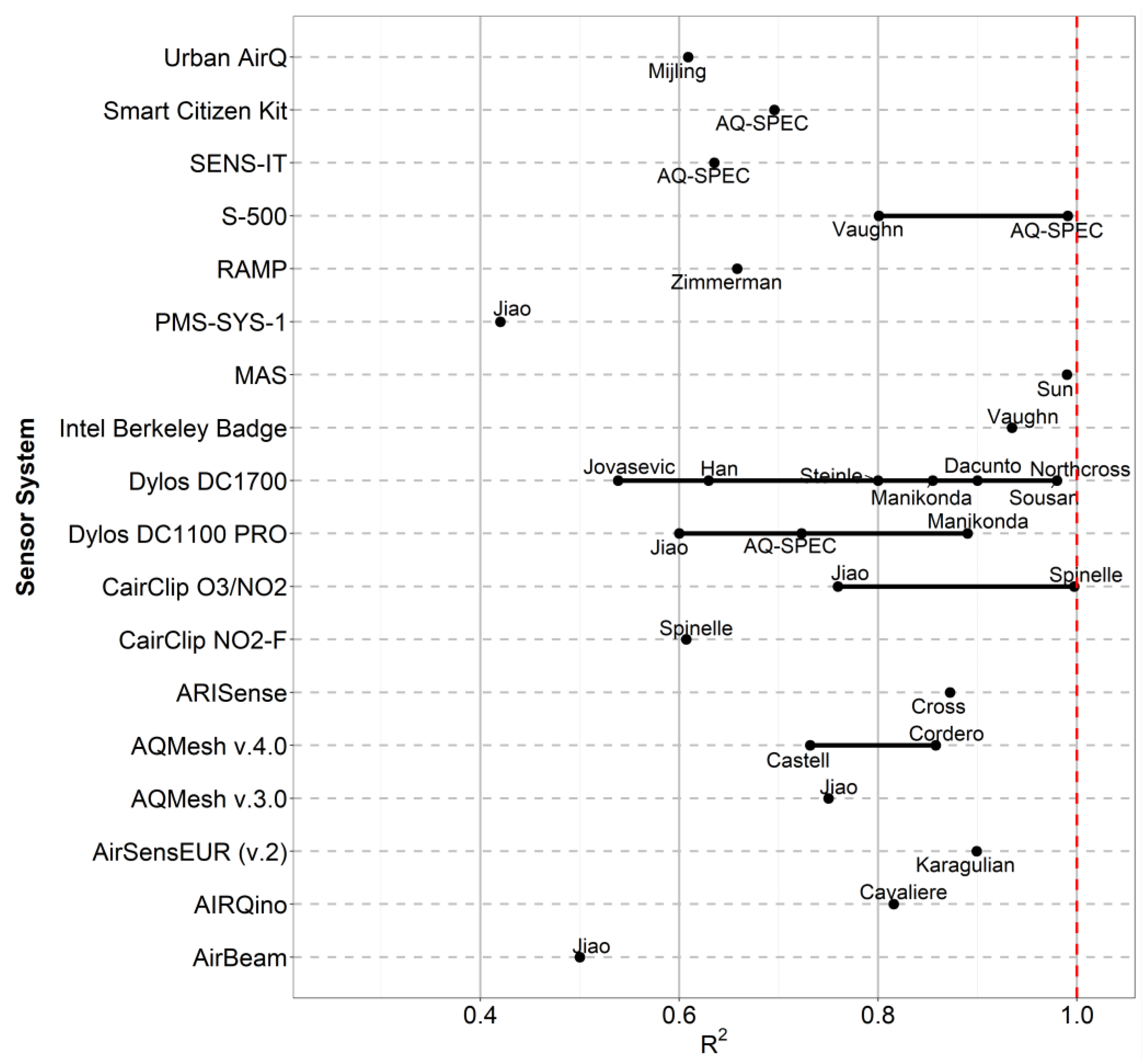
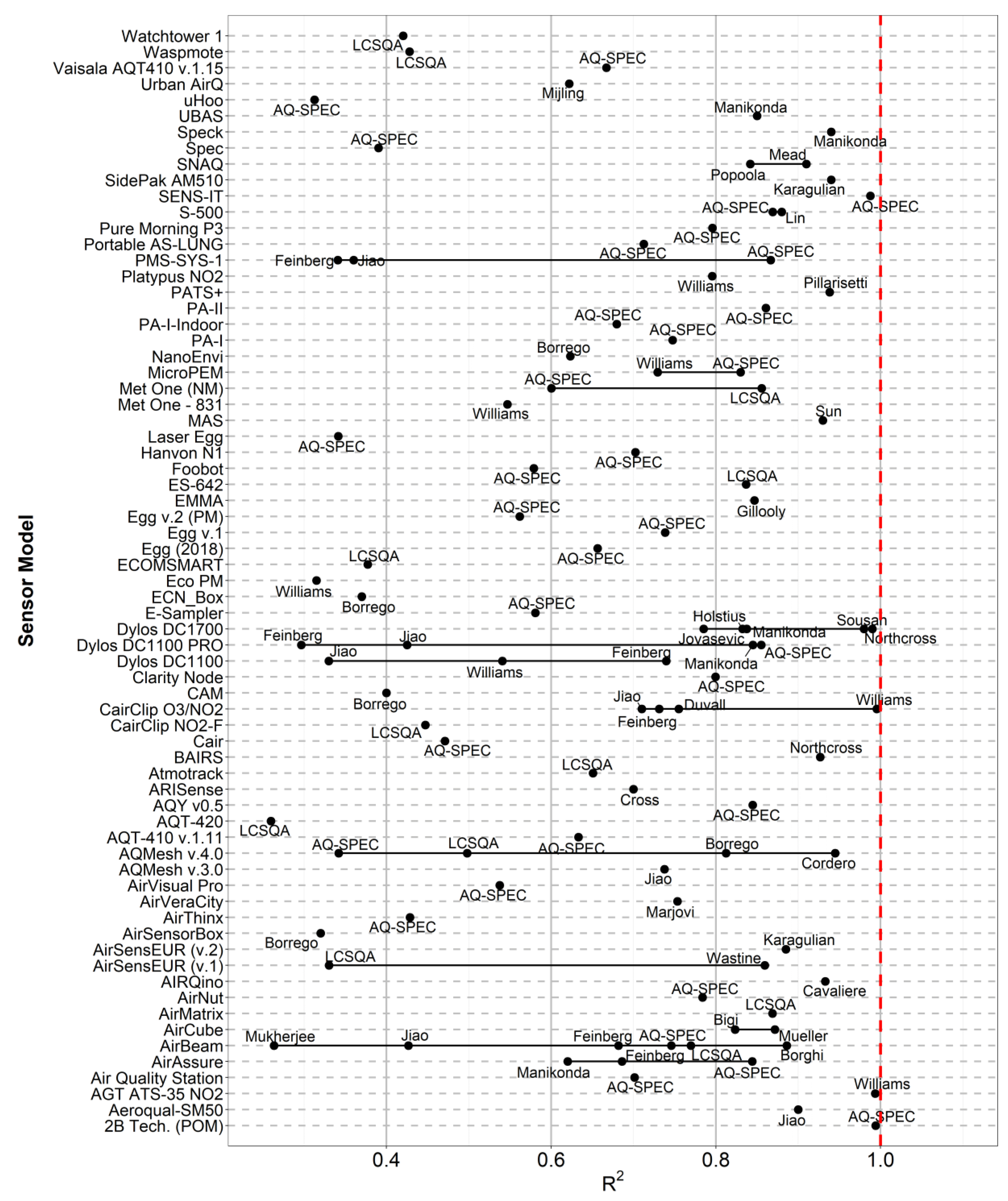
Figure 3 shows a summary of all mean R2 obtained from the calibration of SSys against reference measurements. Results were grouped by model of SSys and averaged per reference work. For the same SSys we can observe R2 ranging between 0.40 and 1.00. This shows the variability of the performance of SSys depending on the type of calibration, type of testing sites, and seasonality, making it difficult to compare the results of the different studies.
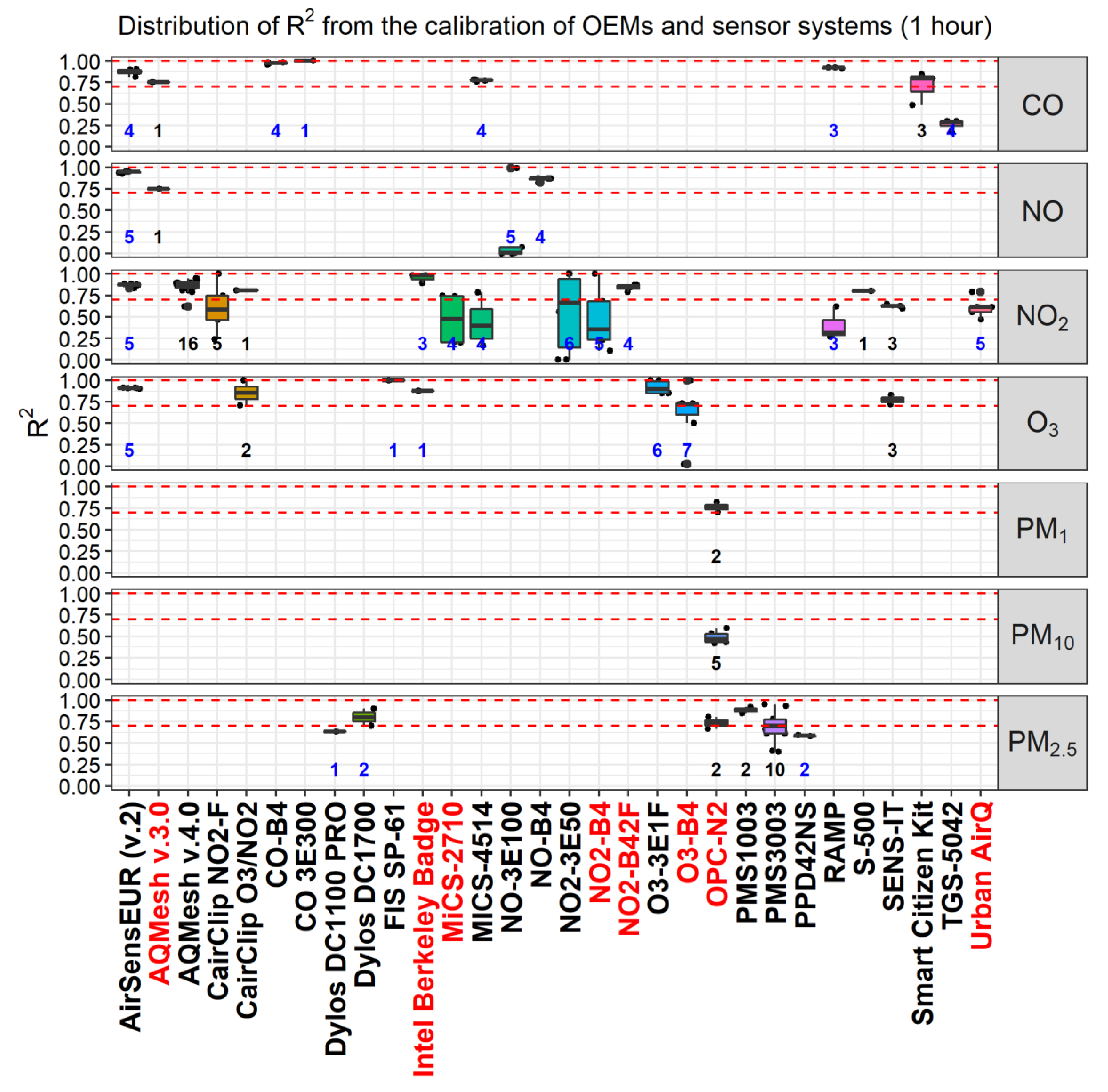
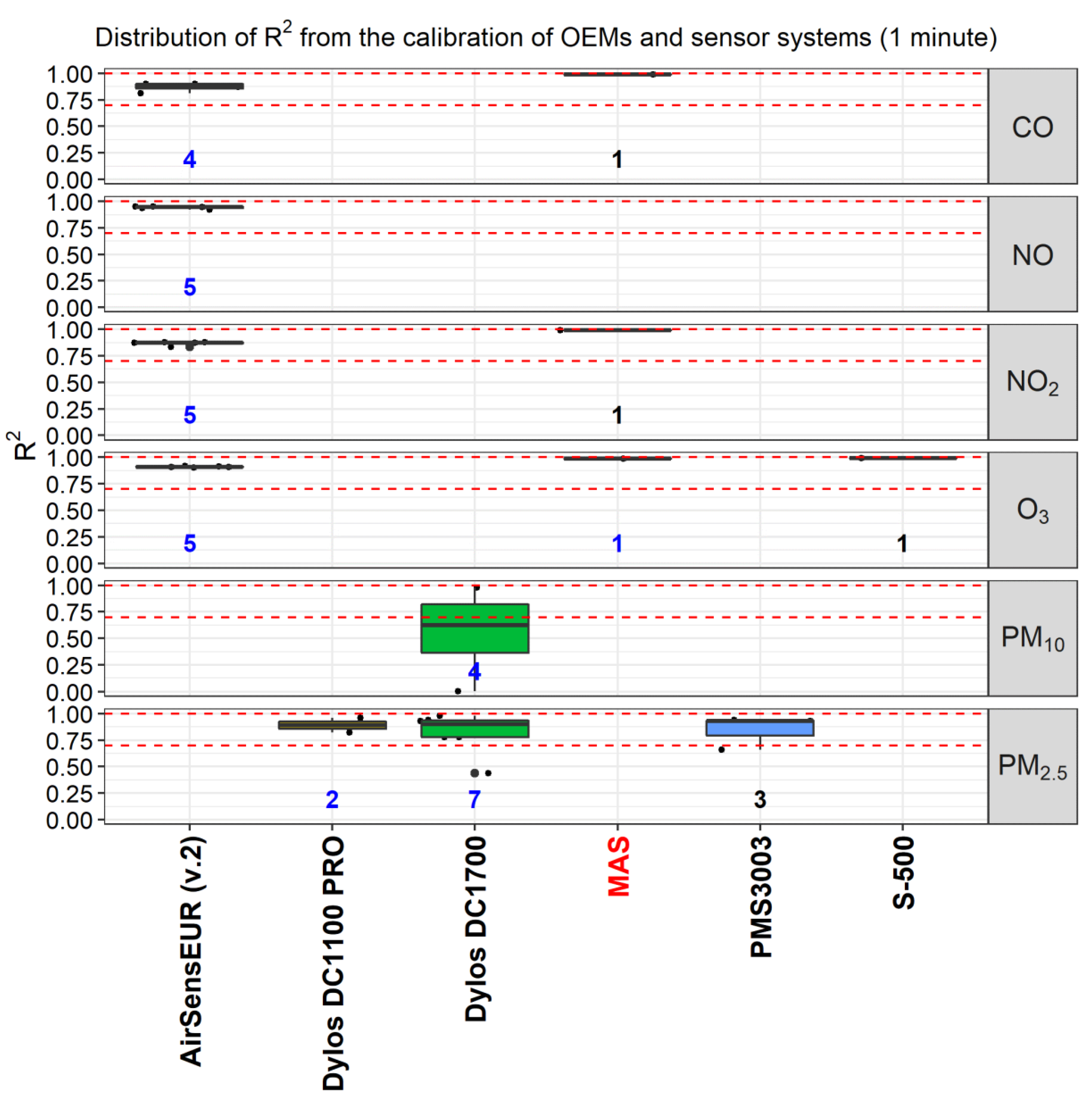
Calibration of LSC against a reference analyzer was found to be carried out using different averaging times. Test results with hourly data are presented in Figure A1 and test results with minute data time are given in Figure A2.
The best performance, according to the time average availability in the literature and tests in the laboratory or in the field, were as follows:
  • For the measurement of PM2.5, values of R2 close to 1 were found for hourly data of PMS1003 and PMS3003 by Plantower [75] DC1100 PRO and DC1700 by Dylos (Riverside, USA) for minute data [14,19,79]. Strangely, higher R2 were reported for the Plantower and Dylos when calibrated with minute data than for hourly data. The OPC-N2 by AlphaSense [19] reported values of R2 falling within the range of 0.7–1.0. The same OPC-N2 reported values of R2 just above 0.7 when measuring PM1, while it did not show a good performance when measuring PM10 [19] (R2 less than 0.5). We need to stress that optical sensors, such as OPCs and nephelometers, are somewhat limited in coping with gravity effects when detecting coarse PM because of the low-efficiency of the sampling system. Most of the regression models used for the calibration of LCS used hourly data.
  • For the calibration of O3 LCS, the highest values of R2 for hourly data was reported for FIS SP-61 by FIS (Osaka, Japan) and O3-3E1F [20] by CityTechnology (Figure A1) (Portsmouth., UK). On the other hand, for minute data, values of R2 close to 1 were found for AirSensEUR (V.2) [22] by LiberaIntentio (Malnate, IT), as well as for the S-500 [19] by Aeroqual (Figure A2) (Auckland, NZ). AirSensEUR used a built-in AlphaSense OX-A431 OEM. We want to point out that most of the MLR models used to calibrate O3 LCS need NO2 to correct for the strong NO2 cross-sensitivity.
  • For the calibration of NO2 LCS, we found values of R2 for hourly data within the range of 0.7–1.0 for the NO2-B42F [59] (by Alphasense), for the AirSensEUR (v.2) [22] by LiberaIntentio, and for the minute values of MAS [40] (see Figure 3). The NO2 measurement by AirSensEUR (v.2) is carried out using the NO2-B43F OEM by AlphaSense.
  • Most of the records of the calibration of CO LCS showed high values of R2. As shown in Figure A1, the OEMs CO 3E300 [23] by City Technology and CO-B4 [59] by Alphasense reported R2~1 for hourly data. High values of R2 were also reported for the SSys AirSensEUR (v.2) when calibrating CO minute data [22] (Figure A2). Other LCS reporting values of R2 within the range of 0.7–1.0 for hourly data consisted of the MICS-4515 [62] by SGX Sensortech (Corcelles-Cormondreche, CH), the Smart Citizen Kit [19] by Acrobotic (https://acrobatic.com), and RAMP [61].

4.2. Comparison of Calibrated Low-Cost Sensors with Reference Measurements

In this review, records describing the comparison of LCS data with reference measurements came from “open source” and “black box” LCS. As for the records collected from the calibration of LCS, comparison with reference systems was carried out at different time-resolutions. Here, we only report comparisons of hourly data with 565 and 151 records from SSys and OEMs, respectively. In Figure 4, we show the R2 values for SSys per reference averaged for all pollutants measured by each SSys. One can observe scattered R2 for a few SSys that are tested in several references in different locations, seasons, and durations.
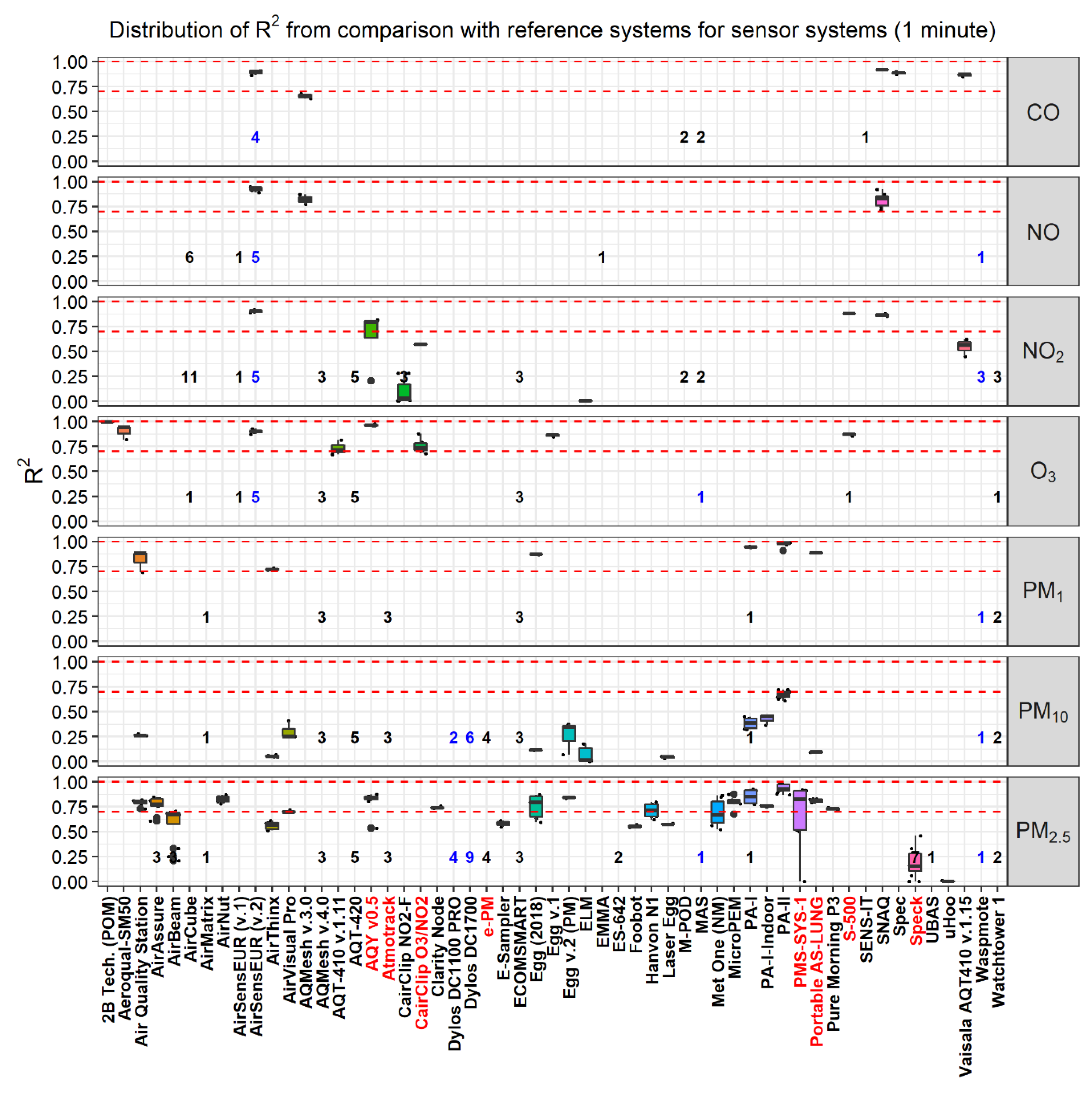
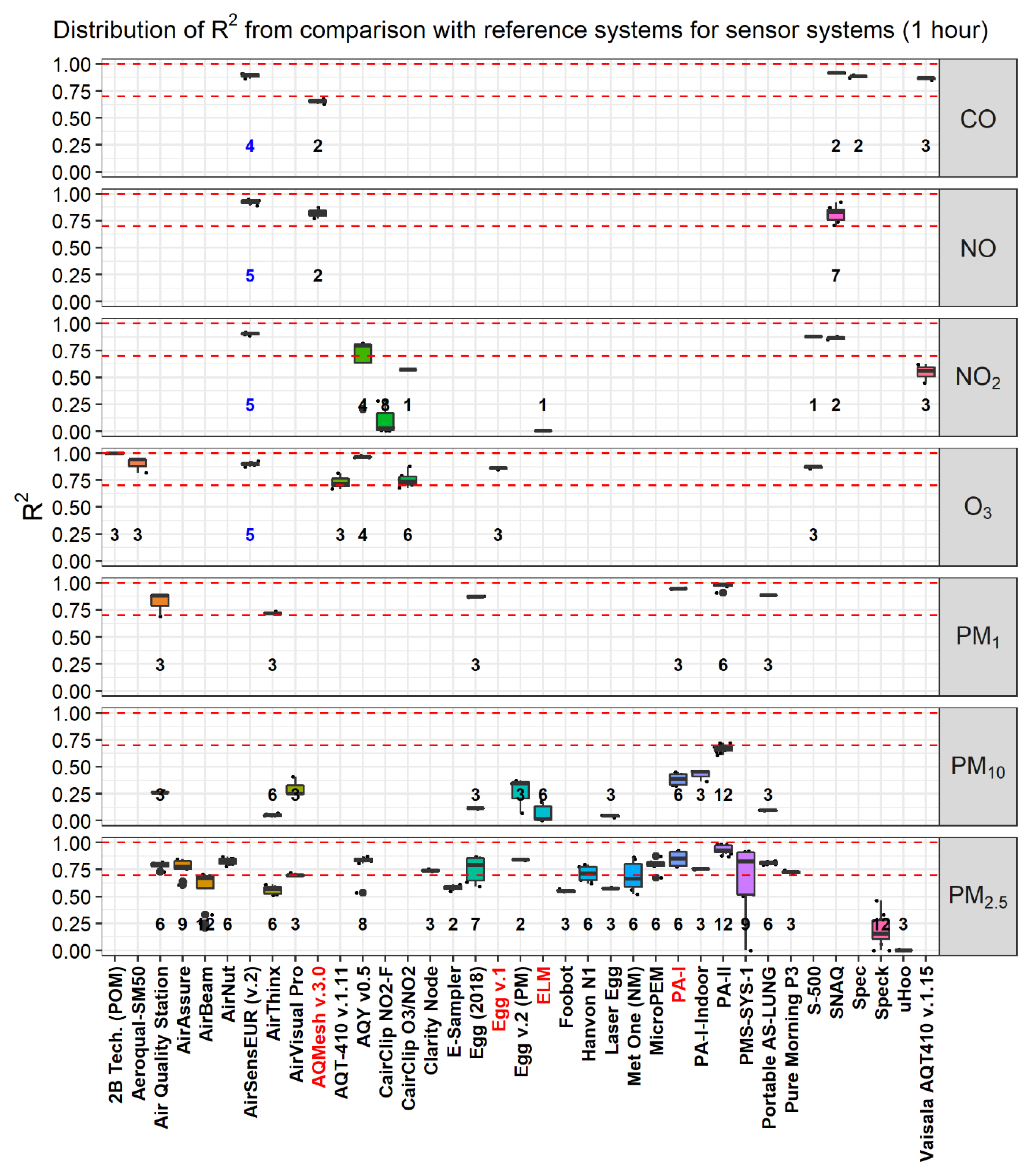
Figure A3 and Figure A4 show the distribution of R2 of LCS hourly and minute values measuring PM10, PM2.5, PM1, O3, NO, NO2, and CO against reference measurements:
  • For the SSys, PA-II by PurpleAir [19] and PATS + by Berkley Air [72] showed the highest R² with values between 0.8 and 1.0. Other LCS with R2 values ranging between 0.7 and 1.0 included PMS-SYS-1 by Shinyei (Kobe, JPN) , Dylos 1100 PRO by Dylos, MicroPEM by RTI (Research Triangle Park, USA), AirNUT by Moji (Beijing, CN), the Egg (2018) by Air Quality Egg (https://airqualityegg.com/home), AQT410 v.1.15 by Vaisala (Helsinki, Finland), AirVeraCity by AirVeraCity (Lausane, CH), NPM2 [33] by MetOne (Grants Pass, OR, USA), and the Air Quality Station [19] by AS LUNG. Nevertheless, we need to point out that the performance of LCS measuring PM10, on average, was very poor.
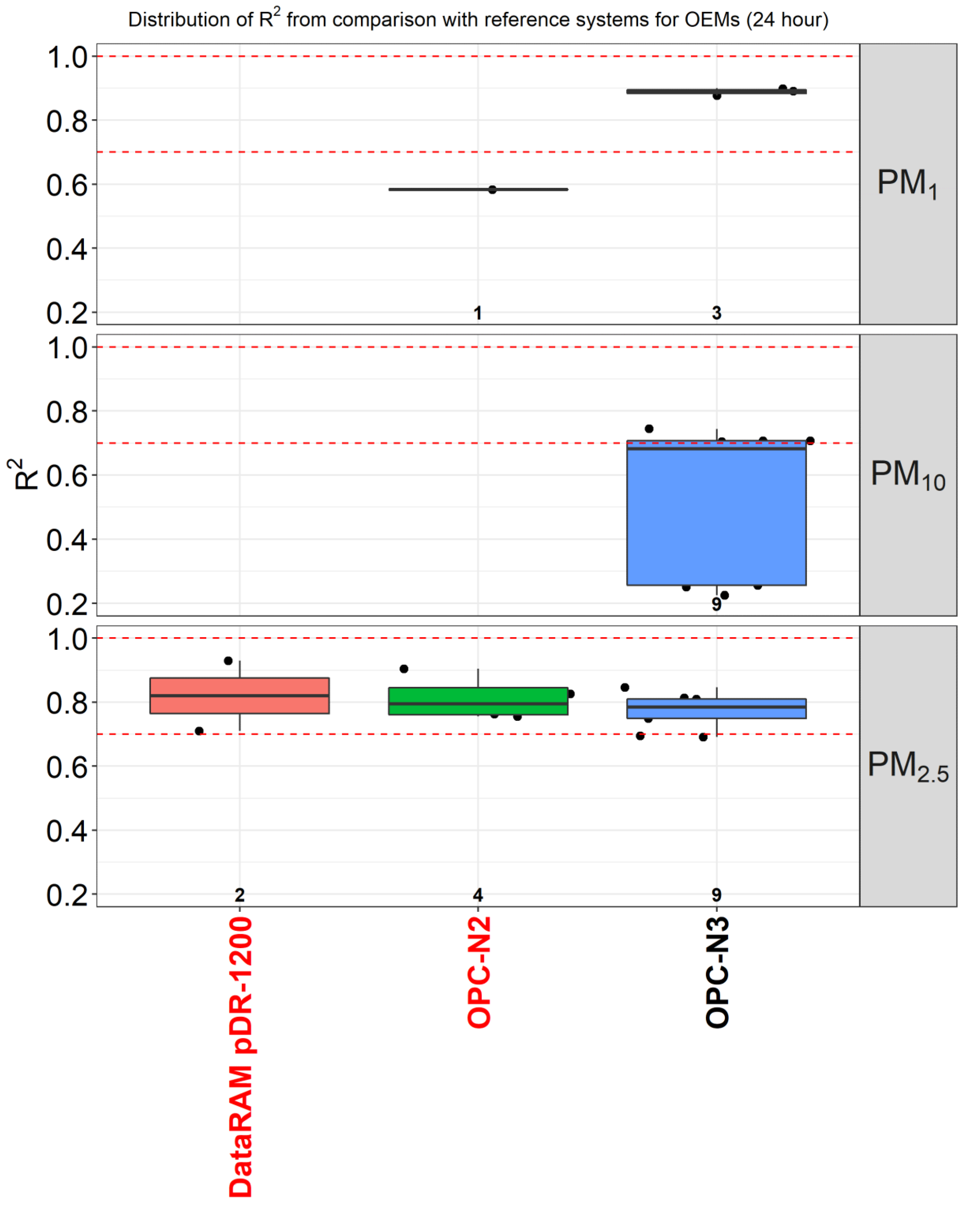
  • For the hourly PM measurements of OEMs (Figure A5), the OPC-N2, OPC-N3 [19,35,36,49,84] and the SDS011 [49] by Nova Fitness (Jinan, CN) showed R2 values in the range of 0.7–1.0. For the 24-hour PM measurements of OEMs (Figure A6), we found R2 within the range of 0.7–1.0 for the OPC-N2 and the OPC-N3 [19].
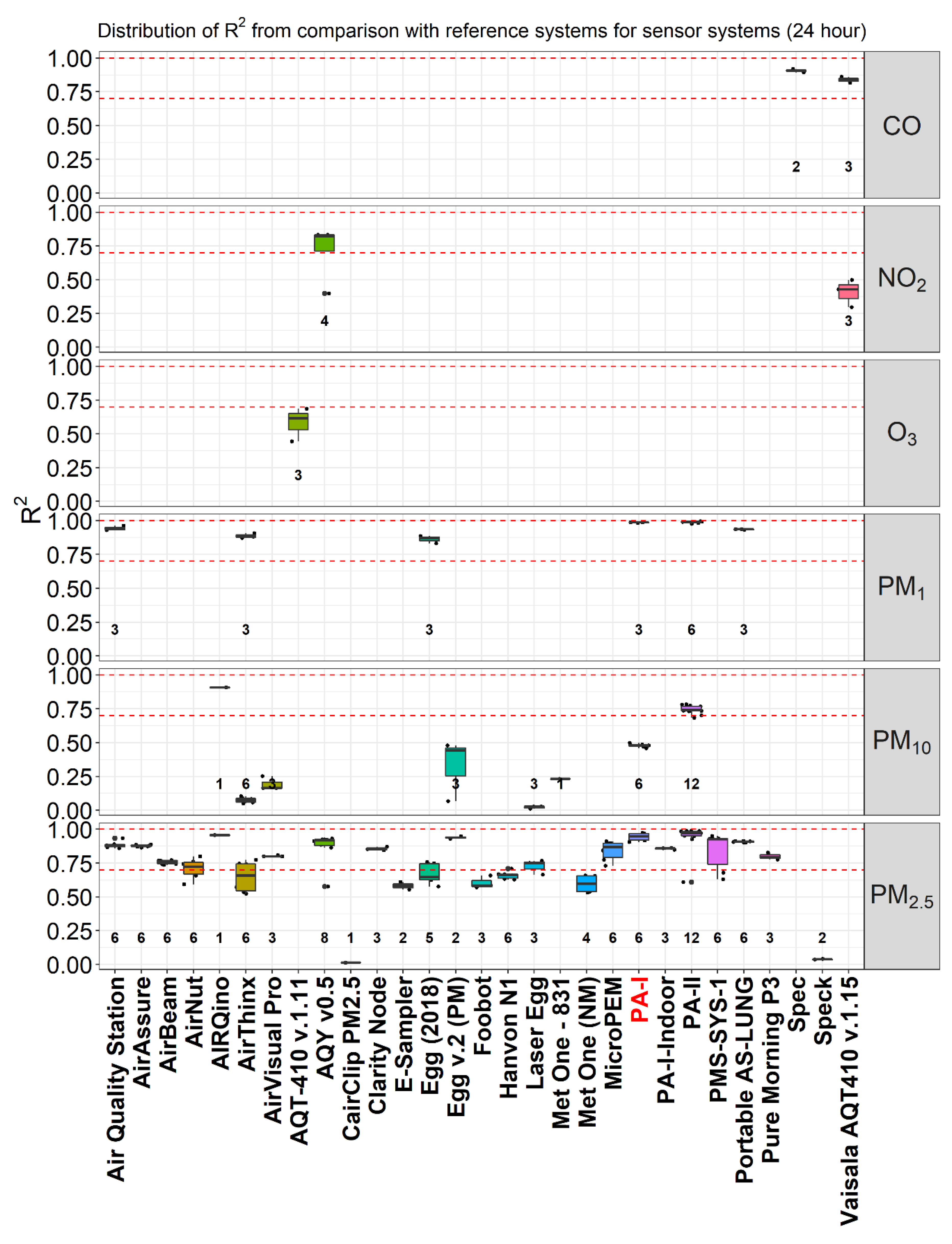
  • For the 24-hour PM measurements of SSys (Figure A7), PA-II [19] and AirQUINO [76] by CNR (Firenze, IT) showed R2 values close to 1 for PM2.5
  • For gaseous pollutants, high R2 values ranging between 0.7 and 1.0 were found for the following multipollutant LCS: AirSensEUR [22] by LiberaIntentio, AirVeraCity, AQY and S-500 by Aeroqual, and SNAQ by the University of Cambridge (Cambridge, UK) (Figure A3).
  • For the hourly gaseous measurements (Figure A5), we found very few OEMs with R2 in the range of 0.7–1.0. These included CairClip O3/NO2 [20,30,36,64] by CairPol (Poissy, France), Aeroqual Series 500 (and SM50) [33] and O3-3E1F [20,23,36] by CityTechnology, and NO2-B43F [61,65] by Alphasense. On the other hand, we found very few records for SSys using daily data. Additionally, one can notice when comparing Figure A4 and Figure A5 that the performance of OEMs is generally enhanced when they are integrated inside SSys, except for PM10.
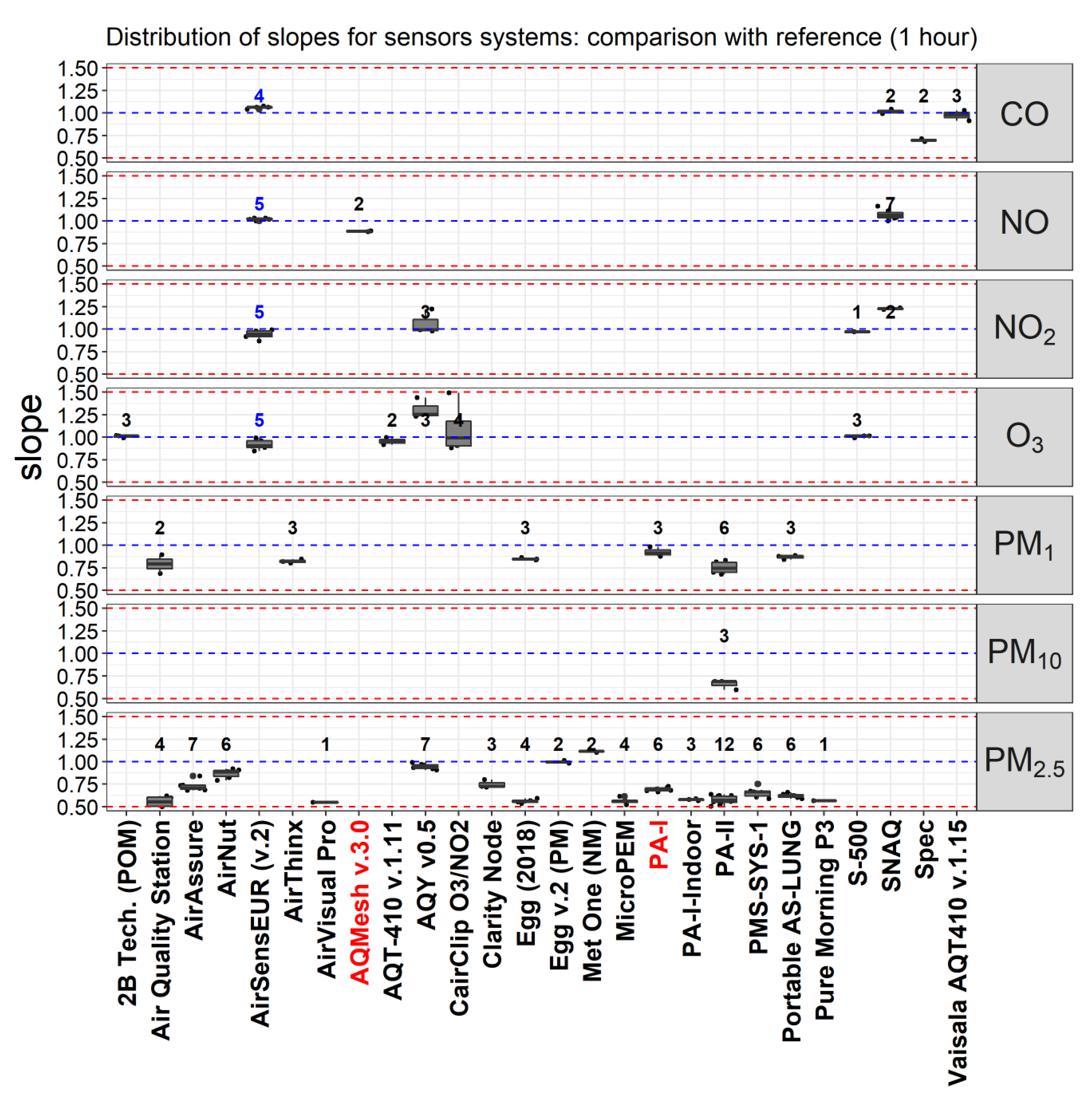
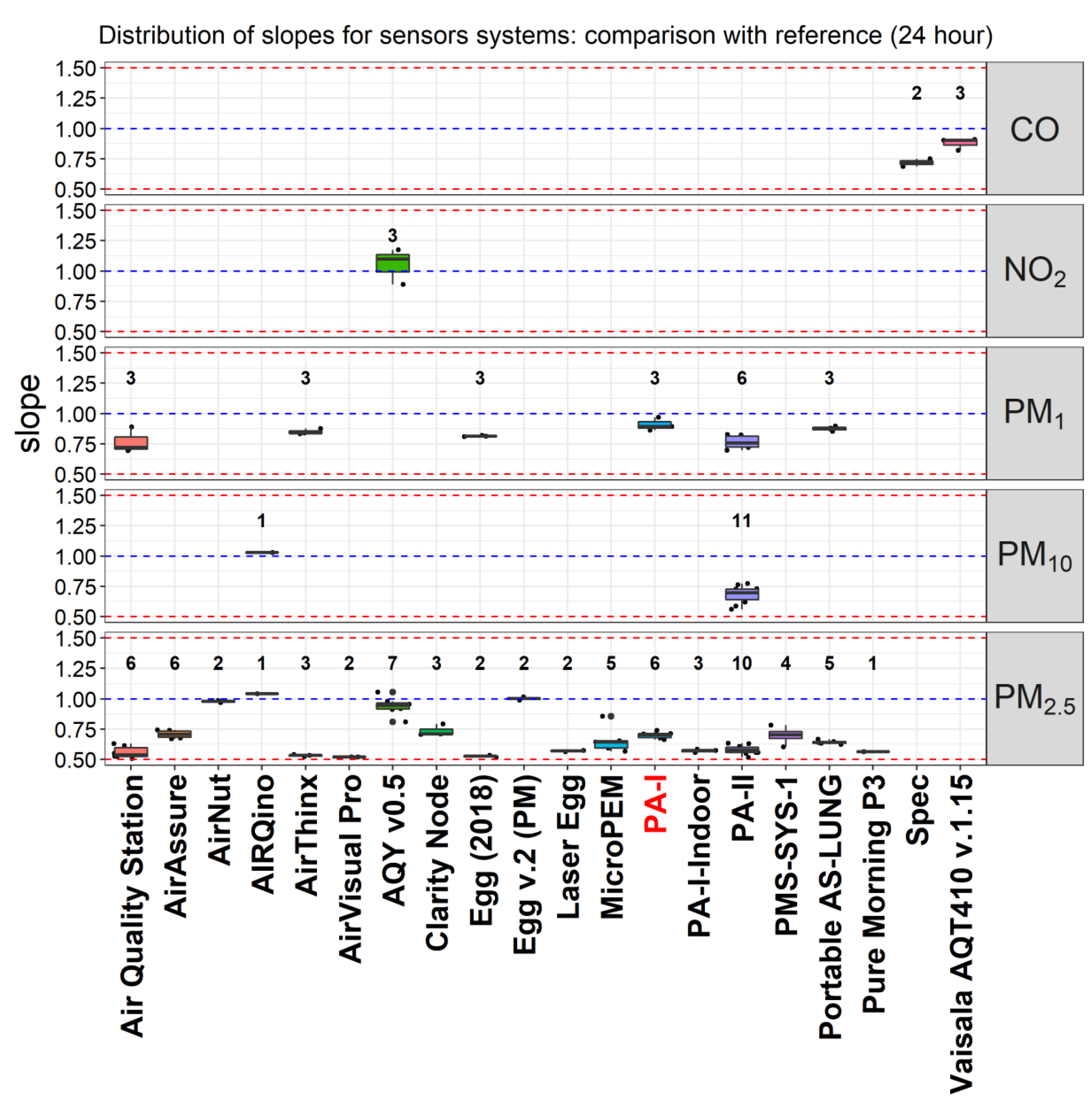
Figure A8 and Figure A10 show selected SSys that gave the slope of the linear regression line of hourly LCS data versus reference measurements from 0.5 to 1.5 and R² higher than 0.7. This selection includes AirSensEUR, AirVeracity, and S-500 for gaseous pollutants and AirNut, AQY v0.5, Egg v.2 (PM), NPM2 for hourly data and AIRQuino, AQY v0.5, Egg v.2 (PM), and PA-I for daily data.
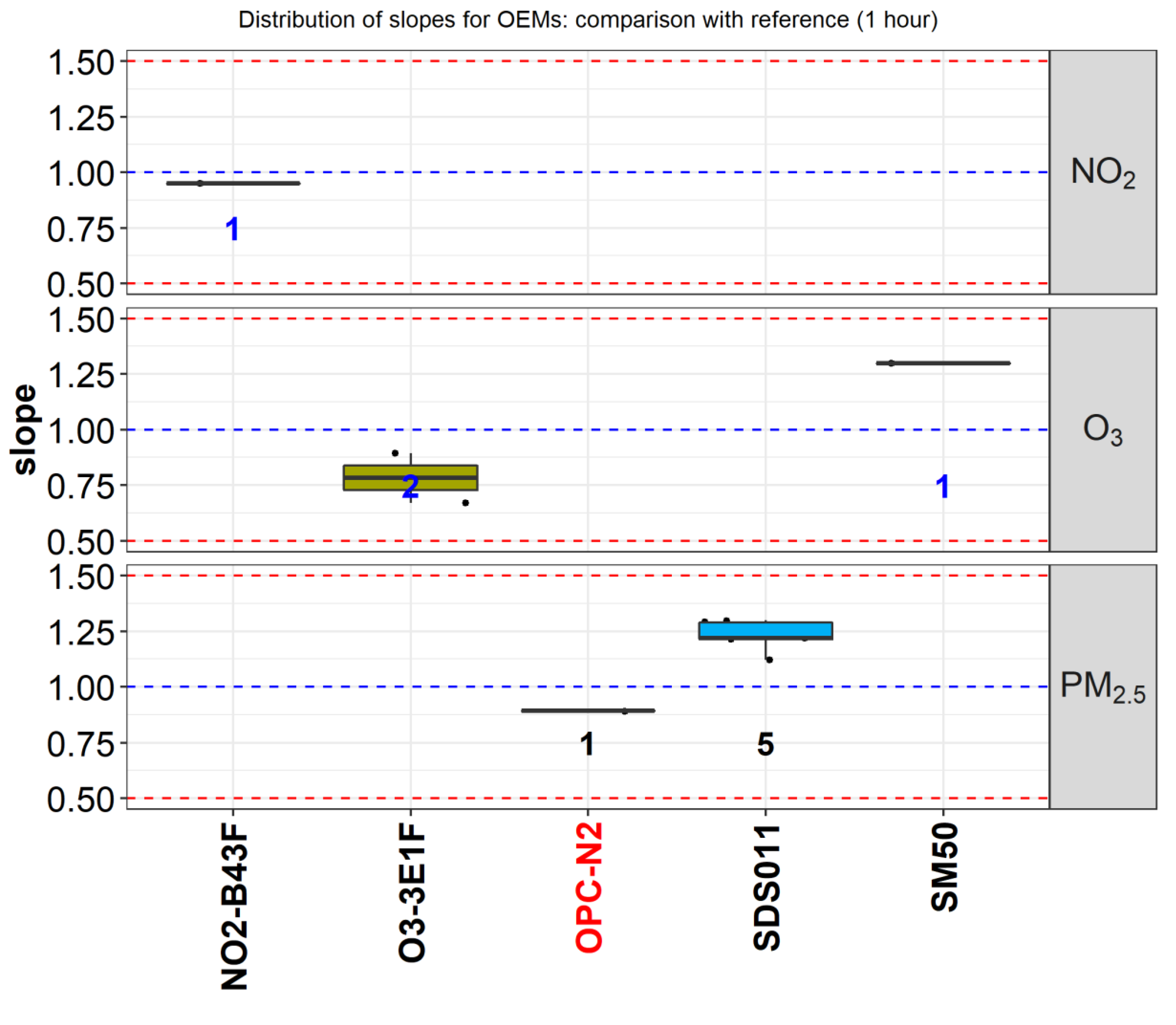
Figure A9 and Figure A11 show the same selection as Figure A8, but for OEMs. This list includes the SM50, CairClip O3/NO2, S-500 (NO2, O3), and NO2-B4F (NO2) for gaseous measurements, Nova Fitness SDS011 for PM2.5 measurements for hourly data, and the OPC-N2 by Alphasense and DataRAM for daily data.
The influence of the type of reference methods was evaluated by plotting the R2 of sensor data versus reference measurements. In total, 657 of the studies used GRIMM Environmental Dust Monitor (Airing, GE) (58%), Beta Attenuation Monitor (BAM) (36%), DustTrack (<1%), and Aerodynamic Particle Sizer (<1%), all based on light scattering, the same principle as PM sensors. Other studies used the Tapered Element Oscillating Microbalance method (TEOM) (5%) and Gravimetry (<1%). The 25%, 50%, and 75% percentiles of R2 were 0.56, 0.78, and 0.91 for GRIMM and 0.41, 0.66, and 0.81 for BAM, respectively. Consequently, it was not possible to identify any significant difference for the two mainly used analyzers (GRIMM, BAM) because of the overlap of the distributions of R2. In fact, the effect of the type of reference method must be considered together with the background conditions at which the comparison is carried out. These conditions might have a non-negligible effect on the PM concentration measured by the sensor, and therefore may influence the value of R2 more than the type of reference measurement. Additionally, the relationship between R2 (obtained from the comparison of LCS with reference instruments) and the maximum reference concentration of each study did not show any trend.

5. Cost of Purchase

For the evaluation of the price of LCS, we considered all SSys manufactured by commercial companies. Operating costs, such as calibration, maintenance, deployment, and data treatment, were not included in the estimated price of SSys.
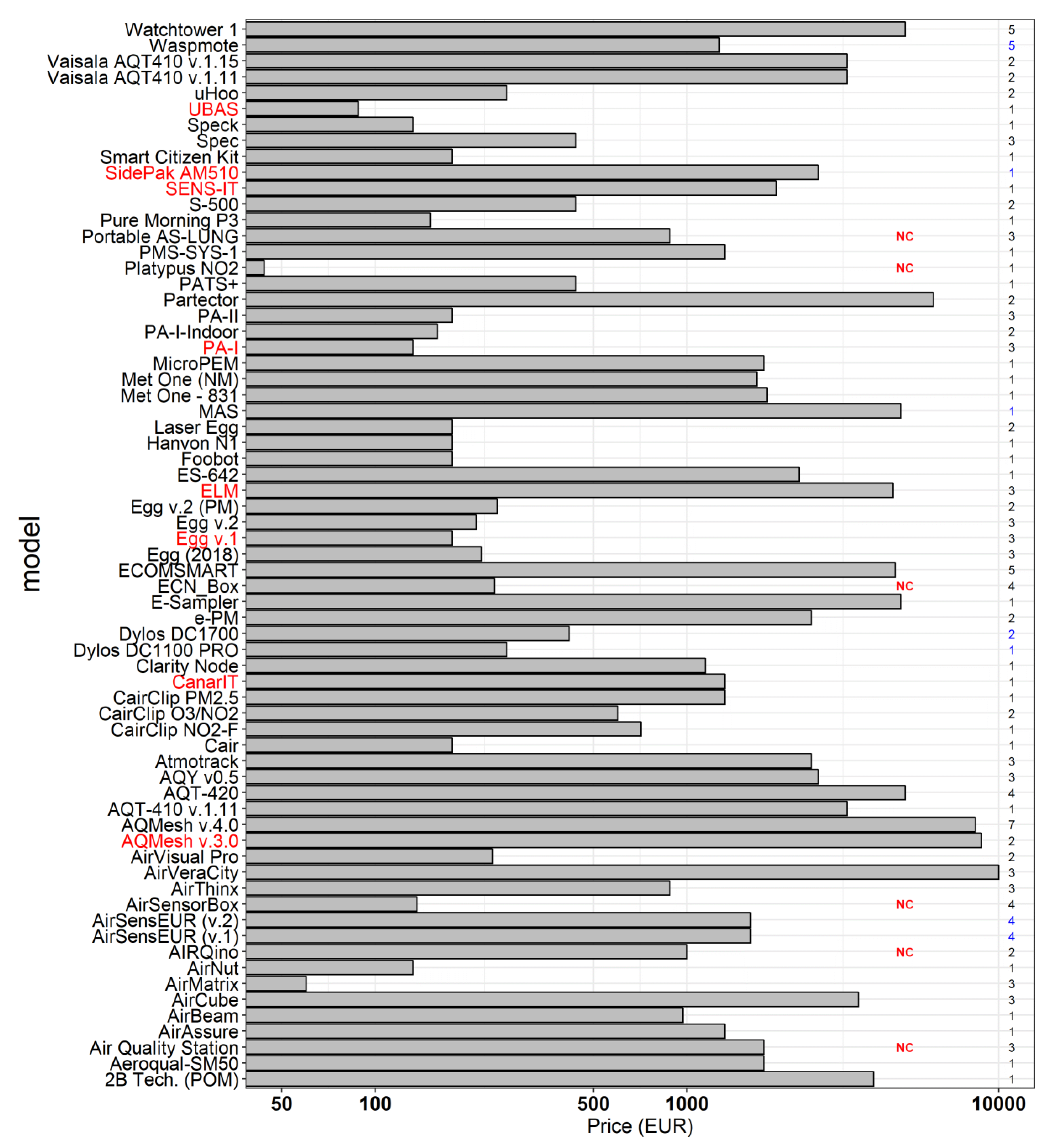
Figure 5 shows the commercial price of LCS by model and number of measured pollutants and Figure A13 shows the prices for OEMs. There are a large number of SSys measuring one pollutant and only a few measuring multiple pollutants. Most OEMs are open source devices (Figure A13). On the other hand, most of the SSys are “black box” devices (Figure 5). Therefore, most of the SSys cannot be easily re-calibrated by users. In fact, most SSys are intended to be ready-to-use air quality monitors.
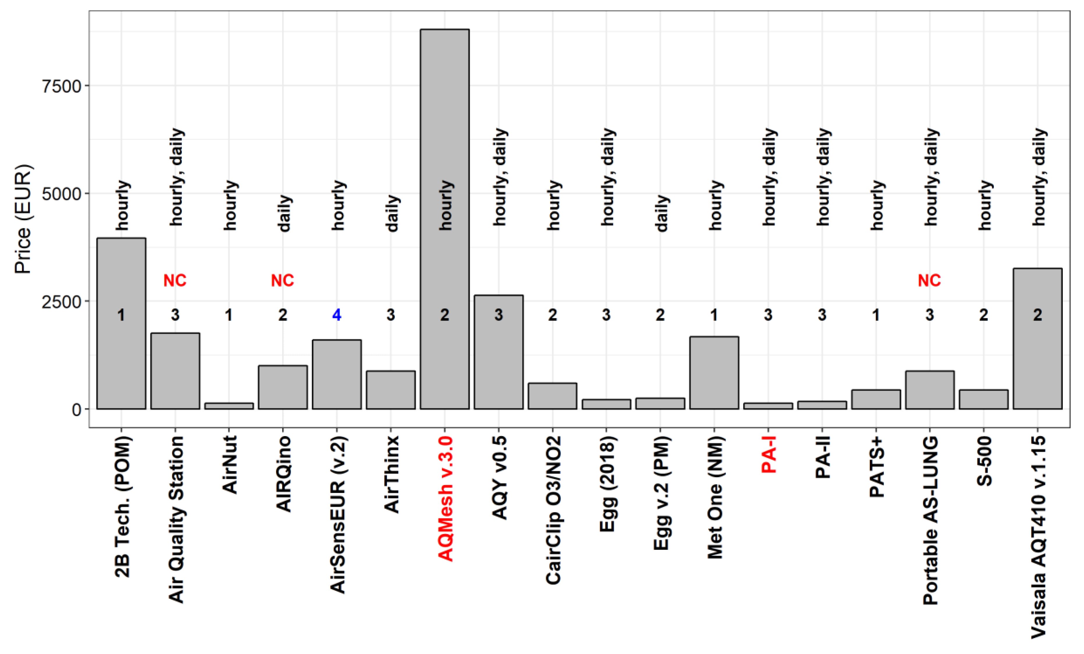
In Figure 6 we have shortlisted the best SSys according to their level of agreement with reference systems. Figure 6 includes SSys with hourly and daily data showing R2 higher than 0.85 and slopes ranging between 0.8 and 1.2. The figure shows the price, the number of pollutants being measured, the averaging time, and the data openness of the selected SSys. Table 4 reports the SSys shortlisted in Figure 6 with the R² and slope mean values, the list of pollutants being measured, the openness of data, their commercial availability, and price.
Among “open source” SSys, we identified the AirSensEUR by LiberaIntentio and the AIRQuino by CNR. The remaining shortlisted SSys were identified as “black box”. AirSensEUR (v.2) resulted in a mean R2 value of 0.90 and a slope of 0.94, while AIRQuino resulted in a mean R2 value of 0.91 and a slope of 0.97. We need to point out that, to date, AIRQuino can be used for the detection of up to five pollutants (NO2, CO, O3, NO, and PM). However, only data for PM were available at the time of this review.
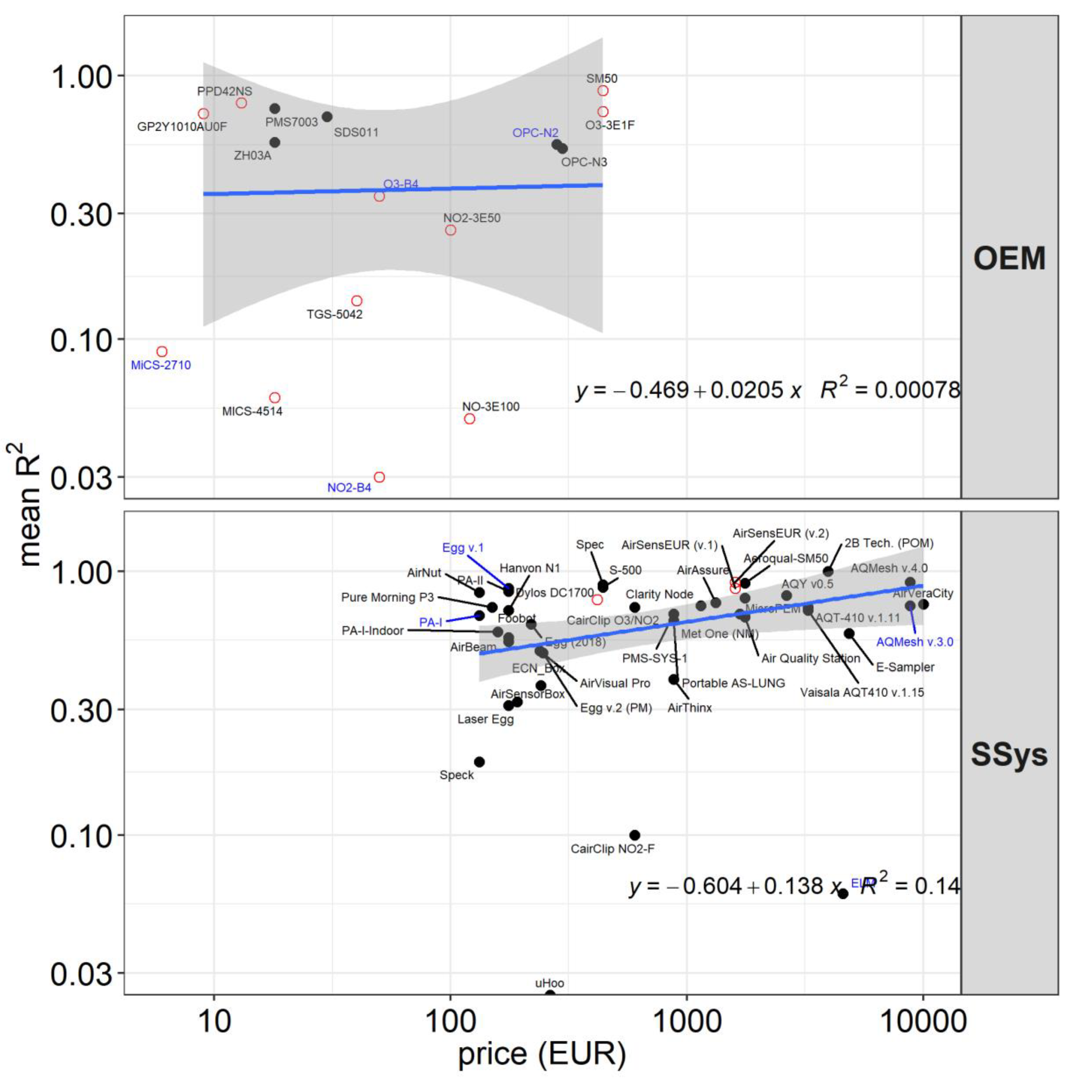
Figure 7 shows the relationship between the mean R2 of SSys and the decimal logarithm of the price of LCS. In Figure 7, only the “living” LCS are compared. This shows that for OEMs there is not a significant linear relationship between the price of OEMs and the value of R2. Conversely, there is a significant increase in R² with the logarithm of the price of SSys. The regression equations indicated in Figure 7 shows that R² can increase 14 ± 6% for a 10-fold increase of the prices of SSys, which is a limited increase at high cost. Figure 7 also shows a higher scattering of R² at the low end of the price scale at SSys price lower than 500 euro, with more fluctuation of the SSys performance.

6. Conclusions

There is little information available in the literature regarding calibration of LCS. Nevertheless, it was possible to list the calibration methods giving the highest R² when applied to the results of field tests. For CO and NO, our review showed that the MLR models were the most suitable for calibration. ANN gave the same level of performance as MLR only for NO. For NO2 and O3, supervised learning models, such as, SVR, SVM (though not for O3), ANN, and RF, followed by MLR models, proved to be the most suitable method of calibration. Regarding PM2.5, the best results were obtained with linear models. However, these models were applied only to PM2.5 with relative humidity data < 75–80%. For higher relative humidity, models accounting for the growth of the particulates must be further developed. So far, the calibration using the Khöler theory seems to be the most promising method.
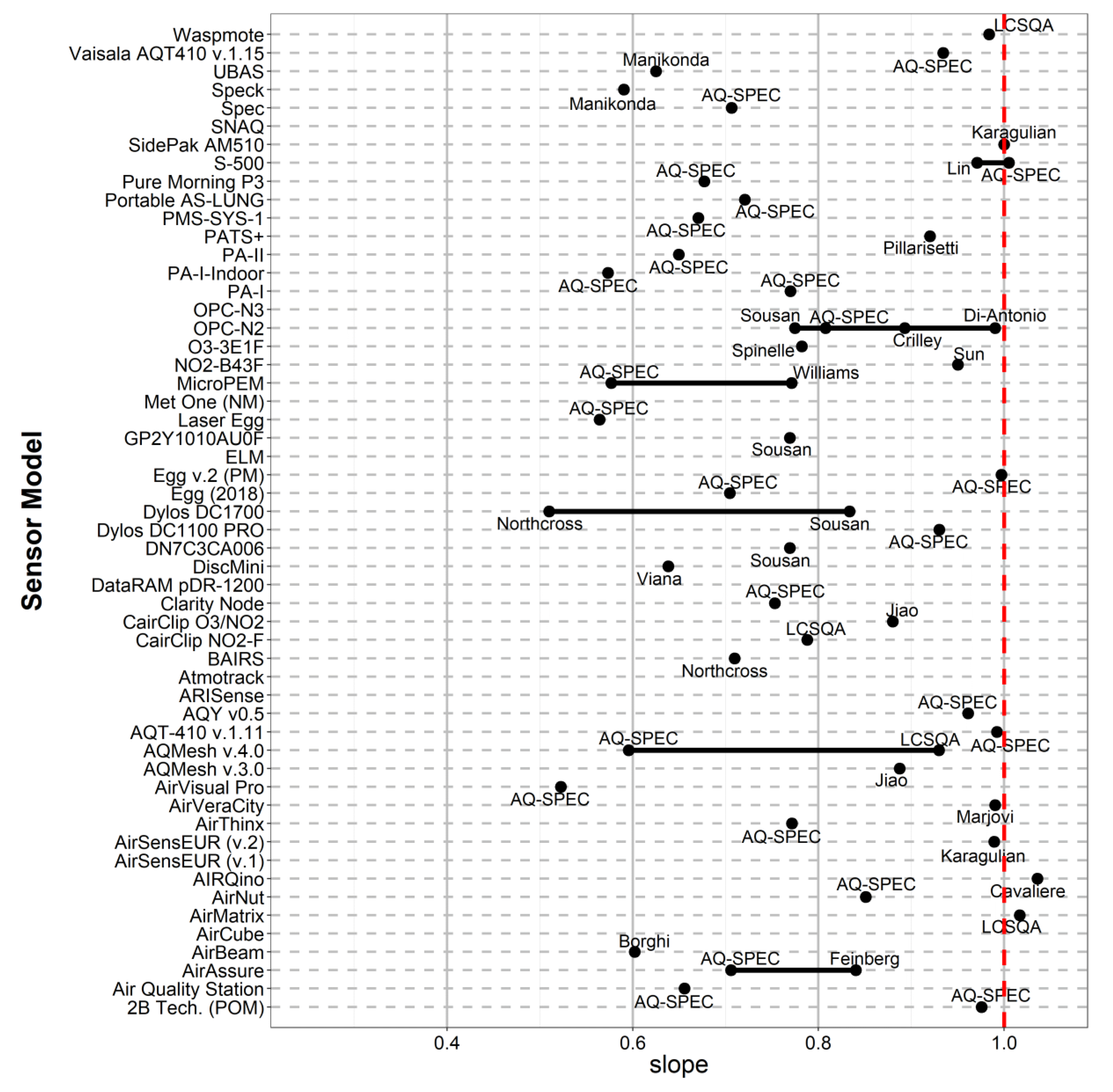
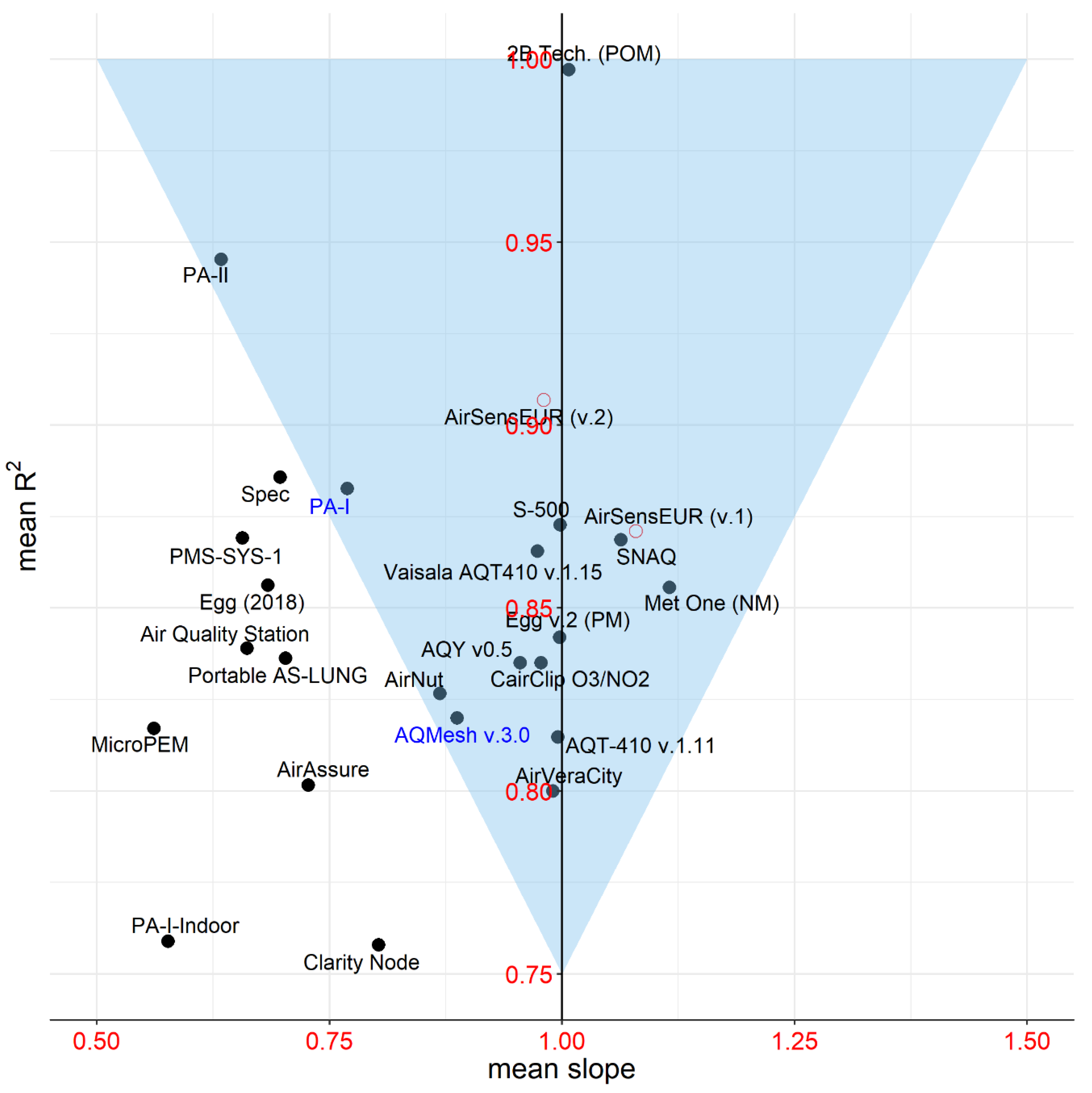
A list of SSys with R2 and slope close to 1.0 were drawn from the whole database of records of comparison tests of LCS data versus reference measurements, which indicates the best performance of SSys, as shown in Figure 8. In fact, in Figure 8 the blue background represents the best selection region for SSys. The best SSys would be the one that reaches the point with coordinates R² = 1 and slope = 1. Within the blue background region, the following SSys can be found: 2B Tech. (POM), PA-II, AirSensEUR (v.1), PA-I, S-500, AirSensEUR (v.1), SNAQ, Vaisala AQT410 v.15, MetOne (NM), the Egg (v.2), AQY v0.5, CairClip O3/NO2, AQMesh v3.0, AQT410 v.11, and AirVeraCity. Additionally, Figure 8 shows that there are more SSys underestimating reference measurements with slopes lower than 1 than SSys overestimating reference measurements.
Analyzing the SSys and their price, it was found that R² increases of 14% results in a 10-fold increase of the price of SSys—a limited improvement for a large price increase.
This review work clearly shows that there is a considerable number of field-work carried out with LCS. Therefore, field-calibrations were performed to correct outputs from LCS. However, as shown in recent work [27], during filed-calibrations it is not always possible to distinguish the single effect of each covariate that might affect the correct operation of the LCS. While this is only possible at controlled laboratory conditions, this could be overcome by co-locating clusters of sensors at reference sites to provide calibration outside of laboratory conditions.
Although this paper gives an exhaustive survey of the independent LCS evaluations, the concept of comparing LCS field tests from different studies can be difficult and may result in misleading conclusions. This is difficult because of the lack of uniformity in the metrics representing LCS data quality between studies and makes them difficult to compare. Comparing field tests of LCS may also be misleading, as in order to consider the highest number of studies it was necessary to rely on the coefficient of determination, R². However, R² is overly dependent on the range of reference measurements, on the duration of the test field, and on the season and location of the tests, meaning changes of R² are not completely dependent on LCS data quality or on calibration methods. This shortcoming makes the standardization of a protocol for evaluation of LCS at the international level a high priority, while inter-comparison exercises where LCS are gathered at the same test sites and at the same time are greatly needed.

Author Contributions

Conceptualization, F.K. and M.G.; methodology, F.K. and M.G.; software, F.K.; validation, F.K. and M.G; formal analysis, F.K. and M.G.; investigation, F.K. and M.G.; data curation, F.K., M.G., S.C., N.R., L.S., C.M., and B.H.; original draft preparation, F.K.; review and editing, F.K., M.G., A.K., L.S., M.B., and A.B.; visualization, F.K.; supervision, M.G.; project administration, A.B.; funding acquisition, A.B. and F.L.

Funding

This research was funded by the European Commission's Joint Research Centre and the Directorate General for Environment. The French inter-comparison exercise was funded by the French Ministry of Environment through the national reference laboratory for air quality monitoring (LCSQA).

Acknowledgments

We greatly acknowledge Julian Wilson for his help reviewing the whole work, as well as for checking English grammar.

Conflicts of Interest

The authors declare no conflict of interest. The funders had no role in the collection, analysis, or interpretation of data; in the writing of the manuscript, or in the decision to publish the results.

Appendix A

Table A1. Number of analyzed records and sensor models by averaging time.
Averaging Timen. Recordsn. OEMs and SSys
hourly61086
5 min25340
daily24842
1 min21433
Table A2. Model of OEMs by pollutant, type, openness, and price.
ModelPollutantTypeReferenceOpen/CloseLivingPrice
CO-B4COelectrochemicalWei [59]open sourceN50
CO 3E300COelectrochemicalGerboles [23]open sourceY100
DataRAM pDR-1200PM2.5nephelometerChakrabarti [70]black boxN-
DiscMiniPMOPCViana [77]open sourceY11,000
DN7C3CA006PM2.5nephelometerSousan [83]open sourceY10
DSM501APM2.5nephelometerWang [68], Alvarado [69]open sourceY15
FIS SP-61O3MOsSpinelle [26]open sourceY50
GP2Y1010AU0FPM2.5, PM10nephelometerOlivares [71], Manikonda [54], Sousan [83], Alvarado [69], Wang [68]open sourceY10
MiCS-2710NO2MOsSpinelle [20], Williams [30]open sourceN7
MICS-4514CO, NO2MOsSpinelle [20,24] open sourceY20
NO-3E100NOelectrochemicalSpinelle [24], Gerboles [23]open sourceY120
NO-B4NOelectrochemicalWei [59]open sourceY50
NO2-3E50NO2electrochemicalSpinelle [20], Gerboles [23]open sourceY100
NO2-A1NO2electrochemicalWilliams [30]black boxY50
NO2-B4NO2electrochemicalSpinelle [20,25] open sourceN50
NO2-B42FNO2electrochemicalWei [59]open sourceN50
NO2-B43FNO2electrochemicalSun [65]open sourceY50
O3-B4O3electrochemicalSpinelle [20,25], Wei [59]open source N50
O3-3E1FO3electrochemicalSpinelle [20,25], Gerboles [23]open sourceY500
OPC-N2PM1, PM2.5 OPCAQ-SPEC [19], Mukherjee [35], Sousan [83], Feinberg [36], Crilley [84], Badura [49], Crunaire [33]open source, black boxN362
OPC-N3PM1, PM2.5 OPCAQ-SPEC [19]open sourceY338
PMS1003PM2.5OPCKelly [75]black boxY20
PMS3003PM2.5OPCZheng [85], Kelly [75]open source, black boxY30
PMS5003PM2.5OPCLaquai [48]black boxY15
PMS7003PM2.5OPCBadura [49]black boxY20
PPD42NSPM2.5, PM3, PM2nephelometerWang [68], Holstius [51], Austin [73], Gao [74], Kelly [75]open sourceY15
SDS011PM2.5, OPCBudde [47], Laquai [48], Badura [49], Liu [52]open sourceY30
SM50O3MOsFeinberg [36]open sourceY500
TGS-5042COMOsSpinelle [24]open sourceY40
TZOA-PM Research SensorsPMnephelometerFeinberg [36]open sourceY90
ZH03APM2.5nephelometerBadura [49]black boxY20
Table A3. Models of Sensor Systems by pollutant, type, openness, and price.
ModelPollutantTypeReferenceOpen/CloseLivingPrice
2B Tech. (POM)O3UVAQ-SPEC [19]black boxY4500
Aeroqual-SM50O3MOsJiao [39]black boxY2000
AGT ATS-35 NO2NO2MOsWilliams [30]black boxN-d
Air Quality StationPM1, PM2.5OPCAQ-SPEC [19]black boxY2000
AirAssurePM2.5nephelometerAQ-SPEC [19], Feinberg [36], Manikonda [54]black boxY1500
AirBeamPM2.5OPC, nephelometerAQ-SPEC [19], Mukherjee [35], Feinberg [36], Borghi [37], Jiao [39], Crunaire [33]black boxY200
AirCubeNO2, O3, NOelectrochemicalMueller [43], Bigi [42]black boxY3538
AirMatrixPM1, PM2.5nephelometerCrunaire [33]black boxY60
AirNutPM2.5nephelometerAQ-SPEC [19]black boxY150
AIRQinoPM2.5 OPCCavaliere [76]open sourceY1000
AirSensEUR (v.1)NO, NO2, O3electrochemicalCrunaire [33]black boxY1600
AirSensEUR (v.2)CO, NO, NO2, O3electrochemicalKaragulian [22]open sourceY1600
AirSensorBoxNO2, CO, O3 electrochemical, MOs, nephelometerBorrego [53]black boxY280
AirThinxPM1, PM2.5 OPCAQ-SPEC [19]black boxY1000
AirVeraCityCO, NO2, O3electrochemical, MOsMarjovi [57]black boxY10000
AirVisual ProPM2.5 nephelometerAQ-SPEC [19]black boxY270
AQMesh v.3.0CO, NOelectrochemicalJiao [39]black boxN10000
AQMesh v.4.0NO2, CO, NO, O3electrochemicalCordero [63], AQ-SPEC [19], Castell [10], Borrego [53], Crunaire [33]black boxupdated10000
AQT410 v.1.11O3electrochemicalAQ-SPEC [19]black boxY3700
AQT-420NO2,O3, PM2.5electrochemical, OPCCrunaire [33]black boxY 3256
AQY v0.5PM2.5, NO2, O3OPC, electrochemical, MOsAQ-SPEC [19]black boxupdated3000
ARISenseNO2, CO, NO, O3electrochemicalCross [58]black boxY-
AtmotrackPM1, PM2.5nephelometerCrunaire [33]black boxY2500
BAIRSPM2.5–0.5OPCNorthcross [78]open sourceN475
CairPM2.5, PM10–2.5OPCAQ-SPEC [19]black boxY200
CairClip O3/NO2O3, NO2electrochemicalJiao [39], Spinelle [25], Williams [30], Duvall [64], Feinberg [36]black boxY600
CairClip NO2-FNO2electrochemicalSpinelle [20], Duvall [64], Crunaire [33]black boxY600
CairClip PM2.5PM2.5nephelometerWilliams [31]black boxY1500
CAMPM10, PM2.5, NO2, CO, NOOPC, electrochemicalBorrego [53]black boxY-
CanarITPMnephelometerWilliams [31]black boxN1500
Clarity NodePM2.5nephelometerAQ-SPEC [19]black boxY1300
Dylos DC1100PM2.5–0.5OPCJiao [39], Williams [31], Feinberg [36]black box, open sourceY300
Dylos DC1100 PROPM2.5–0, PM10–2.5, PM10OPCJiao [39], AQ-SPEC [19], Feinberg [36], Manikonda [54]black box, open sourceY300
Dylos DC1700PM2.5–0.5, PM10, PM10–2.5, PM3, PM2, PM2.5OPCManikonda [54], Sousan [83], Northcross [78], Holstius [51], Steinle [79], Han [80], Jovasevic [81], Dacunto [82]open sourceY475
e-PMPM10, PM2.5nephelometerCrunaire [33]black boxY2500
E-SamplerPM2.5OPCAQ-SPEC [19]black boxY5500
ECN_BoxPM10, PM2.5, NO2, O3nephelometer, electrochemicalBorrego [53]black boxY274
Eco PMPM1OPCWilliams [31]black boxN
ECOMSMARTNO2, O3, PM1, PM10, PM2.5electrochemical, OPCCrunaire [33]black boxY 4560
Egg (2018)PM1, PM2.5, PM10OPCAQ-SPEC [19]black boxY249
Egg v.1CO, NO2, O3MOsAQ-SPEC [19]black boxN200
Egg v.2CO, NO2, O3electrochemicalAQ-SPEC [19]black boxY240
Egg v.2 (PM)PM2.5, PM10nephelometerAQ-SPEC [19]black boxY280
ELMNO2, PM10, O3MOs, nephelometerAQ-SPEC [19], US-EPA [67]black boxN5200
EMMAPM2.5, CO, NO2, NOOPC, electrochemicalGillooly [60]black boxY-
ES-642PM2.5OPCCrunaire [33]black boxY2600
FoobotPM2.5OPCAQ-SPEC [19]black boxY200
Hanvon N1PM2.5nephelometerAQ-SPEC [19]black boxY200
Intel Berkeley BadgeNO2, O3electrochemical, MOsVaughn [32]open sourceN-
ISAGNO2, O3MOsBorrego [53]black boxN -
Laser EggPM2.5, PM10nephelometerAQ-SPEC [19]black boxY200
M-PODCO, NO2MOsPiedrahita [62]black boxN
MASCO, NO2, O3, PM2.5electrochemical, UV, nephelometerSun [40]black box, open sourceN, Y5500
Met One-831PM10OPCWilliams [31]black boxY2050
Met One (NM)PM2.5OPCAQ-SPEC [19]black boxY1900
MicroPEMPM2.5nephelometerAQ-SPEC [19], Williams [31]black boxY2000
NanoEnviNO2, O3, COelectrochemical, MOsBorrego [53]black boxY -
PA-IPM1, PM2.5, PM10OPCAQ-SPEC [19]black boxN150
PA-I-IndoorPM2.5, PM10OPCAQ-SPEC [19]black boxY180
PA-IIPM1, PM2.5, PM10OPCAQ-SPEC [19]black boxY200
PartectorPM1, PM2.5ElectricalAQ-SPEC [19]black boxY7000
PATS+PM2.5nephelometerPillarisetti [72]black boxY500
Platypus NO2NO2MOsWilliams [30]black boxY50
PMS-SYS-1PM2.5nephelometerJiao [39], AQ-SPEC [19], Williams [31], Feinberg [36]black boxY1000
Portable AS-LUNGPM1, PM2.5, PM10OPCAQ-SPEC [19]black boxY1000
Pure Morning P3PM2.5OPCAQ-SPEC [19]black boxY170
RAMPCO, NO2electrochemicalZimmerman [61]open sourceY -
S-500NO2, O3MOsLin [66], AQ-SPEC [19], Vaughn [32]black boxY500
SENS-ITO3, CO, NO2MOsAQ-SPEC [19]black boxN, Y2200
SidePak AM510PM2.5nephelometerKaragulian [28]open sourceY3000
Smart Citizen KitCOMOsAQ-SPEC [19]black boxY200
SNAQNO2, CO, NOelectrochemicalMead [44], Popoola [45]black boxY-
SpecCO, NO2, O3electrochemicalAQ-SPEC [19]black boxY500
SpeckPM2.5nephelometerFeinberg [36], US-EPA [67], Williams [31], AQ-SPEC [19], Manikonda [54], Zikova [55]black boxY150
UBASPM2.5nephelometerManikonda [54]black boxN100
uHooPM2.5, O3nephelometer, MOsAQ-SPEC [19]black boxY300
Urban AirQNO2electrochemicalMijling [41]open sourceN-
Vaisala AQT410 v.1.11CO, NO2electrochemicalAQ-SPEC [19]black boxY3700
Vaisala AQT410 v.1.15CO, NO2electrochemicalAQ-SPEC [19]black boxY3700
WaspmoteNO, NO2, PM1, PM10, PM2.5MOs, OPCCrunaire [33]black boxY1270
Watchtower 1NO2, PM1, PM10, PM2.5, O3electrochemical, OPCCrunaire [33]black boxY5000
Figure A1. Distribution of R2 for LCS hourly data against the reference for different pollutants. Dashed lines indicate the R² value of 0.7 and 1.0. Numbers in blue and black indicate the number of open source and black box records, respectively. Names of “living” and “non-living” sensors are indicated by black and red labels on the x-axis, respectively.
Atmosphere 10 00506 g0a1
Figure A2. Distribution of R2 for LCS minute data against the reference for different pollutants. Dashed lines indicate the R² value of 0.7 and 1.0. Numbers in blue and black indicate the number of open source and black box records, respectively. Names of “living” and “non-living” sensors are indicated in black and red labels of the x-axis color, respectively.
Atmosphere 10 00506 g0a2
Figure A3. Distribution of R2 from the comparison of SSys minute data against reference measurements. Numbers in blue and black indicate the number of open source and black box records, respectively. Names of “living” and “non-living” sensors are indicated by black and red labels on the x-axis, respectively.
Atmosphere 10 00506 g0a3
Figure A4. Distribution of R2 from the comparison of SSys hourly data against reference measurements. Numbers in blue and black indicate the number of open source and black box records, respectively. Names of “living” and “non-living” sensors are indicated by black and red labels on the x-axis, respectively.
Atmosphere 10 00506 g0a4
Figure A5. Distribution of R2 from the comparison of all OEMs against reference systems. Records were averaged over a time-scale of 1 h. Numbers in blue and black indicate the number of open source and black box records, respectively. Names of “living” and “non-living” sensors are indicated by black and red labels on the x-axis, respectively.
Atmosphere 10 00506 g0a5
Figure A6. Distribution of R2 from the comparison of all OEMs against reference systems. Records were averaged over a time-scale of daily data. Numbers in blue and black indicate the number of open source and black box records, respectively. Names of “living” and “non-living” sensors are indicated by black and red labels on the x-axis, respectively.
Atmosphere 10 00506 g0a6
Figure A7. Distribution of R2 from the comparison of all sensor systems against reference systems. Records were averaged over a time-scale of daily data. Numbers in blue and black indicate the number of open source and black box records, respectively. Names of “living” and “non-living” sensors are indicated by black and red labels on the x-axis, respectively.
Atmosphere 10 00506 g0a7
Figure A8. Distribution of slopes from the comparison of SSys against the reference. Only records with R2 > 0.7 and 0.5 < slope < 1.5 are shown. Records were averaged over a time-scale of 1 h. Numbers in blue and black indicate the number of open source and black box records, respectively. Names of “living” and “non-living” sensors are indicated by black and red labels on the x-axis, respectively.
Atmosphere 10 00506 g0a8
Figure A9. Distribution of slopes from the comparison of OEMs against the reference. Only hourly records with R2 > 0.7 and 0.5 < slope < 1.5 are shown. Numbers in blue and black indicate the number of open source and black box records, respectively. Names of “living” and “non-living” sensors are indicated by black and red labels on the x-axis, respectively.
Atmosphere 10 00506 g0a9
Figure A10. Distribution of slopes from the comparison of SSys against the reference. Only records with R2 > 0.7 and 0.5 < slope < 1.5 are shown. Records were averaged over a time-scale of daily data. Numbers in blue and black indicate the number of open source and black box records, respectively. Names of “living” and “non-living” sensors are indicated by black and red labels on the x-axis, respectively.
Atmosphere 10 00506 g0a10
Figure A11. Distribution of slopes from the comparison of OEMs against the reference. Only records with R2 > 0.7 and 0.5 < slope < 1.5 are shown. Records were averaged over a time-scale of daily data. Numbers in blue and black indicate the number of open source and black box records, respectively. Names of “living” and “non-living” sensors are indicated by black and red labels on the x-axis, respectively.
Atmosphere 10 00506 g0a11
Figure A12. Mean slope obtained from the comparison of LCS against reference measurements.
Atmosphere 10 00506 g0a12
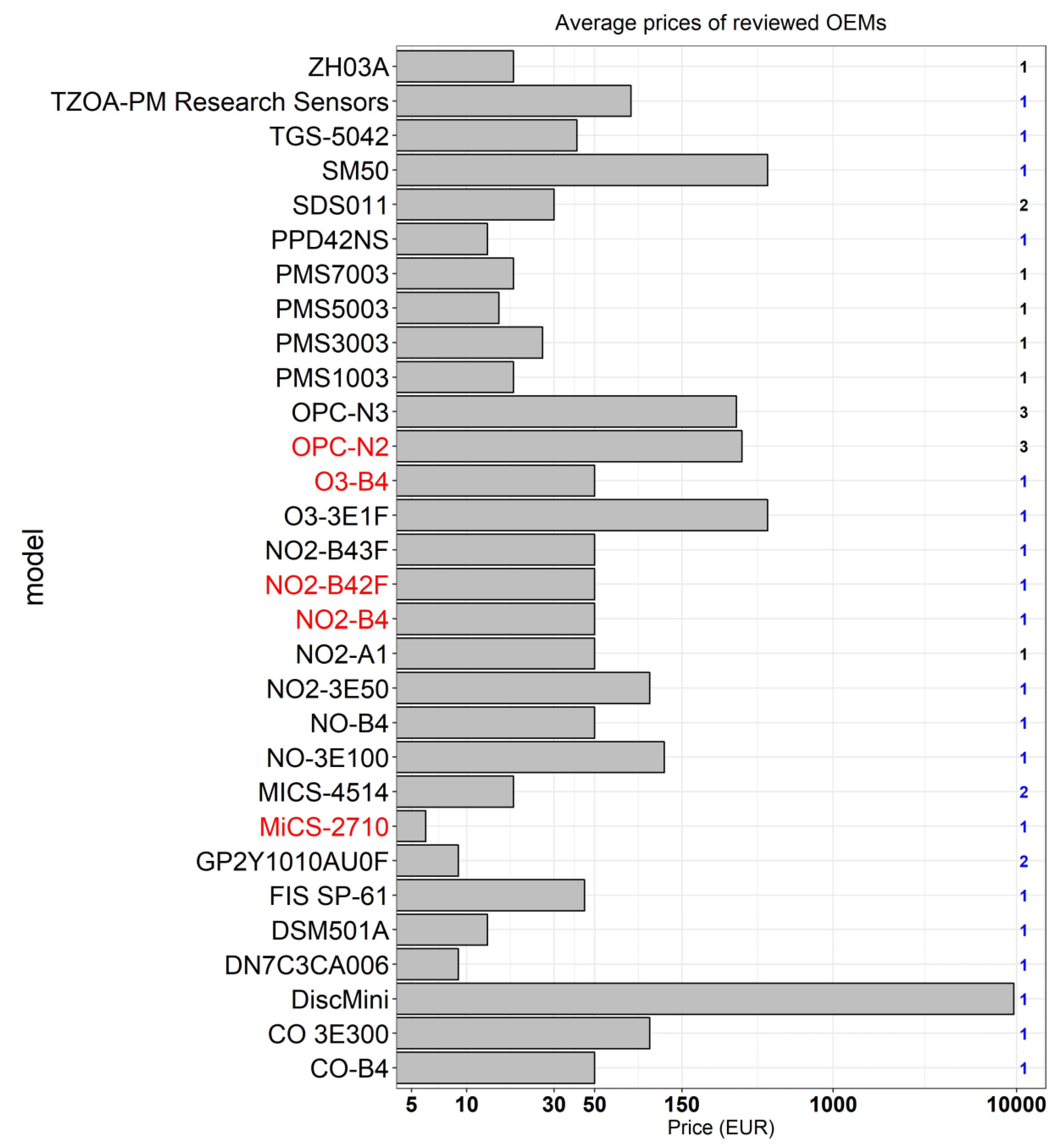
Figure A13. Prices of OEMs grouped by model. Numbers at right indicates the number of pollutants measured by each OEMs, with open source in blue and black box in black. The x-axis uses a logarithmic scale. Names of “living” and “non-living” OEMs are indicated by black and red for the labels on the y-axis, respectively.
Atmosphere 10 00506 g0a13
Table A4. Shortlist of SSys showing good agreement with reference systems (R2 > 0.85; 0.8 < slope < 1.2) for daily data.
ModelPollutantMeanMean SlopeMean Absolute InterceptOpen/CloseLivingCommercialPrice (EUR)
PA-IPM10.990.90.47black boxNcommercial132
PA-IIPM10.990.81.8black boxYcommercial176
Egg (2018)PM10.880.80.33black boxYcommercial219
Egg v.2 (PM)PM2.50.9413.3black boxYcommercial246
AirThinxPM10.890.81.3black boxYcommercial880
Portable AS-LUNGPM10.930.91.5black boxYnon-commercial880
AIRQinoPM2.5, PM100.9111.1open sourceYnon-commercial1000
Air Quality StationPM10.940.91.1black boxYnon-commercial1760
AQY v0.5PM2.50.910.94.0black boxupdatedcommercial2640
Vaisala AQT410 v.1.15CO0.860.90.25black boxYcommercial3256

References

  1. Kumar, P.; Morawska, L.; Martani, C.; Biskos, G.; Neophytou, M.; Di Sabatino, S.; Bell, M.; Norford, L.; Britter, R. The rise of low-cost sensing for managing air pollution in cities. Environ. Int. 2015, 75, 199–205. [Google Scholar] [CrossRef] [PubMed] [Green Version]
  2. 2008/50/EC: Directive of the European Parliament and of the Council of 21 May 2008 on ambient air quality and cleaner air for Europe. Available online: http://eurlex.europa.eu/Result.do?RechType=RECH_celex&lang=en&code=32008L0050 (accessed on 22 August 2019).
  3. CEN. Ambient Air—Standard Gravimetric Measurement Method for the Determination of the PM10 or PM2,5 Mass Concentration of Suspended Particulate Matter (EN 12341:2014); European Committee for Standardization: Brussels, Belgium, 2014. [Google Scholar]
  4. CEN Ambient Air. Standard Method for the Measurement of the Concentration of Carbon Monoxide by Non-Dispersive Infrared Spectroscopy, (EN 14626:2012); European Committee for Standardization: Brussels, Belgium, 2012. [Google Scholar]
  5. CEN Ambient Air. Standard Method for the Measurement of the Concentration of Nitrogen Dioxide and Nitrogen Monoxide by Chemiluminescence (EN 14211:2012); European Committee for Standardization: Brussels, Belgium, 2012. [Google Scholar]
  6. CEN Ambient Air. Standard Method for the Measurement of the Concentration of Ozone by Ultraviolet Photometry (EN 14625:2012); European Committee for Standardization: Brussels, Belgium, 2012. [Google Scholar]
  7. CEN Ambient Air. Standard Method for the Measurement of the Concentration of Sulphur Dioxide by Ultraviolet Fluorescence, (EN 14212:2012); European Committee for Standardization: Brussels, Belgium, 2012. [Google Scholar]
  8. Lewis, A.C.; von Schneidemesser, E.; Peltier, R. Low-cost sensors for the measurement of atmospheric composition: overview of topic and future applications (World Meteorological Organization). Available online: https://www.ccacoalition.org/en/resources/low-cost-sensors-measurement-atmospheric-composition-overview-topic-and-future (accessed on 21 August 2019).
  9. Aleixandre, M.; Gerboles, M. Review of small commercial sensors for indicative monitoring of ambient gas. Chem. Eng. Trans. 2012, 30, 169–174. [Google Scholar]
  10. Castell, N.; Dauge, F.R.; Schneider, P.; Vogt, M.; Lerner, U.; Fishbain, B.; Broday, D.; Bartonova, A. Can commercial low-cost sensor platforms contribute to air quality monitoring and exposure estimates? Environ. Int. 2017, 99, 293–302. [Google Scholar] [CrossRef] [PubMed]
  11. iScape. Summary of Air Quality sensors and recommendations for application. Available online: https://www.iscapeproject.eu/wp-content/uploads/2017/09/iSCAPE_D1.5_Summary-of-air-quality-sensors-and-recommendations-for-application.pdf (accessed on 21 August 2019).
  12. Snyder, E.G.; Watkins, T.H.; Solomon, P.A.; Thoma, E.D.; Williams, R.W.; Hagler, G.S.W.; Shelow, D.; Hindin, D.A.; Kilaru, V.J.; Preuss, P.W. The changing paradigm of air pollution monitoring. Environ. Sci. Technol. 2013, 47, 11369–11377. [Google Scholar] [CrossRef] [PubMed]
  13. White, R.M.; Paprotny, I.; Doering, F.; Cascio, W.E.; Solomon, P.A.; Gundel, L.A. Sensors and “apps” for community-based: Atmospheric monitoring. EM Air Waste Manag. Assoc. Mag. Environ. Manag. 2012, 5, 36–40. [Google Scholar]
  14. Williams, R.; Kilaru, V.; Snyder, E.; Kaufman, A.; Dye, T.; Rutter, A.; Russell, A.; Hafner, H. Air Sensor Guidebook; United States Environmental Protection Agency (US-EPA): Washington, DC, USA, 2014. [Google Scholar]
  15. Zhou, X.; Lee, S.; Xu, Z.; Yoon, J. Recent Progress on the Development of Chemosensors for Gases. Chem. Rev. 2015, 115, 7944–8000. [Google Scholar] [CrossRef] [PubMed]
  16. Spinelle, L.; Aleixandre, M.; Gerboles, M. Protocol of Evaluation and Calibration of Low-Cost Gas Sensors for the Monitoring of Air Pollution; Publications Office of the European Union: Luxembourg, 2013. [Google Scholar]
  17. Redon, N.; Delcourt, F.; Crunaire, S.; Locoge, N. Protocole de détermination des caractéristiques de performance métrologique des micro-capteurs-étude comparative des performances en laboratoire de micro-capteurs de NO2 | LCSQA. Available online: https://www.lcsqa.org/fr/rapport/2016/mines-douai/protocole-determination-caracteristiques-performance-metrologique-micro-cap (accessed on 22 August 2019).
  18. Williams, R.; Duvall, R.; Kilaru, V.; Hagler, G.; Hassinger, L.; Benedict, K.; Rice, J.; Kaufman, A.; Judge, R.; Pierce, G.; et al. Deliberating performance targets workshop: Potential paths for emerging PM2.5 and O3 air sensor progress. Atmos. Environ. X 2019, 2, 100031. [Google Scholar] [CrossRef]
  19. AQ-SPEC; South Coast Air Quality Management District; South Coast Air Quality Management District Air Quality Sensor Performance Evaluation Reports. Available online: http://www.aqmd.gov/aq-spec/evaluations#&MainContent_C001_Col00=2 (accessed on 29 December 2015).
  20. Spinelle, L.; Gerboles, M.; Villani, M.G.; Aleixandre, M.; Bonavitacola, F. Field calibration of a cluster of low-cost available sensors for air quality monitoring. Part A: Ozone and nitrogen dioxide. Sens. Actuators B Chem. 2015, 215, 249–257. [Google Scholar] [CrossRef]
  21. Lewis, A.; Edwards, P. Validate personal air-pollution sensors. Nat. News 2016, 535, 29. [Google Scholar] [CrossRef]
  22. Karagulian, F.; Borowiak, A.; Barbiere, M.; Kotsev, A.; van der Broecke, J.; Vonk, J.; Signorini, M.; Gerboles, M. Calibration of AirSensEUR Units during a Field Study in the Netherlands; European Commission-Joint Research Centre: Ispra, Italy, 2019; in press. [Google Scholar]
  23. Gerboles, M.; Spinelle, L.; Signorini, M. AirSensEUR: An Open Data/Software/Hardware Multi-Sensor Platform for Air Quality Monitoring. Part A: Sensor Shield; Publications Office of the European Union: Luxembourg, 2015. [Google Scholar]
  24. Spinelle, L.; Gerboles, M.; Villani, M.G.; Aleixandre, M.; Bonavitacola, F. Field calibration of a cluster of low-cost commercially available sensors for air quality monitoring. Part B: NO, CO and CO2. Sens. Actuators B Chem. 2017, 238, 706–715. [Google Scholar] [CrossRef]
  25. Spinelle, L.; Gerboles, M.; Aleixandre, M. Performance Evaluation of Amperometric Sensors for the Monitoring of O 3 and NO 2 in Ambient Air at ppb Level. Procedia Eng. 2015, 120, 480–483. [Google Scholar] [CrossRef]
  26. Spinelle, L.; Gerboles, M.; Aleixandre, M.; Bonavitacola, F. Evaluation of metal oxides sensors for the monitoring of O3 in ambient air at ppb level. Chem. Eng. Trans. 2016, 319–324. [Google Scholar]
  27. Spinelle, L.; Gerboles, M.; Kotsev, A.; Signorini, M. Evaluation of Low-Cost Sensors for Air Pollution Monitoring: Effect of Gaseous Interfering Compounds and Meteorological Conditions; Publications Office of the European Union: Luxembourg, 2017. [Google Scholar]
  28. Karagulian, F.; Belis, C.A.; Lagler, F.; Barbiere, M.; Gerboles, M. Evaluation of a portable nephelometer against the Tapered Element Oscillating Microbalance method for monitoring PM2.5. J. Env. Monit. 2012, 14, 2145–2153. [Google Scholar] [CrossRef] [PubMed]
  29. US-EPA. Air Sensor Toolbox; Evaluation of Emerging Air Pollution Sensor Performance. US-EPA. Available online: https://www.epa.gov/air-sensor-toolbox/evaluation-emerging-air-pollution-sensor-performance (accessed on 21 August 2018).
  30. Williams, R.; Long, R.; Beaver, M.; Kaufman, A.; Zeiger, F.; Heimbinder, M.; Acharya, B.R.; Grinwald, B.A.; Kupcho, K.A.; Tobinson, S.E. Sensor Evaluation Report; U.S. Environmental Protection Agency: Washington, DC, USA, 2014. [Google Scholar]
  31. Williams, R.; Kaufman, A.; Hanley, T.; Rice, J.; Garvey, S. Evaluation of Field-deployed Low Cost PM Sensors; U.S. Environmental Protection Agency: Washington, DC, USA, 2014. [Google Scholar]
  32. Vaughn, D.L.; Dye, T.S.; Roberts, P.T.; Ray, A.E.; DeWinter, J.L. Characterization of low-Cost NO2 Sensors; U.S. Environmental Protection Agency: Washington, DC, USA, 2010. [Google Scholar]
  33. Crunaire, S.; Redon, N.; Spinelle, L. 1ER Essai national d’Aptitude des Microcapteurs EAμC) pour la Surveillance de la Qualité de l’Air: Synthèse des Résultas; LCSQA: Paris, France, 2018; p. 38. [Google Scholar]
  34. Fishbain, B.; Lerner, U.; Castell, N.; Cole-Hunter, T.; Popoola, O.; Broday, D.M.; Iñiguez, T.M.; Nieuwenhuijsen, M.; Jovasevic-Stojanovic, M.; Topalovic, D.; et al. An evaluation tool kit of air quality micro-sensing units. Sci. Total Environ. 2017, 575, 639–648. [Google Scholar] [CrossRef] [PubMed]
  35. Mukherjee, A.; Stanton, L.G.; Graham, A.R.; Roberts, P.T. Assessing the Utility of Low-Cost Particulate Matter Sensors over a 12-Week Period in the Cuyama Valley of California. Sensors 2017, 17, 1805. [Google Scholar] [CrossRef] [PubMed]
  36. Feinberg, S.; Williams, R.; Hagler, G.S.W.; Rickard, J.; Brown, R.; Garver, D.; Harshfield, G.; Stauffer, P.; Mattson, E.; Judge, R.; et al. Long-term evaluation of air sensor technology under ambient conditions in Denver, Colorado. Atmos. Meas. Tech. 2018, 11, 4605–4615. [Google Scholar] [CrossRef] [Green Version]
  37. Borghi, F.; Spinazzè, A.; Campagnolo, D.; Rovelli, S.; Cattaneo, A.; Cavallo, D.M. Precision and Accuracy of a Direct-Reading Miniaturized Monitor in PM2.5 Exposure Assessment. Sensors 2018, 18, 3089. [Google Scholar] [CrossRef]
  38. Zikova, N.; Masiol, M.; Chalupa, D.C.; Rich, D.Q.; Ferro, A.R.; Hopke, P.K. Estimating Hourly Concentrations of PM2.5 across a Metropolitan Area Using Low-Cost Particle Monitors. Sensor (Basel) 2017, 17, 1992. [Google Scholar] [CrossRef]
  39. Jiao, W.; Hagler, G.; Williams, R.; Sharpe, R.; Brown, R.; Garver, D.; Judge, R.; Caudill, M.; Rickard, J.; Davis, M.; et al. Community Air Sensor Network (CAIRSENSE) project: evaluation of low-cost sensor performance in a suburban environment in the southeastern United States. Atmos. Meas. Tech. 2016, 9, 5281–5292. [Google Scholar] [CrossRef] [Green Version]
  40. Sun, L.; Wong, K.C.; Wei, P.; Ye, S.; Huang, H.; Yang, F.; Westerdahl, D.; Louie, P.K.K.; Luk, C.W.Y.; Ning, Z. Development and Application of a Next Generation Air Sensor Network for the Hong Kong Marathon 2015 Air Quality Monitoring. Sensor (Basel) 2017, 17, 1922. [Google Scholar] [CrossRef]
  41. Mijling, B.; Jiang, Q.; de Jonge, D.; Bocconi, S. Practical field calibration of electrochemical NO2 sensors for urban air quality applications. Atmos. Meas. Tech. Discuss. 2017, 2017, 1–25. [Google Scholar] [CrossRef]
  42. Bigi, A.; Mueller, M.; Grange, S.K.; Ghermandi, G.; Hueglin, C. Performance of NO, NO2 low cost sensors and three calibration approaches within a real world application. Atmos. Meas. Tech. 2018, 11, 3717–3735. [Google Scholar] [CrossRef]
  43. Mueller, M.; Meyer, J.; Hueglin, C. Design of an ozone and nitrogen dioxide sensor unit and its long-term operation within a sensor network in the city of Zurich. Atmos. Meas. Tech. 2017, 10, 3783–3799. [Google Scholar] [CrossRef] [Green Version]
  44. Mead, M.I.; Popoola, O.A.M.; Stewart, G.B.; Landshoff, P.; Calleja, M.; Hayes, M.; Baldovi, J.J.; McLeod, M.W.; Hodgson, T.F.; Dicks, J.; et al. The use of electrochemical sensors for monitoring urban air quality in low-cost, high-density networks. Atmos. Environ. 2013, 70, 186–203. [Google Scholar] [CrossRef] [Green Version]
  45. Popoola, O.A.M.; Stewart, G.B.; Mead, M.I.; Jones, R.L. Development of a baseline-temperature correction methodology for electrochemical sensors and its implications for long-term stability. Atmos. Environ. 2016, 147, 330–343. [Google Scholar] [CrossRef] [Green Version]
  46. Mooney, D.; Willis, P.; Stevenson, K. A Guide for Local Authorities Purchasing Air Quality Monitoring Equipment. Available online: https://uk-air.defra.gov.uk/library/reports?report_id=386 (accessed on 21 August 2019).
  47. Budde, M.; Müller, T.; Laquai, B.; Streibl, N.; Schwarz, A.; Schindler, G.; Riedel, T.; Beigl, M.; Dittler, A. Suitability of the Low-Cost SDS011 Particle Sensor for Urban PM-Monitoring. In Proceedings of the 3rd International Conference on Atmospheric Dust, Bari, Italy, 29–31 May 2018. [Google Scholar]
  48. Laquai, B. Particle Distribution Dependent Inaccuracy of the Plantower PMS5003 low-cost PM-sensor. Available online: https://www.researchgate.net/publication/320555036 (accessed on 21 August 2019).
  49. Budde, M.; Müller, T.; Laquai, B.; Streibl, N.; Schwarz, A.; Schindler, G.; Riedel, T.; Beigl, M.; Dittler, A. Optical particulate matter sensors in PM2.5 measurements in atmospheric air. E3S Web Conf. 2018, 44, 00006. [Google Scholar]
  50. The World Air Quality Index. Sensing the Air Quality: Research on Air Quality Sensors. Available online: http://aqicn.org/sensor/ (accessed on 21 August 2019).
  51. Holstius, D.M.; Pillarisetti, A.; Smith, K.R.; Seto, E. Field calibrations of a low-cost aerosol sensor at a regulatory monitoring site in California. Atmos. Meas. Tech. 2014, 7, 1121–1131. [Google Scholar] [CrossRef] [Green Version]
  52. Liu, H.-Y.; Schneider, P.; Haugen, R.; Vogt, M. Performance Assessment of a Low-Cost PM2.5 Sensor for a near Four-Month Period in Oslo, Norway. Atmosphere 2019, 10, 41. [Google Scholar] [CrossRef]
  53. Borrego, C.; Costa, A.M.; Ginja, J.; Amorim, M.; Coutinho, M.; Karatzas, K.; Sioumis, Th.; Katsifarakis, N.; Konstantinidis, K.; De Vito, S.; et al. Assessment of air quality microsensors versus reference methods: The EuNetAir joint exercise. Atmos. Environ. 2016, 147, 246–263. [Google Scholar] [CrossRef] [Green Version]
  54. Manikonda, A.; Zíková, N.; Hopke, P.K.; Ferro, A.R. Laboratory assessment of low-cost PM monitors. J. Aerosol Sci. 2016, 102, 29–40. [Google Scholar] [CrossRef]
  55. Zikova, N.; Hopke, P.K.; Ferro, A.R. Evaluation of new low-cost particle monitors for PM2.5 concentrations measurements. J. Aerosol Sci. 2017, 105, 24–34. [Google Scholar] [CrossRef]
  56. Sousan, S.; Koehler, K.; Hallett, L.; Peters, T.M. Evaluation of the Alphasense optical particle counter (OPC-N2) and the Grimm portable aerosol spectrometer (PAS-1.108). Aerosol Sci. Technol. 2016, 50, 1352–1365. [Google Scholar] [CrossRef] [PubMed]
  57. Marjovi, A.; Arfire, A.; Martinoli, A. Extending Urban Air Quality Maps Beyond the Coverage of a Mobile Sensor Network: Data Sources, Methods, and Performance Evaluation. In Proceedings of the 2017 International Conference on Embedded Wireless Systems and Networks, Uppsala, Sweden, 20–22 February 2017; pp. 12–23. [Google Scholar]
  58. Cross, E.S.; Williams, L.R.; Lewis, D.K.; Magoon, G.R.; Onasch, T.B.; Kaminsky, M.L.; Worsnop, D.R.; Jayne, J.T. Use of electrochemical sensors for measurement of air pollution: correcting interference response and validating measurements. Atmos. Meas. Tech. 2017, 10, 3575–3588. [Google Scholar] [CrossRef] [Green Version]
  59. Wei, P.; Ning, Z.; Ye, S.; Sun, L.; Yang, F.; Wong, K.; Westerdahl, D.; Louie, P. Impact Analysis of Temperature and Humidity Conditions on Electrochemical Sensor Response in Ambient Air Quality Monitoring. Sensors 2018, 18, 59. [Google Scholar] [CrossRef] [PubMed]
  60. Gillooly, S.E.; Zhou, Y.; Vallarino, J.; Chu, M.T.; Michanowicz, D.R.; Levy, J.I.; Adamkiewicz, G. Development of an in-home, real-time air pollutant sensor platform and implications for community use. Environ. Pollut. 2019, 244, 440–450. [Google Scholar] [CrossRef]
  61. Zimmerman, N.; Presto, A.A.; Kumar, S.P.N.; Gu, J.; Hauryliuk, A.; Robinson, E.S.; Robinson, A.L.; Subramanian, R. A machine learning calibration model using random forests to improve sensor performance for lower-cost air quality monitoring. Atmos. Meas. Tech. 2018, 11, 291–313. [Google Scholar] [CrossRef] [Green Version]
  62. Piedrahita, R.; Xiang, Y.; Masson, N.; Ortega, J.; Collier, A.; Jiang, Y.; Li, K.; Dick, R.P.; Lv, Q.; Hannigan, M.; et al. The next generation of low-cost personal air quality sensors for quantitative exposure monitoring. Atmos. Meas. Tech 2014, 7, 3325–3336. [Google Scholar] [CrossRef] [Green Version]
  63. Cordero, J.M.; Borge, R.; Narros, A. Using statistical methods to carry out in field calibrations of low cost air quality sensors. Sens. Actuators B Chem. 2018, 267, 245–254. [Google Scholar] [CrossRef]
  64. Duvall, R.M.; Long, R.W.; Beaver, M.R.; Kronmiller, K.G.; Wheeler, M.L.; Szykman, J.J. Performance Evaluation and Community Application of Low-Cost Sensors for Ozone and Nitrogen Dioxide. Sensors 2016, 16, 1698. [Google Scholar] [CrossRef]
  65. Sun, L.; Westerdahl, D.; Ning, Z. Development and Evaluation of A Novel and Cost-Effective Approach for Low-Cost NO2 Sensor Drift Correction. Sensors 2017, 17, 1916. [Google Scholar] [CrossRef]
  66. Lin, C.; Gillespie, J.; Schuder, M.D.; Duberstein, W.; Beverland, I.J.; Heal, M.R. Evaluation and calibration of Aeroqual series 500 portable gas sensors for accurate measurement of ambient ozone and nitrogen dioxide. Atmos. Environ. 2015, 100, 111–116. [Google Scholar] [CrossRef]
  67. US-EPA. Evaluation of Elm and Speck Sensors. Available online: https://cfpub.epa.gov/si/si_public_record_report.cfm?Lab=NERL&dirEntryId=310285 (accessed on 21 August 2019).
  68. Wang, Y.; Li, J.; Jing, H.; Zhang, Q.; Jiang, J.; Biswas, P. Laboratory Evaluation and Calibration of Three Low-Cost Particle Sensors for Particulate Matter Measurement. Aerosol Sci. Technol. 2015, 49, 1063–1077. [Google Scholar] [CrossRef]
  69. Alvarado, M.; Gonzalez, F.; Fletcher, A.; Doshi, A.; Alvarado, M.; Gonzalez, F.; Fletcher, A.; Doshi, A. Towards the Development of a Low Cost Airborne Sensing System to Monitor Dust Particles after Blasting at Open-Pit Mine Sites. Sensors 2015, 15, 19667–19687. [Google Scholar] [CrossRef] [PubMed] [Green Version]
  70. Chakrabarti, B.; Fine, P.M.; Delfino, R.; Sioutas, C. Performance evaluation of the active-flow personal DataRAM PM2.5 mass monitor (Thermo Anderson pDR-1200) designed for continuous personal exposure measurements. Atmos. Environ. 2004, 38, 3329–3340. [Google Scholar] [CrossRef]
  71. Olivares, G.; Edwards, S. The Outdoor Dust Information Node (ODIN) – development and performance assessment of a low cost ambient dust sensor. Atmos. Meas. Tech. Discuss. 2015, 8, 7511–7533. [Google Scholar] [CrossRef]
  72. Pillarisetti, A.; Allen, T.; Ruiz-Mercado, I.; Edwards, R.; Chowdhury, Z.; Garland, C.; Hill, L.D.; Johnson, M.; Litton, C.D.; Lam, N.L.; et al. Small, Smart, Fast, and Cheap: Microchip-Based Sensors to Estimate Air Pollution Exposures in Rural Households. Sensor. (Basel) 2017, 17, 1879. [Google Scholar] [CrossRef] [PubMed]
  73. Austin, E.; Novosselov, I.; Seto, E.; Yost, M.G. Laboratory Evaluation of the Shinyei PPD42NS Low-Cost Particulate Matter Sensor. Plos ONE 2015, 10, e0137789. [Google Scholar]
  74. Gao, M.; Cao, J.; Seto, E. A distributed network of low-cost continuous reading sensors to measure spatiotemporal variations of PM2.5 in Xi’an, China. Environ. Pollut. 2015, 199, 56–65. [Google Scholar] [CrossRef] [PubMed]
  75. Kelly, K.E.; Whitaker, J.; Petty, A.; Widmer, C.; Dybwad, A.; Sleeth, D.; Martin, R.; Butterfield, A. Ambient and laboratory evaluation of a low-cost particulate matter sensor. Environ. Pollut. 2017, 221, 491–500. [Google Scholar] [CrossRef]
  76. Cavaliere, A.; Carotenuto, F.; Di Gennaro, F.; Gioli, B.; Gualtieri, G.; Martelli, F.; Matese, A.; Toscano, P.; Vagnoli, C.; Zaldei, A. Development of Low-Cost Air Quality Stations for Next Generation Monitoring Networks: Calibration and Validation of PM2.5 and PM10 Sensors. Sensors 2018, 18, 2843. [Google Scholar] [CrossRef]
  77. Viana, M.; Rivas, I.; Reche, C.; Fonseca, A.S.; Pérez, N.; Querol, X.; Alastuey, A.; Álvarez-Pedrerol, M.; Sunyer, J. Field comparison of portable and stationary instruments for outdoor urban air exposure assessments. Atmos. Environ. 2015, 123 Pt A, 220–228. [Google Scholar] [CrossRef]
  78. Northcross, A.L.; Edwards, R.J.; Johnson, M.A.; Wang, Z.-M.; Zhu, K.; Allen, T.; Smith, K.R. A low-cost particle counter as a realtime fine-particle mass monitor. Env. Sci. Process. Impacts 2013, 15, 433–439. [Google Scholar] [CrossRef] [PubMed]
  79. Steinle, S.; Reis, S.; Sabel, C.E.; Semple, S.; Twigg, M.M.; Braban, C.F.; Leeson, S.R.; Heal, M.R.; Harrison, D.; Lin, C.; et al. Personal exposure monitoring of PM 2.5 in indoor and outdoor microenvironments. Sci. Total Environ. 2015, 508, 383–394. [Google Scholar] [CrossRef] [PubMed] [Green Version]
  80. Han, I.; Symanski, E.; Stock, T.H. Feasibility of using low-cost portable particle monitors for measurement of fine and coarse particulate matter in urban ambient air. J. Air Waste Manag. Assoc. 2017, 67, 330–340. [Google Scholar] [CrossRef] [PubMed]
  81. Jovašević-Stojanović, M.; Bartonova, A.; Topalović, D.; Lazović, I.; Pokrić, B.; Ristovski, Z. On the use of small and cheaper sensors and devices for indicative citizen-based monitoring of respirable particulate matter. Environ. Pollut. 2015, 206, 696–704. [Google Scholar] [CrossRef] [PubMed]
  82. Dacunto, P.J.; Klepeis, N.E.; Cheng, K.-C.; Acevedo-Bolton, V.; Jiang, R.-T.; Repace, J.L.; Ott, W.R.; Hildemann, L.M. Determining PM2.5 calibration curves for a low-cost particle monitor: common indoor residential aerosols. Environ. Sci. Process. Impacts 2015, 17, 1959–1966. [Google Scholar] [CrossRef] [PubMed]
  83. Sousan, S.; Koehler, K.; Thomas, G.; Park, J.H.; Hillman, M.; Halterman, A.; Peters, T.M. Inter-comparison of low-cost sensors for measuring the mass concentration of occupational aerosols. Aerosol Sci. Technol. 2016, 50, 462–473. [Google Scholar] [CrossRef] [Green Version]
  84. Crilley, L.R.; Shaw, M.; Pound, R.; Kramer, L.J.; Price, R.; Young, S.; Lewis, A.C.; Pope, F.D. Evaluation of a low-cost optical particle counter (Alphasense OPC-N2) for ambient air monitoring. Atmos. Meas. Tech. 2018, 11, 709–720. [Google Scholar] [CrossRef] [Green Version]
  85. Zheng, T.; Bergin, M.H.; Johnson, K.K.; Tripathi, S.N.; Shirodkar, S.; Landis, M.S.; Sutaria, R.; Carlson, D.E. Field evaluation of low-cost particulate matter sensors in high and low concentration environments. Atmos. Meas. Tech. Discuss. 2018, 11, 4823–4846. [Google Scholar] [CrossRef]
  86. Esposito, E.; Salvato, M.; Vito, S.D.; Fattoruso, G.; Castell, N.; Karatzas, K.; Francia, G.D. Assessing the Relocation Robustness of on Field Calibrations for Air Quality Monitoring Devices. In Proceedings of the Sensors and Microsystems, Lecce, Italy, 21–23 February 2018; Leone, A., Forleo, A., Francioso, L., Capone, S., Siciliano, P., Di Natale, C., Eds.; Springer International Publishing: Brussels, Belgium; pp. 303–312. [Google Scholar]
  87. Esposito, E.; Vito, S.D.; Salvato, M.; Fattoruso, G.; Castell, N.; Karatzas, K.; Francia, G.D. Is on field calibration strategy robust to relocation? In Proceedings of the 2017 ISOCS/IEEE International Symposium on Olfaction and Electronic Nose (ISOEN), Montreal, QC, Canada, 28–31 May 2017; pp. 1–3. [Google Scholar]
  88. BIPM—Guide to the Expression of Uncertainty in Measurement (GUM). Available online: https://www.bipm.org/en/publications/guides/gum.html (accessed on 2 July 2019).
  89. European Commission. Guide to the Demonstration of Equivalence of Ambient Air Monitoring Methods, Report by an EC Working, Group on Guidance; European Commission: Brussels, Belgium, 2010. [Google Scholar]
  90. Gerboles, M.; Lagler, F.; Rembges, D.; Brun, C. Assessment of uncertainty of NO2 measurements by the chemiluminescence method and discussion of the quality objective of the NO2 European Directive. J. Environ. Monit. 2003, 5, 529. [Google Scholar] [CrossRef]
  91. Thunis, P.; Pederzoli, A.; Pernigotti, D. Performance criteria to evaluate air quality modeling applications. Atmos. Environ. 2012, 59, 476–482. [Google Scholar] [CrossRef]
  92. Barrett, J.P. The Coefficient of Determination—Some Limitations. Am. Stat. 1974, 28, 19–20. [Google Scholar]
  93. Alexander, D.L.J.; Tropsha, A.; Winkler, D.A. Beware of R2: simple, unambiguous assessment of the prediction accuracy of QSAR and QSPR models. J. Chem. Inf. Model. 2015, 55, 1316–1322. [Google Scholar] [CrossRef] [PubMed]
  94. Wastine, B. Essai d’Aptitude AirSensEUR du 12-janv au 22-fev 2018 réalisé par Atmo Normandie pour l’exercise d’intercomparaison n 1 du LCSQA. Available online: https://db-airmontech.jrc.ec.europa.eu/download/181114_ASE_ICP_1_v4.pdf (accessed on 21 August 2019).
  95. Wastine, B. AirSensEur: Point sur les expérimentations menées depuis 2018. Available online: https://db-airmontech.jrc.ec.europa.eu/download/181114_ASE_ICP_2_v3.pdf (accessed on 21 August 2019).
  96. Di Antonio, A.; Popoola, O.A.M.; Ouyang, B.; Saffell, J.; Jones, R.L. Developing a Relative Humidity Correction for Low-Cost Sensors Measuring Ambient Particulate Matter. Sensors 2018, 18, 2790. [Google Scholar] [CrossRef] [PubMed]
  97. Helm, I.; Jalukse, L.; Leito, I. Measurement Uncertainty Estimation in Amperometric Sensors: A Tutorial Review. Sensors (Basel) 2010, 10, 4430–4455. [Google Scholar] [CrossRef] [Green Version]
  98. Korotcenkov, G. Metal oxides for solid-state gas sensors: What determines our choice? Mater. Sci. Eng. B 2007, 139, 1–23. [Google Scholar] [CrossRef]
  99. Wang, C.; Yin, L.; Zhang, L.; Xiang, D.; Gao, R. Metal Oxide Gas Sensors: Sensitivity and Influencing Factors. Sensors 2010, 10, 2088–2106. [Google Scholar] [CrossRef] [Green Version]
  100. Topalović, D.B.; Davidović, M.D.; Jovanović, M.; Bartonova, A.; Ristovski, Z.; Jovašević-Stojanović, M. In search of an optimal in-field calibration method of low-cost gas sensors for ambient air pollutants: Comparison of linear, multilinear and artificial neural network approaches. Atmos. Environ. 2019, 213, 640–658. [Google Scholar] [CrossRef]
  101. De Vito, S.; Esposito, E.; Salvato, M.; Popoola, O.; Formisano, F.; Jones, R.; Di Francia, G. Calibrating chemical multisensory devices for real world applications: An in-depth comparison of quantitative machine learning approaches. Sens. Actuators B Chem 2018, 255, 1191–1210. [Google Scholar] [CrossRef]
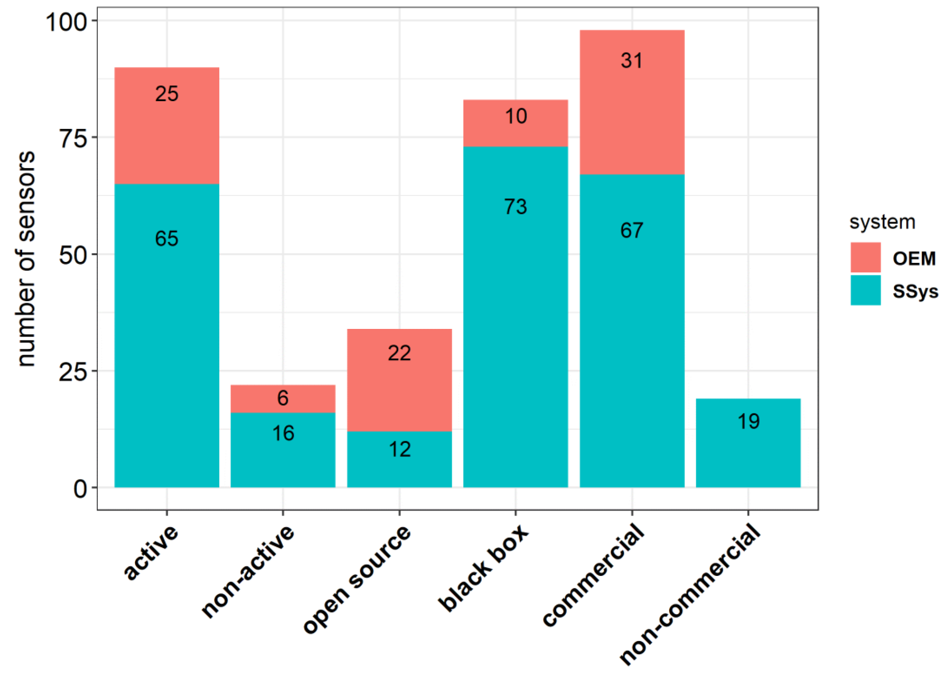
Figure 1. Number of LCS models gathered from the literature review highlighting their open data treatment (open source vs. black box) and commercial availability.
Atmosphere 10 00506 g001
Figure 2. Number of references per year of publication that includes quantitative comparison of sensor data with reference measurements. For 2019, the number of publications covers the publications from the period between January and April.
Atmosphere 10 00506 g002
Figure 3. Mean R2 found for LCS reporting calibration against reference measurements for all used calibration methods. The author name below each bullet gives the first author of the publication from which results were drawn.
Atmosphere 10 00506 g003
Figure 4. Mean R2 obtained from the comparison of SSys against reference measurements at all averaging times (1 min, 5 min, 1 h, and 24 h). The author name below each bullet gives the first author of the publication from which results were drawn.
Atmosphere 10 00506 g004
Figure 5. Prices of SSys grouped by model. Numbers on the right indicate the number of pollutants measured by each SSys, with open source in blue and black box in black. The x-axis uses a logarithmic scale. Names of “living” and “non-living” SSys are indicated in black and red colors on the labels of the y-axis, respectively. NC indicates commercially unavailable sensors.
Atmosphere 10 00506 g005
Figure 6. Price of low-cost SSys. Numbers in bold indicate the number of pollutants measured by open source (blue) and black box (black) sensors. Only records with R2 > 0.85 and 0.8 < slope < 1.2 are shown. Names of “living” and “updated” and “non-living” sensors are indicated in black and red on the labels of the x-axis, respectively. NC indicates commercially unavailable sensor. Labels reporting hourly/daily indicate the averaging time of reviewed records.
Atmosphere 10 00506 g006
Figure 7. Relationship between prices of LCS and R2 for field test only. A logarithmic scale has been set for both axes. Open source and black box models are indicated with red open dots and black solid dots, respectively. Names of “living” and “non-living” sensors are indicated by black and blue colors, respectively. R2 refers to data averaged over 1 h. Grey shade in the fit plots indicate a pointwise 95% confidence interval on the fitted values.
Atmosphere 10 00506 g007
Figure 8. Correspondence between R2 and slope for SSys. Only SSys models with R² > 0.75 and 0.5 < slope < 1.2 are shown. Names of “living” and “non-living” sensors are indicated in black and blue colors, respectively.
Atmosphere 10 00506 g008
Table 1. Number of analyzed “records” for LCS by pollutant and by type of technology.
PollutantTypen. Records Fieldn. Records LaboratoryReferences
COelectrochemical519AQ-SPEC [19], Jiao [39], Sun [40], Marjovi [57], Karagulian [22], Mead [44], Popoola [45], Borrego [53], Castell [10], Cross [58], Gerboles [23], Wei [59], Gillooly [60], Zimmerman [61], Spinelle [24,27]
COMOs272AQ-SPEC [19], Piedrahita [62], Spinelle [24]
NOelectrochemical446Jiao [39], Bigi [42], Karagulian [22], Mead [44], Popoola [45], AQ-SPEC [19], Castell [10], Borrego [53], Cross [58], Gillooly [60], Spinelle [24], Gerboles [23], Wei [59], Crunaire [33]
NOMOs1-Crunaire [33]
NO2electrochemical13721AQ-SPEC [19], Jiao [39], Williams [30], Sun [40], Mijling [41], Vaughn [32], Spinelle [20], Mueller [43], Bigi [42], Marjovi [57], Cordero [63], Karagulian [22], Mead [44], Popoola [45], Borrego [53], Castell [10], Cross [58], Spinelle [26], Duvall [64], Gillooly [60], Gerboles [23], Wei [59], Sun [65], Zimmerman [61], Lin [66], Crunaire [33]
NO2MOs2810AQ-SPEC [19], Vaughn [32], Williams [30], US-EPA [67], Borrego [53], Piedrahita [62], Spinelle [20], Crunaire [33]
O3electrochemical6510AQ-SPEC [19], Jiao [39], Spinelle [20], Mueller [43], Marjovi [57], Karagulian [22], Borrego [53], Castell [10], Cross [58], Duvall [64], Feinberg [36], Gerboles [23], Wei [59], Crunaire [33]
O3MOs543AQ-SPEC [19],Jiao [39], Spinelle [20], Borrego [53], Feinberg [36]
O3UV91Sun [40], AQ-SPEC [19]
PM2.5Electrical6-AQ-SPEC [19]
PM2.5nephelometer12924AQ-SPEC [19]], Borghi [37], Jiao [39], Feinberg [36], US-EPA [67], Williams [31], Manikonda [54], Zikova [55], Wang [68], Alvarado [69], Chakrabarti [70], Sousan [56],Borrego [53], Olivares [71],Sun [40], Pillarisetti [72], Holstius [51], Austin [73], Gao [74], Kelly [75], Karagulian [28], Badura [49], Crunaire [33]
PM2.5OPC42827AQ-SPEC [19], Mukherjee [35], Feinberg [36], Jiao [39], Cavaliere [76], Borrego [53], Viana [77], Williams [31], Manikonda [54], Northcross [78], Holstius [51], Steinle [79], Han [80], Jovasevic [81], Dacunto [82], Gillooly [60], Sousan [83], Crilley [84], Badura [49], Kelly [75], Zheng [85], Laquai [48], Budde [47], Liu [52], Crunaire [33]
PM1Electrical6-AQ-SPEC [19]
PM1nephelometer1-Crunaire [33]
PM1OPC1028AQ-SPEC [19], Williams [31], Sousan [83], Crilley [84], Crunaire [33]
PM10nephelometer261AQ-SPEC [19], Borrego [53], Alvarado [69], Crunaire [33]
PM10OPC17611AQ-SPEC [19], Cavaliere [76], Borrego [53], Feinberg [36], Manikonda [54], Sousan [56], Han [80], Jovasevic [81], Williams [31], Sousan [83], Crilley [84], Budde [47], Crunaire [33]
Table 2. Number of records gathered by metrics available in literature.
Metricsn. Field Testsn. Laboratory Tests
Total tests1290133
R², calibrations21860
R², comparisons116072
slope of regression line106355
intercept102754
RMSE2855
Measurement uncertainty (U)15329
MAE400
Bias193
Table 3. Types of calibration models used for the calibration of LCS.
PollutantCalibration Modeln. RecordsReferencesMedian R2 CalibrationMedian R2 Comparison
COANN2Wastine [94], Spinelle [24]-0.58
COlinear12Sun [40], Wastine [94], Castell [10], Cross [58], Gerboles [23], Spinelle [24], Zimmerman [61]0.850.15
COMLR21Jiao [39], Karagulian [22], Wastine [94], Wei [59], Piedrahita [62], Spinelle [24], Zimmerman [61]0.890.83
COquad12AQ-SPEC [19]0.63-
CORF1Zimmerman [61]0.91-
NOANN2Wastine [94], Spinelle [24]-0.57
NOlinear8Wastine [94], Castell [10], Cross [58], Spinelle [24], Karagulian [22], Crunaire [33]0.960.032
NOMLR20Jiao [39], Bigi [42], Karagulian [22], Wastine [94], Spinelle [24], Wei [59]0.920.91
NORF2Bigi [42]-0.9
NOSVR2Bigi [42]-0.90
NO2ANN7Cordero [63], Spinelle [20], Wastine [94], Wastine [95]0.870.94
NO2linear25Sun [40], Spinelle [20], Wastine [94], Wastine [95], Castell [10], Cross [58], Karagulian [22], Zimmerman [61], Lin [66], Crunaire [33]0.250.17
NO2log1Vaughn [32]0.89-
NO2MLR48Jiao [39], Sun [65], Mijling [41], Spinelle [20], Mueller [43], Bigi [42], Cordero [63], Karagulian [22], Wastine [94], Wastine [95], Piedrahita [62], Wei [59], Zimmerman [61]0.810.81
NO2quad6AQ-SPEC [19]0.61-
NO2RF7Bigi [42], Cordero [63], Zimmerman [61]0.860.91
NO2SVM4Cordero [63]0.850.94
NO2SVR2Bigi [42]-0.78
O3ANN2Spinelle [20], Wastine [94]-0.89
O3linear13Sun [40], Spinelle [20], Wastine [94], Castell [10], Cross [58], Karagulian [22], AQ-SPEC [19], Crunaire [33]0.840.53
O3log1Vaughn [32]0.88-
O3MLR20Jiao [39], Spinelle [20], Karagulian [22], Wastine [94], Spinelle [25], Wei [59]0.910.88
O3quad9AQ-SPEC [19]0.72-
PM1Kholer2Di Antonio [96] -0.74
PM1log6AQ-SPEC [19]0.76-
PM10exp6AQ-SPEC [19]0.59-
PM10linear3Cavaliere [76], Jovanovic [81], AQ-SPEC [19]0.770.73
PM10log7AQ-SPEC [19]0.58-
PM10quad1Alvarado [69]0.65-
PM10-2.5linear4Sousan [56], Han [80], Jovasevic [81]0.630.98
PM2.5exp3Dacunto [82], Kelly [75], Austin [73]0.910.97
PM2.5Kholer2Crilley [84], Di Antonio [96] -0.78
PM2.5linear37Mukherjee [35], Wang [68], Alvarado [69], Cavaliere [76], Jovasevic [81], Olivares [71], Kelly [75], Zheng [85], Holstius [51]0.840.64
PM2.5log7AQ-SPEC [19], Laquai [48]0.73-
PM2.5MLR17Jiao [39], Sun [65], Zheng [85], Holstius [51], Liu [52]0.810.65
PM2.5quad8Chakrabarti [70], Alvarado [69], Zheng [85] Gao [74]0.870.88
PM2.5RF3Liu [52]-0.79
PM2.5–0.5linear9Northcross [78], Steinle [79], Han [80], Jovasevic [81]0.840.98
PM2.5–0.5MLR1Jiao [39]0.60.45
PM2.5–0.5quad6AQ-SPEC [19], Manikonda [54]0.82-
Note: ANN = artificial neural network; exp = exponential; log = logarithmic; MLR = multilinear regression; quad = quadratic; RF = random forest; SVM = support vector machine; SVR = support vector regression; Kohler = particle size distribution-based correction algorithm accounting for the influence of relative humidity.
Table 4. Shortlist of SSys showing good agreement with reference systems (R2 > 0.85; 0.8 < slope < 1.2) for 1 h time-averaged data.
ModelPollutantMean R²Mean SlopeMean Absolute InterceptOpen/CloseLivingCommercialPrice (EUR)
AirNutPM2.50.860.888.6black boxYcommercial132
PA-IPM10.950.920.52black boxNcommercial132
PA-IIPM10.990.821.8black boxYcommercial176
Egg (2018)PM10.870.850.095black boxYcommercial219
PATS+PM2.50.960.920.05black boxYcommercial440
S-500NO2, O30.880.970.27black boxYcommercial440
CairClip O3/NO2O30.880.8812black boxYcommercial600
Portable AS-LUNGPM10.890.871.0Black BoxYnon-commercial880
AirSensEUR (v.1)NO2, O3, CO, NO0.950.98-open sourceYcommercial1600
AirSensEUR (v.2)NO2, O3, CO, NO0.891.15.7open sourceYcommercial1600
Met One (NM)PM2.50.861.12.8black boxYcommercial1672
Air Quality StationPM10.880.900.85black boxYnon-commercial1760
AQY v0.5PM2.50.870.974.0black boxupdatedcommercial2640
Vaisala AQT410 v.1.15CO0.870.970.23black boxYcommercial3256
2B Tech. (POM) *O31.001.000.74black boxYcommercial3960
AQMesh v.3.0NO0.870.880.76black boxNcommercial8800
Note: * The 2B Tech. (POM) is a miniaturized reference method, UV photometry, which explains the perfect R² And slope of 1.