Ammonia Emissions Measured Using Two Different GasFinder Open-Path Lasers

Abstract

The challenges of accurately measuring in situ ammonia (NH₃) losses from agricultural systems are well known. Using an open path laser coupled with a backward Lagrangian stochastic dispersion model is a promising approach for quantifying both point- and area-sources; however, this approach requires the open path laser to detect low NH₃ concentrations and small concentration differences. In this study, we compared the new GasFinder3 open path laser (Boreal laser Inc., Edmonton, Canada) with the GasFinder2 sensor, the previous version. The study took place at two locations: an outdoor open-air manure compost site, and a field of wheat stubble which was fertilized with urea ammonium nitrate. Results showed the two lasers reported similar concentrations during three days of measurements at the compost site, but differed at the field site, where concentrations were close to the minimum detection limit. The GasFinder3 had a lower standard deviation under all conditions, especially with low wind speed and high relative humidity.

1. Introduction

The agriculture sector contributes up to 80% of global NH₃ emissions [1], which are emitted mainly from the field application of nitrogen from inorganic fertilizer and organic material (e.g., livestock manure, compost). These emissions may be detrimental to human health and to natural ecosystems both locally and via long-range atmospheric transport [2]. Identifying agricultural practices that mitigate NH₃ emissions requires the accurate quantification of NH₃ emissions under real-world conditions.

Measurements of NH₃ emissions from agriculture have often been done using chambers or “wind-tunnels” deployed on small experimental plots (typically ≤1 m²) designed to compare treatments over a number of days [3]. The most common micrometeorological method has been the Integrated Horizontal Flux method, which is non-disruptive but requires a circular plot, which limits its flexibility for studying farm-scale practices. Micrometeorological methods, such as the backward Lagrangian dispersion method (bLS) [4], enable the measurement of NH₃ losses from point sources and area sources, with little constraint to either shape or size.

Research using the bLS method often employs open path tunable diode lasers to measure NH₃ concentration up- and down-wind of the source (e.g., [5,6,7,8,9]). This method was successfully tested at the field scale for estimating NH₃ emission [8]. Important challenges of using bLS to measure NH₃ emissions are that ambient NH₃ concentrations are near zero and that NH₃ fluxes change rapidly and exhibit a large range (e.g., high emissions after manure application decline to near zero within a few days). It is unclear whether the open path tunable laser coupled with the backward Lagrangian stochastic (OPTDL-BLS) dispersion technique underestimates or overestimates the low flux of NH₃ losses. Ni et al. [7] found that, among the 4 approaches tested in their study, the OPTDL-BLS technique had the highest sensitivity at low concentrations; on the other hand, Yang et al. [8] found that the OPTDL-BLS technique was unable to estimate low NH₃ flux. This inconsistency between the two studies may be linked to the ability of the lasers used for measuring low NH₃ concentrations [8].

According to the manufacturer (Boreal Laser, Edmonton, AB, Canada), the newly released GasFinder3 (GF3) open path laser [10] has several improvements relative to the previous version (GasFinder2; GF2) that may improve its accuracy at low concentrations [11]. The GasFinder3 has precise temperature control of the laser (within 0.005 °C) and instrument, which enables it to stay in calibration over a wider ambient temperature range (−40 °C to +50 °C) while also improving measurement sensitivity and stability. A major change in the GasFinder3 is the use of digital signal processing (whereas the GasFinder2 uses analog). This change enables multiple analysis algorithms to be used, including wavelength modulation spectroscopy for low to high gas concentrations, which greatly increases the dynamic measurement range. Changes to the optical design of the GasFinder3 and its reflectors are intended to reduce optical noise, which further improves measurement stability.

The objective of this study was to compare the GF3 and GF2 for measuring NH₃ losses from different agricultural practices (composting system, fertilizer application) and different source intensities (ambient, low and high levels).

2. Experiments

2.1. Description of GasFinder Open Path Laser

The GasFinder (2 and 3) open path (OP) lasers consist of an integrated transmitter/receiver unit and a remote reflector [10,11]. The OP laser is mounted on a tripod and aimed at the reflector array. The transceiver includes a detector, a micro-computer and a distributed feedback diode laser operated in continuous wave output, with a typical power output of 10 mW and bandwidth of 2 MHz. Interferences with nearby gases are avoided by using the 1512.2 nm absorption line, which operates away from the absorption of interfering gases including water vapour. The laser emits a beam that propagates through the atmosphere to the retroreflector array that reflects the beam back to a photodiode detector. At the same time, a laser beam is passed through an onboard gas cell to provide a reference signal. The two optical signals are converted into a waveform which is processed by the microcontroller to determine the concentration of the target gas along the path-length. The gas concentrations are measured and recorded as the path-integrated concentration (in parts per million meters, ppm*m or ppmm), which can be converted to the path-average concentration (in parts per million, ppm) by dividing by the path-length (m) measured by the operator. In addition to concentration, the sensors calculate an R² parameter associated with each measurement, which is the result of a linear regression of the sample and calibration waveforms (R² range: 0 to 100%). A low R² is associated with a low path-integrated concentration of the target gas in the sample air. The sensors also record a light-level parameter that responds to the amount of received power. The GF2 uses a 14 bit analog-to-digital converter, while the GF3 uses 18 bits. For the GF2, the light level has a dimensionless scale from zero to 16,384 (the GF2 detector saturates around 300 µW). For the GF3, light level is termed “Rx” (received power), which is measured and recorded in microwatts (the manufacturer-recommended operating range is between 50 and 3000 µW). Data are collected, stored, and displayed in the same format for both lasers (GF2 and GF3). More information and a description of GasFinder characteristics can be obtained from the manufacturer [10,11].

2.2. Experiemtal Sites, Sensor Installations and Data Acquisition

To evaluate the performance of the GasFinder3 (GF3, NH3OP-30004, Software V1.0.5c.b5) compared to the GasFinder2 (GF2, NH3OP-1038, Coldfire Processor V1.10.h), the lasers were simultaneously calibrated side-by-side by the manufacturer. Calibration involved aiming each laser through a transparent cylinder, 1.5 m in length, with a reflector on the opposite end. According to the manufacturer, the gas concentration within the cylinder was controlled using a multi-component gas mixing system (Series 4000; Environics, Inc., Tolland, CT, USA) that was calibrated with National Institute of Standards and Technology (NIST) traceable flow standards. Calibration was performed using compressed nitrogen (Grade 5.0; Linde Canada, Ltd., Edmonton, AB, Canada) as the diluent gas and certified NH₃ cylinders with concentrations of 306.2 ppm and 0.55% (Linde Canada, Ltd., Edmonton, AB, Canada). Since NH₃ is a sticky gas, a small amount of hydrogen fluoride gas was flowed through the transparent calibration cylinder at the start of the calibration process to remove NH₃; this was followed by purging with N₂ to obtain a zero concentration. During the calibration, concentrations were increased incrementally, and ample time was given for the concentration to stabilize after each concentration change. Raw data from the calibration at 5, 25, and 50 ppmm were used to calculate the minimum detection limit for each laser following this [12]. The minimum detection limits were determined to be 2.4 ppmm for the GF2 and 2.2 ppmm for the GF3.

During the study, lasers were set up side-by-side to measure NH₃ concentrations at two sites that represent important agricultural emission sources; i.e., manure management and fertilized fields. The first study was at a manure composting facility, and the second site was a field that was fertilized after wheat harvest.

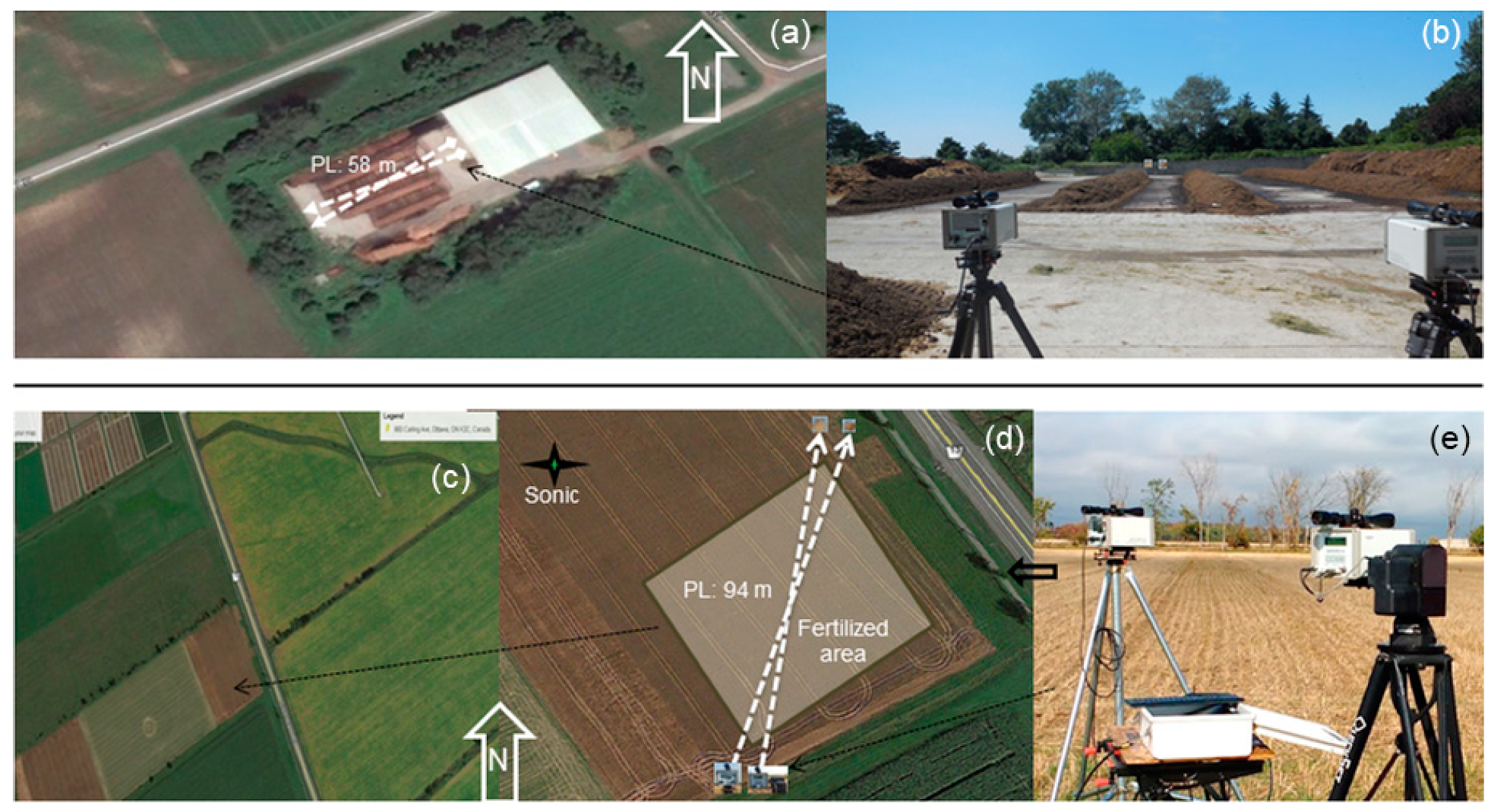
2.2.1. NH₃ Measurements at Outdoor Manure Compost Windrows

Solid dairy manure was composted in windrows on a concrete pad with 2 m high walls on three sides. This was located in a field at the Central Experimental Farm (CEF, Ottawa, ON, Canada) (Figure 1). Concentrations of NH₃ were measured during three days in summer: 27 July 2017 from 9:00 a.m. to 4:00 p.m. (noted D1), 28 July from 9:00 a.m. to 3:00 p.m. (D2), and 1 August from 9:00 a.m. to 3:00 p.m. (D3). Lasers and retro-reflectors were mounted on tripods at 1.5 m height between two compost piles (Figure 1b). The path-length between each laser–reflector pair was 58 m (Figure 1a). To avoid interference between sensors, a 2 m space was provided between lasers and between reflectors. To provide a similar measurement path, laser paths were oriented crosswise so the beams crossed at 29 m. Retro-reflector arrays consisted of 7 corner-cubes that reflect light back to the source, regardless of the angle of incidence. The arrays had a thin polycarbonate window material. To reduce the intensity of the reflected signal to the desired range (i.e., light level) for the GF2 detector, the retro-reflector array was covered by a mesh screen (24 × 24, i.e., 24 wires per inch; Stainless Steel Mesh, Gerrard Daniel Worldwide, Mississauga, Ontario, Canada) placed between the corner-cubes and the polycarbonate. No mesh screen was needed for the GF3 as it is not sensitive to a high return light signal.

Lasers were turned on overnight, prior to the start of measurements each day, to ensure the internal temperature control was stabilized. Lasers were internally set to sample and record data in “real time” mode, which records data every 1–2 seconds (i.e., 500 sweeps over the absorption feature for GF3 and 512 sweeps for GF2). Both GF2 and GF3 data were corrected for ambient temperature and pressure during post-processing using the manufacturer-supplied calibration curves. The GF3 sensor has the capability to apply these corrections in real-time using an internal pressure sensor and external temperature sensor; however, we did not use this feature. Although the GF3 has better internal temperature control, these corrections are required to address the spectroscopy-related effects of changes in atmospheric temperature and pressure in the laser path. Meteorological data, including air temperature (minimum, maximum and mean), solar radiation, relative humidity, and wind speed, were collected as hourly averages from a nearby weather station (Ottawa CDA, Climate ID 6105976) about 500 m away (

Table 1. Hourly averaged air temperature, solar radiation, wind speed and relative humidity measured from the weather station near the composter.

Date	Hour	Air Temperature	Solar Radiation	Wind Speed	Wind Direction	Relative Humidity
	Eastern Time	°C	MJ m−2	m s−1	°	%
2017-07-27	10	21.6	2.1	4.4	297	73
	11	21.7	1.5	4.9	290	71
	12	21.4	1.2	5.0	279	70
	13	22.7	2.8	4.8	268	66
	Average	21.9	1.9	4.8	284	70
2017-07-28	9	16.6	2.2	3.7	338	61
	10	17.7	2.8	3.7	328	55
	11	18.8	3.1	4.6	337	42
	12	20	3.1	4.2	176	39
	13	20.9	3.3	5.0	348	39
	14	21.5	3.1	4.5	337	40
	Average	19.3	2.9	4.3	311	46
2017-08-01	9	22.6	2.1	0.8	85	54
	10	24.3	2.6	0.6	186	44
	11	25.3	3.0	0.9	75	43
	12	26.2	3.2	1.4	196	37
	13	27	3.2	2.6	208	38
	14	27.6	3.1	2.1	197	41
	Average	25.5	2.9	1.4	157.8	42.8

). Fluxes were not calculated because the site configuration was too complex for the bLS technique (due to nearby trees and walls). Therefore, data analysis at this site was focused on evaluating the consistency of concentration measurements by the lasers (GF3 vs GF2) over a range of concentrations (ambient, low and high concentration).

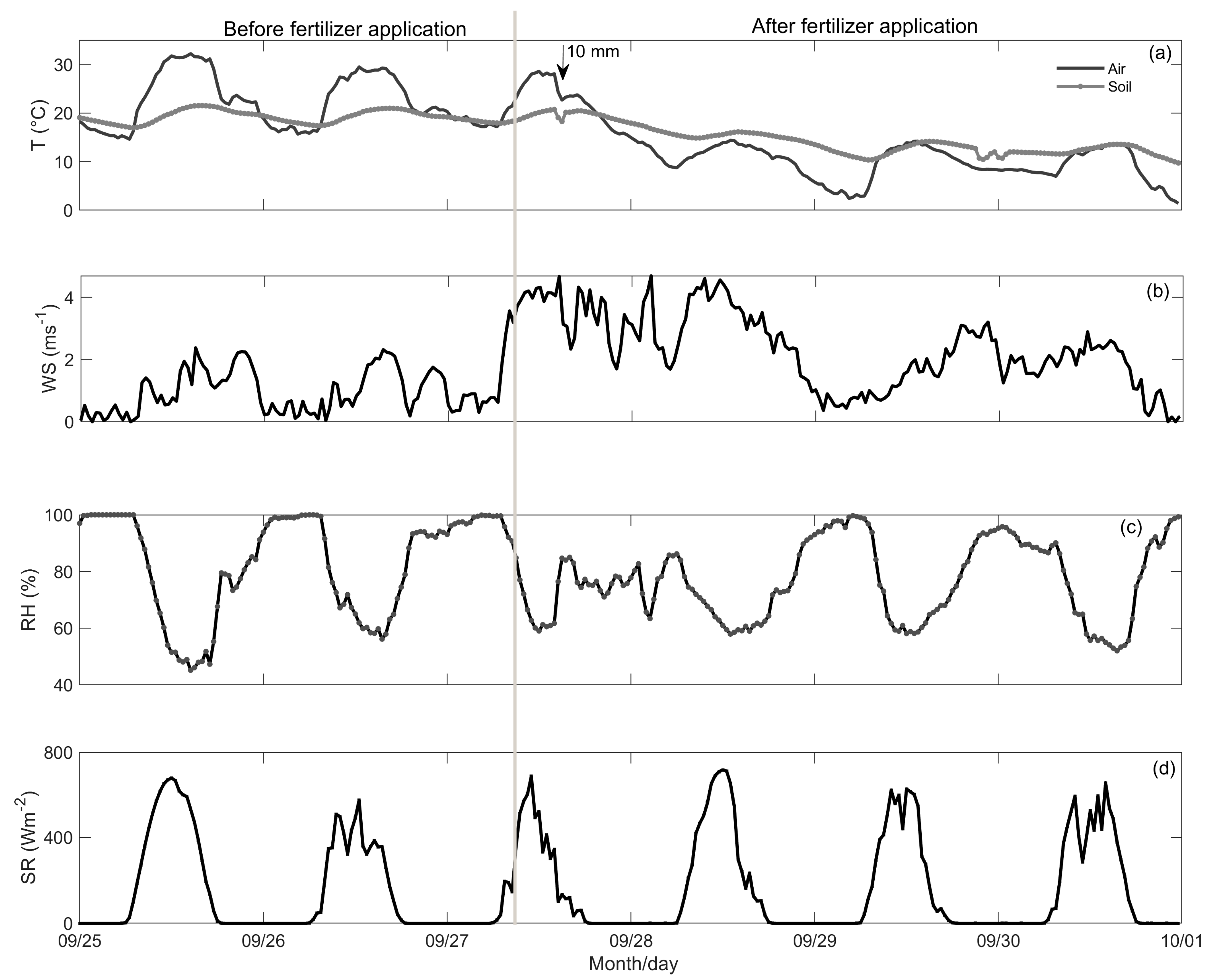
2.2.2. NH₃ Measurements from Fertilized Wheat Stubble

The field trial was located at the Canadian Food Inspection Agency experimental farm in Ottawa, about 10 km from the compost site (Figure 1c). An experimental plot of 60 m × 60 m was selected within a flat 3 ha field of wheat stubble (Figure 1d). The soil texture was silt loam with 29% sand, 54% silt and 16% clay; organic matter was 4.6 ± 0.2% and pH was 6.2 ± 0.1, on average (n = 27). Measurements occurred from 21 September to 11 October 2017 using the same lasers (GF3, NH3-OP30004; GF2, NH3-OP1038), two reflectors, a 3D sonic anemometer, tripods, and a field computer. Lasers were positioned to measure NH₃ concentration diagonally across the plot (Figure 1d). Therefore, lasers were set up side-by-side at the south-west corner of the plot, targeting two reflectors located diagonally across the plot (north-east corner). The separation distance between the pairs of lasers and pairs of reflectors was at least 2 m. The path length was 94 m for both lasers, and the height of all lasers and reflectors was 1.5 m. Lasers and reflectors were placed 2 m outside the edge of the fertilized area. Both reflectors had 12 corner-cubes with thin polycarbonate window material on the enclosures. In addition, the GF2 had a mesh screen placed inside the reflector, as described in Section 2.2.1.

The field site was flat, with no obstructions and no other NH₃ sources upwind (i.e., no livestock, no manure, and no other fields were fertilized for the preceding ~2 months). Therefore, the source was well defined and the site was well suited to calculate emission rates using the bLS technique.

To determine NH₃ emissions, the bLS technique requires both the NH₃ concentration measured from open-path lasers and wind turbulence data. Turbulence data were measured using a three-dimensional sonic anemometer (CSAT3, Campbell Scientific, Inc., Logan, Utah) at 1.5 m height (Figure 1d). Additional meteorological data, including air and soil temperature, relative humidity, wind speed and direction, solar radiation and rainfall, were measured at a weather station located in the adjacent field (about 200 m away).

Ambient (background) NH₃ concentration before fertilizer application was measured from 21 to 27 September. On 27 September, around 9:30 a.m., urea ammonium nitrate (UAN; 28%) was applied homogeneously on the surface of the 3600 m² plot by the farm operator using a sprayer boom. Unfortunately, it was not possible to determine the quantity of fertilizer applied. The field was covered with wheat stubble (less than 10 cm height) after grain and straw was harvested early in September.

2.3. Data Processing

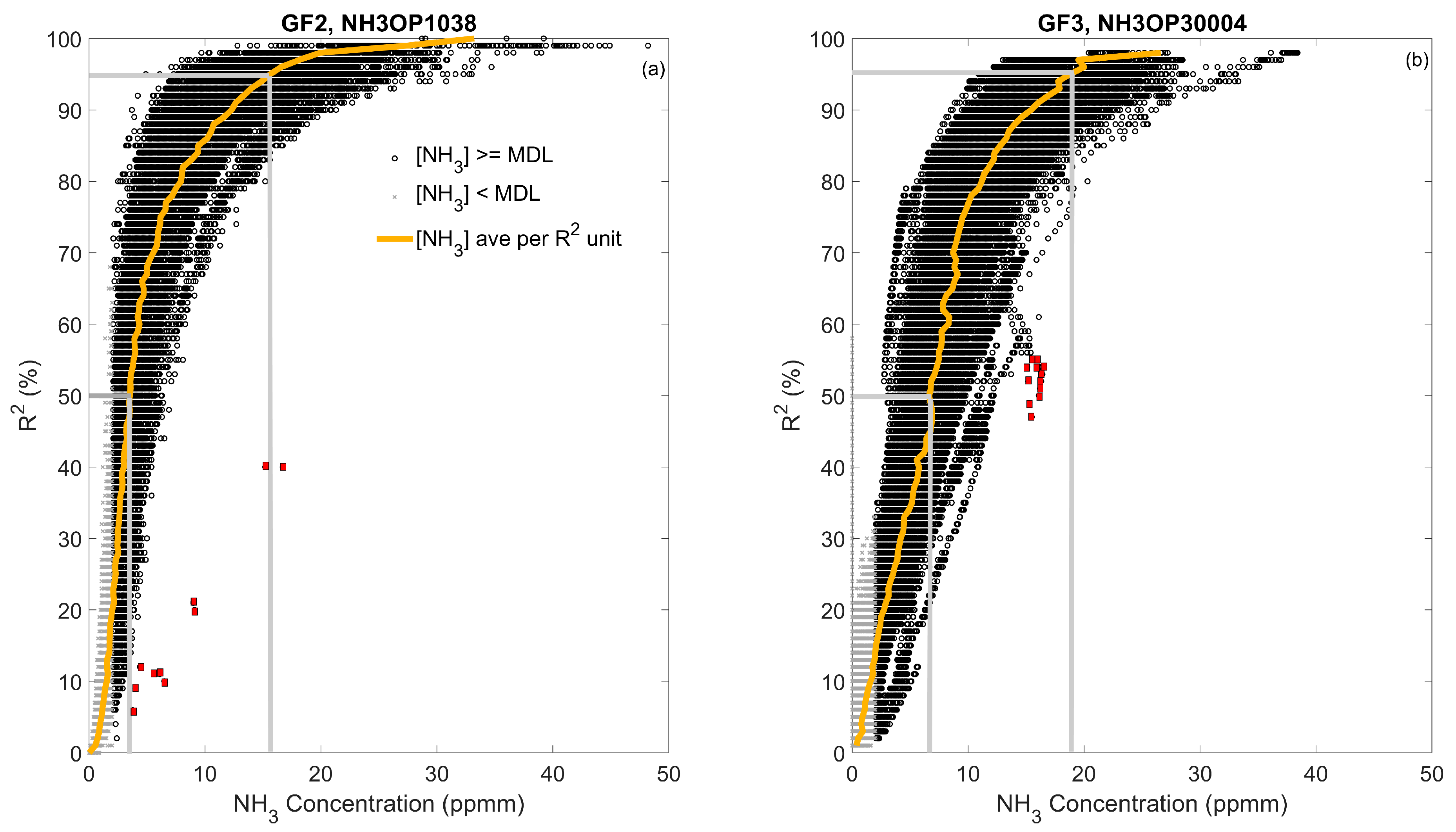
2.3.1. NH₃ Concentration Data Processing

Both lasers recorded data in an ASCII string format with an identical number of columns: (i) NH₃ concentration (ppmm), (ii) R² between reference and sample signals (unitless percent), (iii) path length (m), (iv) light level (for GF2) and Rx (for GF3) returned from the reflector (unitless integer), (v) date and time, (vi) laser serial number, and vii) the status code of system operation.

Preliminary filters were applied on the raw NH₃ concentration to keep data when the lasers were operating normally (status code = 1) and had an appropriate light level (>4000 and <15,000, for GF2) and Rx level (>200 and <2500, for GF3; note that the measured Rx never reached 2500). Values below the minimum detection limit were removed. The graph of concentration (ppmm) vs R² was plotted to observe the shape of the curves in order to identify possible outliers for manual removal as recommended by manufacturer. After those filters, concentration data were averaged in 1 min periods. Descriptive statistics were calculated from the binned data to calculate the mean, median, minimum, maximum, standard deviations and the number of observations (after filtering) within each 1 min period. Only periods with more than 30 observations per bin were kept for analysis. The Allan variance was calculated using raw concentration data measured before fertilizer application at the field. Furthermore, measured NH₃ concentrations were analyzed relative to the observed meteorological parameters to identify the influence of these parameters.

To compare the two lasers, data from each laser were summarized (means and standard deviations) in 1 min periods and then synchronized. Only periods when both lasers had valid data were retained for further analysis. In addition to descriptive statistics of the difference between the two lasers (GF2–GF3), paired t-tests or Wilcoxon signed-rank tests (when the data was not normally distributed) were used on paired 1 min data to test whether the difference between means were significantly different from zero.

Analyses at the composter site were done on each of the three days and over all three days combined. At the field site, data were grouped into two time periods: before and after fertilizer application.

2.3.2. Calculating NH₃ Emission Rates

The bLS technique was used to determine NH₃ emissions in our field study using WindTrax software (model Version 2.0.8.9, Thunder Beach Scientific, Edmonton, AB, Canada). Two sets of emission data were calculated using the GF2 and GF3 lasers. In each case, concentration data from each laser were synchronized in 15 min bins with wind turbulence data from the sonic anemometer to create input files for WindTrax. The NH₃ background concentration measured by the GF3 before fertilizer application was 0.001 ppm (median = 0), which is below the minimum detection limit reported [13] for a GF2 of 2 ppmm; i.e., 0.021 ppm on a 94 m path length. Windtrax simulations used a background concentration of zero. This is consistent with several studies (e.g., [7,9]). Ni et al. [7] compared several field-scale methodologies including micrometeorological and chamber methods to measure NH₃ ammonia emissions after nitrogen fertilization and found that NH₃ background concentration ranged between 0 and 0.0076 ppm, which is below the minimum detection limit reported for a GF2 (0.024 ppm = 5.34 ppmm on a 220 m path length) by the USEPA [14].

The accuracy of NH₃ emission calculations using bLS model depends on atmospheric turbulence as described by Monin–Obukhov similarity theory (MOST) [15]. Therefore, filters were applied to friction velocity (u*), Monin–Obukhov length (L), and surface roughness (Z₀) calculated by Windtrax to remove data when u* < 0.15 m s⁻¹, |L| < 5 m, or Z₀ > 0.25 m. Then, data from both lasers were synchronized (on a 15 min basis) and analyses were made on filtered NH₃ concentration and emission rates.

Cumulative emissions over the 88 h of measurement after fertilization were calculated from hourly averaged emissions with a linear interpolation to fill missing hours. Comparisons between the lasers were performed using paired-comparison t-tests on filtered NH₃ concentrations and emission rates before and after fertilizer application.

3. Results and Discussion

3.1. Environmental Data

During measurements at the compost site, average air temperatures ranged from 19.3 °C on day 2 (D2) to 25.5 °C on D3 (Table 1). Averaged solar radiation were similar on D2 and D3 (2.9 MJ m⁻² h⁻¹), and lower on D1 (1.9 MJ m⁻² h⁻¹). Mean relative humidity was higher on D1 (70%) compared to D2 (46%) and D3 (43%). Averaged wind speed and direction were similar on D1 (4.8 m s⁻¹, 311°) and D2 (4.3 m s⁻¹, 283°), but not D3 (1.4 m s⁻¹, 158°) (Table 1).

During the field trial, a significant change in weather occurred 6 h after fertilizer application when a brief and intense storm delivered 10 mm of rain in under 15 min, accompanied by strong winds (Figure 2). On average, the air and soil temperatures were higher before fertilizer application (22.2 and 19.2 °C, respectively) than after fertilizer application (12.2 and 14.4 °C, respectively). In contrast, the average wind speed was lower (1.0 m s⁻¹) before fertilization than after (2.4 m s⁻¹) (Figure 2b). Solar radiation was higher after fertilization (172 W m⁻²) than before (151 W m⁻²) on average (Figure 2d). Relative humidity was somewhat higher (83%) before fertilization than after (76%) on average (Figure 2c). Soil moisture increased after the rain storm, but declined slightly on average, from 35% before application to 33% after fertilizer application (not shown).

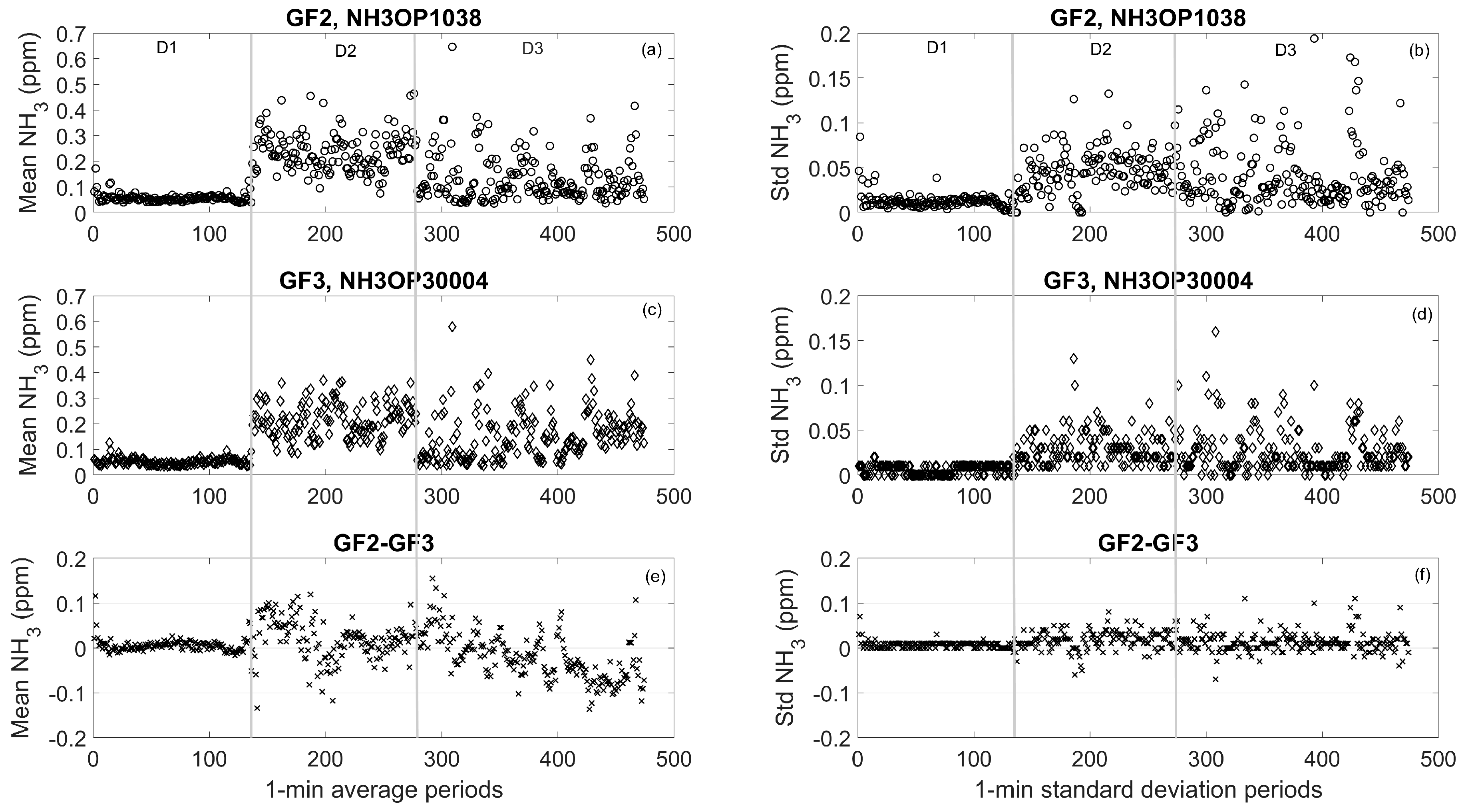
3.2. NH₃ Concentrations Measured by GasFinder 2 & 3

3.2.1. NH₃ Concentrations at the Composting Facility

The relationship between NH₃ concentration and R² followed the characteristic pattern, increasing from zero (when no NH₃ was present) and approaching 100% as the concentration of NH₃ increased (Figure 3). The curves were not identical, however, as the GF2 approached maximum R² at a lower concentration than the GF3. For example, the GF2 reached R² = 50% at 3.53 ppmm, and R²= 95% at 15.63 ppmm, while the GF3 reached the same R² thresholds at 6.24 and 18.06 ppmm, respectively. While the difference between curves is notable, it does not indicate an advantage of one system over another. Differences could relate to either sensor design or differences between reflectors (mesh screen for GF2, no mesh for GF3). Both lasers had a small number of outliers from the curves, which were manually removed during data processing. Outliers can be seen in Figure 3, on the right of each curve (10 points removed for GF2, 12 removed for GF3).

As shown in Figure 4, NH₃ concentrations measured at the compost facility changed substantially from day to day. Averaged NH₃ concentrations increased over four-fold on the second day, being consistently observed by both lasers (Table 1 and

Table 2. Ratios of the means and standard deviations (σ) calculated on a 1 min basis of NH₃ concentrations over each measurement period. Averages are on daily basis (D1, D2 and D3) at the composter and before and after fertilizer application at the field trial. P-values from paired difference tests are shown.

Parameters	Sensor	Composting Facility				Wheat Stubble
		All Days	D1	D2	D3	Before Fertilizer	After Fertilizer
Mean [NH3] (ppm) 1 min periods	GF2	0.1417	0.057	0.235	0.134	0.054	0.062
	GF3	0.1418	0.052	0.216	0.152	0.034	0.041
	p-value	0.972	<0.001	<0.001	<0.001	0.034	<0.001
	n	474	136	139	199	18	736
Ratio: GF2/GF3		0.999	1.10	1.09	0.88	1.59	1.51
Mean 1 min σ (ppm)	GF2	0.034	0.013	0.048	0.040	0.018	0.024
	GF3	0.022	0.006	0.030	0.027	0.004	0.004
Ratio: GF2/GF3		1.55	2.17	1.60	1.48	4.50	6.00
σ/mean	GF2	24%	23%	20%	30%	33%	39%
	GF3	16%	12%	14%	18%	12%	10%
Mean NH3 Flux (g ha−1 h−1)	GF2		No flux calculation				4.34
	GF3						3.48
	p-value						<0.001
Ratio: GF2/GF3							1.25

, Figure 4a,c). Since there were no physical disruptions to the compost piles during the three days (i.e., no aeration or mixing), the temporal dynamics were tied to environmental conditions; specifically, D2 and D3 had high solar radiation (2.9 MJ m⁻² h⁻¹ on average, which would lead to greater surface temperature), and low relative humidity (43 to 46%). In contrast, D1 was cloudy. This agrees with previous research where solar radiation was the dominant factor influencing NH₃ emissions [8].

Comparing the Allan variance of the two lasers showed the GF2 reached a minimum at an averaging time of approximately 850 s, while the GF3 had a minimum at approximately 1000 s. Both of these results fit well with the 900 s (15 min) averaging time commonly used in bLS studies. The ratios (GF2/GF3) of mean NH₃ concentrations showed an overall ratio of 0.999 over the entire measurement period (Table 2). Although the ratio ranged from 0.88 (D3) to 1.10 (D1), there was not a significant difference (p = 0.97) in the mean concentration measured by the lasers over the three days. Averaged standard deviations within 1 min periods were from 1.5 to 2.1-times higher for the GF2 than the GF3, with an overall ratio of 1.58 (Table 2, Figure 4b,d). The difference was most pronounced during low concentrations on D1 (Table 2).

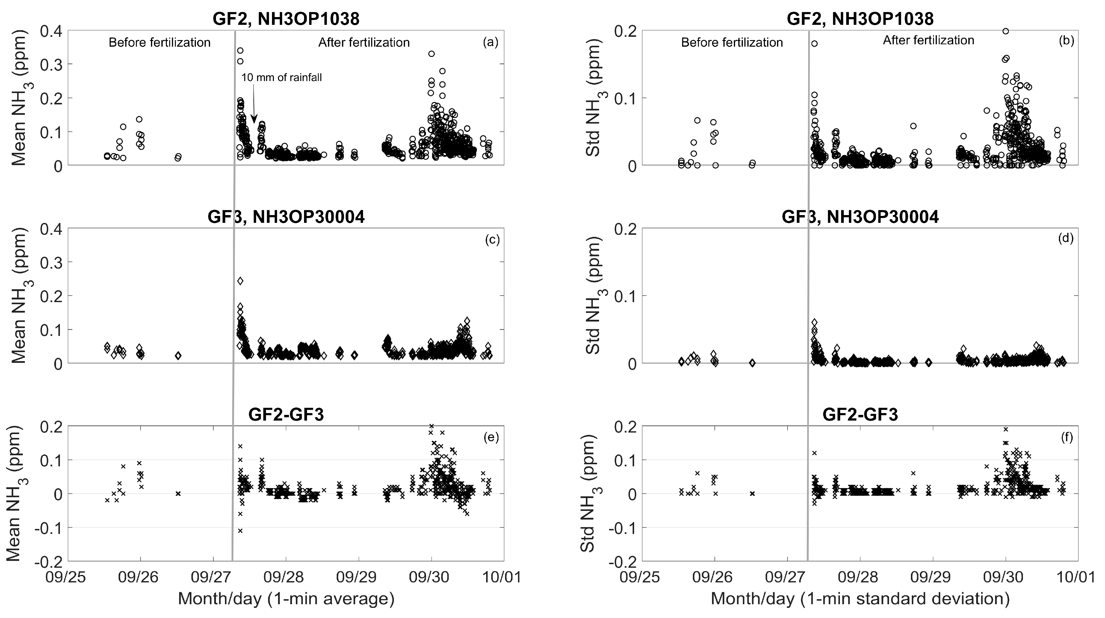
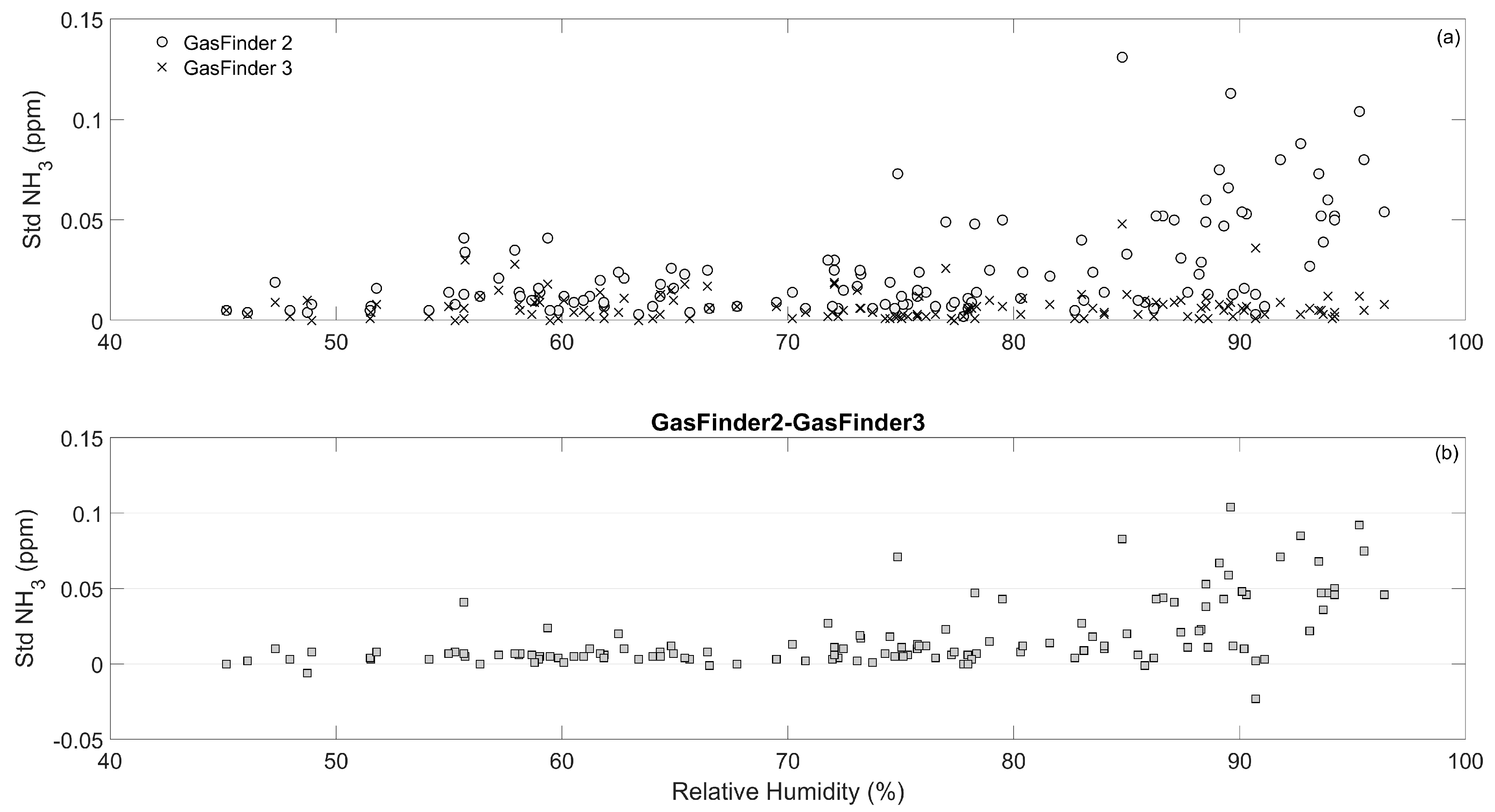
3.2.2. NH₃ Concentrations Measured at the Field Trial

Ammonia concentrations were measured for six days during the field trial. This included two days of near-background concentration (before fertilizer application), and four days of moderate concentrations after fertilization. Before fertilizer application, NH₃ concentrations were usually below the minimum detection limit for both lasers (Figure 5a,c). For the short periods of time with detectable concentrations, there was a significant difference between the lasers, as the GF2 was about 1.6 times higher than the GF3 on average (p < 0.05; Table 2). The standard deviation (σ) was also about 4.5 times higher for the GF2 than the GF3 (Table 2; Figure 5b,d).

After fertilizer application, NH₃ concentrations increased as expected but were generally lower than at the compost site. Concentrations measured by the two lasers were significantly different, with the GF2 reporting a roughly 1.5-fold higher concentration than the GF3 (p < 0.001) (Figure 5a,c, Table 2). The averaged σ (1 min period) after fertilizer application was 6 times higher for the GF2 than the GF3, and the coefficient of variation (σ/mean) was about 4 times higher for the GF2 (Figure 5b,d, Table 2).

The results suggest that the GF3 was more stable than the GF2 (lower σ, lower coefficient of variation). The analysis of environmental variables showed the difference in σ was particularly evident during conditions associated with high humidity (above ~85% RH; Figure 6). While our data do not address the underlying mechanism for this observation, they are consistent with the fact that the GF3 was improved in design for maintaining stable operation under a wide range of environmental conditions (e.g., precise internal temperature control; see US Patent US20160329681A1).

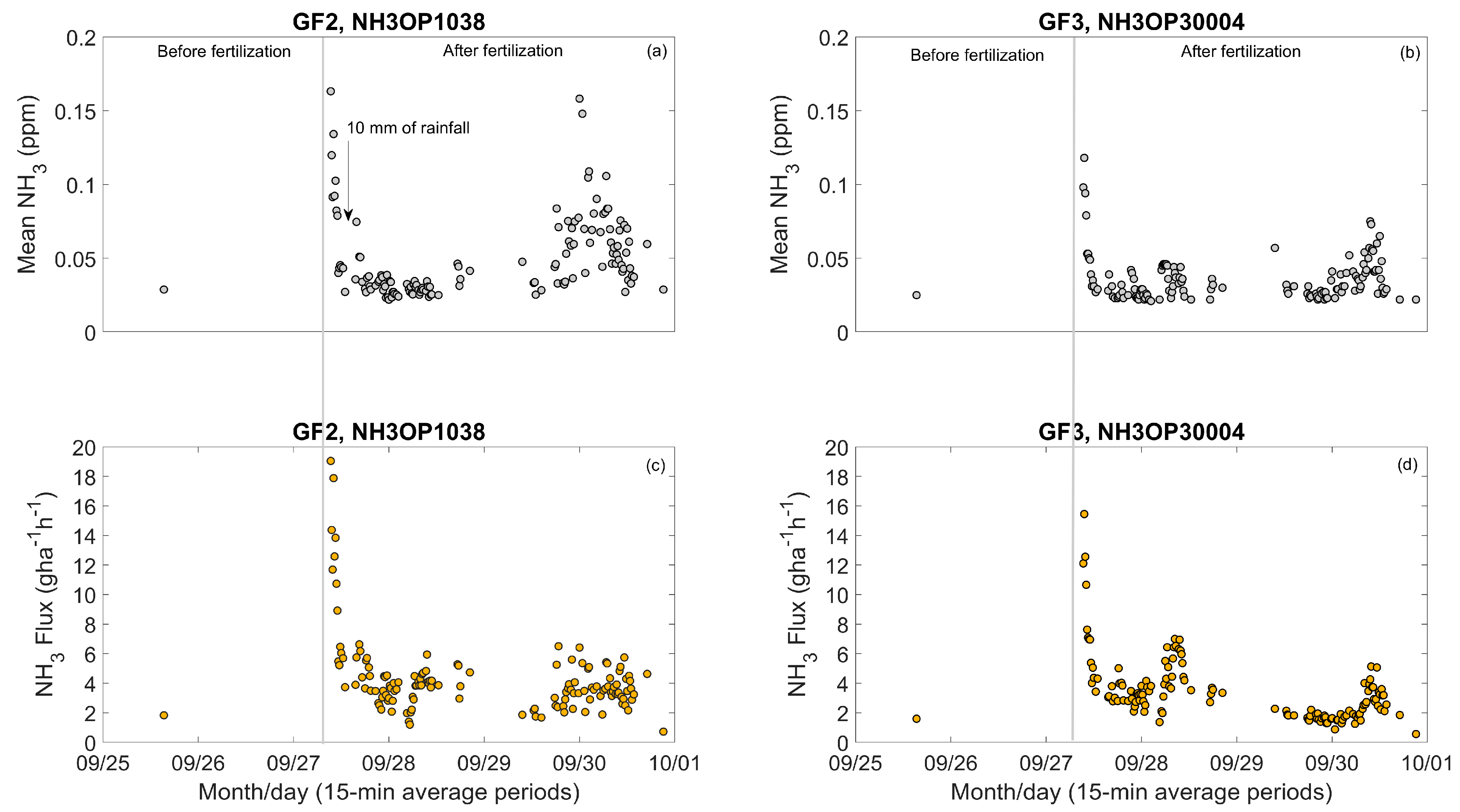
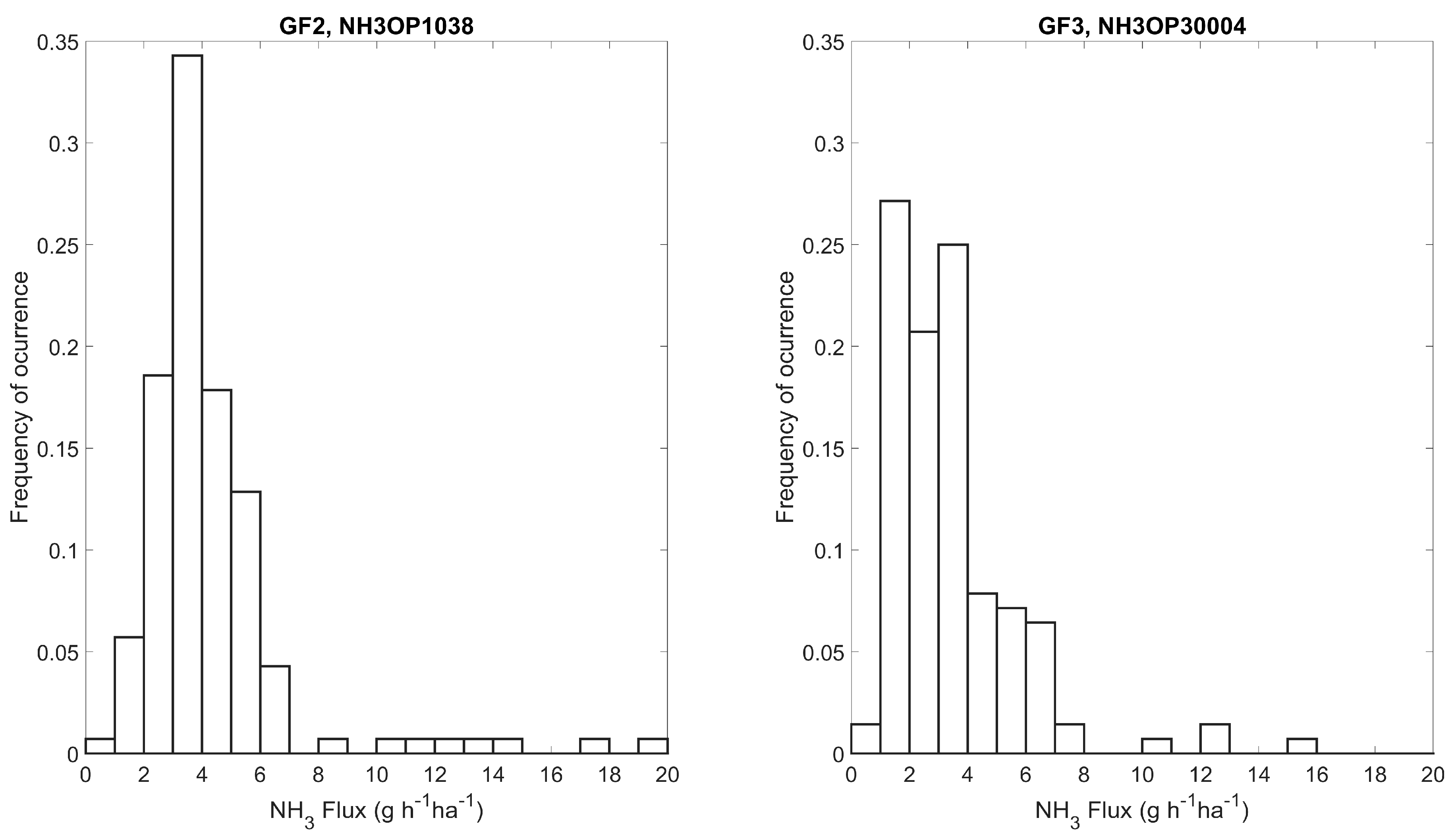
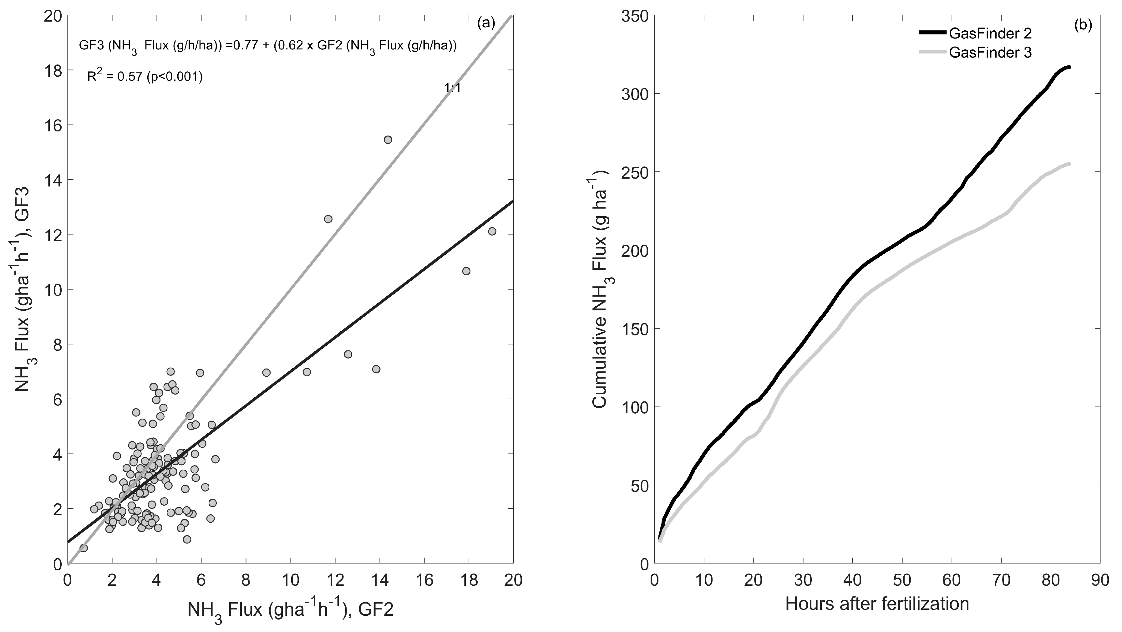
3.3. NH₃ Emissions at the Field Trial

After fertilizer application, NH₃ concentrations increased (Figure 7a,b), and fluxes increased to a maximum of 19.1 g ha⁻¹ h⁻¹ for the GF2 and 15.5 g ha⁻¹ h⁻¹ for the GF3 on a 15 min basis (Figure 7c,d). Soon after fertilization, however, those fluxes decreased rapidly, with most fluxes being under 8 g ha⁻¹ h⁻¹ (Figure 8). This was likely due to the application method (surface), the low rate of fertilizer applied, and the heavy rainfall. Despite the severe weather conditions (wind gusting up to 25 m s⁻¹), all sensors remained operational during and after the storm.

After fertilizer application (over about 88 h), NH₃ fluxes measured using the two lasers showed a significant correlation (p < 0.001), although the relationship was not one-to-one (Figure 9a). On average, NH₃ emissions rates after fertilizer application were about 25% higher for the GF2 than the GF3 (Table 2). The difference between GF3 and GF2 was largest on the third day after application (night of 29 to 30 September; Figure 7c,d). Cumulative NH₃ losses measured by the GF2 and GF3 were 317 and 255 g NH₃ ha⁻¹, respectively (Figure 9b). It is noteworthy that these are quite low agricultural emission rates. For comparison, fluxes over 100 g NH₃-N ha⁻¹ h⁻¹ and cumulative emissions over 10 kg N ha⁻¹ were reported in a field study with urea [7]. The fact that both lasers gave cumulative emissions within 62 g ha⁻¹ despite the low emission rates demonstrates the level of repeatability when using these open path lasers combined with the bLS technique to determine NH₃ emissions from agricultural systems.

4. Conclusions

The newly developed Boreal laser GasFinder 3.0 was deployed alongside a GasFinder 2.0 in two agricultural emission monitoring settings: a composting facility and a fertilized field. Both systems were robust and operated normally under a variety of weather conditions. At the composting facility, there was acceptable agreement between the daytime NH₃ concentrations measured by the lasers over a range of concentrations. At the field site, lasers showed a significant difference in measured NH₃ concentration and the standard deviation of measurements. The results suggest that the GF3 had less variability than the GF2 (lower σ, lower coefficient of variation), particularly when exposed to low-signal (background NH₃ concentration) and high-noise conditions occurring on calm nights with high humidity (above ~85% RH). An additional study of the factors associated with differing results merits attention.

References

1. Behera, S.N.; Sharma, M.; Aneja, V.P.; Balasubramanian, R. Ammonia in the atmosphere: A review on emission sources, atmospheric chemistry and deposition on terrestrial bodies. Environ. Sci. Pollut. Res. 2013. [Google Scholar] [CrossRef] [PubMed]
2. Hertel, O.; Geels, C.; Frohn, L.M.; Ellermann, T.; Skjoth, C.A.; Lostrom, P.; Christensen, J.H.; Andersen, H.V.; Peel, R.G. Assessing atmospheric nitrogen deposition to natural and semi-natural ecosystems—experience from Danish studies using the DAMOS. Atmos. Environ. 2013, 66, 151–160. [Google Scholar] [CrossRef]
3. Sintermann, J.; Neftel, A.; Ammann, C.; Häni, C.; Hensen, A.; Loubet, B.; Flechard, C.R. Are ammonia emissions from field-applied slurry substantially over-estimated in European emission inventories? Biogeosciences 2012, 9, 1611–1632. [Google Scholar] [CrossRef] [Green Version]
4. Flesch, T.K.; Wilson, J.D.; Yee, E. Backward-time Lagrangian stochastic dispersion models and their application to estimate gaseous emissions. J. Appl. Meteorol. 1995, 34, 1320–1332. [Google Scholar] [CrossRef]
5. McGinn, S.M.; Flesch, T.K.; Crenna, B.P.; Beauchemin, K.A.; Coates, T. Quantifying ammonia emissions from a cattle feedlot using a dispersion model. J. Environ. Qual. 2007, 36, 1585–1590. [Google Scholar] [CrossRef] [PubMed]
6. von Bobrutzki, K.; Braban, C.F.; Famulari, D.; Jones, S.K.; Blackall, T.; Smith, T.E.L.; Blom, M.; Coe, H.; Gallagher, M.; Ghalaieny, M.; et al. Field inter-comparison of eleven atmospheric ammonia measurement techniques. Atmos. Meas. Tech. 2010, 3, 91–112. [Google Scholar] [CrossRef] [Green Version]
7. Ni, K.; Köster, J.R.; Seidel, A.; Pacholski, A. Field measurement of ammonia emissions after nitrogen fertilization—A comparison between micrometeorological and chamber methods. Eur. J. Agron. 2015, 71, 115–122. [Google Scholar] [CrossRef]
8. Yang, W.; Zhu, A.; Zhang, J.; Xin, X.; Zhang, X. Evaluation of a backward Lagrangian stochastic model for determining surface ammonia emissions. Agric. For. Meteo. 2017, 234–235, 196–202. [Google Scholar] [CrossRef]
9. Baldé, H.; VanderZaag, A.C.; Burtt, S.D.; Wagner-Riddle, C.; Evans, L.; Gordon, R.; Desjardins, R.L.; MacDonald, J.D. Ammonia emissions from liquid manure storages are affected by anaerobic digestion and solid-liquid separation. Agric. For. Meteorol. 2018. [Google Scholar] [CrossRef]
10. Boreal Laser, Inc. GasFinder3-OP: Portable Open-Path TDL Analyser. Available online: http://www.boreal-laser.com/products/portable-open-path-tdl-analyzer/ (accessed on 30 April 2018).
11. Boreal Laser, Inc. GasFinder2-OP: Portable Open-Path TDL Analyser. Available online: http://www.boreal-laser.com/products/gasfinder2-op/ (accessed on 30 April 2018).
12. U.S. Environmental Protection Agency (EPA). Method 301–Field Validation of Pollutant Measurement Methods from Various Waste Media. Available online: https://www.epa.gov/emc/method-301-field-validation-pollutant-measurement-methods-various-waste-media (accessed on 30 April 2018).
13. Grant, R.H.; Boehm, M.T.; Lawrence, A.F.; Heber, A.J. Ammonia emissions from anaerobic treatment lagoons at sow and finishing farms in Oklahoma. Agric. For. Meteorol. 2013, 180, 203–210. [Google Scholar] [CrossRef]
14. U.S. Environmental Protection Agency (EPA) and Battelle. The Environmental Technology Verification (ETV). Evaluation of the performance of GasFinder 2.0 TDL Open-Path Monitor. Available online: https://archive.epa.gov/nrmrl/archive-etv/web/pdf/01_vs_boreal.pdf (accessed on 30 April 2018).
15. Flesch, T.K.; Wilson, J.D.; Harper, L.A.; Crenna, B.P.; Sharpe, R.R. Deducing ground-air emissions from observed trace gas concentrations: A field trial. J. Appl. Meteorol. 2004, 43, 487–502. [Google Scholar] [CrossRef]
Figure 1. Site configuration with sensor positions. (a) Compost site overview, (b) lasers, reflectors and compost piles. (c) Wheat stubble field overview, (d) approximate positions of lasers, reflectors and sonic anemometer, and (e) photo of the lasers.
Atmosphere 10 00261 g001
Figure 2. Hourly averages of (a) air temperature (black) and soil temperature (gray), (b) wind speed, (c) relative humidity, and (d) solar radiation measured during the field trial. Fertilization occurred at 09:30 on 27 September (vertical line). A rain storm occurred six hours after fertilization.
Atmosphere 10 00261 g002
Figure 3. Raw NH3 concentration (ppmm) versus R2 (%) from GasFinder2 NH3-OP1038 (a) and GasFinder3 NH3-OP30004 (b) during measurements at the composting facility. The path lengths were 58 m. Yellow lines indicate the averaged ppmm value for each R2 interval. Gray droplines show R2 = 50 and 95%. Each point represents 1–2 seconds. Symbols indicate data that were filtered out below the minimum detection limit (MDL) (×) and manually removed ().
Atmosphere 10 00261 g003
Figure 4. NH3 concentration measured during three days at the composting facility. (a, c) Averaged NH3 concentration means within 1 min periods of GF2 and GF3; (e) difference of averaged means of GF2–GF3; (b, d) averaged standard deviations within 1 min periods of GF2 and GF3; (f) difference of averaged standard deviations of GF2–GF3.
Atmosphere 10 00261 g004
Figure 5. Means (a, c, e) and standard deviations (b, d, f) on a 1 min period basis of NH3 concentrations measured by the GF2 (NH3-OP1038) and GF3 (NH3-OP30004) at the field trial two days before fertilization and four days during and after fertilizer application. The data shown have not been filtered based on atmospheric turbulence conditions.
Atmosphere 10 00261 g005
Figure 6. (a) Standard deviations on a 30 min period basis of NH3 concentrations measured by the GF2 and GF3 versus relative humidity measured from the on-site weather station at the field trial before fertilization and after fertilizer application. (b) Differences in standard deviations of NH3 concentrations between GF2 and GF3 versus relative humidity.
Atmosphere 10 00261 g006
Figure 7. Fifteen-minute averaged NH3 concentrations (a, b) and NH3 fluxes (c, d) after data filtering to remove periods of low wind speed and/or neutral atmospheric conditions for both lasers (GF2, NH3OP1038 and GF3, NH3OP30004).
Atmosphere 10 00261 g007
Figure 8. Histograms of NH3 flux measured by the two lasers.
Atmosphere 10 00261 g008
Figure 9. (a) Comparison of the hourly averaged NH3 flux determined by the bLS technique combined with the GasFinder 2 and GasFinder 3. The black line denotes the linear regression, and the gray line is the plot of 1:1. (b) Cumulative NH3 emission calculated from hourly averaged NH3 fluxes for both lasers.
Atmosphere 10 00261 g009