1. Introduction
Offshore wind and turbulence characteristics are governed by different forcings compared to onshore meteorology. While several studies have been performed describing the wind speed modifications and turbulent processes over the land surface, there are still only a few studies describing these forcings over sea. The wind conditions at onshore sites are mainly determined by roughness, topography, and the diurnal surface forcing, whereas the wind at offshore sites is often governed to a larger degree by the synoptic weather and the conditions at the upwind coast. In the case of land-sea temperature gradients in the coastal zone warm- or cold-air advection strongly affects the stratification over the sea surface. The internal boundary layer created at the coastline can persist for long distances; during stable conditions it can grow slowly over more than 100 km [
1,
2,
3]. Thus, atmospheric models used for offshore modelling need to be able to correctly portray these non-equilibrium conditions. The size of the coastal area, i.e., the area affected by land-sea interaction can be wide-stretched, and especially in inland seas or lakes a large part of the water surface can be affected by land-sea interaction.
The thermal contrasts in the coastal zone creates low-level jets (LLJ) over the sea surface, which can impact the wind speed and turbulence conditions at offshore wind farms. The occurrence of LLJs increases the wind shear and turbulence, which can affect wind turbine loads [
4,
5].
Turbulence created by the terrain and roughness elements over the land surface is likewise advected out over the sea surface, and the decay of this turbulence with distance and height over sea surface with different atmospheric conditions is not fully understood, and more measurements are needed to describe it. In atmospheric models momentum fluxes are responsible for the vertical momentum distribution, and therefore determining the shape of wind speed profiles, and is especially critical in the modelling of LLJs. Measurements of offshore momentum fluxes at heights above typical meteorological towers are scarce, and remote sensing instruments can provide new tools for studying this.
Sweden has the goal of providing 100% fossil free electricity production by 2040, which means that renewable energy sources must be greatly expanded. Offshore wind energy has the potential to be an important contribution to this, since Sweden has a long coast along the Baltic Sea. The Baltic Sea is a relatively small, semi-enclosed sea at high latitudes, meaning that it is to a large degree influenced by the surrounding land areas, and that there are strong land-sea temperature gradients during a large part of the year. Most offshore wind farms will be built in coastal areas, and will thus be affected by mesoscale effects created by land-sea interaction. LLJs are common in the Baltic Sea even far offshore, and occur commonly with the jet core height below 200 m [
6,
7], which means that they modify the wind and turbulence conditions at heights where offshore wind turbines operate.
Mesoscale models are a very useful tool for capturing large-scale areas where measurements are scarce, as is often the case in the offshore environment. Therefore, it is also of great importance to evaluate these models for a range of conditions. For wind energy purposes the models need to be able to capture not only mean wind conditions, but also the variations occurring due to mesoscale effects and the wind shear and turbulence, including the LLJ height and strength.
The WRF (Weather Research and Forecasting) model is one of the most used mesoscale models for boundary-layer studies. Several studies have highlighted the difficulty of capturing the height and strength of LLJs in WRF [
8,
9,
10]. In Hu et al. [
8] three months of simulations were compared with observations of the wind speed profile at a land site. Their average wind speed profile at 0600 local standard time showed a LLJ, which was more pronounced in WRF and with its maximum at a lower height compared to the measurements. In contrast, Floors et al. [
11] showed that WRF underestimated the strength and overestimated the height of the LLJ in the average two-month stable wind speed profile coming from wind directions over land surface. Also, Draxl et al. [
12] reported too weak LLJs from one-month simulations over Denmark from most of the tested boundary-layer schemes. Shin and Hong [
13] performed an evaluation of the WRF model for one day over land surface, where it was shown that all the boundary-layer schemes in WRF underestimated the strength of the nighttime LLJ due to an underestimated nighttime cooling of the near-surface temperatures and overestimated friction velocity, which made it less likely for the decoupling of the vertical layers to occur. This effect should, however, be less problematic over the sea surface, where there is no rapid radiative cooling of the surface.
A measurement site at a small island in the Baltic Sea has recently been equipped with a LIDAR to provide wind speed and turbulence profiles up to 300 m height in a marine environment with a large open-water fetch. The aim of this study is to use the LIDAR and the WRF model for characterizing the marine atmospheric boundary layer as motivated by the reasoning above. Firstly, the LIDAR is evaluated against tower measurements at the site to show that it is a robust instrument which can be used for evaluation of the WRF model. Secondly, profiles of wind speed and momentum flux are investigated from both LIDAR and WRF data for different atmospheric conditions, with a special focus on LLJ occurrence.
2. Measurement Setup
2.1. Meteorological Tower
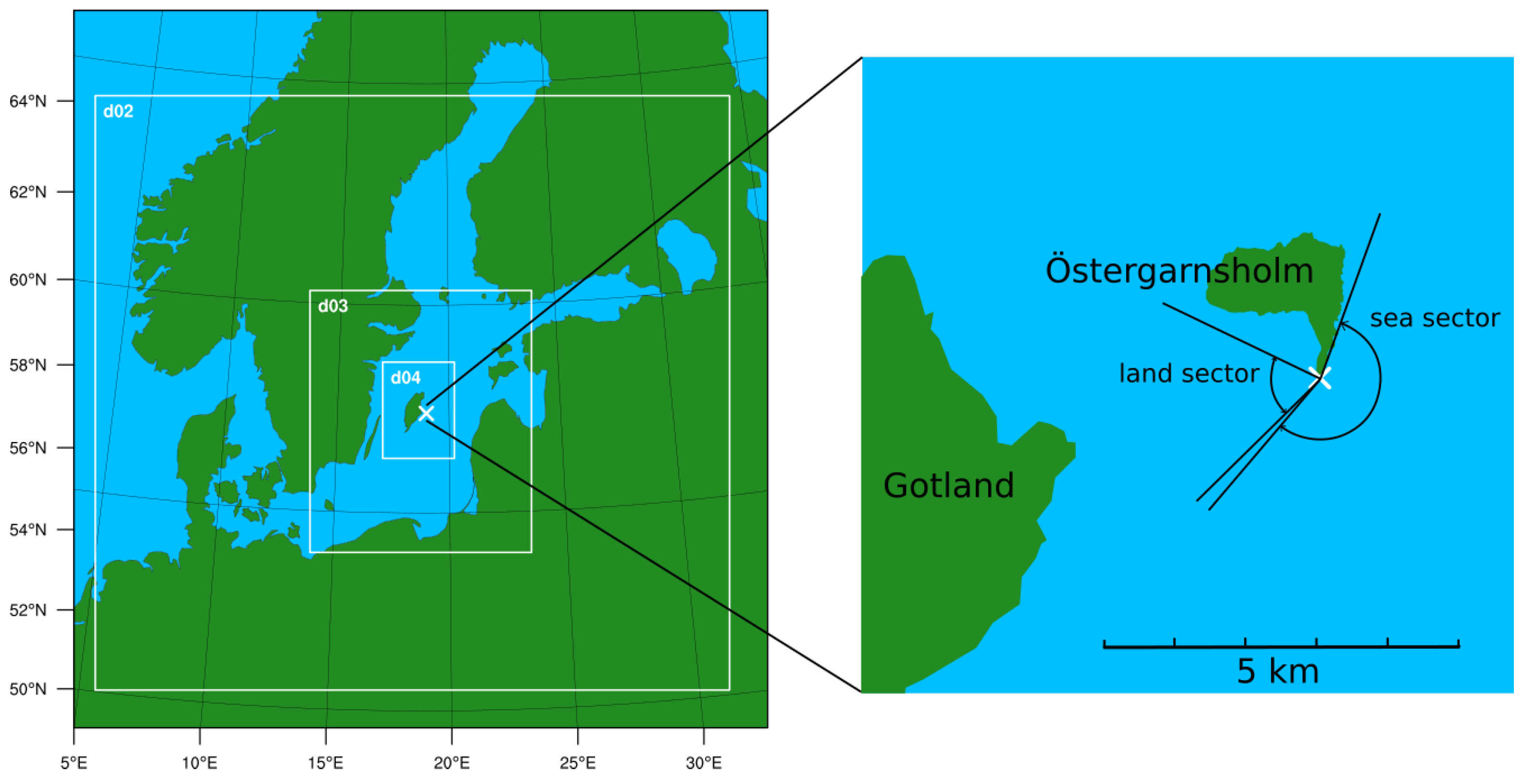
The measurements are performed at the small island Östergarnsholm situated around 4 km east of the larger Gotland island (see
Figure 1) at coordinates 57
25
48.4
N 18
59
02.9
E. The island is flat and without trees, and has a large open-water fetch from several wind directions. A 30 m high meteorological tower is located on the southern tip of the island. Wind speed and direction profiles are measured by Young Wind Monitor propeller anemometers at five heights (7, 12, 14, 20 and 29 m above ground). High-frequency measurements of wind speed and temperature from a CSAT-3D sonic anemometer at 9 and 25 m height is used for calculation of the momentum flux. There is wind speed flow distortion by the tower from directions in the range 355–45
, and these wind directions are taken away in the analyses where the tower data is used. Many air-sea interaction studies have been performed at this site; see Högström et al. [
14] for more detail on the site and instrumentation.
The measurements at the site can be divided into different wind direction sectors depending on the influence of land, sea or a mixture of both. Wind directions from 20–220 are from the sea sector with an open-water fetch of 140 km or more. Wind directions in the range 295–355 are influenced by the land area of the island itself and will not be used in this study. The rest of the wind directions are originating from the land surface of the larger Gotland island with different lengths of over-water fetch. A land sector will be loosely defined as wind directions in the range 225–295. The over-water fetch in this sector after passing the island varies from 4 to 25 km, with the shortest distance from the westerly wind direction.
2.2. LIDAR
2.2.1. Location and Data Collection
A ZephIR 300 LIDAR (ZX Lidars, UK) was placed at the Östergarnsholm field station on 8 December 2016. Data starting from this date and including a full year will be used for this study. The LIDAR is placed approximately 40 m north of the meteorological tower. It measures wind speed (U) and wind direction () profiles, and calculates turbulence intensity () as the ratio of standard deviation, () to the 10-minute average wind speed. The LIDAR can measure at up to ten user defined heights from 10–300 m height, where levels above 200 m are considered an extended range by the manufacturer. It is a 30 conically scanning, continuous-wave LIDAR. It focuses the laser beam at a certain height, thereby retrieving most of the backscatter for that particular height. For each height it makes three revolutions (scans) in the horizontal and then moves to the next level, until all levels are scanned, thereafter it starts again from the lowest height. The measurement frequency of the raw data is 50 Hz, and it takes 1 s to complete one revolution. The wind speed at each height is then averaged over a 10-minute period. The raw data is normally not user-accessible, but this particular unit was modified by ZX Lidars to store the 50 Hz raw data in addition to the standard output. The measurement heights in the present study are chosen to 28, 39, 50, 100, 150, 200, 250, and 300 m above ground surface. Profiles shown will be based on all these heights. The lowest height is approximately equal to the highest level in the meteorological tower, which is at 29 m above ground, because the terrain is slightly sloping upwards to the location of the LIDAR. There are no objects causing distortion of the LIDAR beam, but there is a hut with a height of approximately 2.5 m standing close to the LIDAR. Flow from wind directions of approximately 110–150 pass over the hut before approaching the LIDAR. This can be seen as an increase in turbulence intensity in this wind direction interval compared to the rest of the offshore sector, and therefore these wind directions are not included when analyzing the turbulence intensity.
2.2.2. Momentum Flux Calculations
The LIDAR raw data is used in this study to derive the momentum flux profile. The raw data comes in the form of Doppler-shifted backscatter frequency distributions, , for each of the 50 directions in the horizontal scan. In the case of laminar flow, the distribution becomes very narrow, but the contribution of turbulence within the measurement volume widens the distribution. The width of the distribution is also influenced by velocity gradients within the measurement volume, which is discussed in the section below.
The width of the distribution as function of the scanning direction
(without the influence of velocity gradients) is described by Eberhard et al. [
15].
where
30
is the beam angle to the vertical and
are the (Reynold’s decomposed) fluctuations of the horizontal and vertical components of the wind speed. The radial velocity,
, can be found from the Doppler shift and the wavelength of the LIDAR. In a positive wind speed gradient the correlation of
and
will act to widen the distribution on the upstream side of the LIDAR since negative
and positive
both contribute to lower radial velocity (the velocity along the laser beam), while positive
and negative
both act to increase the radial velocity. On the downstream side, the contributions of
and
will instead counteract each other and hence narrow the distribution. Because of this, the momentum flux,
, can be determined through the difference in distribution width between the upstream and downstream measurements, as in Mann et al. [
16]. In Mann et al. [
16], only the widths in the upstream and downstream directions are used, but in this study we used the full scan, leading to the formula [
15]
To find the width of the distribution of radial velocity, backscatter below a constant threshold are removed to limit the contributions of noise, after which the distribution is scaled to have unit area.
To find 30 min average distributions, , in each of the 50 scanning directions we have used two different strategies, with different advantages and drawbacks. The first method is an arithmetic mean, which has the advantage of retaining all the small-scale variations within the measurement volume. The drawback is that some noise and unwanted backscatter is also retained, which can be a problem for high measurement heights, when the laser is less focused. The second strategy is to identify median velocity within the measurement volume for each 50 Hz distribution and create from those. The drawback of that method is that it filters out small-scale variations, which narrows and makes the actual measurement volume unknown. On the other hand, it has the benefit of being less sensitive to noise contamination. If not otherwise mentioned, the arithmetic mean is used.
To calculate the momentum flux
is fitted to a Gaussian curve, giving
, which is used in Equation (
2). Lastly, the fluxes are smoothed in time using a moving median over 3 h and despiked.
2.2.3. Influence from the Size of the Measurement Volume
Since the LIDAR is of the continuous-wave type, the length of the measurement volume (in the direction of the beam) increases quadratically with distance due to better focus at short distances. Actual backscatter depends on the focus of the beam, the amount of backscatter particles in any given volume and attenuation of the laser beam. If the distribution of particles is homogeneous and the attenuation is negligible, the shape of the measurement volume is described by a Lorentz distribution of the Rayleigh length [
16]. A property of the Lorentz distribution is that it has infinitely long tails, and hence the total length of the measurement volume is strictly speaking infinite as well. However, the distribution has a distinct peak, and 50% of the volume lies within
vertical m at 28 m height, compared to ±80 vertical m at 300 m height. The radius of the scanning circle also increases with distance, and is 16 m at 28 m height, compared to 173 m at 300 m height. The measurement volume thus represents a considerable filter for
making
and
measurements uncertain at higher heights.
As mentioned above, vertical velocity gradients within the measurement volume will lead to a widening of , and thus an increase of . However, the calculation of momentum flux is done by the means of difference between opposite sides of the scan and hence the effect of a widened distribution due to velocity gradient is cancelled out and the flux is simply a weighted average of the flux within the volume.
3. Model Setup
In this study, the ARW WRF (Advanced Research WRF) model version 3.8.1 is used. Simulations are performed for the period 8 December 2016–7 December 2017. The model area is centered on the Östergarnsholm site, and consist of four domains with resolutions of 27, 9, 3, and 1 km respectively in both horizontal directions.
Figure 1 left shows the placement of the three inner domains. The analysis is based on data from the innermost domain. There are 48 vertical levels, with an increased resolution close to the surface to capture boundary-layer processes; for example, there are 12 levels below 100 m. The model is restarted every day at 12 UTC, and the first 12 h are used as spin-up time, because studies have shown that it takes a long time for the surface fields to reach equilibrium [
17]. The input data is from ERA-Interim with 0.75
horizontal resolution, which has been shown to give good results compared to other reanalyses [
17,
18]. The input data is fed to the WRF model boundaries every 6 h.
The different physics packages used in the simulations are the Noah land-surface scheme [
19], MYNN2 boundary-layer scheme [
20], MYNN surface layer scheme, RRTM longwave radiation scheme [
21], Dudhia shortwave radiation scheme [
22], Thompson microphysics scheme [
23] and the Grell 3D cumulus physics scheme [
24,
25]. The cumulus physics is applied only on the two outermost domains.
The boundary-layer wind speed in WRF is calculated by a surface layer and a boundary-layer scheme. In the surface layer scheme surface values (2 m temperature and mixing ratio and 10 m winds) and surface fluxes (if over ocean) are calculated. In the boundary-layer scheme fluxes of momentum, temperature and moisture are distributed vertically, and entrainment is taken into account. The boundary-layer parameterization is based on the assumption that sub-grid scale turbulence is not resolved, and therefore can be parameterized. The MYNN2 boundary-layer scheme is based on 1.5 order closure, where the turbulent fluxes are a function of turbulent kinetic energy.
4. Theory
Simulations during non-neutral stratification have been shown to deviate more from observations compared to neutral [
26,
27]. Especially stable conditions and LLJs are hard to capture, and therefore the focus of this paper will be on these conditions. There are several creation mechanisms of LLJs over the sea surface. They can be created along coastlines due to the land-sea temperature contrasts and the associated baroclinicity [
28]. In cases with low synoptic wind speeds sea breeze circulations can occur, creating a LLJ at low height with onshore winds. During the day the wind direction may be affected by the Coriolis force, and become more coast-parallel. A third important mechanism of LLJ formation over the sea surface is creation by inertial oscillations, when the wind is coming from a heated land surface out over the colder sea surface. When the friction created by the convection is suddenly shut off at the coastline, inertial oscillations can cause the wind speed to accelerate in the stable boundary layer [
29].
There are several ways to define a LLJ. For the identification of LLJs in this study four different classification criteria are used:
- (1)
A wind speed being 1 m s stronger than the wind speed at any of the abovelying levels of the LIDAR wind speed profile. Often a criterion of 2 m s exceedance is used, but it is probable that many jets would be missed with a stricter criterion because of the limited height range of 300 m.
- (2)
A wind speed being 1 m s stronger than the wind speed at any of the abovelying levels up to 300 m height, based on the WRF model wind speed profile. This is the same criterion as is used for the LIDAR (crit. 1).
- (3)
A wind speed being 2 m s stronger than the wind speed at any of the abovelying levels up to 1000 m height, but with a jet core at or below 300 m height, based on the WRF model wind speed profile. With this criterion possibly more LLJ cases can be included due to the information from higher heights, but the results are still comparable to crit. 1, because of the restriction of the jet core height.
- (4)
A LLJ occurring simultaneously in both the LIDAR and WRF wind speed profile, based on crit. 1 and 2.
The LLJ should be persistent for at least three consecutive hours in all classifications.
To be able to compare turbulent quantities between the LIDAR and WRF the turbulence intensity (
) from WRF is calculated from turbulent kinetic energy through the relation
where
e is the turbulent kinetic energy and
U the wind speed, for wind speeds
. This is an approximation, and may not give a completely realistic representation of the turbulence intensity. It is used to compare the shape of profiles of
from the LIDAR and WRF, and not for comparison of the exact magnitude.
The momentum flux,
, from the WRF model is calculated according to
where
is the eddy diffusivity from the model and
is the wind speed gradient across the two nearest model levels from the same time step.
5. Results
5.1. Comparison of Tower and LIDAR Data
5.1.1. Wind Speed and Direction
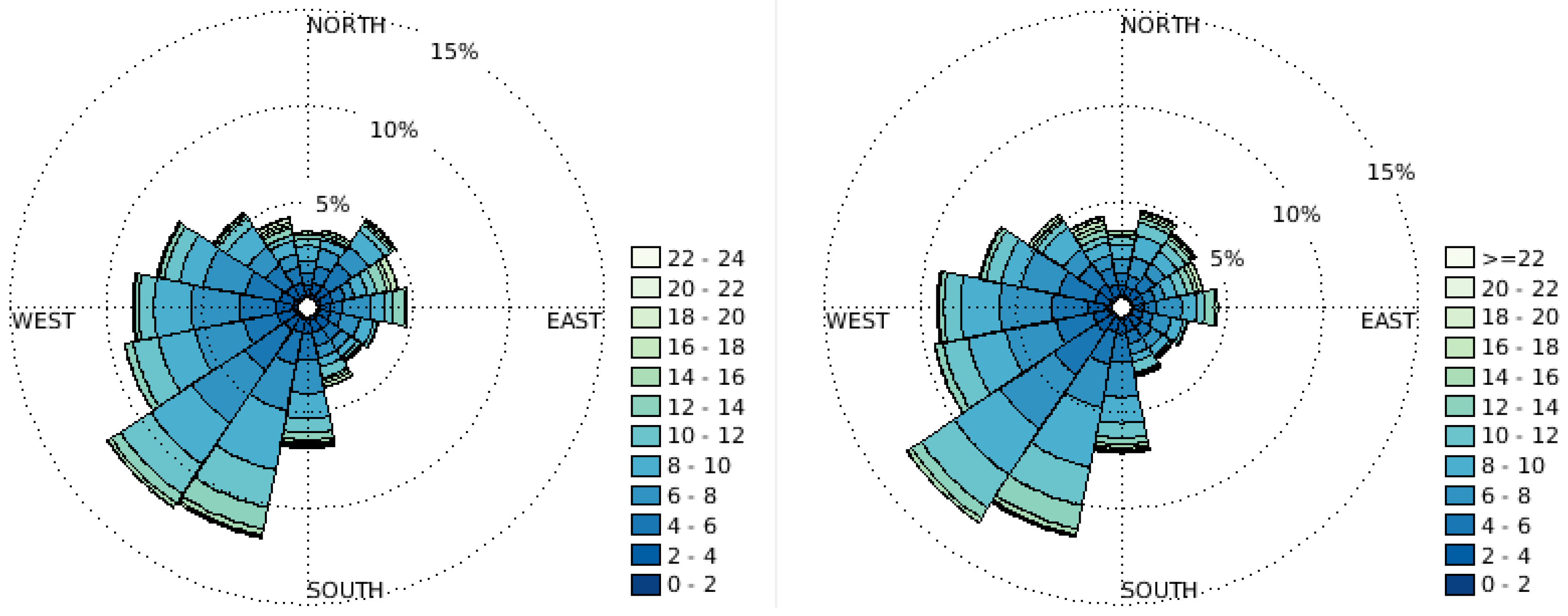
The data availability for LIDAR profiles is 92% during the year of interest and 85% for tower wind speed profiles. Windroses from the propeller anemometer and the LIDAR at 29 and 28 m height respectively are shown in
Figure 2. Please note that also the wind directions in the range 355–45
are included in this plot, although the tower data is subject to wind speed distortion in this sector. The wind direction is generally southwesterly, but with westerly wind directions also being common. The agreement is good between the two types of measurements, and only small differences can be seen.
In
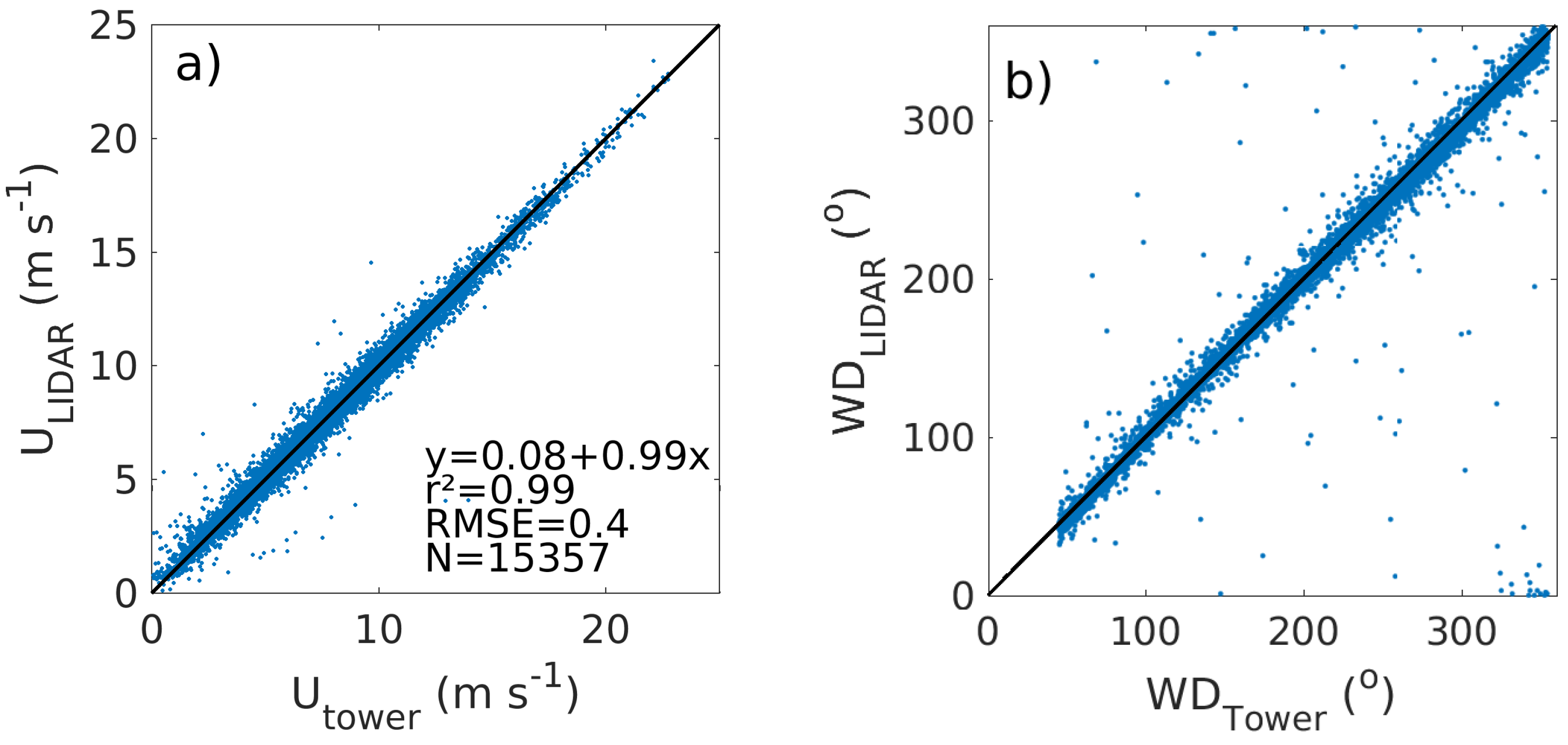
Figure 3 scatter plots of half-hourly averaged data from the propeller anemometer and LIDAR at 29/28 m height are shown. Only sectors where the instrument on the tower is not obstructed are included. There is good agreement and a high correlation with
and RMSE = 0.4 for wind speed. For wind direction most of the data is gathered around the 1:1 line, but there is some scatter, most of which occurs at low wind speeds, and is not unexpected. There are also a few instances when the LIDAR gives the incorrect, shifted by ±180
, wind direction. This is because the LIDAR is homodyne, i.e., the sign of the Doppler-shifted return signal cannot be distinguished. The wind direction is instead determined by choosing the direction of one of the two wind speed maxima along the scanning circle which is closest to the wind direction measured by a weather station at the LIDAR unit. Based on the tower measurements, these data points (1.7% of the total data), are shifted by 180
and can therefore not be seen in the figure. In general, the good agreement between the tower and the LIDAR makes it possible to use the LIDAR for evaluation of the WRF model when it comes to first order average quantities.
5.1.2. Turbulent Quantities
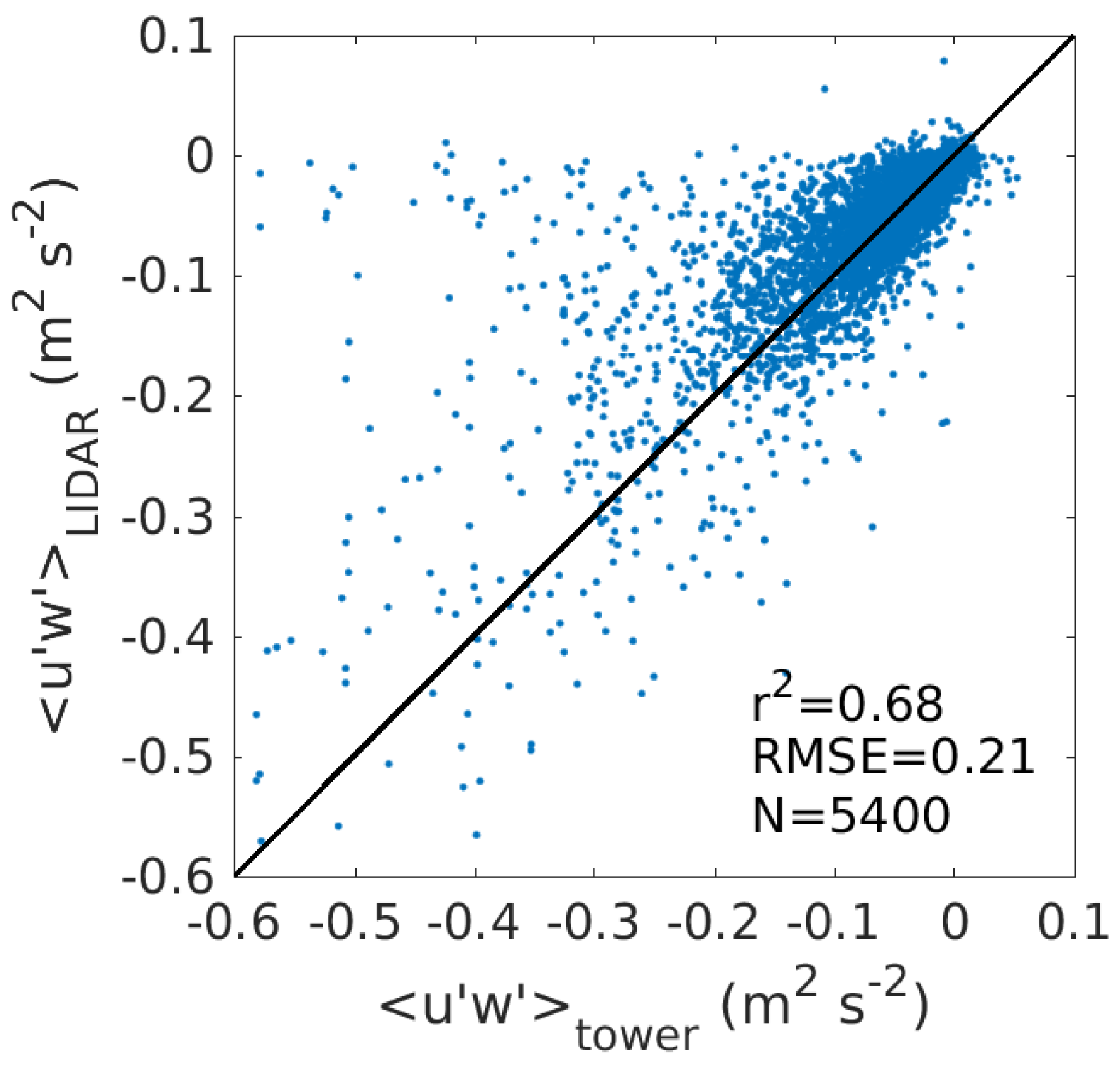
Figure 4 and
Figure 5 show a scatter plot and a time series of momentum flux calculated from the sonic anemometer at 25 m height and the LIDAR at 28 m height. The scatter data is from the period 18 April–30 November 2017, when tower data is available. The time series is from the month of May, a period during which LLJs are common, and therefore will be the focus for this paper. There is large scatter in the data (
= 0.68 and RMSE = 0.21), but from the time series in
Figure 5 a clear relationship is observed between the two data sets. Comparing with the longer time period available from the anemometer at 10 m height gives
= 0.56. The scatter appears due to uncertainties in the magnitude of the fluxes, whereas the timing of high/low flux events is good.
5.2. Comparison of LIDAR and WRF Data
5.2.1. Wind Speed and Direction
Profiles of wind speed and turbulence from LIDAR and WRF are shown in this section, as well as a comparison at 100 m height. The 100 m height is chosen because this is close to the typical hub height of offshore wind turbines, and because we expect a larger influence of mesoscale effects at this height, and it is important to evaluate how well the model can capture these.
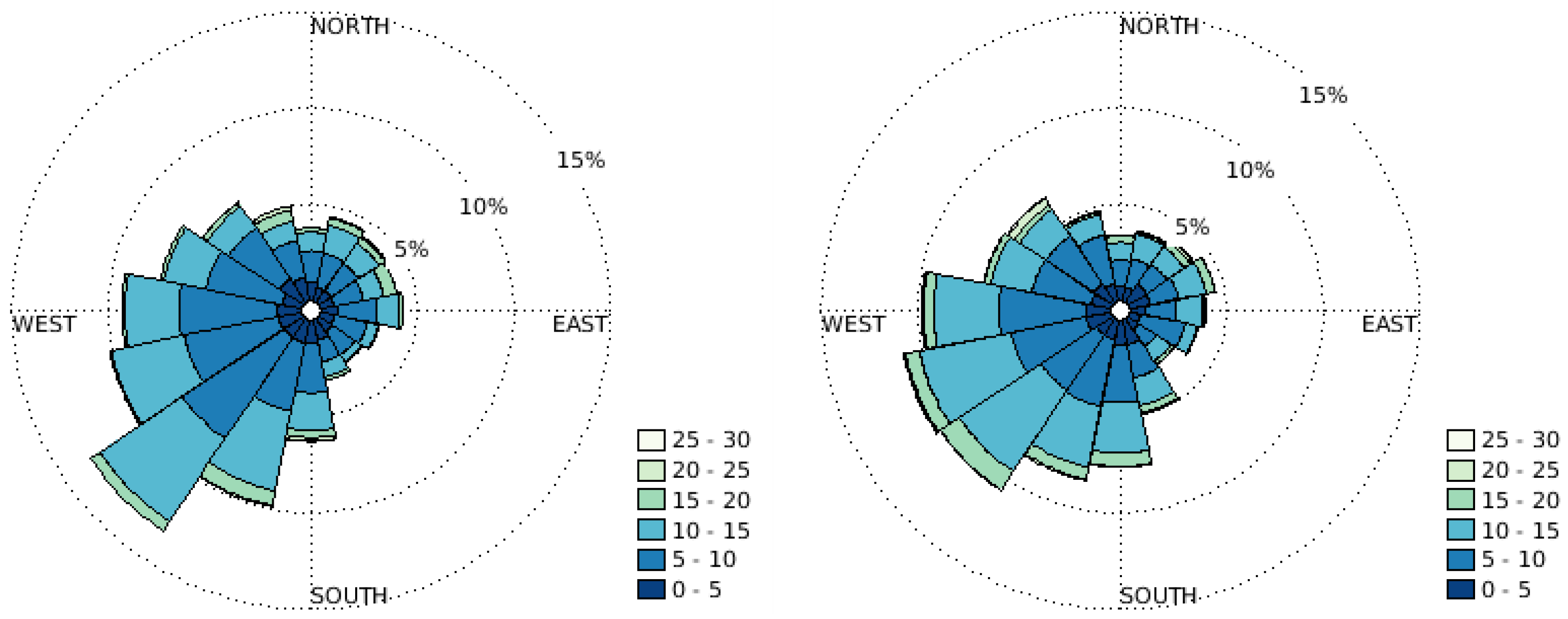
Figure 6 shows the windroses from LIDAR and WRF at 100 m height. The wind direction in the WRF model is shifted towards more west-southwesterly and westerly winds compared to the LIDAR, where southwesterly winds are more common. This is possibly implying an underestimated roughness over the Gotland island, which would make it possible for the winds to pass Gotland to a larger degree instead of following the coastline. Also, southerly winds are more common in the model simulations. Winds are coming from the sea sector in 37% of the cases.
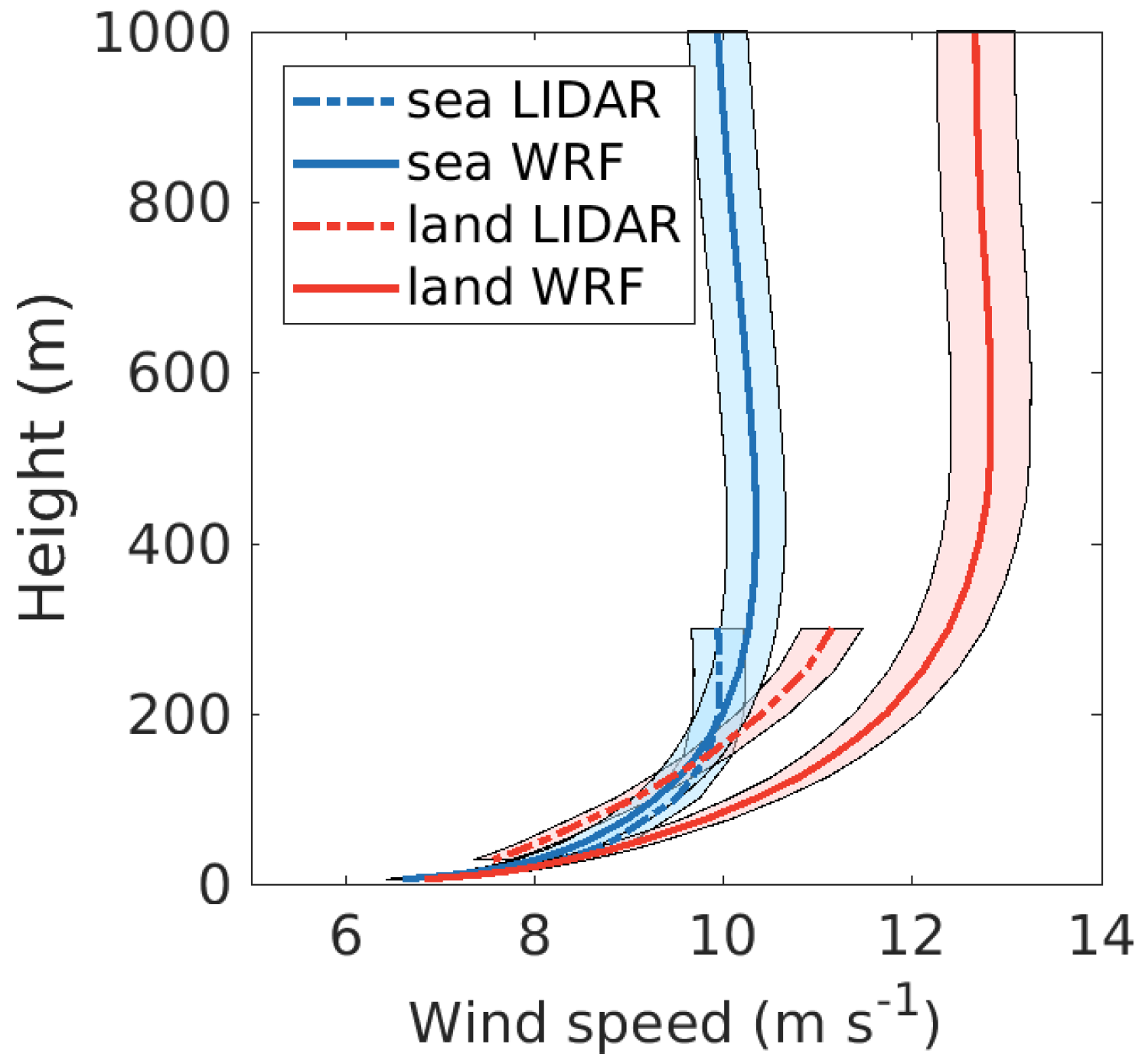
Figure 7 shows the mean wind speed profiles divided into sea and land sectors. The filled contours in this and the following figures show the standard deviation of the mean,
, where
is the standard deviation and
n is the number of independent data points, assumed to be every 11th hourly data point in the case of wind speed, every second data point in the case of turbulent quantities and every 3rd hourly data point in the case of wind speed profiles created from cases with LLJ occurrence. In the directions with long open-water fetch there is a close agreement between the measured and modelled wind profiles up to 250 m height, while for the wind directions coming from the main island, there is an overestimation of the wind speed for all heights. As mentioned above, this may be due to an underestimated roughness length over the land surface of the Gotland island. Similar results in this respect were found by Hahmann et al. [
30] in their WRF evaluation against the meteorological tower at the same site. Since the focus of this study is on offshore conditions, it will not be studied in more detail.
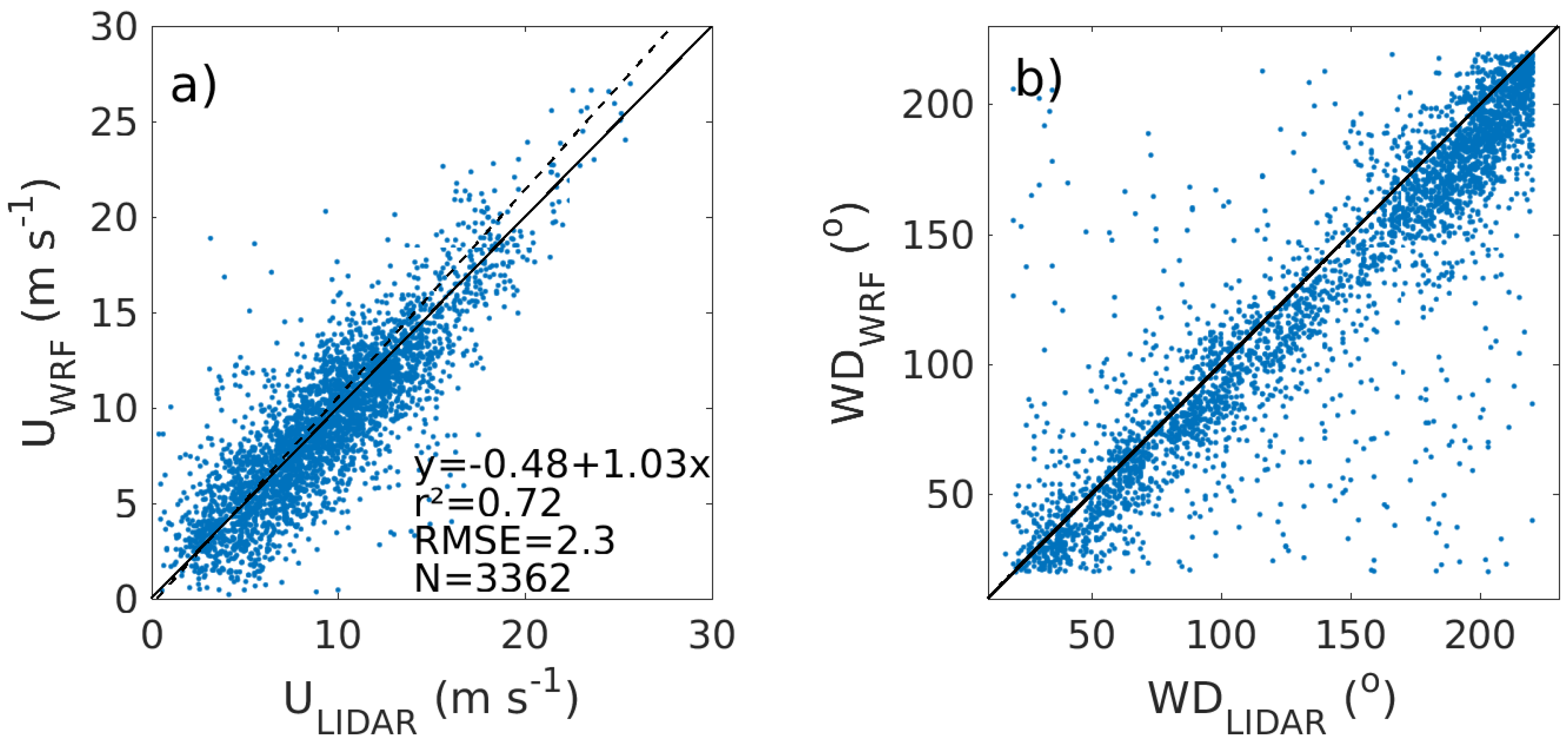
Figure 8 shows scatter plots comparing data from LIDAR and WRF at 100 m height with wind directions from the sea sector. Corrections are made for LIDAR wind directions differing with 180 ± 20
from the simultaneous tower data. There is larger scatter and lower correlation (
= 0.72 and RMSE = 2.3) than for the tower-LIDAR comparison. In this case, the wind direction scatter is not only occurring during low wind speeds. The regression line suggests that there is a slight overestimation of the wind speed in the WRF model. The correlation does not vary markedly with height.
Table 1 shows the variation of the bias and root mean square error with season. The bias generally approaches zero or becomes positive at higher height, whereas it is negative at lower heights. This shift is most notable during spring and summer, when the bias has maximum positive values at 200 and 300 m height. The root-mean-square error is smallest in winter compared to the other seasons, and similarly the correlation is high in winter (not shown). At 300 m height the root-mean-square error becomes larger in spring and summer.
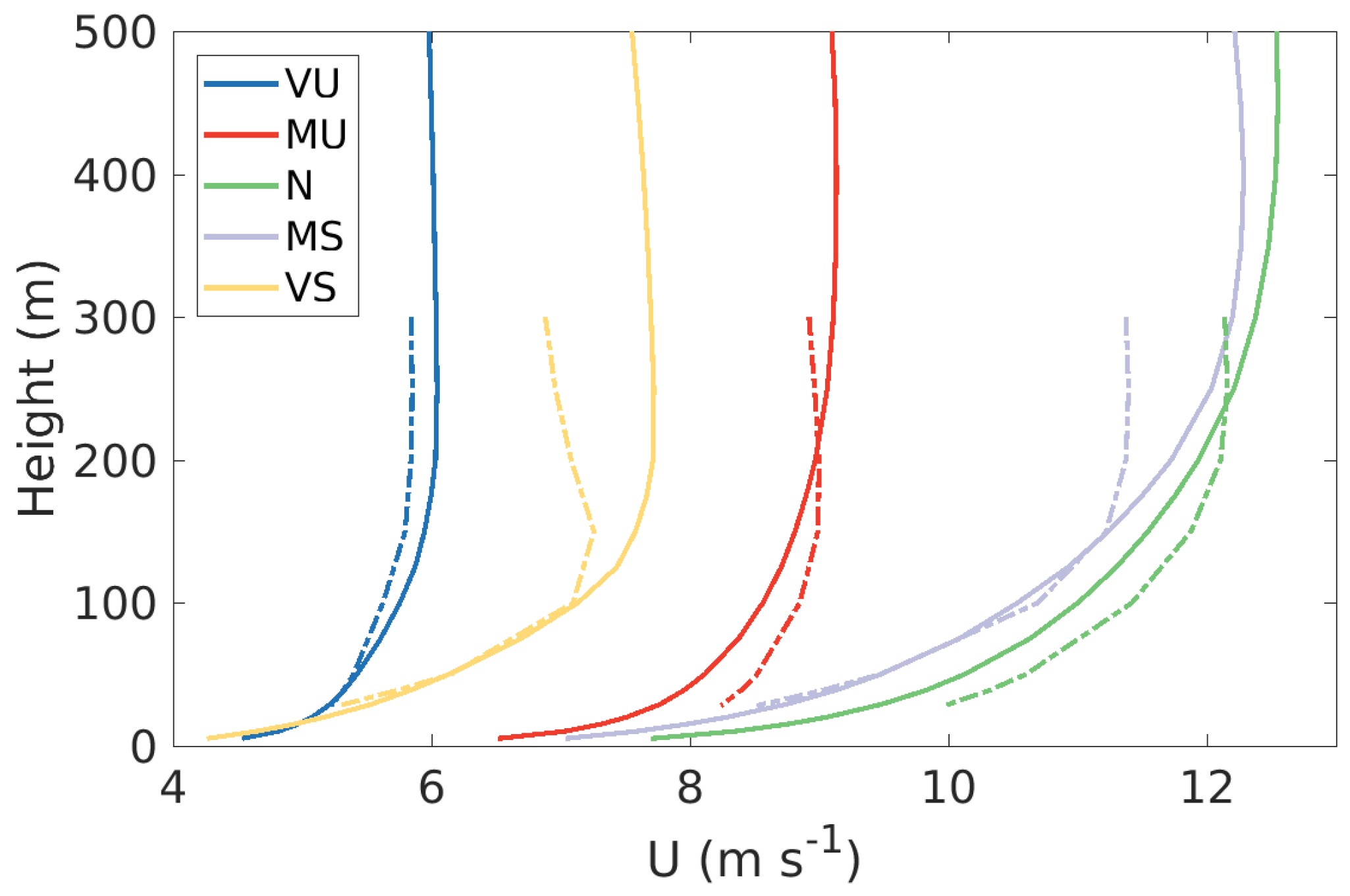
Figure 9 shows mean wind speed profiles from the sea sector divided into different stability categories. As expected, the wind speed is highest for neutral conditions, but also high for moderately stable conditions, indicating that there are many close to neutral cases in this class. The wind speed is lowest in the very unstable and very stable classes, and it is likely the occurrence of LLJs that is responsible for the higher wind speed in the very stable class compared to the very unstable. It can be see that there is a positive wind speed bias in the WRF model during moderately to very stable conditions. Very stable conditions occur mostly during May and June according to the tower measurements, and LLJs are common. In the average wind speed profile during very stable conditions a climatological LLJ can clearly be seen in the measurements, but not in WRF. The WRF overestimation is mostly occurring at high heights, which can also be seen from the yearly variation of the errors (
Table 1).
Table 2 shows the bias and root-mean-square error at 4 heights divided into the same stability classes. The bias is clearly largest for moderately and very stable conditions at 200 and 300 m height, although the root-mean-square error is largest for neutral conditions at most heights. However, the highest wind speeds also occur in this class, which increases the error. The root-mean-square error normalized by the average wind speed is in almost every case largest for very unstable and very stable conditions.
5.2.2. Turbulent Quantities
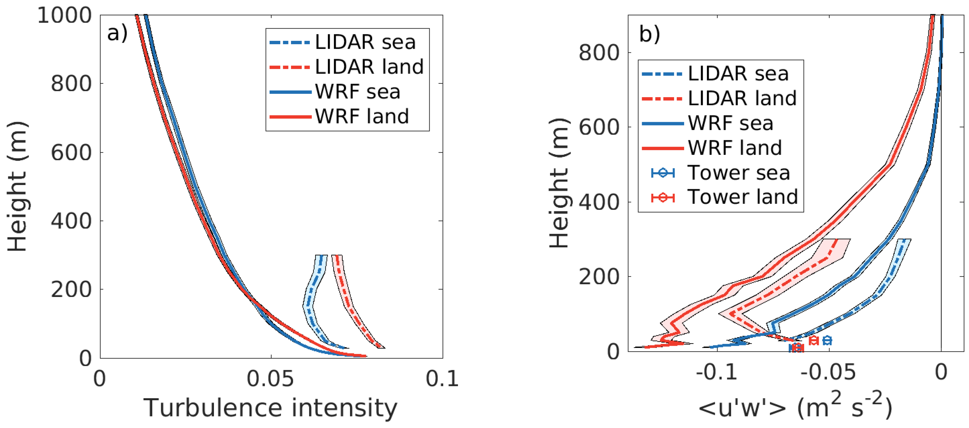
Figure 10 shows the mean profiles of turbulence intensity and momentum flux from LIDAR and WRF data divided into sea and land sectors. The WRF profiles of turbulence intensity from the land and sea sectors are of similar magnitude and shape, decreasing rapidly with height, whereas the LIDAR data decreases slowly or increases with height. Systematic errors of the LIDAR due to averaging over the large sampling volume at higher heights is expected to underestimate the wind speed standard deviation compared to measurements with a sonic anemometer [
31]. In this case, we do not see signs of underestimation, but possibly an overestimation. A similar trend can be seen in Mohr et al. [
32], which reported an overestimation of
at 173 m height, using the same type of instrument, while values up to 100 m agreed with tower measurements. Therefore we cannot conclude that the turbulence intensity measurements at heights above 150 m are correct. The increasing
with height over sea is an indication that shear-induced turbulence created by LLJs can create this profile shape, but the differences between the land and sea profile could also partly depend on systematic differences in atmospheric stability or vertical distribution of scattering particles.
Figure 10b shows the mean momentum flux profiles from both sectors. Momentum fluxes originating from the land surface are higher than the fluxes originating from the sea in both simulations and observations, implying advected turbulence from the land surface. In the lowest 75 m of the WRF profile from the land sector fluxes are close to constant with height, implying that there is an internal boundary layer approximately up to this height. A similar behavior can also clearly be seen in the LIDAR profile originating from the land sector. Up to 100 m height the magnitude of the flux increases with height, above which it starts decreasing again, likely implying an internal boundary layer created by the advection from the land surface. The shape of the momentum flux profiles is relatively similar in the measurements and simulations, although the magnitude is higher in WRF. The momentum flux from the WRF model is parameterized as a function of wind shear, turbulent kinetic energy and stability, and does not necessarily need to have the same magnitude as the observations. Compared to the tower measurements the magnitude of the LIDAR data is higher, as a result of higher peak values, something which can also be seen in
Figure 5.
5.3. Low-Level Jet Occurrence
Low level jets have the potential to modify mean wind and turbulence conditions considerably. In this section, statistics of LLJ occurrence and evaluation of the WRF model during LLJ occurrence is presented.
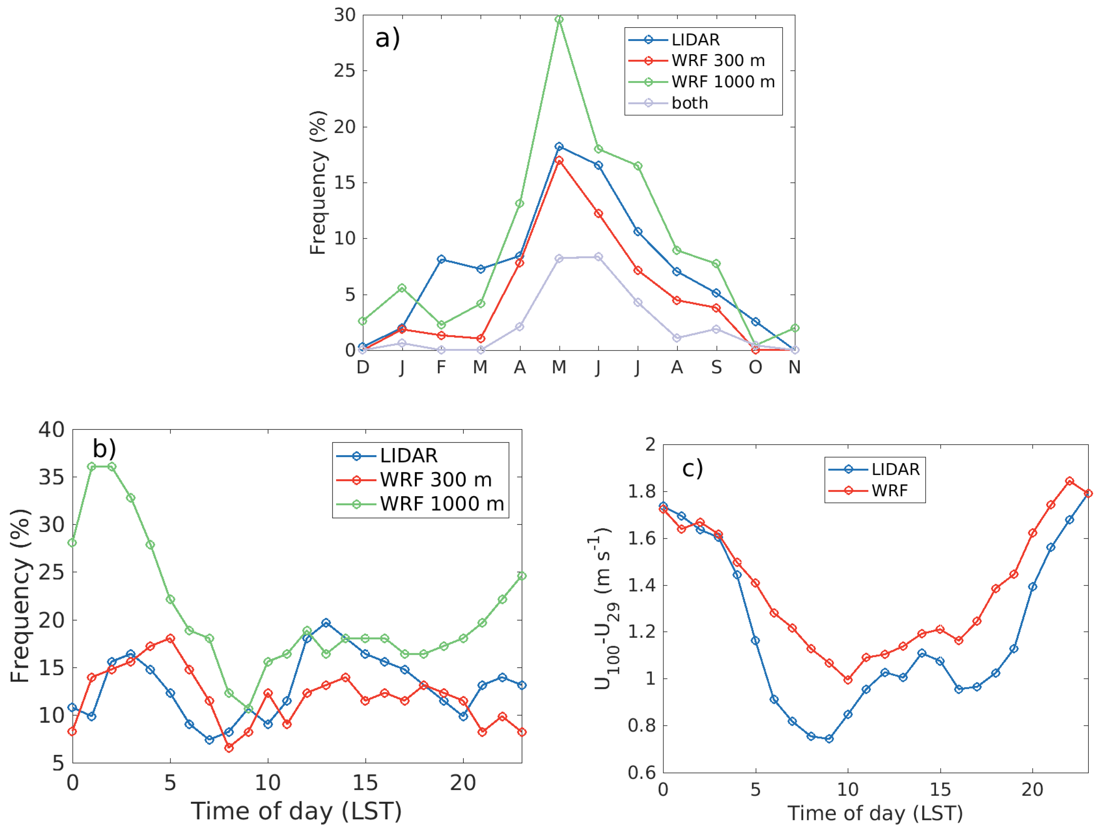
Figure 11a shows the frequency of LLJ occurrence each month classified in four different ways. From the classification made from the LIDAR data (
crit 1 introduced in
Section 4) it can be seen that LLJs are most common during May (occurring 18% of the time in the LIDAR data), and thereafter June (17%), when there is also a large frequency of stable conditions [
7]. If the classification is relaxed so that the LLJ does not have to be persistent for at least three hours, the frequency increases to 27% in May and 25% in June.
From the simulation results it is clear that there is always more jets if using data up to 1000 m height (crit. 3), compared to using data up to 300 m height (crit. 2). Especially in May, the differences are very large, showing that the simulated LLJs commonly occur either with their jet core close to 300 m height, or with a slow wind speed decrease with height above the jet core. When using the same classification for both data sets (crit. 1 and crit. 2), the number of LLJs is fairly similar, but with higher frequency in the LIDAR data. However, when only choosing LLJs which are coexisting in both LIDAR and WRF data, the frequency decreases. In May this effect is most pronounced, in which case the frequency is approximately halved compared to the observed number.
Figure 11b shows the diurnal variations of LLJ occurrence. From the WRF data up to 1000 m height (
crit. 3) it can be seen that LLJs are most common during the nighttime. Similar results can be seen in Svensson et al. [
7]. These LLJs are likely often created by warm-air advection initiated during the previous day or by LLJs advected from the mainland, created due to nighttime cooling over the land surface. According to the WRF simulations LLJs often cover the whole sea surface of the inner model domain at this time of day, showing that it is likely not a local phenomenon creating these jets. According to the tower data the frequency of stable stratification is also largest during nighttime (not shown).
Figure 11c shows that the average wind shear is largest during the nighttime in both simulations and observations. Since an increased wind shear is connected to LLJ occurrence, this indicates that LLJs are common during the nighttime also in the LIDAR data, but that these jets have too high peak heights to be classified as LLJs.
There is also a peak in occurrence during the middle of the day, most clearly seen in the LIDAR data (
Figure 11b). This suggests that sea breezes or coastal jets form during this part of the day due to the temperature contrast between the Gotland island and the sea surface. A larger fraction of the LLJs have along-coastal wind direction during this time of day compared to the nighttime jets. However, according to the model simulations, there are only a few cases of pure coastal jets, and most LLJs cover large areas over the sea surface. This indicates that small-scale, local LLJs may be hard to capture in the model.
The number of days with LLJ occurrence during at least three consecutive hours varies from 0 in November to 18 in June. Low level jets occur with winds from all wind directions, but are most common for offshore winds. The largest percentage of LLJs occur for southeasterly wind directions.
5.4. LLJ Characteristics
Figure 12 shows the mean wind speed profiles during LLJ occurrence. In
Figure 12a the classification is made from the LIDAR data (
crit 1), in
Figure 12b from WRF data below 1000 m height (
crit 3) and in
Figure 12c the LLJ has to exist in both classifications (
crit 4). It can be seen that although both data sets exhibit LLJ wind profiles they do not always occur simultaneously or have the same characteristics. The average LLJ classified from the LIDAR data has a jet core at 100 m height and a maximum wind speed of 7.8 m s
(
Figure 12a). This is in sharp contrast to the simultaneous WRF wind speed profile, which only show a slight tendency for a LLJ. In many cases, this occurs in connection with a strong change in wind speed, which means there is a difference in timing between the LIDAR and WRF data. In many cases, there is a LLJ in both data sets, but it is less extended in the vertical in LIDAR data. It also happens in a few cases that there is a LLJ in the LIDAR which is not present at all in the WRF data. These jets usually occur during low ambient wind speed, and do not extend to high heights.
The average LLJ classified from WRF below 1000 m has a wind speed of 8.7 m s
at 200 m height, with the wind speed in the simultaneous WRF profile 0.9 m s
stronger (
Figure 12b). During simultaneous cases (
Figure 12c) there is substantially fewer values. The agreement between model and measurements is good below the jet core, and relatively good above the jet core, where the WRF profile decreases a little less rapidly with height compared to the LIDAR data. The jet core height and strength is well captured.
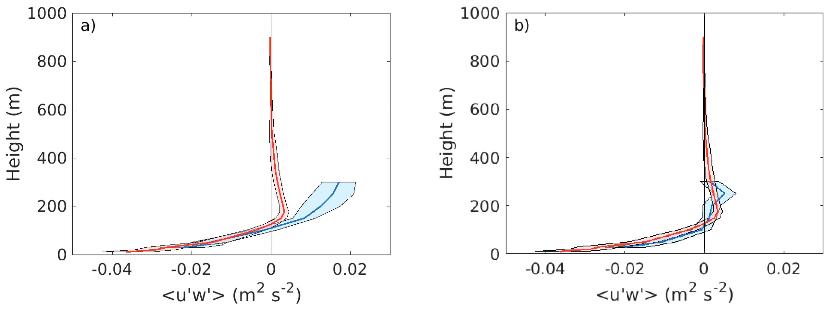
Figure 13 shows the mean momentum flux profiles during LLJ occurrence calculated using two different methods to estimate
, see
Section 2.2.2. Both methods agree with each other and with the WRF data below 150 m height, but give different values above the jet core. Both model and observations show a positive momentum flux above 125–150 m height, but the maximum magnitude and the profile shape varies depending on which method is used. In
Figure 13a the flux is determined from
calculated by arithmetic mean, thus ideally giving a full representation of the weighted average flux in the measurement volume. The large positive values could however be an artifact of a heterogeneous distribution of scattering particles within the measurement volume.
Figure 13b shows flux estimates from
estimated by filtered
measurements, which omits flux contributions from small-scale turbulence, but is less sensitive to measurement error. Here, a peak flux is seen at 150 m height, indicating that this may be a truer profile shape compared to the one calculated by the arithmetic mean, and it agrees reasonably with the WRF data. As the size of the scanning volume increases strongly with height, each of the upper heights are likely influenced by the surrounding heights, creating an additional uncertainty of the flux estimation.
5.5. Example of LLJ Cases
In this section, examples of LLJ cases from May and June will be shown.
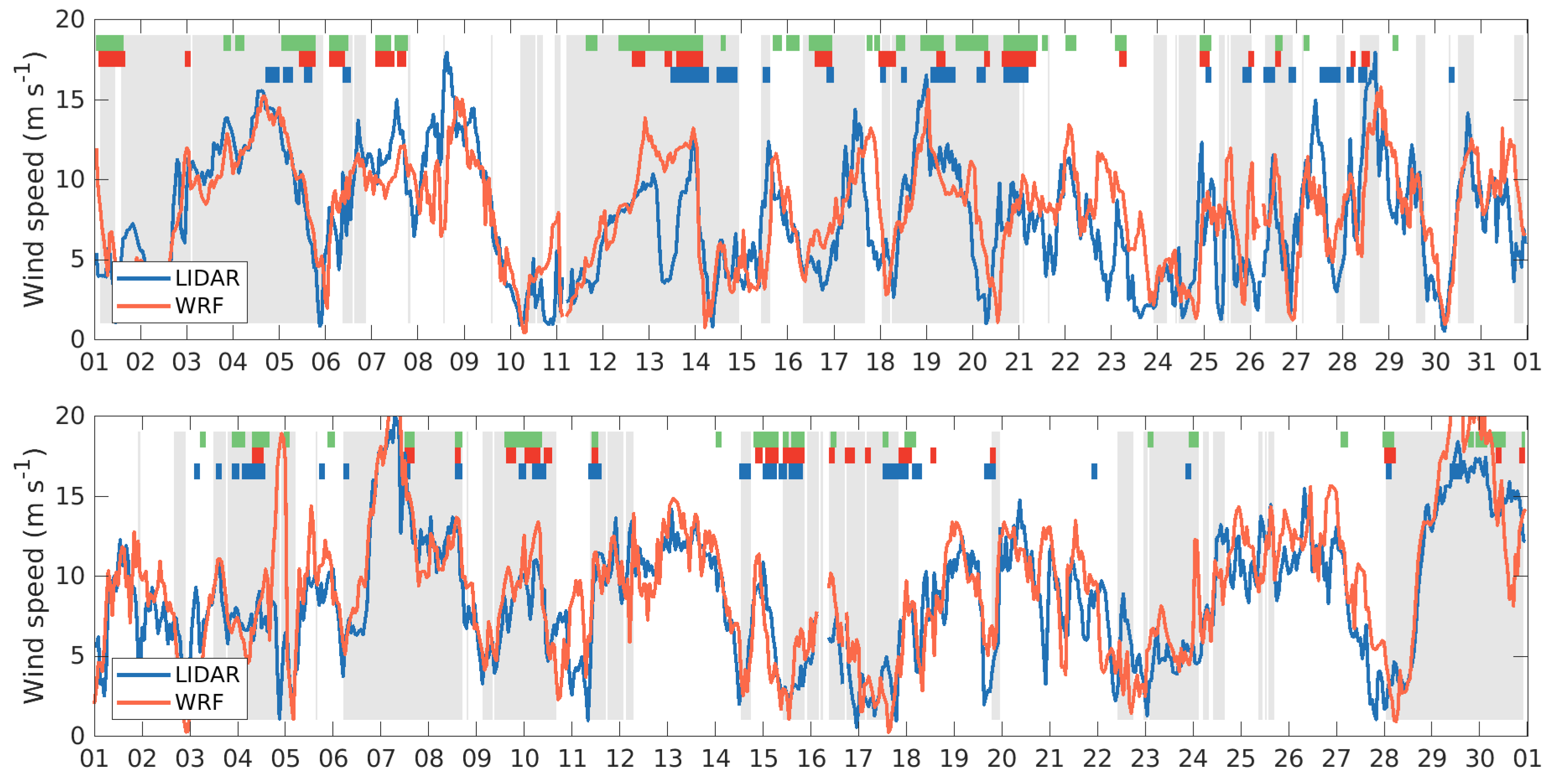
Figure 14 shows the wind speed at 100 m height from the LIDAR and WRF during May and June 2017. The filled areas in the upper part of the figure show occasions with LLJ occurrence, classified in three ways as described in
Section 4. It is clear that there are several occasions with no overlap between the events from different classifications, and numerous cases where the events are of different lengths. When the classification is made including heights up to 1000 m (green color) it can be seen that LLJs are frequent and long-lasting. Nonetheless, there are events captured by the LIDAR which are not visible in WRF even with this larger height range. It can be seen that the wind speed sometimes increases substantially during LLJ occurrence (e.g., 12–13 May, 18–19 May, and 6–7 June), but sometimes LLJs occur also during lower wind speed (e.g., 14 May). The wind speed correlation does not seem to be markedly lower with LLJ occurrence than without.
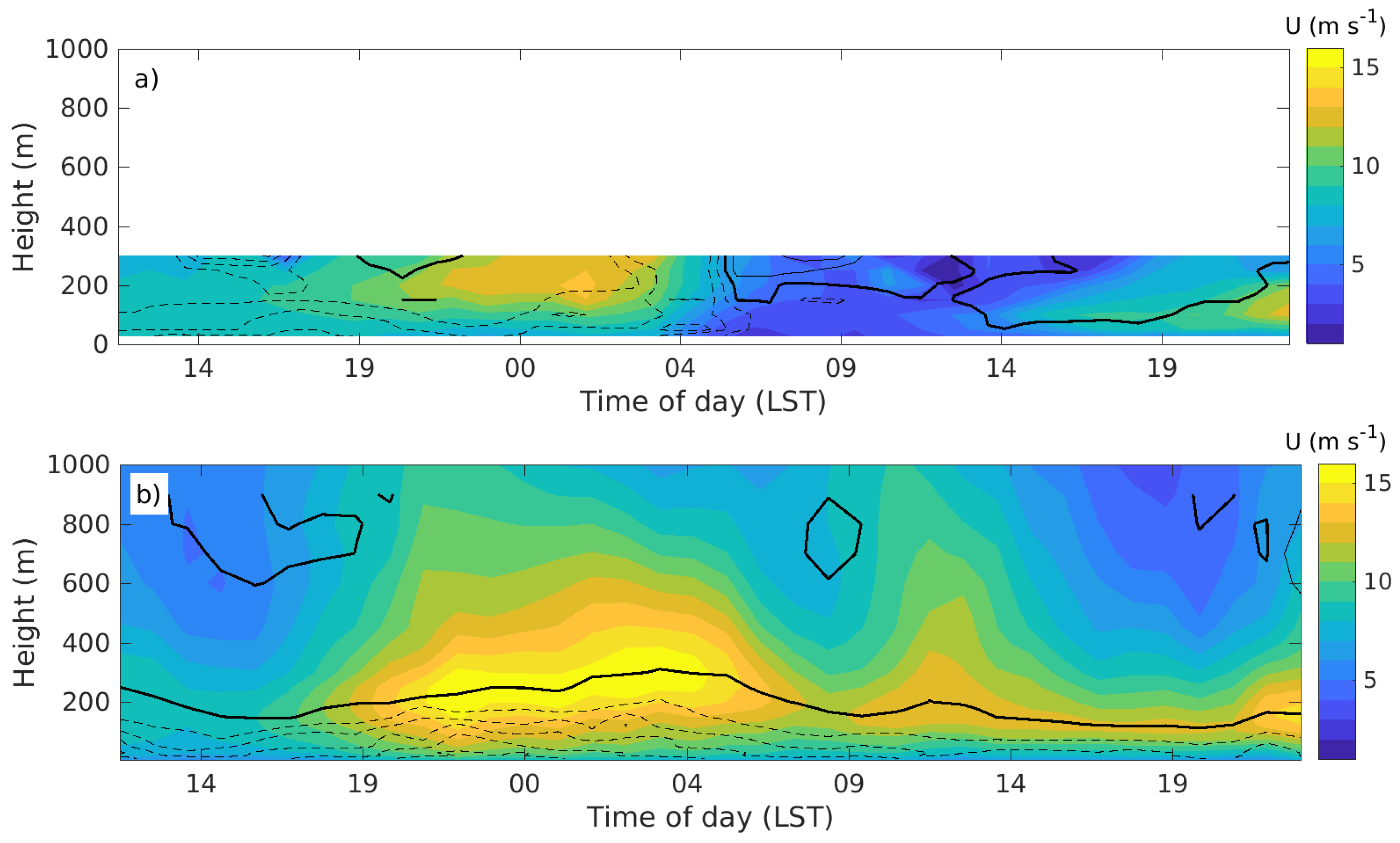
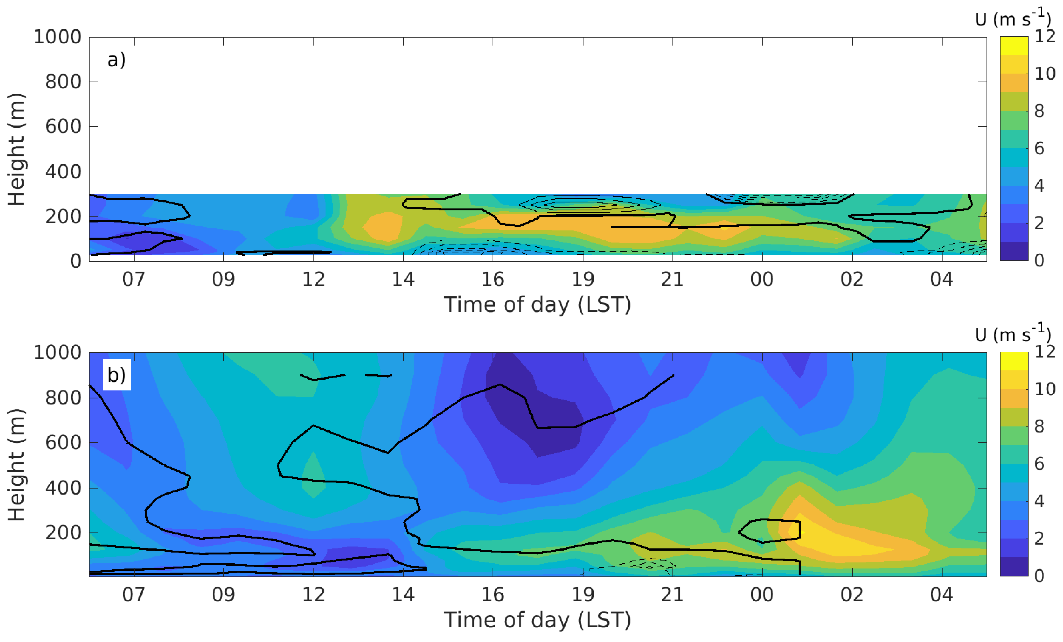
Figure 15 and
Figure 16 shows examples of time-height cross sections of wind speed from the LIDAR and WRF during two occasions with winds predominantly from the sea sector. Here it can be seen that there are significant differences in the LLJ portrayal in the measurements and simulations, showing that for specific cases simulations are still uncertain and cannot capture all the wind variability.
On 12 May (
Figure 15) a LLJ is created around 15 LST (Local Standard Time), and is persistent for the whole evening and part of the following day. According to model simulations it is covering almost the entire southern Baltic Sea. The wind direction is easterly and brings warm air from the Baltic states out over the sea surface. The LLJ is also seen in the sounding from Visby airport (not shown) on the Gotland island at 00 UTC and faintly at 12 UTC. The difference between simulations and observations during midday on 13 May are explained by diverging atmospheric conditions. The measurements from both the tower and the LIDAR show that the wind speed decreases with ∼6 m s
during the middle of the day, and at the same time the temperature drops with ∼4
C and the stratification becomes unstable. This momentary situation of unstable stratification is not captured by the model, which explains the difference in wind speed.
The momentum flux in the LIDAR data is in general positive above the jet core and negative below with large variations in time. The momentum flux in WRF shows similar behavior, but with less variations in time. The flux is by definition positive above the jet core because of the negative wind speed gradient.
On 20–21 May (
Figure 16) there is a strong LLJ in both LIDAR and WRF data during the second half of the day and the following night, but with the wind speed maximum limited to lower heights in the LIDAR than in WRF. The wind turns from southerly to easterly during the day, and the likely creation mechanism is once again warm-air advection. The momentum flux from the LIDAR again varies considerably in time, but being positive close above the jet core. The momentum flux in WRF is close to zero above the jet core, and thus shown no positive peak above the jet.
As can be seen there are several ways in which the portrayal of LLJs in the observations and simulations may differ. It can be in height, timing or that a LLJ exists in one of the data sets but not the other. The reason for this can be either problems with the input data or the model parametrizations, which can give rise to differences in timing, location or characteristics of LLJs.
6. Discussion and Conclusions
Wind and momentum flux profiles from a continuous-wave LIDAR and the WRF model at an offshore site are analyzed to present wind characteristics in the marine environment. Firstly, LIDAR data is evaluated against tower measurements, and the good agreement between the tower and LIDAR wind speed and direction measurements makes it possible to use the LIDAR for evaluation of the WRF model.
Comparing the wind speed from the WRF model against the LIDAR shows a general scatter of a few meters per second, and there is a positive bias from wind directions originating from the land surface at all heights. The main focus is on the offshore conditions, where differing atmospheric conditions influence the wind speed errors from 200 m height and above. The largest bias occurs for stable conditions, where it is ∼0.8 m s at 300 m height. The bias is generally positive and large during spring and summer and during stable conditions at these heights.
The momentum flux derived from the LIDAR show promising results up to 100 m height, indicating that this method can be used for turbulence calculations from continuous-wave LIDARs up to this height. At higher heights different methods can give different results, and it is important to choose the method that is likely to produce the best result for a given site and research question. The exact magnitude of the flux is varying between the tower and LIDAR data. Thus, the flux can be used to describe the direction and, to some extent, the strength of vertical fluxes and to study boundary-layer parameterizations. Evidence of internal boundary-layer height in the profile shows that LIDARs can be used for the study the coastal zone turbulence structure in different conditions, and an array of several LIDARs at different distances from the coastline could describe the turbulence structure in and above the internal boundary-layer.
The profiles from the LIDAR suggests that turbulence created by LLJs is an important factor over a semi-enclosed sea such as the Baltic Sea, but further evaluation of from continuous-wave LIDARs at higher heights have to be performed before it can be used instead of a sonic anemometer.
The LIDAR wind speed data show that LLJs are common, with a peak occurrence in May of 18% or 27% if taking into account short-lived jets as well. These estimates are most likely underestimated because the LIDAR only measures up to 300 m height. There are many occasions with a large wind shear in the LIDAR, corresponding to a LLJ in the WRF model, suggesting that this value is indeed underestimated. In the study by Tuononen et al. [
6] LLJ observations from a LIDAR placed at an offshore island in the Baltic Sea showed a maximum of 28% LLJ occurrence in July.
Simulations and observations suggest that LLJs occur most frequently during nighttime, which is also seen in model simulations by Svensson et al. [
7] and to some extent from the LIDAR measurements by Tuononen et al. [
6]. This indicates that most LLJs are not created locally, but rather by warm-air advection or from advection of nighttime LLJs from the surrounding land surfaces. Mesoscale effects are thus important far offshore, and must be accurately captured to be able to portray the coastal environment. Some of the jets created during the afternoon are missed by the model, indicating that local phenomena are harder to capture.
Earlier studies [
8,
11] have shown that the average wind speed profile during stable conditions, including LLJs may not be captured by the WRF model. Here, the same result is seen when LLJs are not simultaneous in both data sets. However, when they are simultaneous, there is good agreement for between model and observations for both wind speed and momentum flux, although the magnitude of the flux is likely lower in the WRF model. This suggests that the model performance in simulating LLJs offshore is not hampered by the boundary-layer parameterizations, but rather by errors in the input data or model formulation which can lead to misplacement in the time or location of LLJs.
The LLJ height in the average wind speed profile is lower in the LIDAR compared to WRF. This may be of importance to the wind industry, because this can increase the wind speed and turbulence at low heights, where wind turbines operate. It is also common that a LLJ exists in one of the data sets but not in the other. This effect is of importance if LLJs on average occur more often in one of the data sets. For this time period, using only data up to 300 m height, LLJs occur more often in the LIDAR data. Thus, there are more jets at low heights or with larger gradients above the jet core in the LIDAR data. However, the number of jets using heights up to 1000 m is larger in WRF, so there is no general underestimation of the number of jets by the model.
As a conclusion. Wind speed profiles from the WRF model have been evaluated against LIDAR data at an offshore site which is subject to many mesoscale effects. One of the main difficulties in the model is the timing and location of LLJs.
Author Contributions
Conceptualization, N.S., J.A. and E.S.; Formal analysis, visualization and writing—original draft, N.S. Methodology: N.S., J.A.; Writing—review and editing, N.S., J.A., H.B., A.R., E.S.
Funding
Part of this research was funded by ICOS Sweden grant number 2012-03902, Vetenskapsrådet (VR) grant number 2013-02044 and Energimyndigheten grant number 47054-1.
Acknowledgments
This work forms part of the Swedish strategic research program StandUp for Wind. The ICOS station Östergarnsholm is funded by Swedish Research Council and Uppsala University. ZX Lidars is acknowledged for enabling the sampling of raw data from the ZephIR 300 unit.
Conflicts of Interest
The authors declare no conflict of interest. The funders had no role in the design of the study; in the collection, analyses, or interpretation of data; in the writing of the manuscript, or in the decision to publish the results.
References
- Rogers, D.P.; Johnson, D.W.; Friehe, C.A. The stable internal boundary layer over a coastal sea. Part I: Airbone measurements of the mean and turbulence structure. J. Atmos. Sci. 1995, 52, 667–683. [Google Scholar] [CrossRef]
- Smedman, A.-S.; Högström, U.; Bergström, H. The turbulence regime of a very stable marine airflow with quasi-frictional decoupling. J. Geophys. Res. Oceans 1997, 102, 21049–21059. [Google Scholar] [CrossRef]
- Dörenkämper, M.; Optis, M.; Monahan, A.; Steinfeld, G. On the offshore advection of boundary-layer structures and the influence on offshore wind conditions. Bound.-Layer Meteorol. 2015, 155, 459–482. [Google Scholar] [CrossRef]
- Sathe, A.; Mann, J.; Barlas, T.; Bierbooms, W.A.A.M.; van Bussel, G.J.W. Influence of atmospheric stability on wind turbine loads. Wind Energy 2013, 16, 1013–1032. [Google Scholar]
- Gutierrez, W.; Araya, G.; Kiliyanpilakkil, P.; Ruiz-Columbie, A.; Tutkun, M.; Castillo, L. Structural impact assessment of low level jets over wind turbines. J. Renew. Sustain. Energy 2016, 8, 023308. [Google Scholar] [CrossRef]
- Tuononen, M.; O’Connor, E.J.; Sinclair, V.A.; Vakkari, V. Low-level jets over Utö, Finland, based on Doppler lidar observations. J. Appl. Meteorol. Climatol. 2017, 56, 2577–2594. [Google Scholar] [CrossRef]
- Svensson, N.; Bergström, H.; Rutgersson, A.; Sahlée, E. Modification of the Baltic Sea wind field by land-sea interaction. Wind Energy 2018. [Google Scholar] [CrossRef]
- Hu, X.M.; Nielsen-Gammon, J.W.; Zhang, F. Evaluation of three planetary boundary layer schemes in the WRF model. J. Appl. Meteorol. Climatol. 2010, 49, 1831–1844. [Google Scholar] [CrossRef]
- Nunalee, C.G.; Basu, S. Mesoscale modeling of coastal low-level jets: Implications for offshore wind resource estimation. Wind Energy 2014, 17, 1199–1216. [Google Scholar] [CrossRef]
- Svensson, N.; Bergström, H.; Sahlée, E.; Rutgersson, A. Stable atmospheric conditions over the Baltic Sea: Model evaluation and climatology. Boreal Environ. Res. 2016, 21, 387–404. [Google Scholar]
- Floors, R.; Vincent, C.L.; Gryning, S.-E.; Peña, A.; Batchvarova, E. The wind profile in the coastal boundary layer: Wind lidar measurements and numerical modelling. Bound.-Layer Meteorol. 2013, 147, 469–491. [Google Scholar] [CrossRef]
- Draxl, C.; Hahmann, A.N.; Peña, A.; Giebel, G. Evaluating winds and vertical wind shear from Weather Research and Forecasting model forecasts using seven planetary boundary layer schemes. Wind Energy 2012, 17, 39–55. [Google Scholar] [CrossRef]
- Shin, H.H.; Hong, S.Y. Intercomparison of planetary boundary-layer parametrizations in the WRF Model for a single day from CASES-99. Bound.-Layer Meteorol. 2011, 139, 261–281. [Google Scholar] [CrossRef]
- Högström, U.; Sahlée, E.; Drennan, W.M.; Kahma, K.K.; Smedman, A.-S.; Johansson, C.; Pettersson, H.; Rutgersson, A.; Tuomi, L.; Zhang, F.; et al. Momentum fluxes and wind gradients in the marine boundary layer—A multi-platform study. Boreal Environ. Res. 2008, 13, 475–502. [Google Scholar]
- Eberhard, W.L.; Cupp, R.E.; Healy, K.R. Doppler Lidar Measurement of Profiles of Turbulence and Momentum Flux. J. Atmos. Ocean. Technol. 1989, 6, 809–819. [Google Scholar] [CrossRef]
- Mann, J.; Peña, A.; Bingöl, F.; Wagner, R.; Courtney, M.S. Lidar scanning of momentum flux in and above the atmospheric surface layer. J. Atmos. Ocean. Technol. 2010, 27, 959–976. [Google Scholar] [CrossRef]
- Hahmann, A.N.; Vincent, C.L.; Peña, A.; Lange, J.; Hasager, C.B. Wind climate estimation using WRF model output: Method and model sensitivities over the sea. Int. J. Climatol. 2014, 35, 3422–3439. [Google Scholar] [CrossRef]
- Carvalho, D.; Rocha, A.; Gómez-Gesteira, M. Ocean surface wind simulation forced by different reanalyses: Comparison with observed data along the Iberian Peninsula coast. Ocean Modell. 2012, 56, 31–42. [Google Scholar] [CrossRef]
- Tewari, M.; Chen, F.; Wang, W.; Dudhia, J.; LeMone, K.; Mitchell, M.; Ek, G.; Gayno, J.; Wegiel, J.; Cuenca, R.H. Implementation and verification of the unified NOAH land surface model in the WRF model. In 20th Conference on Weather Analysis and Forecasting/16th Conference on Numerical Weather Prediction; American Meteorological Society: Seattle, WA, USA, 2004. [Google Scholar]
- Nakanishi, M.; Niino, H. Development of an improved turbulence closure model for the atmospheric boundary layer. J. Meteorol. Soc. Jpn. 2009, 87, 895–912. [Google Scholar] [CrossRef]
- Mlawer, E.J.; Taubman, S.J.; Brown, P.D.; Iacono, M.J.; Clough, S.A. Radiative transfer for inhomogeneous atmospheres: RRTM, a validated correlated-k model for the longwave. J. Geophys. Res. 1997, 102, 16663–16682. [Google Scholar] [CrossRef]
- Dudhia, J. Numerical study of convection observed during the winter monsoon experiment using a mesoscale two-dimensional model. J. Atmos. Sci. 1989, 46, 3077–3107. [Google Scholar] [CrossRef]
- Thompson, G.; Field, P.R.; Rasmussen, R.M.; Hall, W.D. Explicit forecasts of winter precipitation using an improved bulk microphysics scheme. Part II: Implementation of a new snow parameterization. Mon. Weather Rev. 2008, 136, 5095–5115. [Google Scholar] [CrossRef]
- Grell, G.A. Prognostic evaluation of assumptions used by cumulus parameterizations. Mon. Weather Rev. 1993, 121, 764–787. [Google Scholar] [CrossRef]
- Grell, G.A.; Dévényi, D. A generalized approach to parameterizing convection combining ensemble and data assimilation techniques. Geophys. Res. Lett. 2002, 29, 4. [Google Scholar] [CrossRef]
- Krogsaeter, O.; Reuder, J. Validation of boundary layer parameterization schemes in the Weather Research and Forecasting (WRF) model under the aspect of offshore wind energy applications-part II: Boundary layer height and atmospheric stability. Wind Energy 2015, 18, 1291–1302. [Google Scholar] [CrossRef]
- Olsen, B.T.; Hahmann, A.N.; Sempreviva, A.M.; Badger, J.; Jørgensen, H.E. An intercomparison of mesoscale models at simple sites for wind energy applications. Wind Energy Sci. 2017, 2, 211–228. [Google Scholar] [CrossRef]
- Ranjha, R.; Svensson, G.; Tjernström, M.; Semedo, A. Global distribution and seasonal variability of coastal low-level jets derived from ERA-interim reanalysis. Tellus Ser. A Dyn. Meteorol. Oceanogr. 2013, 65, 1–21. [Google Scholar] [CrossRef]
- Högström, U.; Smedman-Högström, A.-S. The wind regime in coastal areas with special reference to results obtained from the Swedish wind energy program. In Boundary Layer Structure; Springer: Berlin, Germany, 1984; pp. 351–373. [Google Scholar]
- Hahmann, A.N.; Lange, J.; Peña, A.; Hasager, C.B. The NORSEWInD Numerical Wind Atlas for the South Baltic; Technical Report; Technical University of Denmark: Lyngby, Denmark, 2012. [Google Scholar]
- Sathe, A.; Mann, J.; Gottschall, J.; Courtney, M.S. Can wind lidars measure turbulence? J. Atmos. Ocean. Technol. 2011, 28, 853–868. [Google Scholar] [CrossRef]
- Mohr, M.; Arnqvist, J.; Abedi, H.; Alfredsson, H.; Baltscheffsky, M.; Bergström, H.; Carlen, I.; Davidson, L.; Segalini, A.; Söderberg, S. Wind Power in Forests II; Technical Report 2018:499; Energiforsk AB: Stockholm, Sweden, 2018. [Google Scholar]
Figure 1.
(Left): The study area, with the Östergarnsholm site marked x. The white boxes show the three innermost model domains of the WRF model simulations. (Right): Close-up of the Östergarnsholm island, with the location of the tower and LIDAR marked x.
Figure 1.
(Left): The study area, with the Östergarnsholm site marked x. The white boxes show the three innermost model domains of the WRF model simulations. (Right): Close-up of the Östergarnsholm island, with the location of the tower and LIDAR marked x.
Figure 2.
Windroses at (Left): 29 m height from the tower and (Right): 28 m height from the LIDAR during one full year.
Figure 2.
Windroses at (Left): 29 m height from the tower and (Right): 28 m height from the LIDAR during one full year.
Figure 3.
Scatter plot of (a) wind speed and (b) wind direction from tower and LIDAR measurements at 29 and 28 m height respectively for one full year. The full line shows the 1:1 ratio. The equation of the best fit line, using a reduced major axis fit, the squared correlation coefficient, the root-mean square error and the number of data points are given in the lower part of (a).
Figure 4.
Scatter plot of momentum flux from sonic anemometer at 25 m height and LIDAR at 28 m height for the period 18 April–30 November. The squared correlation coefficient, root-mean-square error and the number of data points are given in the lower corner of the figure. Please note that there is some data not shown outside the range of the plot.
Figure 5.
Time series of momentum flux during May 2017 from sonic anemometer at 25 m height and LIDAR data at 28 m height.
Figure 5.
Time series of momentum flux during May 2017 from sonic anemometer at 25 m height and LIDAR data at 28 m height.
Figure 6.
Windroses at 100 m height from the (Left) LIDAR and (Right) WRF for one full year.
Figure 6.
Windroses at 100 m height from the (Left) LIDAR and (Right) WRF for one full year.
Figure 7.
Mean wind speed profiles from LIDAR and WRF divided into sea and land sectors during one full year. The filled area shows the standard deviation of the mean at each height.
Figure 7.
Mean wind speed profiles from LIDAR and WRF divided into sea and land sectors during one full year. The filled area shows the standard deviation of the mean at each height.
Figure 8.
Scatter plot of (a) wind speed and (b) wind direction from the sea sector from LIDAR and WRF at 100 m height for one full year. The full line shows the 1:1 ratio, and the dashed line shows the best fit line using a reduced major axis fit. The equation of the fitted line, squared correlation coefficient and root mean square error are given in the lower corner of the figure.
Figure 9.
Mean wind speed profiles for the full year from the LIDAR (dashed) and WRF (full lines) with wind directions from the sea sector in different stability classes. VU: very unstable (), MU: moderately unstable (), N: neutral (), MS: moderately stable () and VS: very stable ()
Figure 9.
Mean wind speed profiles for the full year from the LIDAR (dashed) and WRF (full lines) with wind directions from the sea sector in different stability classes. VU: very unstable (), MU: moderately unstable (), N: neutral (), MS: moderately stable () and VS: very stable ()
Figure 10.
Average vertical profiles of (a) turbulence intensity and (b) momentum flux from the LIDAR and WRF for land and sea sectors. The profiles in (a) cover the whole year, and the profiles in (b) cover the period 18 April–30 November
Figure 10.
Average vertical profiles of (a) turbulence intensity and (b) momentum flux from the LIDAR and WRF for land and sea sectors. The profiles in (a) cover the whole year, and the profiles in (b) cover the period 18 April–30 November
Figure 11.
(a) LLJ frequency each month classified in three different ways, as described in the text. (b) Diurnal variation of LLJ frequency during April–July 2017 classified in three ways. (c) Diurnal variation of wind shear during April–July 2017.
Figure 11.
(a) LLJ frequency each month classified in three different ways, as described in the text. (b) Diurnal variation of LLJ frequency during April–July 2017 classified in three ways. (c) Diurnal variation of wind shear during April–July 2017.
Figure 12.
Wind speed profiles during LLJ occurrence from one full year from LIDAR and WRF. In (a) the LLJ classification is made from LIDAR data and in (b) the classification is made from WRF data below 1000 m. In (c) a LLJ must exist in both these classifications. N gives the number hourly profiles in each classification. The filled areas show the standard deviation of the mean at each height.
Figure 13.
Average vertical profiles of momentum flux during cases with simultaneous LLJ occurrence in LIDAR and WRF calculated from (a) the arithmetic mean and (b) the median of radial velocities. The data is selected from the period 18 April–30 November. The filled areas show the standard deviation of the mean at each height.
Figure 14.
Wind speed from LIDAR measurements and WRF simulations at 100 m height during (upper panel) May and (lower panel) June 2017 shown by the lines. The filled horizontal areas at the top of the figure mark occurrences of LLJs classified from (lowermost, blue color) LIDAR (middle, red color) WRF below 300 m and (uppermost, green color) WRF below 1000 m. The filled vertical areas mark times with winds from the sea sector.
Figure 15.
Time-height cross sections of wind speed (color fill) and momentum flux (lines) from (a) LIDAR and (b) WRF during 12 May 12 UTC to 13 May 23 UTC 2017. The momentum flux contour levels are drawn from −0.1 to 0.1 with 0.02 interval. Negative contours are dashed, and zero-line is thick.
Figure 15.
Time-height cross sections of wind speed (color fill) and momentum flux (lines) from (a) LIDAR and (b) WRF during 12 May 12 UTC to 13 May 23 UTC 2017. The momentum flux contour levels are drawn from −0.1 to 0.1 with 0.02 interval. Negative contours are dashed, and zero-line is thick.
Figure 16.
Time-height cross sections of wind speed (color fill) and momentum flux (lines) from (a) LIDAR and (b) WRF during 20 May 06 UTC to 21 May 05 UTC 2017. The momentum flux contour levels are drawn from −0.1 to 0.1 with 0.02 interval. Negative contours are dashed, and zero-line is thick.
Figure 16.
Time-height cross sections of wind speed (color fill) and momentum flux (lines) from (a) LIDAR and (b) WRF during 20 May 06 UTC to 21 May 05 UTC 2017. The momentum flux contour levels are drawn from −0.1 to 0.1 with 0.02 interval. Negative contours are dashed, and zero-line is thick.
Table 1.
Mean seasonal error metrics of WRF wind speed compared to the LIDAR with wind directions from the sea sector.
Table 1.
Mean seasonal error metrics of WRF wind speed compared to the LIDAR with wind directions from the sea sector.
| | DJF | MAM | JJA | SON |
|---|
| U bias | −0.54 | −0.19 | −0.18 | −0.21 |
| U RMSE | 1.65 | 1.96 | 2.10 | 2.17 |
| U bias | −0.50 | −0.20 | −0.08 | −0.24 |
| U RMSE | 1.72 | 2.33 | 2.41 | 2.42 |
| U bias | −0.29 | 0.20 | 0.23 | −0.09 |
| U RMSE | 1.89 | 2.86 | 2.76 | 2.60 |
| U bias | −0.1 | 0.55 | 0.53 | 0.15 |
| U RMSE | 2.02 | 2.94 | 3.06 | 2.72 |
Table 2.
Number of data and error measures for wind speed in WRF compared to the LIDAR in each stability class for data from the sea sector.
Table 2.
Number of data and error measures for wind speed in WRF compared to the LIDAR in each stability class for data from the sea sector.
| Stability Class | VU | MU | N | MS | VS |
|---|
| Number of data | 558 | 637 | 1025 | 380 | 235 |
| bias | −0.01 | −0.47 | −0.48 | −0.23 | −0.25 |
| RMSE | 1.71 | 1.76 | 2.24 | 1.92 | 1.74 |
| bias | 0.13 | −0.29 | −0.42 | −0.16 | 0.04 |
| RMSE | 1.89 | 1.97 | 2.50 | 2.28 | 2.00 |
| bias | 0.19 | −0.03 | −0.17 | 0.35 | 0.63 |
| RMSE | 2.27 | 2.05 | 2.77 | 2.60 | 2.93 |
| bias | 0.19 | 0.19 | 0.24 | 0.82 | 0.82 |
| RMSE | 2.39 | 2.16 | 3.01 | 2.88 | 2.92 |
© 2019 by the authors. Licensee MDPI, Basel, Switzerland. This article is an open access article distributed under the terms and conditions of the Creative Commons Attribution (CC BY) license (http://creativecommons.org/licenses/by/4.0/).
