Article

On the Relationship between Gravity Waves and Tropopause Height and Temperature over the Globe Revealed by COSMIC Radio Occultation Measurements

1
School of Geodesy and Geomatics, Wuhan University, 129 Luoyu Road, Wuhan 430079, China
2
Collaborative Innovation Center for Geospatial Technology, 129 Luoyu Road, Wuhan 430079, China
3
Key Laboratory of Geospace Environment and Geodesy, Ministry of Education, 129 Luoyu Road, Wuhan 430079, China
*
Authors to whom correspondence should be addressed.
Atmosphere 2019, 10(2), 75; https://doi.org/10.3390/atmos10020075
Submission received: 4 January 2019 / Revised: 4 February 2019 / Accepted: 6 February 2019 / Published: 12 February 2019
(This article belongs to the Section Meteorology)

Abstract

:
In this study, the relationship between gravity wave (GW) potential energy (Ep) and the tropopause height and temperature over the globe was investigated using COSMIC radio occultation (RO) dry temperature profiles during September 2006 to May 2013. The monthly means of GW Ep with a vertical resolution of 1 km and tropopause parameters were calculated for each 5° × 5° longitude-latitude grid. The correlation coefficients between Ep values at different altitudes and the tropopause height and temperature were calculated accordingly in each grid. It was found that at middle and high latitudes, GW Ep over the altitude range from lapse rate tropopause (LRT) to several km above had a significantly positive/negative correlation with LRT height (LRT-H)/ LRT temperature (LRT-T) and the peak correlation coefficients were determined over the altitudes of 10–14 km with distinct zonal distribution characteristics. While in the tropics, the distributions of the statistically significant correlation coefficients between GW Ep and LRT/cold point tropopause (CPT) parameters were dispersive and the peak correlation were are calculated over the altitudes of 14–38 km. At middle and high latitudes, the temporal variations of the monthly means and the monthly anomalies of the LRT parameters and GW Ep over the altitude of 13 km showed that LRT-H/LRT-T increases/decreases with the increase of Ep, which indicates that LRT was lifted and became cooler when GWs propagated from the troposphere to the stratosphere. In the tropical regions, statistically significant positive/negative correlations exist between GW Ep over the altitude of 17–19 km and LRT-H/LRT-T where deep convections occur and on the other hand, strong correlations exist between convections and the tropopause parameters in most seasons, which indicates that low and cold tropopause appears in deep convection regions. Thus, in the tropics, both deep convections and GWs excited accordingly have impacts on the tropopause structure.

1. Introduction

The tropopause is the transition layer between the upper troposphere and the lower stratosphere, which are distinct from one another in vertical mixing timescales, static stabilities, trace constituents, and thermal balance [1]. The variations of the tropopause, which are the responses to any changes in the physical, chemical, and thermal characteristics of the two regions, are linked closely to the stratosphere-troposphere exchange as well as climate variability and change [2,3,4].
Different definitions and concepts exist for the determination of the tropopause [5]. The thermal tropopause, which is also called the lapse rate tropopause (LRT), was defined by the World Meteorological Organization (WMO) as the lowest level at which the lapse rate decreases to 2 K∙km−1 or less, provided that the average lapse rate between this level and all higher levels within 2 km does not exceed 2 K∙km−1. LRT can be obtained from vertical profiles of atmospheric temperature and are applied globally, both in the tropics and in the extra-tropics [6]. The cold point tropopause (CPT), which is usually applied in the tropics, is the level of the temperature minimum as the temperature decreases with height from the surface up to certain altitude and then increases at higher altitudes in the stratosphere [7]. The CPT is an import indicator of stratosphere-troposphere coupling and exchange [2].
The variations of the tropopause height and temperature show sub-seasonal, seasonal and inter-annual variabilities [8,9,10,11,12] and are closely related to atmospheric waves [8,10,13,14,15,16], among which the effects of Gravity waves (GWs) [10,17,18] are significant. Gravity waves (GWs) are usually excited in the troposphere and propagate upward, transferring energy, momentum, and water vapor and depositing vertical mixing of heat [19], which affects tropopause temperature directly or indirectly [18]. GW activities play important roles in the global circulation and the temperature and constituent structures, such as water vapor, ozone concentrations, and other chemical constituents [20,21].
Although there are a number of works on the variations of the structure of tropopause [22,23,24,25] and GW activities [21,26,27], studies on the relationship between GWs and the tropopause are meager. Reference [10] investigated the structure and variability of temperature in the tropical upper troposphere and lower stratosphere (UTLS) using the Global Positioning System Meteorology (GPS/MET) data during April 1995 to February 1997. They found that much of the sub-seasonal variability in CPT temperature and height appeared to be related to GWs or Kelvin waves. Using ~114 h mesosphere-stratosphere-troposphere (MST) radar data at Gadanki, references [17,28] studied the wind disturbances, tropopause height, and inertial gravity wave (IGW) associated with a tropical depression passage, and they found that the tropopause height and IGW had similar periodograms, which clearly showed that the tropopause height was modulated by inertial GW. Reference [18] investigated the relationship between GWs and the temperature and height of CPT and water vapor over Tibet using the Constellation Observing System for Meteorology, Ionosphere and Climate (COSMIC) Radio Occultation (RO) temperature data during June 2006 to February 2014. Their results showed that GW potential energy (Ep), CPT temperature, and water vapor had good correlation with each other and that GWs affected the CPT temperature and water vapor concentration in the stratosphere. These works about the relationship between GWs and tropopause were mainly focused on certain geographic regions. The effects of GW activity on the tropopause structure over the globe needs further investigation.
The COSMIC RO temperature profiles with high vertical resolution, high accuracy, long-term stability, and global coverage are ideal data sources to study the tropopause structures [4,25,29] and are applicable to analyze the global characteristics of GW activity [21,30,31]. In this study, we used COSMIC level 2 dry temperature (atmPrf) profiles during September 2006 to May 2013 to investigate the relationship between GWs and the tropopause height and temperature over the globe. Data and methods are introduced in Section 2. The results and analyses are presented in Section 3. Section 4 discusses the possible underlying mechanism. Finally, conclusions are given in Section 5.

2. Experiments

2.1. COSMIC RO Data

The COSMIC dry temperature profile is from near the ground up to 60 km with a good vertical resolution (~1 km); however, due to the a priori information used in the inversion process and the residual ionospheric effects, it typically exhibits increased noise at upper levels [27,32]. Although COSMIC RO dry temperature data is used to analyze GW activity up to 50 km, it is indicated that the upper height level of the COSMIC temperature profiles most appropriate for GW study is below 40 km [27]. The vertical wavelengths of GW derived from COSMIC temperature are equal or greater than 2 km [32]. This work uses COSMIC post-processed level 2 dry temperature profiles (atmPrf files) of the version 2010.2640 from September 2006 to May 2013 produced by the COSMIC Data Analysis and Archive Center (CDAAC) of the University Corporation for Atmospheric Research (UCAR) to analyze the relationship between GWs and the tropopause.

2.2. GW Ep

The potential energy (Ep) can well represent the feature of GW and is given by:
E p = 1 2 ( g N ) 2 ( T T ¯ ) 2
N 2 = g T ¯ ( T ¯ z + g c P )
where g is the gravitational acceleration, N is the Brunt-Väisälä frequency, c p is the isobaric heating capacity, z is the height, and T ¯ , and T is the background temperature and the temperature perturbations caused by GWs, respectively. It is important to separate T ¯ and T from the raw COSMIC temperature (T). The accurate Ep is based on the extraction of T , which is given by:
T = T T ¯
We extracted Ep values from COSMIC RO temperature profiles following closely the method used by references [21,32]. At first, the daily COSMIC temperature profiles between 8 km and 38 km are gridded to 10° × 15° latitude and longitude resolution with a vertical resolution of 0.2 km, based on which the mean temperature of each grid is calculated for each height level. Then, the S-transform was used for each latitude and altitude, obtaining the zonal wave number 0–6 which represents the background temperature for zonal mean temperature. The S-transform is unique in that it provides frequency-dependent resolution while maintaining a direct relationship with the Fourier spectrum [33]. In the next step, this background temperature was interpolated back to the positions of raw COSMIC RO profiles and subtracted from T using Equation (3) to get the temperature perturbations T . Finally, GW Ep was calculated by Equations (1) and (2). To further analyze the relationship between GW Ep and tropopause parameters, daily Ep values were binned and averaged in 5° × 5° longitude–latitude grid cells with a vertical resolution of 1 km.
Following the above procedure, reference [34] presented an example of calculating the temperature perturbation profile and the Ep profile corresponding to a COSMIC RO dry temperature profile. The temperature perturbation profile in Figure 1b of [34] presented a wavelike structure around 0 K, which is consistent with reference [21]. References [34,35] further investigated the seasonal and interannual variations of the global stratospheric GW activities.

2.3. LRT and CPT Temperature and Height

COSMIC RO atmPrf products provided by CDAAC include the tropopause parameters, such as the temperature and height of LRT and CPT. Reference [36] reported that the LRT temperature and height from COSMIC RO provided by CDAAC are consistent with those derived from the high-resolution Modern-Era Retrospective Analysis for Research Application (MERRA).
In this work, the LRT and CPT temperature and height, which were obtained directly from the atmPrf files, were binned into 5° × 5° longitude-latitude grids. The time-latitude plots of the monthly means of LRT height (LRT-H), LRT temperature (LRT-T), CPT height (CPT-H), and CPT temperature (CPT-T) during September 2006 to May 2013 are shown in Figure 1. Because the CPT parameters are most applicable in the tropics [37], the variations of CPT-H and CPT-T are only shown for the latitude region of 30° S–30° N.
It can be seen from Figure 1a that the LRT-H is around 16 km in the tropics, while it decreases to 9 km in the polar regions, which is consistent with reference [23]. In the tropics, the LRT-H presents significant seasonal variations with higher LRT in boreal winter and lower one in boreal summer. While in middle and high latitudes, the seasonal variation of LRT-H is opposite. Figure 1b shows that the LRT-T increases from the tropics to the poles. In the tropics and in the middle and high latitudes of the Northern Hemisphere (NH), the LRT-T is higher in boreal summer and lower in boreal winter; while in the middle and high latitudes of the Southern Hemisphere (SH), it presents the opposite seasonal variation. The comparison between Figure 1a,b shows that LRT is higher and colder in the tropics and lower and warmer at middle and high latitudes.
From Figure 1c, it can be seen that the CPT-H in the low latitudes is between 16–18 km and presents the seasonal variation with higher and lower values in boreal winter and summer, respectively. From Figure 1d, it is evident that the CPT-T is higher in boreal summer and lower in winter, which is opposite to the seasonal variation of the CPT-H. So the CPT is higher and colder in boreal winter and lower and warmer in summer, which is consistent with reference [38]. In the tropics, the parameters of the LRT and CPT are close to each other and present similar seasonal variation patterns.
The characteristics of the temporal and spatial variability of the LRT and CPT heights and temperatures shown in Figure 1 are generally consistent with those of the available literatures. Thus, the tropopause parameters provided by CDAAC is reliable and can be applied to this study.

2.4. Statistical Method

The monthly means of GW Ep with a vertical resolution of 1 km and tropopause parameters were calculated for each 5° × 5° longitude-latitude grid. The annual cycle of Ep at each height layer and the tropopause heights and temperatures were subtracted from the monthly means to get the corresponding monthly anomalies, as shown by equation (4):
Δ F i , j = F i , j 1 n i = 1 n F i , j
where n is the number of years. i = 1 , 2 , ...... n is the i th year and j = 1 , 2 , 12 is the j th month in one year. F i , j and Δ F i , j represents the monthly mean and the monthly anomaly of Ep at certain height layer or of tropopause parameters for the j th month in the i th year, respectively. In each grid, the correlation coefficient between GW Ep for certain height interval and the tropopause parameters was calculated accordingly.

3. Results

3.1. Calculation Example

GW Ep and the LRT-H at a certain grid (50° N, 25° W) is taken as an example in this section. The time series of the monthly means and the monthly anomalies of GW Ep at the altitude of 13 km and the LRT-H over this grid are shown in Figure 2. The monthly anomalies were calculated by the statistical method presented in Section 2.4.
From Figure 2a, it can be seen that the Ep monthly means (blue solid line) at 13 km over this grid fluctuated mainly between 2.5 J·kg−1 and 10 J·kg−1, while LRT-H monthly means (red dotted line) oscillated mainly between 10 km and 12 km. The temporal variation pattern of Ep was similar to that of LRT-H, which means that high values of Ep correspond to high values of LRT-H and vice versa. The Pearson correlation coefficient between the two lines shown in Figure 2a is 0.62, which passes through the significance test of the confidence level of 99%. Figure 2b shows that Ep monthly anomalies fluctuate between −2 J∙kg−1 and 4 J∙kg−1, while LRT-H monthly anomalies fluctuated between −0.5 km and 0.5 km. The Pearson correlation coefficient between the two lines shown in Figure 2b was 0.39, which also passes through the significance test of the confidence level of 99%. The correlation coefficient between the monthly anomalies was smaller than that between the monthly means.

3.2. The Vertical Structure of the Correlation Between Ep and Tropopause Parameters

To investigate the vertical structure of the correlation between Ep and LRT and CPT parameters, we gave the longitude-altitude cross sections of Pearson correlation coefficients between the time series of Ep and those of LRT-H (LRT-T) and CPT-H (CPT-T) over different latitudes in Figure 3 and Figure 4, respectively.
Figure 3 shows the longitude-altitude cross sections of the Pearson correlation coefficients between Ep and LRT-H and between Ep and LRT-T at 70° N, 0°, and 50° S, which can represent high, low, and middle latitude, respectively. The comparisons between the subfigures in Figure 3 show that the vertical distributions of the correlation coefficients between GW Ep and LRT-H vary greatly at different latitudes. It is shown in Figure 3a that, at 70° N, the statistically significant Pearson correlation coefficients between Ep values and LRT-H are mostly positive and are large at the altitudes between the height of LRT and 14 km, while the correlation coefficients of Ep values and LRT-H were small and not statistically significant below the LRT-H or above 14 km.
At the equator, the distributions of the correlation coefficients that are statistically significant are dispersed, as shown in Figure 3b. At 50° S, Ep mostly has a significant positive correlation with LRT-H between the height of LRT and 14 km, as shown in Figure 3c.
Figure 3d–f show that the sign of the correlation coefficients between Ep and LRT-T is generally opposite to that between Ep and LRT-H. Negative correlation coefficients that are statistically significant exist near and above the LRT at 70° N, as shown in Figure 3d, and in the height range between the LRT and 14 km at 50° S, as shown in Figure 3f. Figure 3e shows that at the equator, the distributions of the correlation coefficients that are statistically significant are dispersed.
From the above analyses, it can be seen that at middle and high latitudes, concentrated distributions of statistically significant positive (negative) correlation coefficients between GW Ep and LRT-H (LRT-T) are generally calculated in the height range between the LRT and several kilometers above. While in the tropics, the distributions of the correlation coefficients between Ep and LRT parameters that are statistically significant are dispersed.
Figure 4 shows the longitude-altitude cross sections of the Pearson correlation coefficients between Ep and CPT-H and between Ep and CPT-T over the latitudes of 30° N, 0° and 30° S. It can be seen from Figure 4 that at all the three latitudes, the sign of the correlation coefficients between Ep and CPT-H was generally opposite to that between Ep and CPT-T, and the distributions of the correlation coefficients that are statistically significant were not concentrated. Both Figure 3 and Figure 4 show that in the tropics, the distributions of the statistically significant correlation coefficients between Ep and tropopause parameters are dispersed.

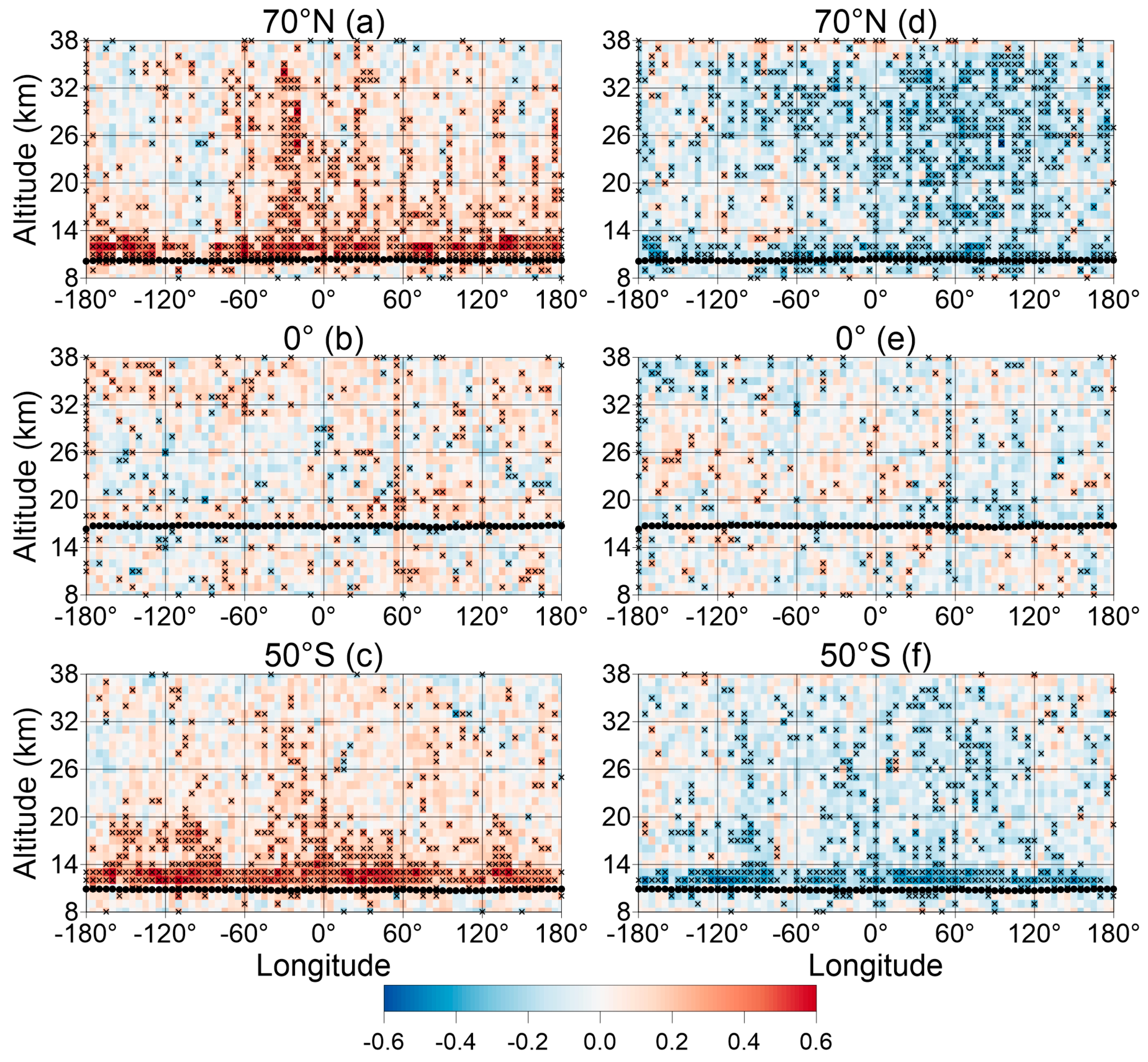
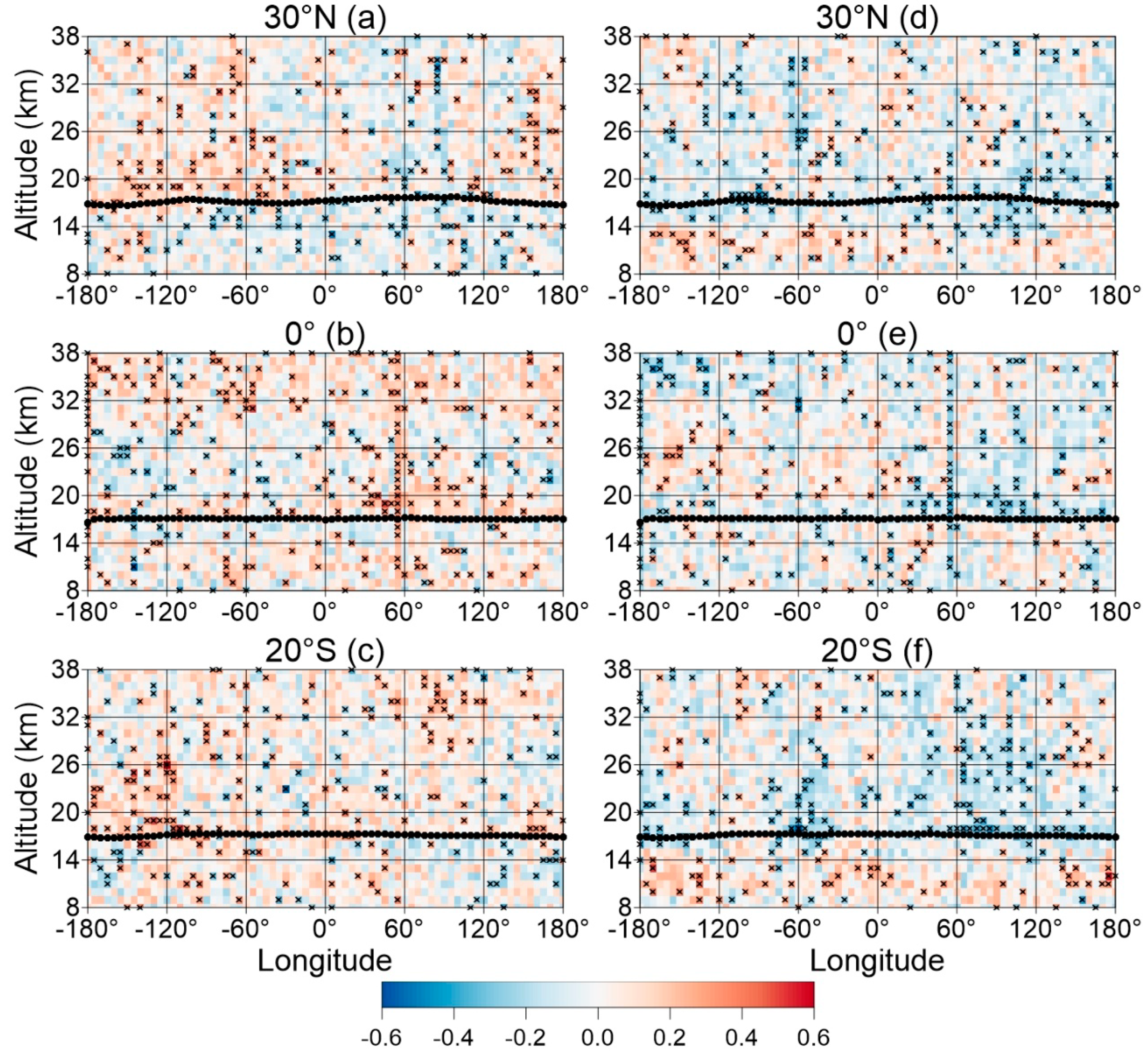
3.3. The Horizontal Structures of the Correlations Between Ep and Tropopause Parameters

The horizontal structures of the correlations between GW Ep values and the tropopause parameters are investigated in this section. Figure 3 reveals that over different latitudes, the correlation coefficients between Ep values and LRT-H/LRT-T that are statistically significant are generally positive/negative. Figure 5 further shows the distributions of the peak positive/negative correlation coefficients between Ep values and LRT-H/LRT-T and the corresponding heights where these peak correlation coefficients were calculated based on the 5° × 5° longitude-latitude grids.
From Figure 5a,b, it can be seen that in the tropics, the peak positive correlation coefficients between GW Ep values and LRT-H are generally smaller than 0.4, which are calculated at the heights between 14 km and 38 km. The distributions of both the peak correlation coefficients and the corresponding heights were dispersed. In the middle and high latitudes, the latitudinal distribution of the peak correlation coefficients between GW Ep values and LRT-H were distinct. Over the latitudes 45° N–75° N, most of the peak correlation coefficients between GW Ep values and LRT-H were between 0.5 and 0.8, and the corresponding heights were mainly located above the LRT at 11 km to 14 km. While over 45° S–75° S latitudes, most of the peak correlation coefficients were around 0.6, and the corresponding height were also mainly located above the LRT. Compared with the same latitudes in the NH, the peak positive correlation coefficients between GW Ep values and LRT-H over the 45° S–75° S latitudes were smaller, and the latitude zone with distinct peak correlation coefficients had a poorer continuity and a narrower width. Figure 5a,b show that the distributions of the peak correlation coefficients between Ep and LRT-H in the NH and SH were not symmetrical, while the distributions of the corresponding heights were basically symmetrical.
Figure 5c,d show the distributions of the peak negative correlation coefficients between Ep and LRT-T and the corresponding heights where these peak coefficients were calculated. The horizontal distributions of the peak negative correlation coefficients between Ep values and LRT-T were similar to those of the peak positive correlation coefficients between Ep values and LRT-H. In the tropics, the peak negative correlation coefficients between Ep values and LRT-T were between −0.2 and −0.4 with the corresponding heights mainly at 14 km to 38 km. Over the 45°–75° latitudes in the NH and SH, zonal regions existed where the peak negative correlation coefficients were between −0.4 and −0.6 and the corresponding heights were over the LRT at 11 km to 14 km.
It can be seen from Figure 5 that at middle and high latitudes, the peak positive/negative correlation coefficients between GW Ep and LRT-H/LRT-T were calculated above the LRT at the altitude range of 11 km to 14 km, while in the tropics, the peak correlation coefficients were distributed dispersively at the altitude range between 14 km and 38 km, which is also shown in Figure 3 and Figure 4.
In the following part of this study, we will focus on the correlations between GW Ep at certain altitude ranges near and above the tropopause and the tropopause parameters over the globe. Considering that the height of LRT decreases gradually from the equator to the poles, this altitude range was chosen as 13 km at middle and high latitudes and 17 km–19 km in the tropics. Figure 6a,b shows the global distributions of the correlation coefficients between Ep values and LRT-H, and those between Ep and LRT-T, respectively. The contour plots of the means of outgoing longwave radiation (OLR) during September 2006–May 2013 are also shown in the tropics in the two subfigures. OLR data is downloaded from the Climate Diagnostics Center Website (at http://www.cdc.noaa.gov). The regions where OLR < 240 W/m2 are where deep convections occurred.
Figure 6 shows that the statistically significant correlation coefficients between Ep and LRT parameters present distinct latitudinal distributions at middle and high latitudes, especially between 45° N–75° N and 45° S–75° S. From Figure 6a, it is evident that GW Ep generally has a positive correlation with LRT-H over the globe. At the latitudes of 45° N–75° N and 45° S–75° S, the magnitudes of the correlation coefficients are between 0.3 to 0.6 over the zonal regions where the correlation coefficients are statistically significant. While in the tropics, the correlation coefficients between GW Ep and LRT-H are smaller, which is 0.2–0.3, and the regions where the correlation coefficients pass through the significance test of the confidence level of 95% are where deep convections occur. In the tropics, convection is a main source of GW [26,34], and Ep has a significant correlation with LRT-H over the regions where deep convections occur, which to some extent indicates that the tropopause structure is affected by the convections [39].
The signs of the correlation coefficients between Ep values and LRT-T shown in Figure 6b were opposite to those between Ep values and LRT-H, as shown in Figure 6a. At middle and high latitudes, the statistically significant negative correlation coefficients between Ep values and LRT-T showed distinct latitudinal distributions, while in the tropics, the statistically significant negative correlation coefficients between Ep values and LRT-T were mainly concentrated in the regions where deep convections occur.
Figure 7 shows the temporal variations of the monthly means and the monthly anomalies of GW Ep at 13 km and the LRT parameters at the latitudes of 50° N and 50° S. From Figure 7a, it can be seen that at 50° N, the monthly means of both GW Ep and LRT-H show the same annual cycle with the maximum/minimum values calculated during boreal summer/winter. Although some studies indicated that GW Ep usually became larger in boreal winter and smaller in boreal summer in lower stratosphere at middle and high latitudes using RO data [26,35,40,41], the seasonal cycle of GW Ep over 20 km were investigated in these studies.
Figure 7a reveals that different from the seasonal variation characteristics of GW Ep over 20 km, the GW Ep near and over the tropopause was larger in boreal summer and smaller in boreal winter, which had a positive correlation with the seasonal variation of LRT-H with a statistically significant correlation coefficient of 0.9. Figure 7b shows that the variation pattern of the monthly anomalies of GW Ep at 13 km was similar to that of the LRT-H with a correlation coefficient of 0.61, which passed through the significance test of the confidence level of 99%.
The temporal variations of the monthly means and the monthly anomalies of Ep and LRT-T at 13 km over the latitude 50° S are shown in Figure 7c,d. The seasonal cycle of GW activity was negatively correlated with that of LRT-T with a correlation coefficient of −0.84. The temporal variations of the monthly anomalies of Ep values were also negatively correlated with those of LRT-T with a correlation coefficient of −0.37, which passed through the significance test of the confidence level of 99%.

3.4. The Relationship between Convection and Tropopause in the Tropics

It has been noticed that the tropical tropopause is not only related to atmospheric waves but also related to deep convections [10,42,43]. Figure 6 reveals that in the tropics, the statistically significant correlation coefficients between Ep and LRT parameters were mainly calculated over in the regions where deep convection occurs. In this section, we will focus on the relationship between convection and LRT in the tropics. Figure 8 shows the global distribution of the averaged seasonal means of LRT-H and OLR during 2006 to 2013. The seasons are categorized here as MAM (March/April/May), JJA (June/July/August), SON (September/October/November), and DJF (December/January/February). It can be seen that the LRT-H was higher in DJF and lower in JJA, which is consistent with the seasonal cycle shown in Figure 1a. In MAM and SON, the deep convections were basically symmetric about the equator, and in these regions, the LRT-H was lower, especially in SON, such as the Indian Ocean and Central America. In JJA and DJF, convections are more active in the summer hemisphere than in the winter hemisphere [42]. Figure 8d shows that in DJF, deep convections are accompanied by the lower LRT, such as in Southeast Asia, South Africa and Central South America. In summary, the LRT-H was lower in deep convections in all the four seasons.
Figure 9 shows the global distribution of the averaged seasonal means of LRT-T and OLR during 2006 to 2013. From Figure 9b, it is evident that in JJA, lower LRT temperature is broadly found in the same regions where deep convections occur, such as in India, Southeast Asia and the Western Pacific. Minima in LRT temperature appears over the Western Pacific and extends northward over the south-Asia monsoon circulation near the deep convections. In Central America, the cold LRT and deep convections extend northward to 25° N. The comparison between Figure 8b and Figure 9b shows that in JJA, the low and cold LRT appears in Central America and the Western Pacific, while the high and cold LRT appears in India. In the other three seasons, as revealed by Figure 9a,c,d, the coincidence between low LRT-T and deep convections is even more distinguished than that between LRT-H and deep convections. In summary, the low and cold LRT appears in deep convection regions.
The distribution of OLR and CPT parameters in the tropics is similar to Figure 8 and Figure 9 (Figureures are not shown here), which means that there is strong correspondence between CPT-T/CPT-H and deep convections.
Reference [42] analyzed the distribution and influence of convection in the tropical tropopause region using cold brightness temperatures from satellites and temperatures from contemporaneous reanalysis. They found that there was a significant correspondence locally between the deepest convection and coldest tropopause temperatures. Reference [10] investigated the structure and variability of temperature in the tropical upper troposphere and lower stratosphere using GPS/MET RO data during April 1995 to February 1997. They found that low tropopause is associated with deep convections. Our results are consistent with both of these studies.
The Pearson correlation coefficients between OLR and tropopause parameters over 5° S–5° N latitudes are shown in Table 1. It can be seen that the weakest correlation between OLR and LRT-H/CPT-H is calculated in MAM with a correlation coefficient of −0.12/0.11, which fails to pass the significance test of the confidence level of 95%. While during the same season, strong correlations exist between OLR and LRT-T/CPT-T, as revealed by the correlation coefficient of 0.63/0.64, which passes through the significance test of the confidence level of 99%. In the other three seasons, the correlation coefficients between OLR and tropopause height and temperature are all positive and pass through the significance test of the confidence level of 95%, indicating that a low and cold tropopause is generally associated with deep convections which is presented by low OLR.

4. Discussion

Section 2.1 pointed out that as GWs can cause the perturbations of temperature, the key to calculate the GW Ep by COSMIC RO temperature profiles is the estimation of temperature perturbations ( T ). In the example presented by Figure 1a of reference [34], it is shown that in the tropopause and throughout the stratosphere, there is a “wavy” variability in the COSMIC temperature profile (blue line), and it also appeared in GPS/MET temperature profiles [10,40,44] and radiosonde observations [29]. The “wavy” variability of temperature profile might be attributed to GWs [10,40,44], which indicates that GWs can influence the tropopause temperature. It has been revealed that GWs play a main role in regulating tropopause parameters [18]. The breaking of GWs in the stratosphere transports energy, momentum, chemical, and atmospheric constituents (i.e. water vapor) across the tropopause to the surroundings [45], which affected the tropopause parameters accordingly [18].
In middle and high latitudes, significant correlations between GW Ep and LRT height and temperature appears about several kilometers above the tropopause, as shown by Figure 3, and GW Ep at 13 km has a positive correlation with LRT-H and a negative correlation with LRT-T, as shown by Figure 6. The seasonal cycles of the monthly means and the monthly anomalies of GW Ep and LRT-H/LRT-T shown in Figure 7 reveals that LRT-H/LRT-T increases/decreases with the increase of Ep values in middle and high latitudes. All these results indicate that close relations exist between GWs and LRT parameters in middle and high latitudes, which might be attributed to that LRT is lifted and becomes cooler when GWs propagate from the troposphere to stratosphere.
It is interesting that our results are opposite to that of reference [18], who investigated the relationship between GWs at 17 km and the temperature and height of CPT in Tibet and concluded that the enhancements of GW Ep lead to the increase of CPT-T. The reasons might be attributed to that GW Ep at different height layers are concerned about by reference [18] and by this work.
In the tropics, strong correlation exists between convections and tropopause parameters, which indicates that low and cold tropopause, appears in deep convection regions, as revealed by Figure 8, Figure 9 and Table 1. The result is consistent with references [7,42]. Although this correlation might be a result of convective cooling of the tropopause, or a tropopause cooled by other means such as radiative cooling, the former factor appears more likely [42]. On the other hand, Figure 6 shows that the correlations between GW Ep and tropopause height and temperature are significant in deep convection regions, which indicates that tropopause parameters variability might also have close relationship with GW activity. Reference [7] indicates that radiative forcing might be important for tropical tropopause on monthly time scales, while the majority of tropopause temperature and height variability appears to be related to wave-like variability. They also found that there were significant correlations between GPS/MET temperature and OLR in the tropics, which quantified the influence of deep convection on temperatures in the tropical tropopause region. In summary, the tropopause parameters in the tropics might be affected by both deep convections [7] and the GWs excited by deep convection.

5. Conclusions

In this study, the relationship between gravity wave (GW) potential energy (Ep) and the tropopause height and temperature over the globe was investigated using COSMIC radio occultation (RO) dry temperature profiles during September 2006 to May 2013.
The longitude-altitude cross sections of the Pearson correlation coefficients between Ep and LRT parameters over the globe and those between Ep and CPT parameters over the latitudes 30° S–30° N showed that at middle and high latitudes, concentrated distributions of statistically significant positive (negative) correlation coefficients between GW Ep and LRT-H (LRT-T) were generally calculated in the height range between the LRT and several kilometers above. In the tropics, the distributions of the correlation coefficients between GW Ep and LRT and CPT parameters that are statistically significant were dispersive.
The global distributions of the peak positive/negative correlation coefficients between GW Ep and LRT-H/LRT-T and their corresponding altitudes showed that at middle and high latitudes, most of the peak positive/negative correlation coefficients between GW Ep and LRT-H/LRT-T were around 0.5~0.8/−0.4~−0.6, which were calculated over the altitudes of 10~14 km with distinct zonal distribution characteristics, while in the tropics, the peak correlation coefficients, which are only 0.2~0.4/−0.2~−0.4, were calculated dispersively over the altitudes of 14~38 km. At middle and high latitudes, the statistically significant positive/negative correlation coefficients between GW Ep over the altitude of 13 km and LRT-H/LRT-T present distinct zonal distribution features, while in the tropical regions, statistically significant positive/negative correlations existed between GW Ep over the altitude of 17~19 km and LRT-H/LRT-T where deep convections occur.
At the latitudes 50° N and 50° S, the temporal variations of the monthly means and the monthly anomalies of the LRT parameters and GW Ep over the altitude of 13 km show that LRT-H/LRT-T increases/decreases with the increase of Ep, which might be attributed to that LRT is lifted and becomes cooler when GWs propagate from the troposphere to the stratosphere. The distribution of 2006–2013 averaged seasonal means of OLR and LRT parameters over the tropics and the correlation coefficients between OLR and LRT parameters over 5°S–5°N show that strong correlations between convections and the tropopause parameters exist in most seasons over the tropics, which indicates that low and cold tropopause appears in deep convection regions. It can be concluded that GW activities affects the variations of the tropopause parameters. At middle and high latitudes, the tropopause was lifted and becomes cooler when GWs propagate from the troposphere to stratosphere, while in the tropics, both deep convections and GWs excited accordingly had impacts on the tropopause structure.

Author Contributions

D.Y., X.X., and J.L. (Jia Luo) conceptualized the initial idea and experiment design; D.Y. analyzed the data; D.Y., X.X. and J.L. (Jia Luo) wrote the main manuscript text; J.L. (Jia Luo) and J.L. (Juan Li) contributed grammar correcting of the text.

Funding

This work was supported by the National Natural Science Foundation of China (Grant No. 41774033 and 41774032) and the National Basic Research Program of China (973 Program) (Grant No. 2013CB733302).

Acknowledgments

The authors would like to thank UCAR for providing COSMIC RO data through CDAAC, and NOAA for providing OLR data through the Climate Diagnostics Center.

Conflicts of Interest

The authors declare no conflict of interests.

References

  1. Son, S.W.; Tandon, N.F.; Polvani, L.M. The fine-scale structure of the global tropopause derived from COSMIC GPS radio occultation measurements. J. Geophys. Res. 2011, 116, D20113. [Google Scholar] [CrossRef]
  2. Holton, J.R.; Haynes, P.H.; McIntyre, M.E.; Douglass, A.R.; Rood, R.B.; Pfister, L. Stratosphere-troposphere exchange. Rev. Geophys. 1995, 33, 403–439. [Google Scholar] [CrossRef]
  3. Sausen, R.; Santer, B.D. Use of changes in tropopause height to detect human influences on climate. Meteorol. Z. 2003, 12, 131–136. [Google Scholar] [CrossRef]
  4. Schmidt, T.; de la Torre, A.; Wickert, J. Global gravity wave activity in the tropopause region from CHAMP radio occultation data. Geophys. Res. Lett. 2008, 35, 428–451. [Google Scholar] [CrossRef]
  5. Schmidt, T.; Beyerle, G.; Heise, S.; Wickert, J.; Rothacher, M. A climatology of multiple tropopauses derived from GPS radio occultations with CHAMP and SAC-C. J. Geophys. Res. Lett. 2006, 33, L04808. [Google Scholar] [CrossRef]
  6. Liu, Y.; Xu, T.; Liu, J. Characteristics of the seasonal variation of the global tropopause revealed by COSMIC/GPS data. Adv. Space Res. 2014, 54, 2274–2285. [Google Scholar] [CrossRef]
  7. Randel, W.J.; Jensen, E.J. Physical processes in the tropical tropopause layer and their roles in a changing climate. Nat. Geosci. 2013, 6, 169–176. [Google Scholar] [CrossRef]
  8. Yulaeva, E.; Holton, J.; Wallace, J. On the cause of the annual cycle in tropical lower-stratospheric temperatures. J. Atmos. Sci. 1994, 51, 169–174. [Google Scholar] [CrossRef]
  9. Zhou, X.; Holton, J.R. Intraseasonal Variations of Tropical Cold-Point Tropopause Temperatures. J. Clim. 2002, 15, 1460–1473. [Google Scholar] [CrossRef]
  10. Randel, W.J.; Wu, F.; Ríos, W.R. Thermal variability of the tropical tropopause region derived from GPS/MET observations. J. Geophys. Res. 2003, 108, 4020. [Google Scholar] [CrossRef]
  11. Seidel, D.J.; Randel, W.J. Variability and trends in the global tropopause estimated from radiosonde data. J. Geophys. Res. 2006, 111, D21101. [Google Scholar] [CrossRef]
  12. Son, S.W.; Lee, S. Intraseasonal Variability of the Zonal-Mean Tropical Tropopause Height. J. Atmos. Sci. 2007, 64, 2695–2706. [Google Scholar] [CrossRef]
  13. Tsuda, T.; Murayama, Y.; Wiryosumarto, H.; Harijono, S.W.B.; Kato, S. Radiosonde observations of equatorial atmosphere dynamics over Indonesia: 2. Characteristics of gravity waves. J. Geophys. Res. 1994, 99, 10507–10516. [Google Scholar] [CrossRef]
  14. Boehm, M.T.; Verlinde, J. Stratospheric influence on upper tropospheric tropical cirrus. Geophys. Res. Lett. 2000, 27, 3209–3212. [Google Scholar] [CrossRef] [Green Version]
  15. Satheesan, K.; Murthy, B.V.K. Modulation of tropical tropopause by wave disturbances. J. Atmos. Sol-Terr. Phys. 2005, 67, 878–883. [Google Scholar] [CrossRef]
  16. Jain, A.R.; Das, S.S.; Mandal, T.K.; Mitra, A.P. Observations of extremely low temperature over the Indian tropical region during monsoon and post monsoon months: Possible implications. J. Geophys. Res. 2006, 111, D07106. [Google Scholar] [CrossRef]
  17. Das, S.S.; Kumar, K.K.; Uma, K.N. MST radar investigation on inertia-gravity waves associated with tropical depression in the upper troposphere and lower stratosphere over Gadanki (13.5 degrees N, 79.2 degrees E). J. Atmos. Sol-Terr. Phys. 2010, 72, 1184–1194. [Google Scholar]
  18. Khan, A.; Jin, S. Effect of Gravity Waves on the Tropopause Temperature, Height and Water Vapor in Tibet from COSMIC GPS Radio Occultation Observations. J. Atmos. Sol-Terr. Phys. 2016, 138, 23–31. [Google Scholar] [CrossRef]
  19. Zhang, Y.; Zhang, S.; Huang, C.; Huang, K.; Gong, Y.; Gan, Q. The interaction between the tropopause inversion layer and the inertial gravity wave activities revealed by radiosonde observations at a midlatitude station. J. Geophys. Res. 2015, 120, 8099–8111. [Google Scholar] [CrossRef] [Green Version]
  20. Moustaoui, M.; Joseph, B.; Teitelbaum, H. Mixing layer formation near the tropopause due to gravity wave-critical level interactions in a cloud-resolving model. J. Atmos. Sci. 2004, 61, 3112–3124. [Google Scholar] [CrossRef]
  21. Wang, L.; Alexander, M.J. Global estimates of gravity wave parameters from GPS radio occultation temperature data. J. Geophys. Res. 2010, 115, D21122. [Google Scholar] [CrossRef]
  22. Seidel, D.J.; Rebecca, J.R.; James, K.A. Climatological characteristics of the tropical tropopause as revealed by radiosondes. J. Geophys. Res. 2001, 106, 7857–7878. [Google Scholar] [CrossRef] [Green Version]
  23. Schmidt, T.; Wickert, J.; Beyerle, G.; Reigber, C. Tropical tropopause parameters derived from GPS radio occultation measurements with CHAMP. J. Geophys. Res. 2004, 109, D13105. [Google Scholar] [CrossRef]
  24. Sivakumar, V.; Bencherif, H.; Bègue, N.; Thompson, A.M. Tropopause characteristics and variability from 11 yr of SHADOZ observations in the southern tropics and subtropics. J. Appl. Meteorol. Climatol. 2011, 50, 1403–1416. [Google Scholar] [CrossRef]
  25. Xu, X.; Gao, P.; Zhang, X. Global multiple tropopause features derived from COSMIC radio occultation data during 2007 to 2012. J. Geophys. Res. 2014, 119, 8515–8534. [Google Scholar] [CrossRef] [Green Version]
  26. Ratnam, M.V.; Tetzlaff, G.; Jacobi, C. Global and seasonal variations of stratospheric gravity wave activity deduced from the CHAMP/GPS satellite. J. Atmos. Sci. 2004, 61, 1610–1620. [Google Scholar] [CrossRef]
  27. Hindley, N.P.; Wright, C.J.; Smith, N.D.; Mitchell, N.J. The southern stratospheric gravity wave hot spot: individual waves and their momentum fluxes measured by COSMIC GPS-RO. Atmos. Chem. Phys. 2015, 15, 7797–7818. [Google Scholar] [CrossRef] [Green Version]
  28. Das, S.S.; Jain, A.R.; Kumar, K.K.; Rao, D.N. Diurnal variability of the tropical Tropopause: Significance of VHF radar measurements. Radio Sci. 2008, 43, RS6003. [Google Scholar] [CrossRef]
  29. Nishida, M.; Shimizu, A.; Tsuda, T.; Rocken, C.; Ware, R.H. Seasonal and longitudinal variations in the tropical tropopause observed with the GPS occultation technique (GPS/MET). J. Meteorol. Soc. Jpn. 2000, 78, 691–700. [Google Scholar] [CrossRef]
  30. Alexander, S.P.; Tsuda, T.; Kawatani, Y. COSMIC GPS observations of Northern Hemisphere winter stratospheric gravity waves and comparisons with an atmospheric general circulation model. Geophys. Res. Lett. 2008, 35, L10808. [Google Scholar] [CrossRef]
  31. Schmidt, T.; Alexander, P.; de la Torre, A. Stratospheric gravity wave momentum flux from radio occultations. J. Geophys. Res. 2016, 121, 4443–4467. [Google Scholar] [CrossRef] [Green Version]
  32. Wang, L.; Alexander, M.J. Gravity wave activity during stratospheric sudden warmings in the 2007–2008 Northern Hemisphere winter. J. Geophys. Res. 2009, 114, D18108. [Google Scholar] [CrossRef]
  33. Stockwell, R.G.; Mansinha, L.; Lowe, R.P. Localisation of the complex spectrum: The S-transform. IEEE Trans. Signal Process. 1996, 44, 998–1001. [Google Scholar] [CrossRef]
  34. Xu, X.; Yu, D.; Luo, J. Seasonal variations of global stratospheric gravity wave activity revealed by COSMIC RO data. In Proceedings of the CPGPS 2017 Forum on Cooperative Positioning and Service, Harbin, China, 19–21 May 2017. [Google Scholar]
  35. Xu, X.; Yu, D.; Luo, J. The spatial and temporal variability of global stratospheric gravity waves and their activity during SSW revealed by COSMIC measurements. Adv. Atmos. Sci. 2018, 35, 1533–1546. [Google Scholar] [CrossRef]
  36. Khandu; Awange, J.L.; Forootan, E. Interannual variability of temperature in the UTLS region over Ganges-Brahmaputra-Meghna river basin based on COSMIC GNSS RO data. Atmos. Meas. Tech. 2016, 9, 1685–1699. [Google Scholar] [CrossRef]
  37. Mohanakumar, K. Stratosphere Troposphere Interactions; Springer: London, UK, 2008. [Google Scholar]
  38. Kim, J.; Son, S.W. Tropical Cold-Point Tropopause: Climatology, Seasonal Cycle and Intraseasonal Variability derived from COSMIC GPS Radio Occultation Measurements. J. Clim. 2012, 25, 5343–5360. [Google Scholar] [CrossRef]
  39. Ratnam, M.V.; Tsuda, T.; Kozu, T.; Mori, S. Long-term behavior of the Kelvin waves revealed by CHAMP/GPS RO measurements and their effects on the tropopause structure. Ann. Geophys. 2006, 24, 1355–1366. [Google Scholar] [CrossRef] [Green Version]
  40. Tsuda, T.; Nishida, M.; Rocken, C.; Ware, R.H. A global morphology of gravity wave activity in the stratosphere revealed by the GPS occultation data (GPS/MET). J. Geophys. Res. 2000, 105, 7257–7273. [Google Scholar] [CrossRef]
  41. Faber, A.; Llamedo, P.; Schmidt, T.; de la Torre, A.; Wickert, J. On the Determination of Gravity Wave Momentum Flux from GPS Radio Occultation Data. Atmos. Meas. Tech. 2013, 6, 3169–3180. [Google Scholar] [CrossRef]
  42. Gettelman, A.; Salby, M.L.; Sassi, F. Distribution and influence of convection in the tropical tropopause region. J.Geophys. Res. 2002, 107, 4080. [Google Scholar] [CrossRef]
  43. Ryu, J.H.; Lee, S.; Son, S.W. Vertically Propagating Kelvin Waves and Tropical Tropopause Variability. J. Atmos. Sci. 2007, 65, 1817–1837. [Google Scholar] [CrossRef]
  44. Alexander, M.J.; Tsuda, T.; Vincent, R.A. Latitudinal variations observed in gravity waves with short vertical wavelengths. J. Atmos. Sci. 2002, 59, 1394–1404. [Google Scholar] [CrossRef]
  45. Wang, P.K. Moisture plumes above thunderstorm anvils and their contributions to cross-tropopause transport of water vapor in midlatitudes. J. Geophys. Res. 2003, 108, 4194. [Google Scholar] [CrossRef]
Figure 1. Time-latitude plots of monthly means of (a) lapse rate tropopause height (LRT-H), (b) lapse rate tropopause temperature (LRT-T), (c) cold point tropopause height (CPT-H), and (d) cold point tropopause temperature (CPT-T).
Atmosphere 10 00075 g001
Figure 2. (a) The monthly means and (b) the monthly anomalies time series of gravity wave potential energy (GW Ep) at 13 km and the LRT-H over the grid (50° N, 25° W).
Atmosphere 10 00075 g002
Figure 3. Longitude-altitude cross sections of Pearson correlation coefficients between Ep and LRT-H (left column), and between Ep and LRT-T (right column) at (a,d) 70° N, (b,e) 0° and (c,f) 50° S. The regions where the correlation coefficients pass through the significance test of the confidence level of 95% are marked with crosses. The LRT height is represented by black dotted lines (af).
Atmosphere 10 00075 g003
Figure 4. Longitude-altitude cross sections of Pearson correlation coefficients between Ep and CPT-H (left column), and between Ep and CPT-T (right column) at (a,d) 30° N, (b,e) 0°, and (c,f) 30° S. The regions where the correlation coefficients pass through the significance test of the confidence level of 95% are marked with crosses. The CPT height is represented by black dotted lines (af).
Atmosphere 10 00075 g004
Figure 5. The peak positive/negative correlation coefficients between Ep and (a) LRT-H, (c) LRT-T. The height at which these peak correlation coefficients between Ep and (b) LRT-H, (d) LRT-T are calculated.
Atmosphere 10 00075 g005
Figure 6. The global distribution of the correlation coefficients between Ep and (a) LRT-H, and (b) LRT-T. The height layer between 30° S–30° N is 17–19 km, and in middle and high latitudes is 13 km. The red solid line and the red dashed line represents OLR = 240 W/m2 and OLR = 220 W/m2, respectively. The regions where the correlation coefficients pass through the significance test of the confidence level of 95% are marked with crosses.
Atmosphere 10 00075 g006
Figure 7. (a) The monthly means and (b) the monthly anomalies time series of GW Ep at 13 km and the LRT-H at 50° N. (c) The monthly means and (d) the monthly anomalies time series of GW Ep at 13 km and the LRT-T at 50° S.
Atmosphere 10 00075 g007
Figure 8. Global distribution of 2006–2013 averaged seasonal means ((a) MAM, (b) JJA, (c) SON, and (d) DJF) of LRT-H and OLR. The red solid line and the red dashed line represents OLR = 240 W/m2 and OLR = 220 W/m2, respectively.
Atmosphere 10 00075 g008
Figure 9. Global distribution of 2006–2013 averaged seasonal means ((a) MAM, (b) JJA, (c) SON, and (d) DJF) of LRT-T and OLR. The red solid line represents OLR = 240 W/ m2, and the red dashed line represents OLR = 220 W/m2.
Atmosphere 10 00075 g009
Table 1. The Pearson correlation coefficient (CC) and the corresponding confidence level (CL) between OLR and the tropopause parameters over 5° S–5° N in each season during 2006–2013.
SeasonOLR and LRT-HOLR and LRT-TOLR and CPT-HOLR and CPT-T
CCCLCCCLCCCLCCCL
MAM−0.1267.8%0.6399.9%0.1160.7%0.6499.9%
JJA0.6299.9%0.3499.6%0.5799.9%0.3799.9%
SON0.4099.9%0.5299.9%0.4699.9%0.5499.9%
DJF0.2697.4%0.5499.9%0.4499.9%0.5699.9%

