Forecasting of Surface Ozone Concentration by Using Artificial Neural Networks in Rural and Urban Areas in Central Poland

Abstract
1. Introduction
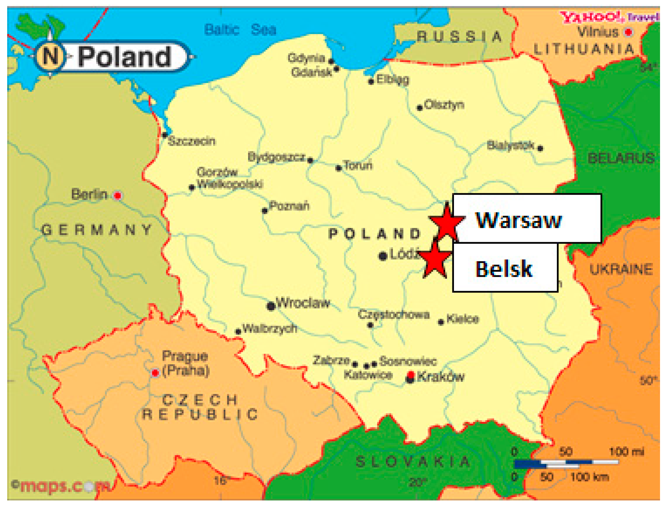
2. Data
3. Methods
- (1)
- Determination of the forecast value of basic meteorological parameters for the period April–September 2014 and April–September 2015 by using the global numerical weather forecast model WRF-ARW. The predicted values (for the next day) included the following parameters: temperature of the air (°C; T), solar radiation (W/m2; SR), wind speed (m/s; WS), and relative humidity (%; RH). These meteorological parameters were predicted with a frequency of 3 h (for 2014) and with a frequency of 1 h (for 2015).
- (2)
- Creation of a data set containing the daily maximum 1-h value of meteorological parameters during the day.
- (3)
- Adding 2 additional variables to the existing data set:
- the number of the month for which surface ozone prediction was carried out (April, 4; May, 5; etc.)
- the maximum hourly mean value of surface ozone concentration within 24 h on the day preceding the forecast
- (4)
- Implementing a complete data set in the Neural Networks package of the Statistica 10 Program. The input variables of the model were the six selected parameters, while the values of these variables for each day of the analyzed period were the cases of the model.
- (5)
- Division of the entire data set into training (70% of cases), test (15%), and validation (15%) subsets.
- (1)
- Prediction error values for each subset. Most attention was paid to errors in the validation and testing subsets as they were independent and not participating in the learning process.
- (2)
- Correlation coefficient values for measured values of surface ozone concentration from the neural network and reality.
4. Results
4.1. Global Sensitivity Analysis
4.2. Quality Assessment of Generated Neural Prognostic Models
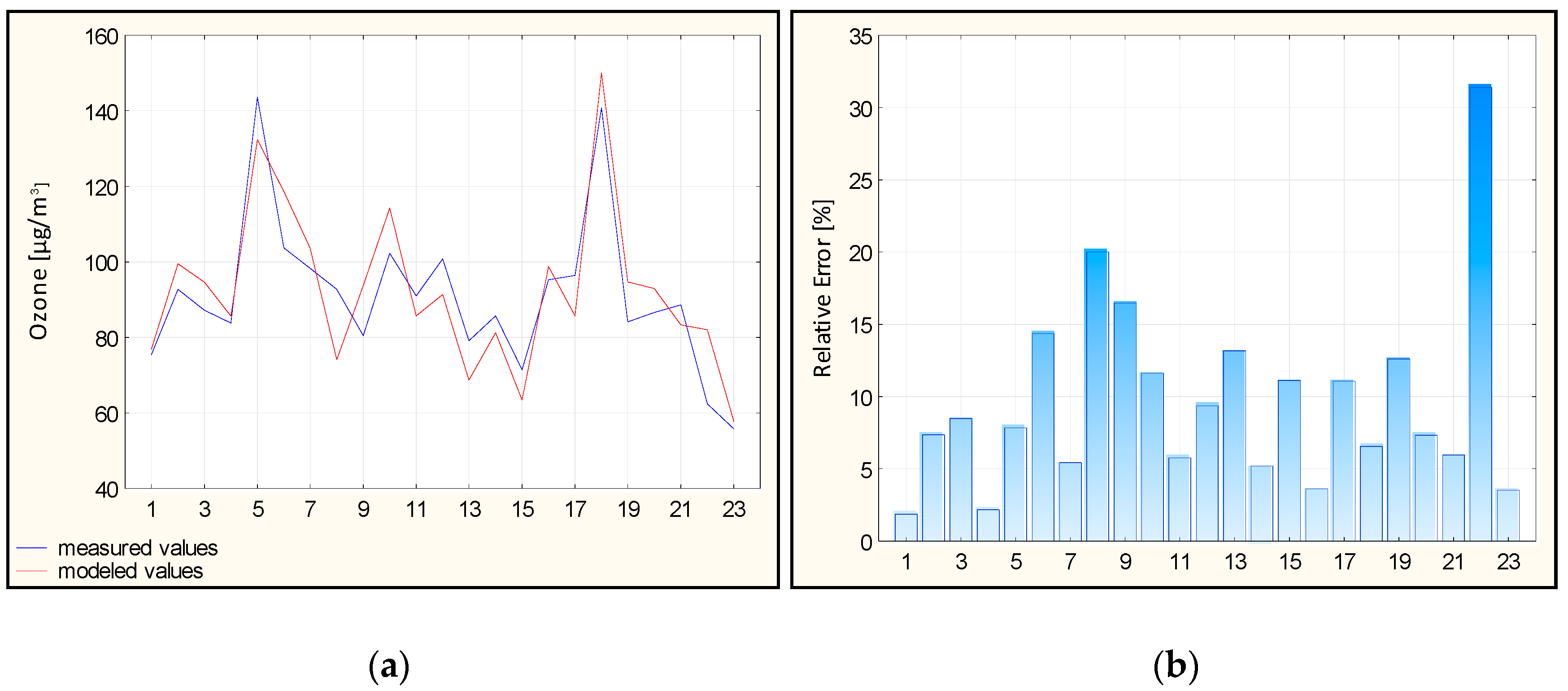
4.3. Results of Ozone Concentration Prediction for Belsk and Warsaw Stations
- performing the test of normality of the data sets to determine whether the data are well characterized by a normal distribution (Shapiro–Wilk test, available in STATISTICA)
- performing the test of statistical significance (parametric or non-parametric) to determine whether the differences in the two analyzed groups are statistically significant. If the conditions for the existence of a normal distribution and homogeneity of the variances in the analyzed data sets are met, we can use parametric tests (t-test). In the case when the assumptions regarding the applicability of the parametric test are not met, we can perform nonparametric tests that do not depend on the shape of distribution.
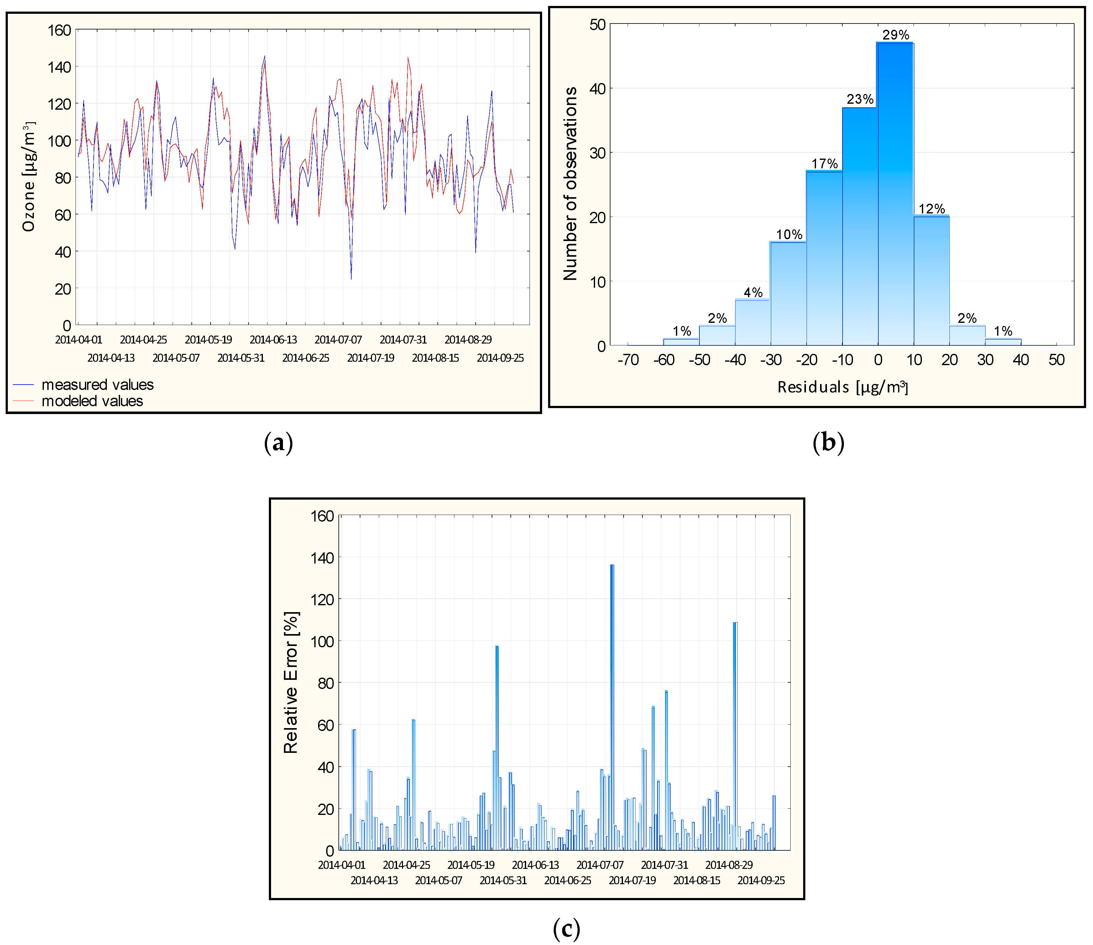
4.4. Prediction of the Maximum 1-h Surface Ozone Concentration Value for 2014
4.5. Analysis of Days with Extremely Bad Forecasts
- for Belsk: for all six cases, the relative error value decreased, wherein for two cases, the predicted values were characterized by relative error values below 50%.
- for Warsaw: for all six cases, the relative error value decreased, wherein for three cases, the value decreased below 50%.
5. Conclusions
- The artificial neural network models developed for forecasting of surface ozone concentration present good statistical compatibility with the measured data in both rural and urban conditions.
- In accordance with the global sensitivity analysis, the most important input variable is the air temperature followed by the number of the month, solar radiation, and the maximum ozone concentration value on the previous day.
- The majority of the highest deviations (with relative error value >50%) from the measured ozone concentration values noted at both Belsk and Warsaw stations (6 and 6 days, respectively) resulted from overestimation of relatively low surface ozone concentrations. Usually, they were associated with a sudden, significant drop of surface ozone concentration values from day to day. In most cases, the direction of the prediction was correct, but the network did not manage the forecast of such low values.
- The forecasts of the high values of surface ozone concentration (approximately 150 µg/m3) present very good statistical compliance with the measured data.
- Possible reasons of overestimation of the lowest surface ozone concentration values could be associated with the quality of forecasts of the input variables, or a training subset that is too small to present all possible variations.
Author Contributions
Funding
Acknowledgments
Conflicts of Interest
References
- Crutzen, P. A discussion of the chemistry of some minor constituents in the stratosphere and troposphere. Pure Appl. Geophys. 1973, 106, 1385–1399. [Google Scholar] [CrossRef]
- Levy, H., II. Normal atmosphere: Large radical and formaldehyde concentrations predicted. Science 1971, 173, 141–143. [Google Scholar] [CrossRef] [PubMed]
- Danielsen, E. Stratospheric-tropospheric exchange based on radioactivity, ozone and potential vorticity. J. Atmos. Sci. 1968, 25, 502–518. [Google Scholar] [CrossRef]
- Moore, G.W.K.; Semple, J.L. High concentration of surface ozone observed along the Khumbu Valley Nepal, April 2007. Geophys. Res. Lett. 2009, 36, L14809. [Google Scholar] [CrossRef]
- Logan, J.A. Tropospheric Ozone: Seasonal Behavior, Trends, and Antropogenic Influence. J. Geophys. Res. 1985, 90, 10463–10482. [Google Scholar] [CrossRef]
- Stohl, A.; Bonasoni, P.; Cristofanelli, P.; Collins, W.; Feichter, J.; Frank, A.; Forster, C.; Gerasopoulos, E.; Gäggeler, H.; James, P.; et al. Stratosphere-troposphere exchange: A review, and what we have learned from STACCATO. J. Geophys. Res. 2003, 108, 8516. [Google Scholar] [CrossRef]
- Stevenson, D.S.; Dentener, F.J.; Schultz, M.G.; Ellingsen, K.; van Noije, T.P.C.; Wild, O.; Zeng, G.; Amann, M.; Atherton, C.S.; Bell, N.; et al. Multimodel ensemble simulations of present-day and near-future tropospheric ozone. J. Geophys. Res. 2006, 111, 1–23. [Google Scholar] [CrossRef]
- Dueñas, C.; Fernández, M.C.; Cañete, S.; Carretero, J.; Liger, E. Analyses of ozone in urban and rural sites in Malaga (Spain). Chemosphere 2004, 56, 631–639. [Google Scholar] [CrossRef] [PubMed]
- Pawlak, I.; Jarosławski, J. The influence of selected meteorological parameters on the concentration of surface ozone in the central region of Poland. Atmos.-Ocean 2015, 53, 126–139. [Google Scholar] [CrossRef]
- The Royal Society. Ground-level Ozone in the 21st Century: Future Trends, Impacts and Policy Implications. Royal Society Policy Document 15/08, RS1276. 2008. Available online: https://royalsociety.org/~/media/Royal_Society_Content/policy/publications/2008/7925.pdf (accessed on 1 January 2018).
- Selin, N.E.; Wu, S.; Nam, K.M.; Reilly, J.M.; Paltsev, S.; Prinn, R.G.; Webster, M.D. Global health and economic impacts of future ozone pollution. Environ. Res. Lett. 2009, 4, 1–9. [Google Scholar] [CrossRef]
- Avnery, S.; Mauzerall, D.L.; Liu, J.; Horowitz, L.W. Global crop yield reductions due to surface ozone exposure: 2. Year 2030 potential crop production losses and economic damage under two scenarios of O3 pollution. Atmos. Environ. 2011, 45, 2297–2309. [Google Scholar] [CrossRef]
- Cataldo, F.; Rosati, A.; Lilla, E.; Ursini, O. On the action of ozone at high concentration on various grades of polyethylene and certain straight chain paraffins. Polym. Degrad. Stab. 2011, 96, 955–964. [Google Scholar] [CrossRef]
- Myhre, G.; Shindell, D.; Bréon, F.M.; Collins, W.; Fuglestvedt, J.; Huang, J.; Koch, D.; Lamarque, J.F.; Lee, D.; Mendoza, B.; et al. Anthropogenic and Natural Radiative Forcing. In Climate Change 2013: The Physical Science Basis. Contribution of Working Group I to the Fifth Assessment. Report of the Intergovernmental Panel on Climate Change; Stocker, T.F., Qin, D., Plattner, G.-K., Tignor, M., Allen, S.K., Boschung, J., Nauels, A., Xia, Y., Bex, V., Midgley, P.M., Eds.; Cambridge University Press: Cambridge, UK; New York, NY, USA, 2013; pp. 659–740. [Google Scholar]
- Staehelin, J.; Harris, N.R.P.; Appenzeller, C.; Eberhard, J. Ozone Trends: A Review. Peviews Geophys. 2001, 39, 231–290. [Google Scholar] [CrossRef]
- Kandil, M.; Gadallach, A.; Tawfik, F.; Kandil, N. Prediction of maximum Ground Ozone Levels using Neural Network. Int. J. Comput. Digit. Sysyt. 2014, 3, 133–140. [Google Scholar] [CrossRef]
- Vautard, R.; Beekmann, M.; Roux, J.; Gombert, D. Validation of a Hybrid Forecasting System for the Ozone Concentrations over the Paris Area. Atmos. Environ. 2001, 35, 2449–2461. [Google Scholar] [CrossRef]
- Hubbard, M.C.; Cobourn, W.G. Development of a Regression Model to Forecast Ground-level Ozone Concentration in Louisville, KY. J. Atmos. Environ. 1998, 32, 2637–2647. [Google Scholar] [CrossRef]
- Barrero, M.A.; Grimalt, J.O.; Cantón, L. Prediction of daily ozone concentration maxima in the urban atmosphere. Chemom. Intell. Lab. Syst. 2006, 80, 67–76. [Google Scholar] [CrossRef]
- Ghazali, N.A.; Ramli, N.A.; Yahaya, A.S.; Yusof, N.F.; Sansuddin, N.; Madhoun, W.A. Transformation of nitrogen dioxide into ozone and prediction of ozone concentrations using multiple linear regression techniques. Environ. Monitor. Assess. 2010, 165, 475–489. [Google Scholar] [CrossRef]
- Gardner, M.W.; Dorling, S.R. Statistical surface ozone models: An improved methodology to account for non-linear behaviour. Atmos. Environ. 2000, 34, 21–34. [Google Scholar] [CrossRef]
- Ryan, W.F. Forecasting Severe Ozone Episodes in the Baltimore Metropolitan Area. Atmos. Environ. 1995, 29, 2387–2398. [Google Scholar] [CrossRef]
- McCulloch, W.S.; Pitts, W.H. A logical calculus of the ideas immanent in nervous activity. Bull. Math. Biophys. 1943, 5, 115–133. [Google Scholar] [CrossRef]
- Guardani, R.; Nascimento, C.A.O.; Gurdani, M.L.G.; Martins, M.H.R.B.; Romano, J. Study of atmospheric ozone formation by means of a neural network-based model. J. Air Waste Manag. Assoc. 1999, 49, 316–323. [Google Scholar] [CrossRef] [PubMed]
- Elkamel, A.; Abdul-Wahab, S.; Bouhamra, W.; Alper, E. Measurement and prediction of ozone levels around a heavily industrialized area: A neural network approach. Adv. Environ. Res. 2001, 5, 47–59. [Google Scholar] [CrossRef]
- Spellman, G. An application of artificial neural networks to the prediction of surface ozone concentrations in the United Kingdom. Appl. Geogr. 1999, 19, 123–136. [Google Scholar] [CrossRef]
- Sousa, S.I.V.; Martins, F.G.; Alvim-Ferraz, M.C.M.; Pereira, M.C. Multiple linear regression and artificial neural networks based on principal components to predict ozone concentrations. Environ. Model. Softw. 2007, 22, 97–103. [Google Scholar] [CrossRef]
- Prybutok, V.R.; Yi, J.; Mitchell, D. Comparison of neural network models with ARIMA and regression models for prediction of Houston’s daily maximum ozone concentrations. Eur. J. Oper. Res. 2000, 122, 31–40. [Google Scholar] [CrossRef]
- Yi, J.; Prybutok, V.R. A neural network forecasting for prediction of daily maximum ozone concentration in an industrialized urban area. Environ. Pollut. 1996, 92, 349–357. [Google Scholar] [CrossRef]
- Chaloulakou, A.; Saisana, M.; Spyrellis, N. Comparative assessment of neural networks and regression models for forecasting summertime ozone in Athens. Sci. Total Environ. 2003, 313, 1–13. [Google Scholar] [CrossRef]
- Inal, F. Artificial Neural Network Prediction of Tropospheric Ozone Concentrations in Instambul, Turkey. Clean-Soil Air Water 2010, 38, 897–908. [Google Scholar] [CrossRef]
- Hadjilski, L.; Hopke, P. Application of artificial neural networks to modeling and prediction of ambient ozone concentrations. J. Air Waste Manag. Assoc. 2000, 50, 894–901. [Google Scholar] [CrossRef]
- Faris, H.; Alkasassbeh, M.; Rodan, A. Artificial Neural Networks for Surface Ozone Prediction: Models and Analysis. Pol. J. Environ. Stud. 2014, 23, 341–348. [Google Scholar]
- Comrie, A.C. Comparing Neural Networks and Regression Models for Ozone Forecasting. J. Air Waste Manag. Assoc. 1997, 47, 653–663. [Google Scholar] [CrossRef]
- Skamarock, W.C.; Klemp, J.B.; Dudhia, J.; Gill, D.O.; Barker, D.M.; Duda, M.G.; Huang, X.Y.; Wang, W.; Powers, J.G. A Description of the Advanced Research WRF Version 3. NCAR/TN–475+STR NCAR TECHNICAL NOTE. 2008. Available online: File:///C:/Users/user/Downloads/A_Description_of_the_Advanced_Research_WRF_Version.pdf (accessed on 1 November 2017).
- Goethals, P.L.M.; Dedecker, A.P.; Gabriels, W.; Lek, S.; De Pauw, N. Applications of artificial neural networks predicting macroinvertebrates in freshwaters. Aquat. Ecol. 2007, 41, 491–508. [Google Scholar] [CrossRef]
- Legates, D.R.; McCabe, G.J., Jr. Evaluating the use of “goodness-of-fit” measures in hydrologic and hydroclimatic model validation. Water Resourc. Res. 1999, 35, 233–241. [Google Scholar] [CrossRef]
- Fox, D.G. Judging Air Quality Model Performance: A Summary of the AMS Workshop on Dispersion Model Performance. Bull. Am. Meteorol. Soc. 1981, 62, 599–609. [Google Scholar] [CrossRef]
- Willmott, C.J. Some Comments on the Evaluation of Model Performance. Bull. Am. Meteorol. Soc. 1982, 63, 1309–1313. [Google Scholar] [CrossRef]
- Directive 2008/50/EC of the European Parliament and of the Council of 21 May 2008 on Ambient air Quality and Cleaner air for Europe. OJL 152, 11.6.2008. pp. 1–44. Available online: https://eur-lex.europa.eu/eli/dir/2008/50/oj (accessed on 1 June 2017).


| 1-h Max | Kind of Network | Architecture of the Network | Correlation Coefficient | Prediction Error | Activation Function | |||||
|---|---|---|---|---|---|---|---|---|---|---|
| Training | Test | Validation | Training | Test | Validation | Hidden Layer | Output Layer | |||
| Belsk | MLP | 6-6-1 | 0.92 | 0.87 | 0.88 | 57.9 | 55.9 | 48.6 | Tanh | Linear |
| Warsaw | MLP | 6-4-1 | 0.93 | 0.93 | 0.85 | 48.3 | 66.0 | 66.5 | Tanh | Logistic |
| 1-h Max | Temperature | Solar Radiation | Month | Ozone 1 Day before | Relative Humidity | Wind Speed | ||||||
|---|---|---|---|---|---|---|---|---|---|---|---|---|
| Quotient | Rank | Quotient | Rank | Quotient | Rank | Quotient | Rank | Quotient | Rank | Quotient | Rank | |
| Belsk | 5.32 | 1 | 1.53 | 3 | 2.67 | 2 | 1.25 | 4 | 1.13 | 5 | 1.04 | 6 |
| Warsaw | 5.84 | 1 | 1.68 | 2 | 1.47 | 3 | 1.35 | 4 | 1.14 | 6 | 1.16 | 5 |
| Station/Measure. | [µg/m3] | [µg/m3] | So [µg/m3] | Sa [µg/m3] | R2 | MBE [µg/m3] | MAE [µg/m3] | RMSE [µg/m3] | d2 |
|---|---|---|---|---|---|---|---|---|---|
| Belsk | 91.2 | 92.6 | 19.6 | 20.8 | 0.78 | −1.3 | 8.6 | 9.9 | 0.94 |
| Warsaw | 97.2 | 95.7 | 20.9 | 20.7 | 0.72 | 1.4 | 8.9 | 11.5 | 0.92 |
| Station/Measure | Observation | Model | ||
|---|---|---|---|---|
| Shapiro–Wilk Test | p | Shapiro–Wilk Test | p | |
| Belsk | 0.8845 | 0.012 | 0.9387 | 0.168 |
| Warsaw | 0.9225 | 0.075 | 0.9106 | 0.042 |
| Station/Measure | Mann–Whitney Test | p |
|---|---|---|
| Belsk | −0.1318 | 0.895 |
| Warsaw | 0.2855 | 0.775 |
| Station/Measure | So | Sa | R2 | MBE | MAE | RMSE | d2 | ||
|---|---|---|---|---|---|---|---|---|---|
| Belsk | 91.3 | 96.0 | 20.4 | 20.6 | 0.53 | −4.8 | 12.1 | 15.9 | 0.83 |
| Warsaw | 93.0 | 92.1 | 22.9 | 22.0 | 0.55 | 0.9 | 13.0 | 16.3 | 0.86 |
| Station/Measure | Observation | Model | ||
|---|---|---|---|---|
| Shapiro–Wilk Test | p | Shapiro–Wilk Test | p | |
| Belsk | 0.9955 | 0.912 | 0.9836 | 0.052 |
| Warsaw | 0.9946 | 0.825 | 0.9442 | 0.000 |
| Station/Measure | Levene’s Test | p | t-Test | p |
|---|---|---|---|---|
| Belsk | 0.2903 | 0.590 | −2.0855 | 0.037 |
| Station/Measure | Mann–Whitney Test | p |
|---|---|---|
| Warsaw | 0.92782 | 0.35350 |
| Date | Measured Values [µg/m3] | Forecast 1 | Forecast 2 | ||
|---|---|---|---|---|---|
| Forecast [µg/m3] | Relative Error [%] | Forecast [µg/m3] | Relative Error [%] | ||
| Belsk | |||||
| 2014-04-06 | 61.8 | 97.4 | 57.6 | 96.1 | 55.4 |
| 2014-04-28 | 69.8 | 113.2 | 62.1 | 86.9 | 24.4 |
| 2014-05-29 | 41.1 | 81.0 | 97.1 | 67.6 | 64.4 |
| 2014-07-12 | 24.6 | 58.2 | 136.4 | 54.5 | 121.6 |
| 2014-08-01 | 59.4 | 104.2 | 75.4 | 81.0 | 36.4 |
| 2014-09-01 | 39.0 | 81.4 | 108.8 | 73.2 | 87.7 |
| Warsaw | |||||
| 2014-05-28 | 63.1 | 103.4 | 63.8 | 69.9 | 10.9 |
| 2014-05-29 | 37.8 | 83.1 | 119.9 | 57.1 | 51.0 |
| 2014-06-03 | 34.0 | 60.3 | 77.2 | 54.0 | 58.8 |
| 2014-07-11 | 55.2 | 87.4 | 58.4 | 76.4 | 38.5 |
| 2014-07-12 | 25.7 | 68.4 | 166.0 | 52.3 | 103.3 |
| 2014-09-01 | 53.2 | 85.2 | 60.1 | 58.2 | 9.4 |
© 2019 by the authors. Licensee MDPI, Basel, Switzerland. This article is an open access article distributed under the terms and conditions of the Creative Commons Attribution (CC BY) license (http://creativecommons.org/licenses/by/4.0/).
Share and Cite
Pawlak, I.; Jarosławski, J. Forecasting of Surface Ozone Concentration by Using Artificial Neural Networks in Rural and Urban Areas in Central Poland. Atmosphere 2019, 10, 52. https://doi.org/10.3390/atmos10020052
Pawlak I, Jarosławski J. Forecasting of Surface Ozone Concentration by Using Artificial Neural Networks in Rural and Urban Areas in Central Poland. Atmosphere. 2019; 10(2):52. https://doi.org/10.3390/atmos10020052
Chicago/Turabian StylePawlak, Izabela, and Janusz Jarosławski. 2019. "Forecasting of Surface Ozone Concentration by Using Artificial Neural Networks in Rural and Urban Areas in Central Poland" Atmosphere 10, no. 2: 52. https://doi.org/10.3390/atmos10020052
APA StylePawlak, I., & Jarosławski, J. (2019). Forecasting of Surface Ozone Concentration by Using Artificial Neural Networks in Rural and Urban Areas in Central Poland. Atmosphere, 10(2), 52. https://doi.org/10.3390/atmos10020052