Article

Discontinuities in the Ozone Concentration Time Series from MERRA 2 Reanalysis

Institute of Atmospheric Physics, Czech Academy of Sciences, 14100 Prague, Czech Republic
*
Author to whom correspondence should be addressed.
Atmosphere 2019, 10(12), 812; https://doi.org/10.3390/atmos10120812
Submission received: 17 October 2019 / Revised: 11 December 2019 / Accepted: 12 December 2019 / Published: 14 December 2019
(This article belongs to the Special Issue Ozone Evolution in the Past and Future)

Abstract

:
Artificial discontinuities in time series are a great problem for trend analysis because they influence the values of the trend and its significance. The aim of this paper is to investigate their occurrence in the Modern-Era Retrospective analysis for Research and Applications, version 2 (MERRA 2) ozone concentration data. It is the first step toward the utilization of the MERRA 2 ozone data for trend analysis. We use the Pettitt homogeneity test to search for discontinuities in the ozone time series. We showed the data above 4 hPa are not suitable for trend analyses due to the unrealistic patterns in an average ozone concentration and due to the frequent occurrence of significant discontinuities. Below this layer in the stratosphere, their number is much smaller, and mostly, they are insignificant, and the patterns of the average ozone concentration are explainable. In the troposphere, the number of discontinuities increases, but they are insignificant. The transition from Solar Backscatter Ultraviolet Radiometer (SBUV) to Earth Observing System (EOS) Aura data in 2004 is visible only above 1 hPa, where the data are not suitable for trend analyses due to other reasons. We can conclude the MERRA 2 ozone concentration data can be used in trend analysis with caution only below 4 hPa.

1. Introduction

Ozone is a very important trace gas in the atmosphere because it protects the earth’s biota from harmful ultraviolet radiation. The high scientific interest in atmospheric ozone arose near the beginning of the 1970s in connection with the problem of the possible supersonic transport impact on the ozone layer. After discovering the Antarctic ozone hole [1], the ozone became an important topic of atmospheric research. The origin of the ozone hole is in the chemical reactions of anthropogenic halogen radicals, which destroy ozone [2]. These results led to signing the Montreal Protocol and its amendments, which stopped the production of the ozone-depleting substances (ODS). This protocol has a positive influence on the ozone layer due to the decrease in ODS [3]. There are some signs of the ozone recovery, especially in the upper stratosphere [4]. In addition, all model studies predict future recovery of the ozone layer [5]. The concentration of ODS is not the only factor that influences the ozone layer. In addition, the greenhouse cooling of the stratosphere [6] and changes in the Brewer–Dobson circulation [7] have an impact on the ozone concentration. In such situations, proper trend analysis is necessary for the understanding of the ozone layer behaviour. Trend analysis was done from ground-based data [8,9]. These data are measured at one point, and the number of ground-based measurements of ozone is insufficient, especially in the Southern Hemisphere. Satellite ozone data have broader coverage, and these data are widely used in trend analysis in ozone research [10]. But in some areas, it is impossible to measure ozone (polar night, below dense clouds) by satellite.
On the other hand, the ozone data from reanalysis are temporally and spatially homogeneous, but there is a big question of the suitability of these data for trend analysis due to the occurrence of discontinuities in them [11]. They can be caused by satellite or instrument replacement or by assimilation of not homogenous basic parameters. [12] considered the evaluation of trends from reanalysis to be a challenge. The aim of this paper is to detect grid points in which discontinuities occur with the help of the Pettitt homogeneity test in the MERRA 2 ozone data in the period 1980–2017. Our study can help us to identify where it is possible to use the MERRA 2 reanalysis for trend study. This paper is divided into the following sections: Section 2 describes the data and method, Section 3 provides results, Section 4 discusses the results, and Section 5 concludes our results.

2. Data and Method

In this paper, we used MERRA 2 ozone monthly mean data from 500 hPa up to the top of the model (0.01 hPa) in the period 1980–2017. MERRA 2 reanalysis covers the whole satellite era. It includes substantial upgrades and changes to the data assimilation system and input data in comparison to previous MERRA reanalysis. New constraints are applied to ensure the conservation of global dry-air mass and to close the balance between surface water fluxes (precipitation minus evaporation) and changes in total atmospheric water [13]. The modified gravity wave scheme substantially improves the model representation of the quasi biennial oscillation (QBO) [14,15]. The assimilation of Microwave Limb Sounder (MLS) temperature retrievals at high-pressure levels (higher than 5 hPa) should improve the reanalysis at upper levels. The assimilation of MLS stratospheric ozone profiles and Ozone Monitoring Instrument (OMI) column ozone since the beginning of the Aura mission in late 2004 also improve the representation of fine-scale ozone features, especially in the region around the tropopause [16]. MERRA and MERRA 2 use the Three Dimensional Variational (3D VAR) assimilation process. MERRA 2 uses regular latitude–longitude grids from 1000 to 0.01 hPa (1/2° latitude × 5/8° longitude). Detail description of all reanalyses (included MERRA 2) can be found in ref [17,18].
We did our analysis for each grid point, we did not use any spatial (longitudinal and latitudinal) averages, because, during every averaging, some information is lost. In each grid and each layer, we used the time series of the ozone concentration and applied the Pettitt homogeneity test [19] to look for discontinuity in it. In each grid, the Pettitt test estimates only one main discontinuity, so this procedure is not able to detect multiple discontinuities. The Pettitt test is a nonparametric test. It has been developed to test homogeneity against the shift in a time series. In this approach, a shift point is at T; indicates that the time series can be divided into two subsequences xt (t = 1..T) and xt (t = T + 1,.. N). Thus, probability distribution functions F1(X) and F2(X) can be associated with the two subsequences. In practice, the null hypothesis H0 is F1(X) is equal to F2(X), and the alternative hypothesis H1 is F1(X) is not equal to F2(X). This method also involves a comparison of the observations so that:
Di,j = sgn(xi − xj),
Di, j = 1 if xi > xj,
Di, j = 0 if xi = xj,
Di, j = −1 if xi < xj.
We must compute the statistic:
UT, N = ∑t = 1..Tt = T, N Di,j, t = 1..N
Using the theory on statistic ranks, another KN variable is derived from UT, N This new variable is defined:
KN max abs(UT,N) T = 1..N − 1.
For the test, a probability of exceeding is fixed for a threshold value k given by the formula:
P (KN>K) ≅ 6exp(−6k2)/(N3 + N2).
The null hypothesis, H0 is rejected if the probability of exceedance given in P is less than the significance level α for a one-sided statistic test.
This test is widely used in the climatological research especially for precipitation and temperature analysis [20,21,22]. We searched for temporal occurrence of discontinuities, so in each grid with a discontinuity, we looked for the year of its occurrence, and we were able to detect the discontinuity occurrence in a certain year. We are interested in the spatial distribution of discontinuities as well. So in each layer and month, we constructed the map of their occurrence.
The Pettitt test tells us the year in which the discontinuity in time series occurs. But it does not say how big the discontinuity is or how it can affect trends. Small discontinuities have little impact on the trend analyses. On the other hand, the large one can have a strong trend impact, so we must divide the discontinuities according to their size. We tried to identify which ones were significant (in our case big enough to impact the trend) or insignificant according to this rule: Suppose we have a time series with the length L, and in year x, we observe the discontinuity. We compute the difference between the average before the year x and after this year. If this difference is larger than the variance of time series, we can say that the discontinuity is significant and will have some impact on trends, and we should be careful using this grid point in a trend analysis. This rule should be used mainly in areas with big variance because if the variance is very small, even the small discontinuities can be identified as significant. Another possibility for assessing the size of the discontinuities is the use of the Mann–Whitney test [23] for detecting significant ones. It would be very interesting to compare the results of both methods, and this topic could be solved in the future paper.

3. Results

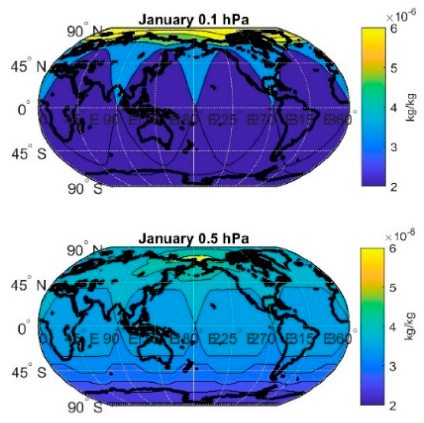
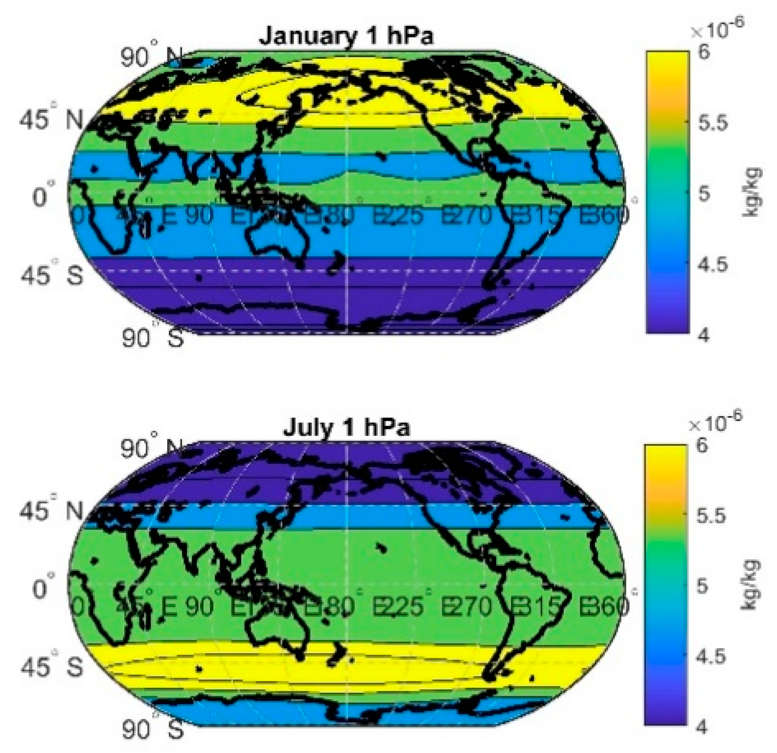
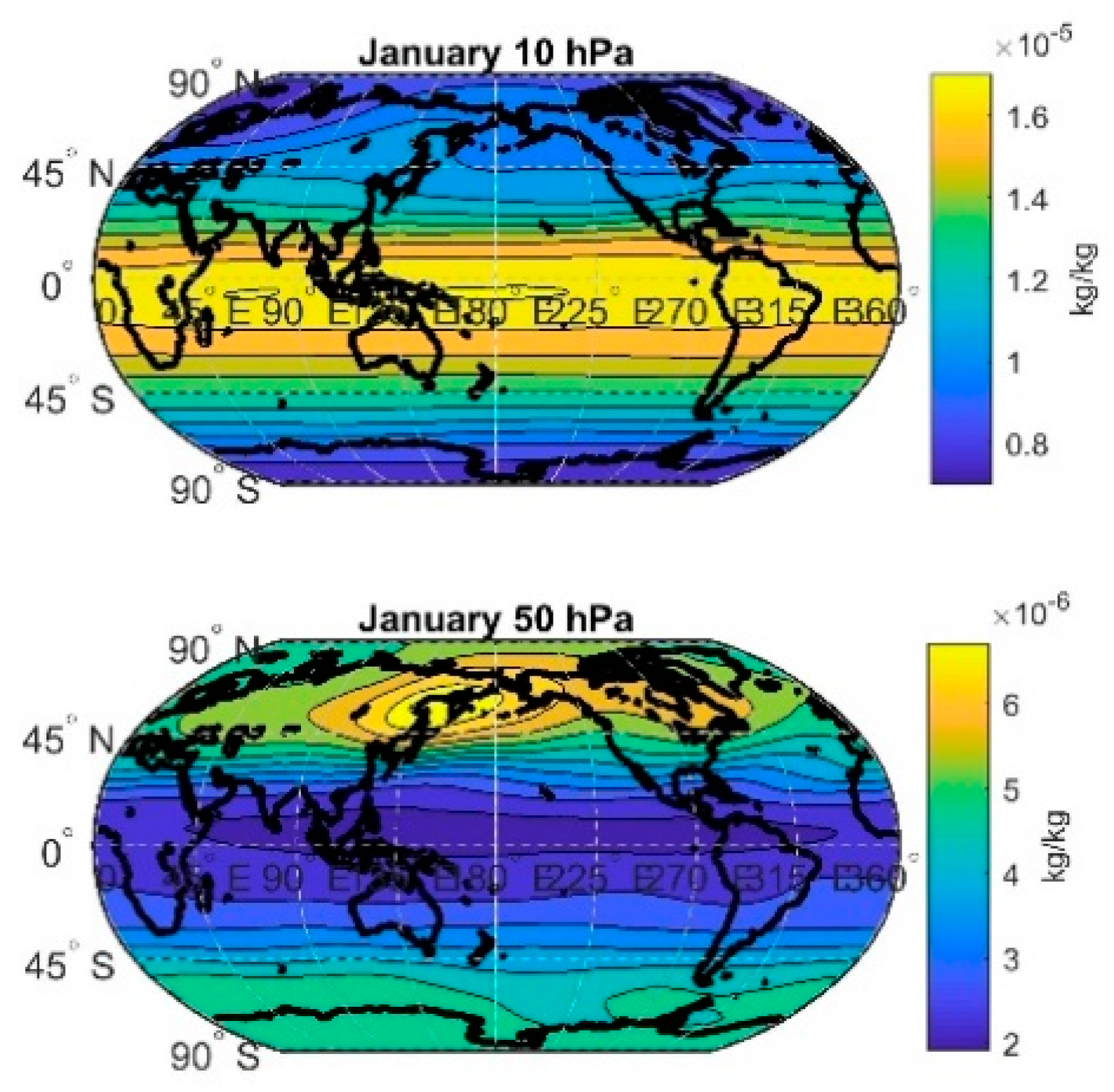
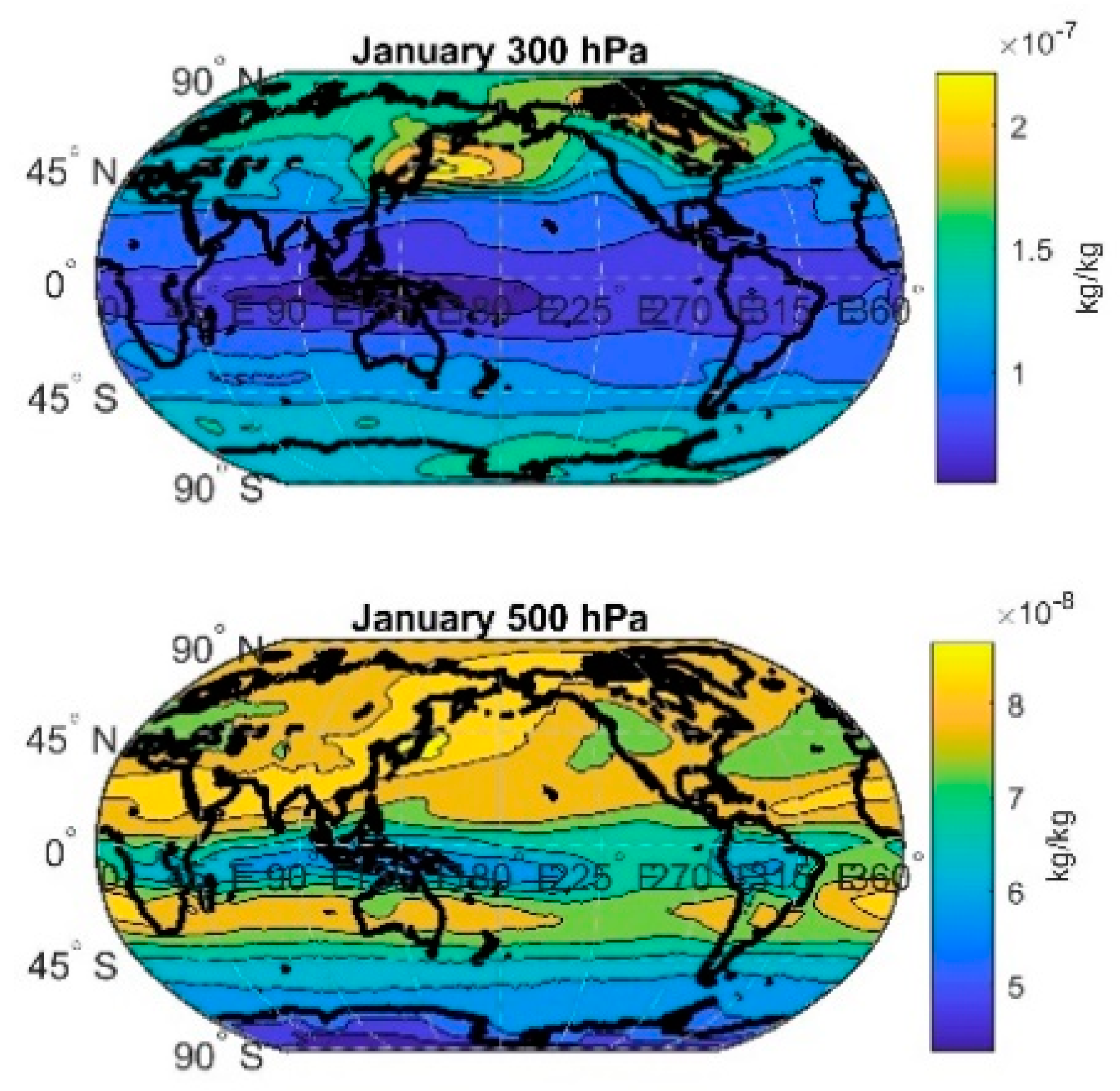
3.1. Patterns of Ozone Concentration

In Figure 1, one can see the map of ozone concentration at 0.1 hPa (upper panel) and at 0.5 hPa (lower panel). In the uppermost model layer, we see the strange pattern of the ozone concentration, which cannot be considered as real. At 0.5 hPa, this strange pattern was also present, but we also see the maximum in ozone concentration above the Aleutian Islands. At 1 hPa in January (Figure 2 upper panel), the strange unrealistic pattern ceased, but the maximum in the ozone concentration appeared over the Aleutian Islands. In July (Figure 2 lower panel), this maximum was situated in the subpolar latitudes of the Southern Hemisphere. At 2 hPa, this maximum was weaker and at 3 hPa disappeared. In the upper stratosphere (Figure 3 upper panel), we observed the equatorial maximum and the polar minimum of ozone concentration. In this layer, the solar radiation is the main factor that drives the ozone concentration. In the lower stratosphere (Figure 3 lower panel), the maximal concentration of ozone was seen in the high latitudes and the minimal one over the equator, which is given by the Brewer–Dobson circulation. The lower stratospheric maximum was persistent in the upper troposphere (Figure 4 upper panel). At 500 hPa (Figure 4 lower panel), this tropospheric maximum disappeared, and we observed maximal ozone concentration over the polluted areas of China and the United States of America. So, we found several ozone concentration patterns from 500 hPa up to the top of the model: tropospheric pattern, lower stratospheric, middle stratospheric pattern, maximum pattern, and strange pattern in the uppermost model layers. The pressure ranges in which these patterns occurred are given in Table 1. The strange pattern occurred above 0.5 hPa. The pattern with a maximum above the subpolar latitudes was seen from 0.7 hPa down to 2 (3) hPa. From October to March, this maximum was situated in the Northern Hemisphere, while from April to October in the Southern Hemisphere. In October, both maxima were present, but the northern maximum was much stronger than the southern one. Below this pattern, the upper stratospheric one with the maximum over the equator and the minimum over high latitudes of both hemispheres could be seen. The lower limit of this pattern was about 20 hPa in each month, and the upper limit was monthly dependant (from 7 to 3 hPa). The upper limit for the lower stratospheric pattern was 30 (40) hPa in each month, while this pattern had its lower edge deep in the troposphere (Figure 4 upper panel) in the Northern Hemisphere and from December to June also in the Southern Hemisphere. From July to November, we saw a secondary ozone concentration maximum also in the subpolar latitudes of the Southern Hemisphere, which is given by the fact the ozone hole starts to form in polar latitudes and so this maximum appeared as a consequence of this formation. If the ozone-destroying reactions did not act, one could expect a higher concentration of ozone in the polar latitudes of the Southern Hemisphere, and so no subpolar maximum occurs.

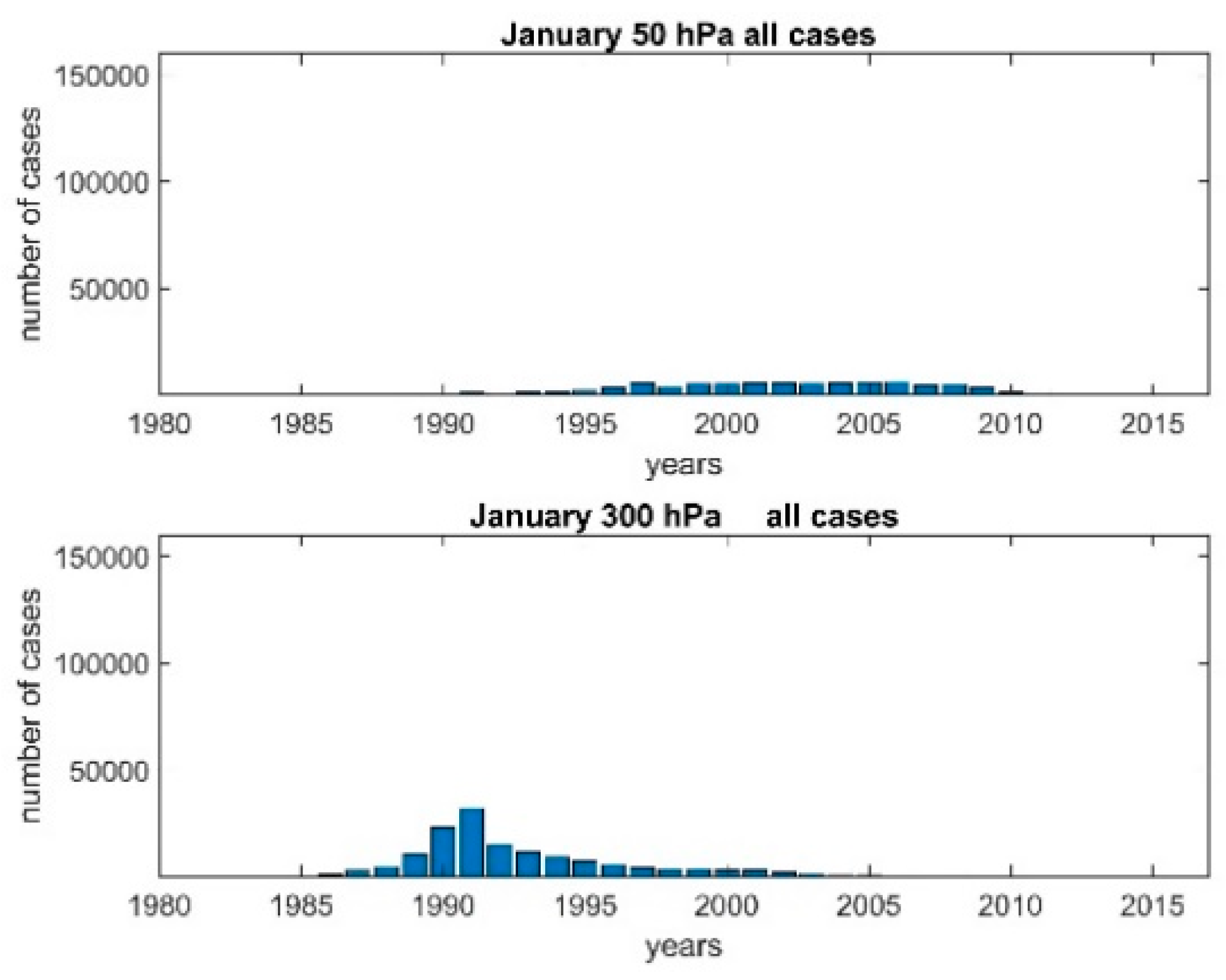
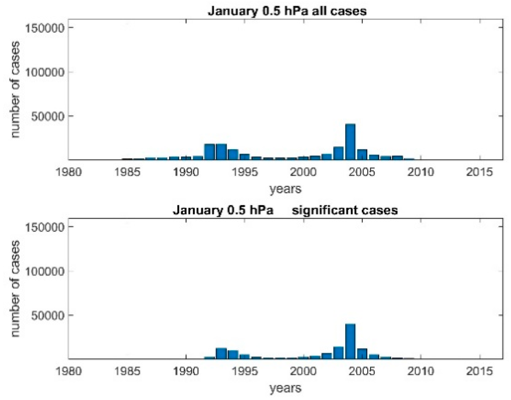
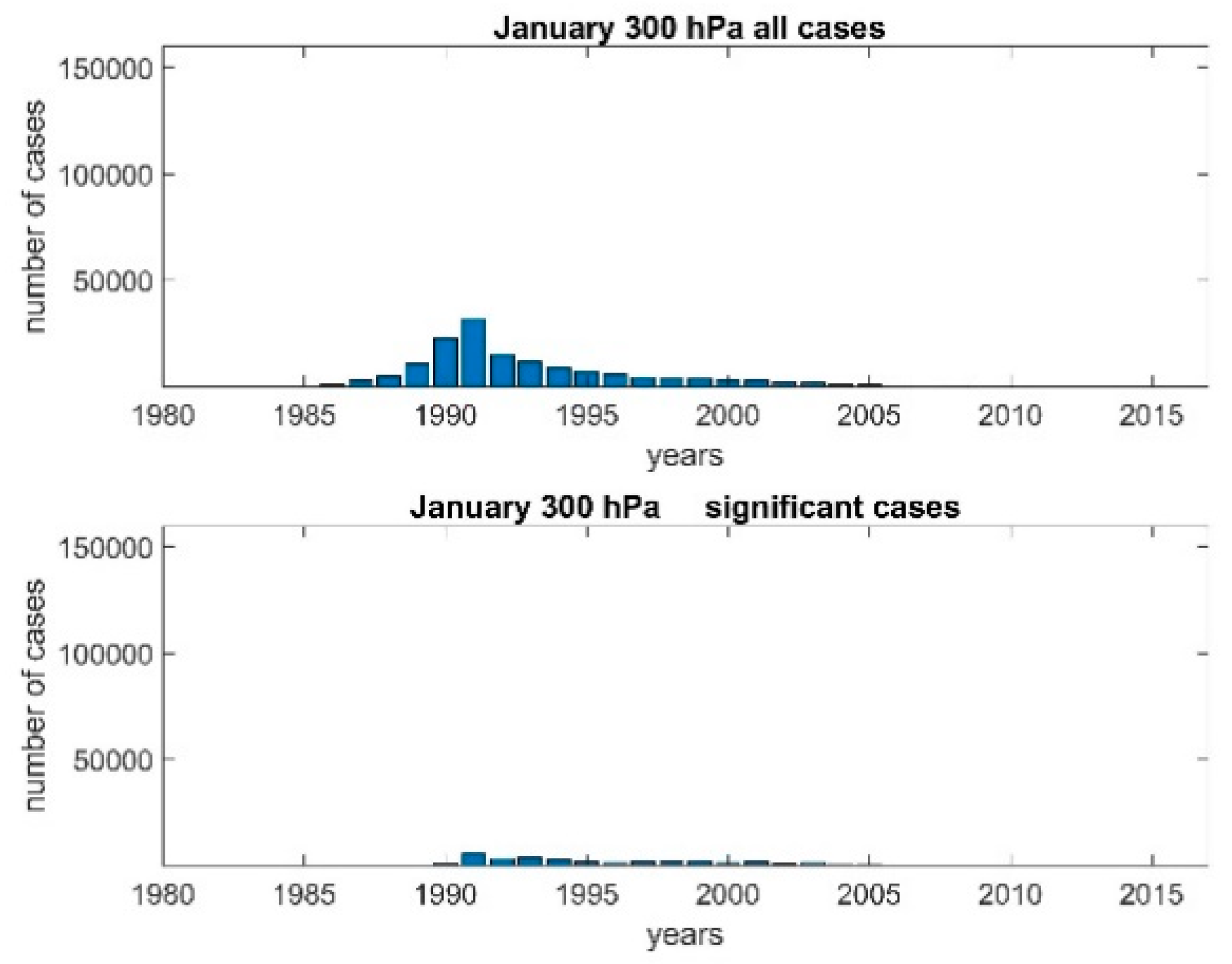
3.2. Temporal Occurrence of Discontinuities

Now we deal with the temporal occurrence of discontinuities in the MERRA 2 ozone data. When we look at Table 2, we see in the uppermost model layer in each month the unimodal temporal distribution with a maximum in 1993 (U93 Figure 5—upper panel for January). Going down this unimodal distribution change, the bimodal one with the main maximum was observed in 1993, and the secondary maximum was observed in 2004(B93,04). In lower layers, the bimodal distribution with the main maximum in 2004 and the secondary one in 1993 (B93,04) could be seen. This transformation ended at 1 hPa (Figure 5 lower panel for January), where we observed unimodal distribution again, but the maximum occurred in 2004 in each month. Below 2 hPa down to 200 hPa, we observed flat temporal distribution of discontinuities (F) with no sharp maximum (Figure 6 upper panel for January) in each month. In January, the upper distribution border lay in 5 hPa. Below 200 hPa, we again observed unimodal temporal distribution with a maximum about the early 1990s (U93T, Figure 6—lower panel for January), but this distribution was broader than distribution U93 in the upper model layers. When we observed the unimodal distribution of all discontinuities, the distribution of the significant ones must be similar. In the case of bimodal distribution, the situation was different. We could observe the bimodal distribution of all discontinuities, but the distribution of their significant counterparts can be unimodal. This was the case of bimodal distributions from 0.4 hPa and 0.5 hPa when we observed the bimodal distribution of all discontinuities, but the 1993 maximum was formed predominantly by the insignificant ones, and the 2004 maximum consisted predominantly of the significant discontinuities (Figure 7). Thus the distribution of the significant discontinuities in these cases was bimodal, but the maximum in 2004 was much stronger than that in 1993. Similarly, in the troposphere, the distribution U93T was seen only for all discontinuities, but for the significant ones, we observed nearly flat distribution due to the fact the 1993 maximum consisted predominantly of the insignificant discontinuities (Figure 8).

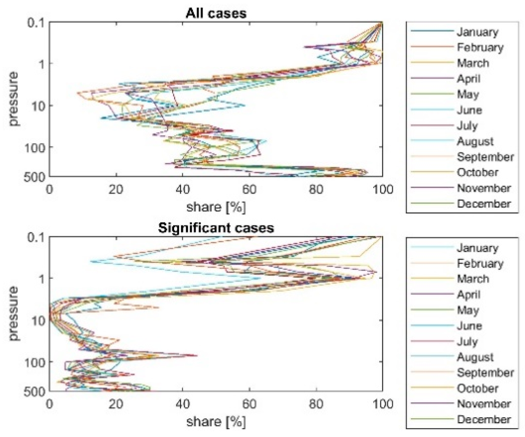
3.3. Vertical Profile of the Discontinuities Occurrence

In Figure 9 (upper panel), we see the vertical profile of the percentage occurrence of all discontinuities. One hundred percent means that the discontinuity occurred in each grid point (207,936 points), and 0% means there were no discontinuities in time series over the globe. The vertical profile pattern was similar in each month. In the uppermost model layer at each grid, the discontinuity occurred. Going down, the share of all discontinuities (Figure 9 upper panel) declined to 0.7 hPa. In 1 hPa, we observed their local maximum. Below this layer, the number of discontinuities declined to about 10 hPa, where we observed local occurrence minimum. From 10 hPa down to 200 hPa, the discontinuities occurred in 40%–60% of all grids. In the troposphere, the share of all discontinuities increased.
The vertical profiles of the significant discontinuities were similar (Figure 9 lower panel), but there were some interesting features in them. The local minimum about 0.7 hPa was much deeper than in the case of all discontinuities. The number of significant discontinuities was nearly zero about 10 hPa, and the tropospheric maximum, which was seen in the case of all discontinuities, was not present for the significant ones. With the increasing difference between the percentage of all discontinuities and the percentage of the significant ones, the share of significant discontinuities decreased.

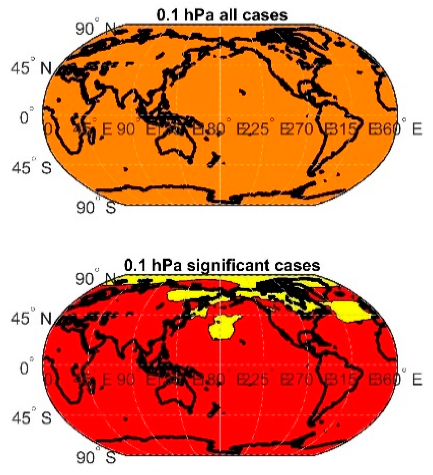
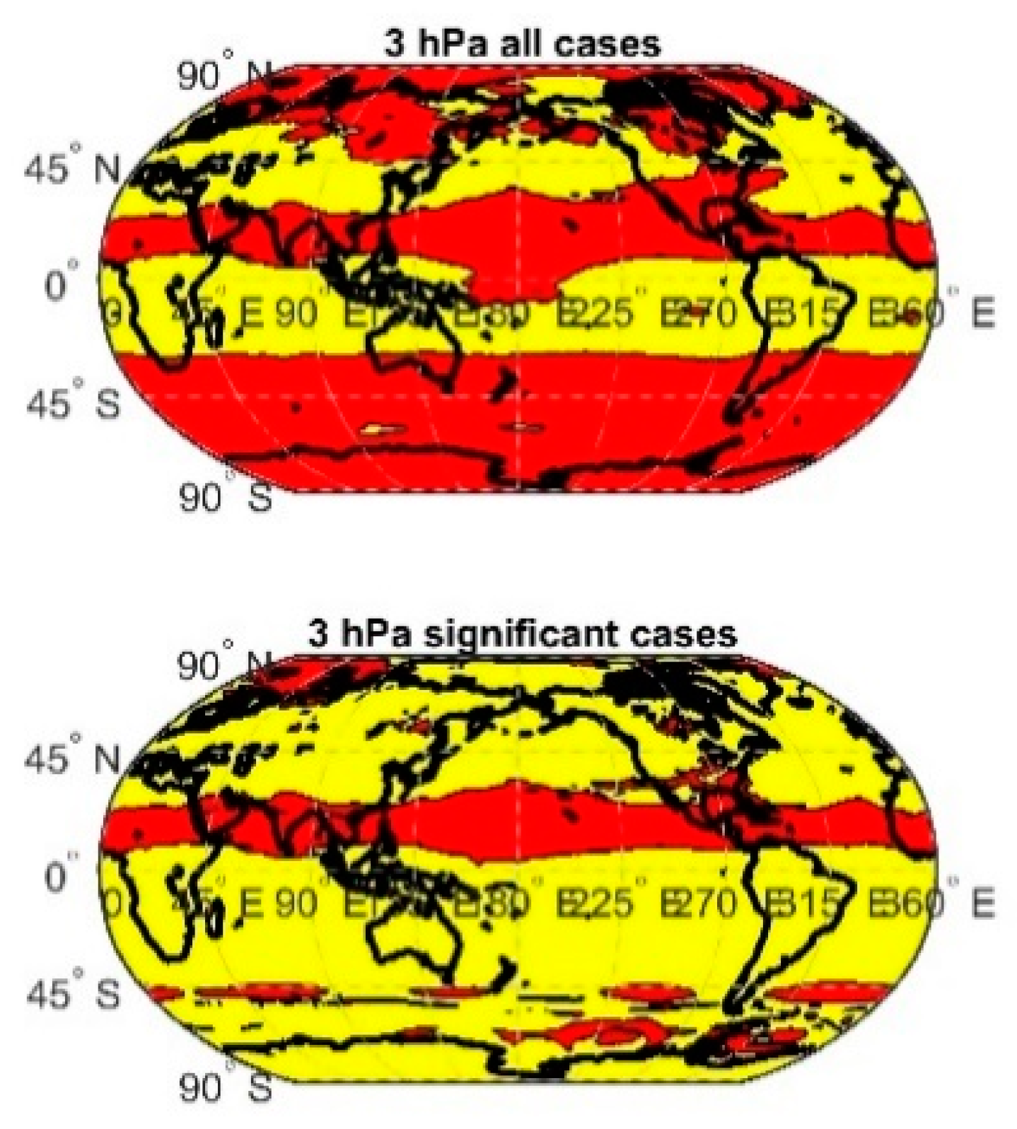
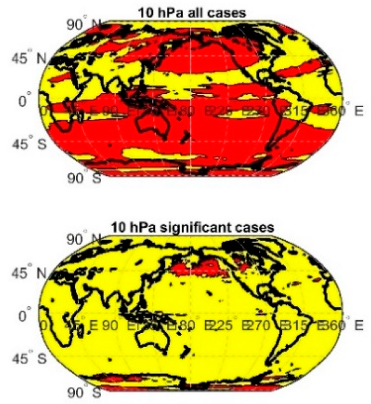
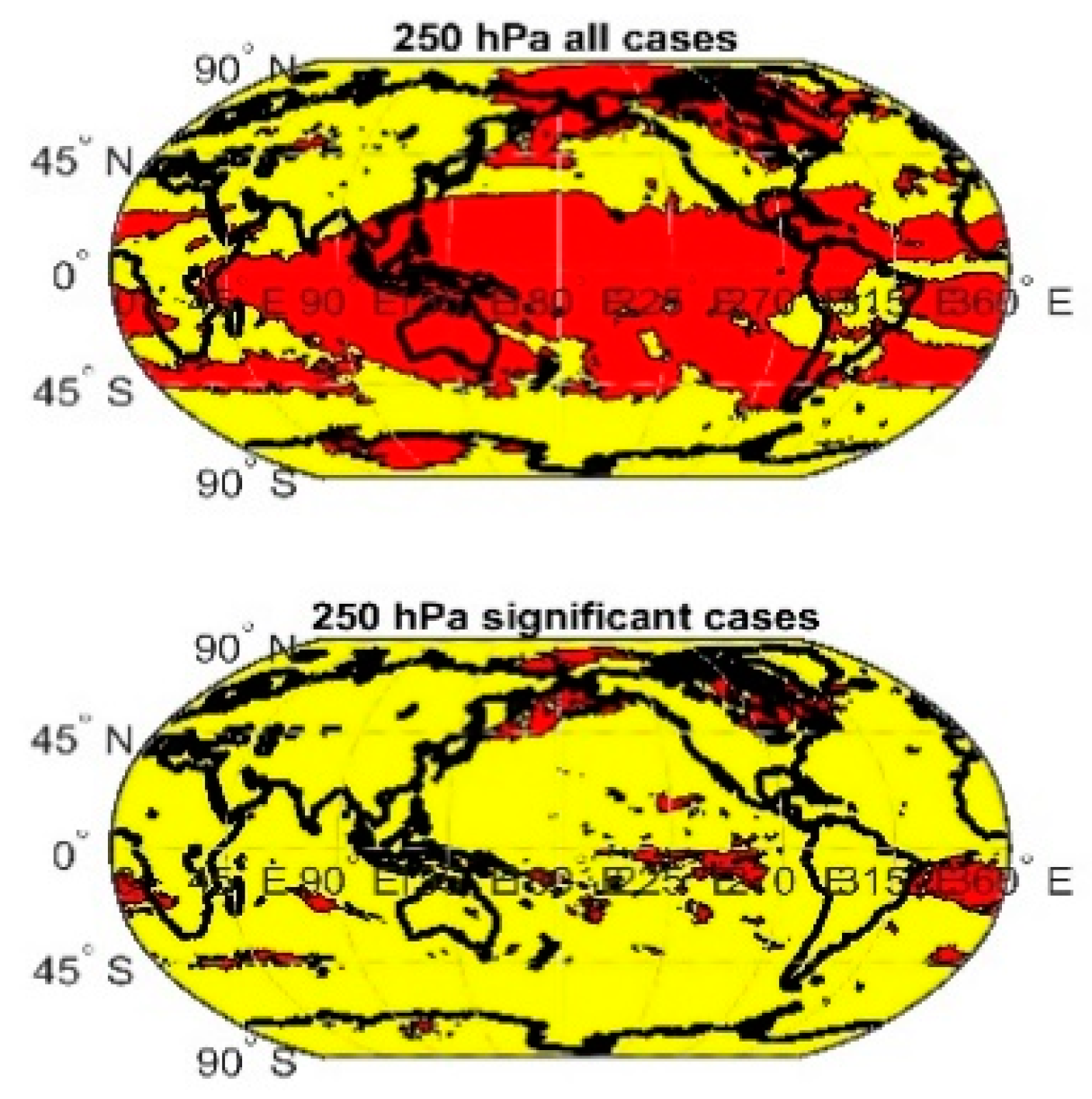
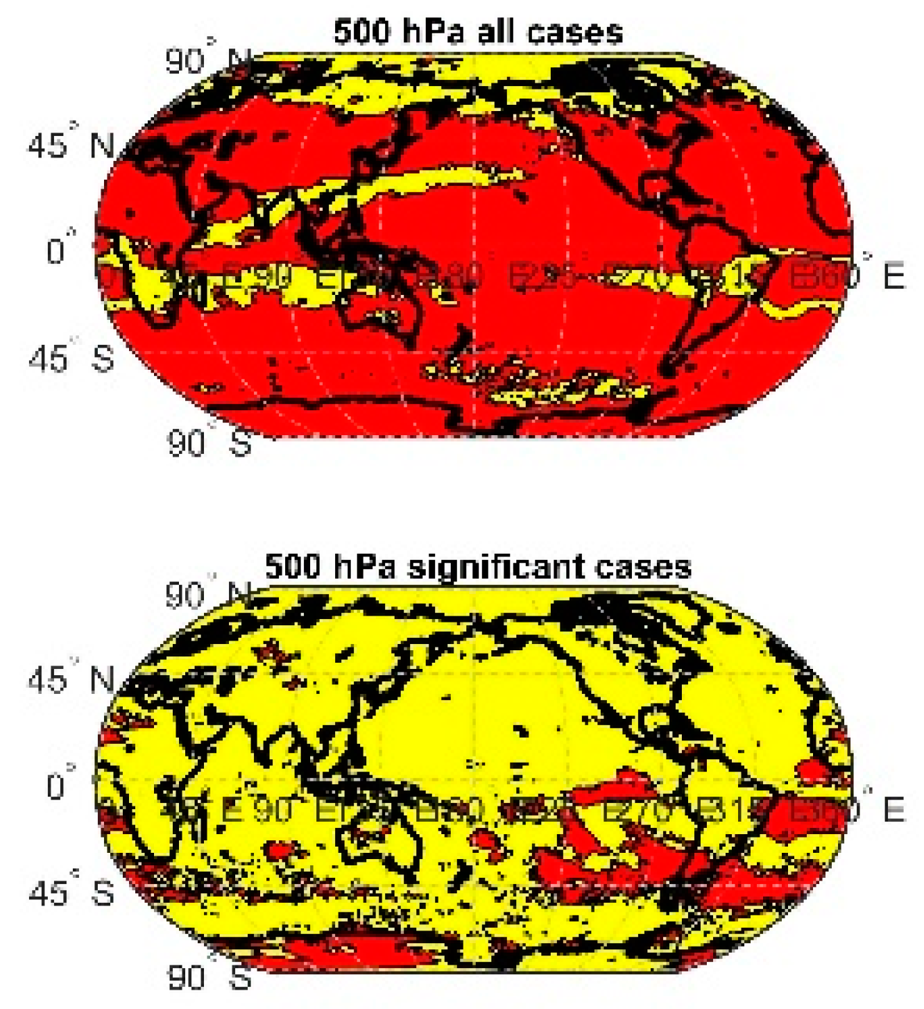
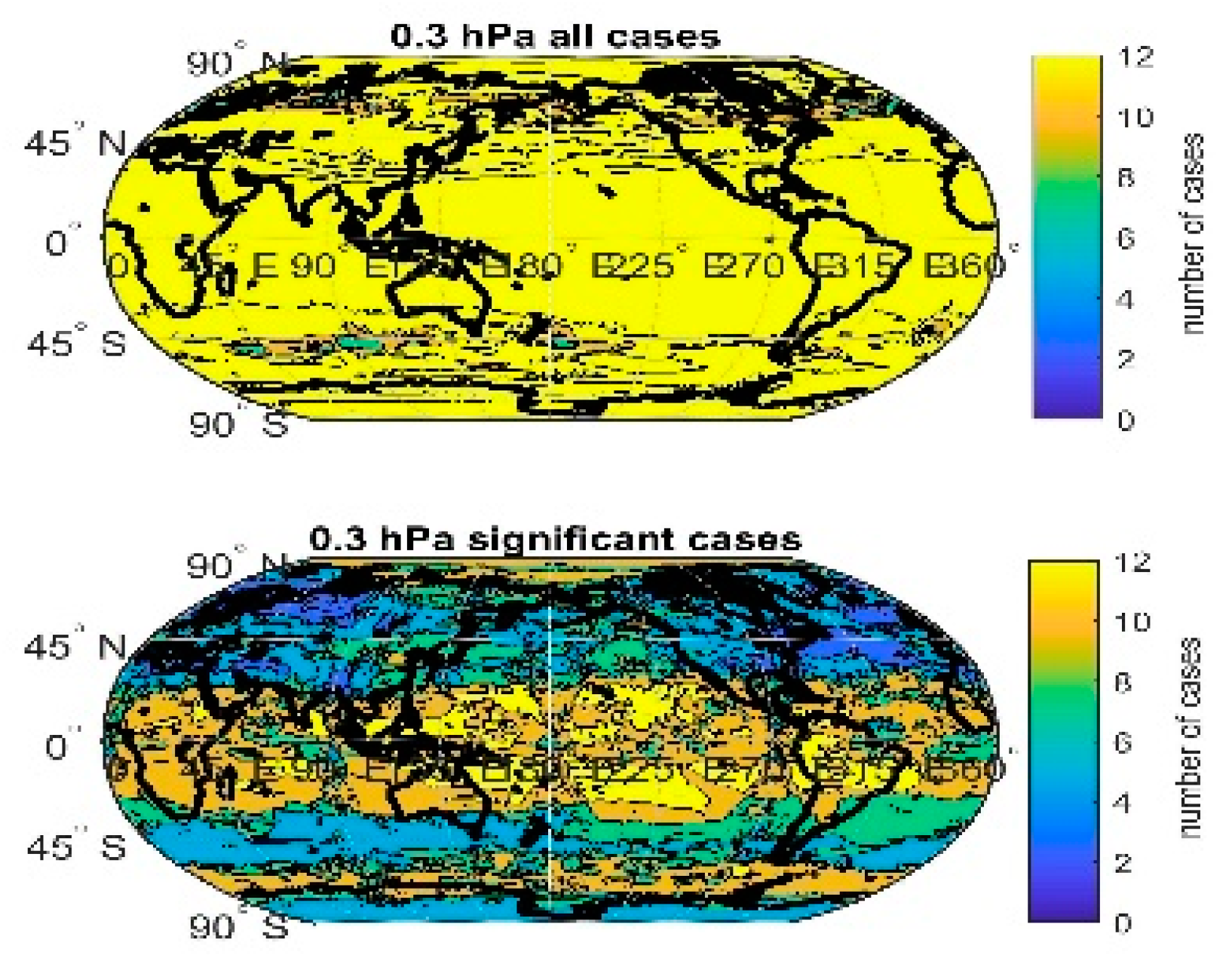
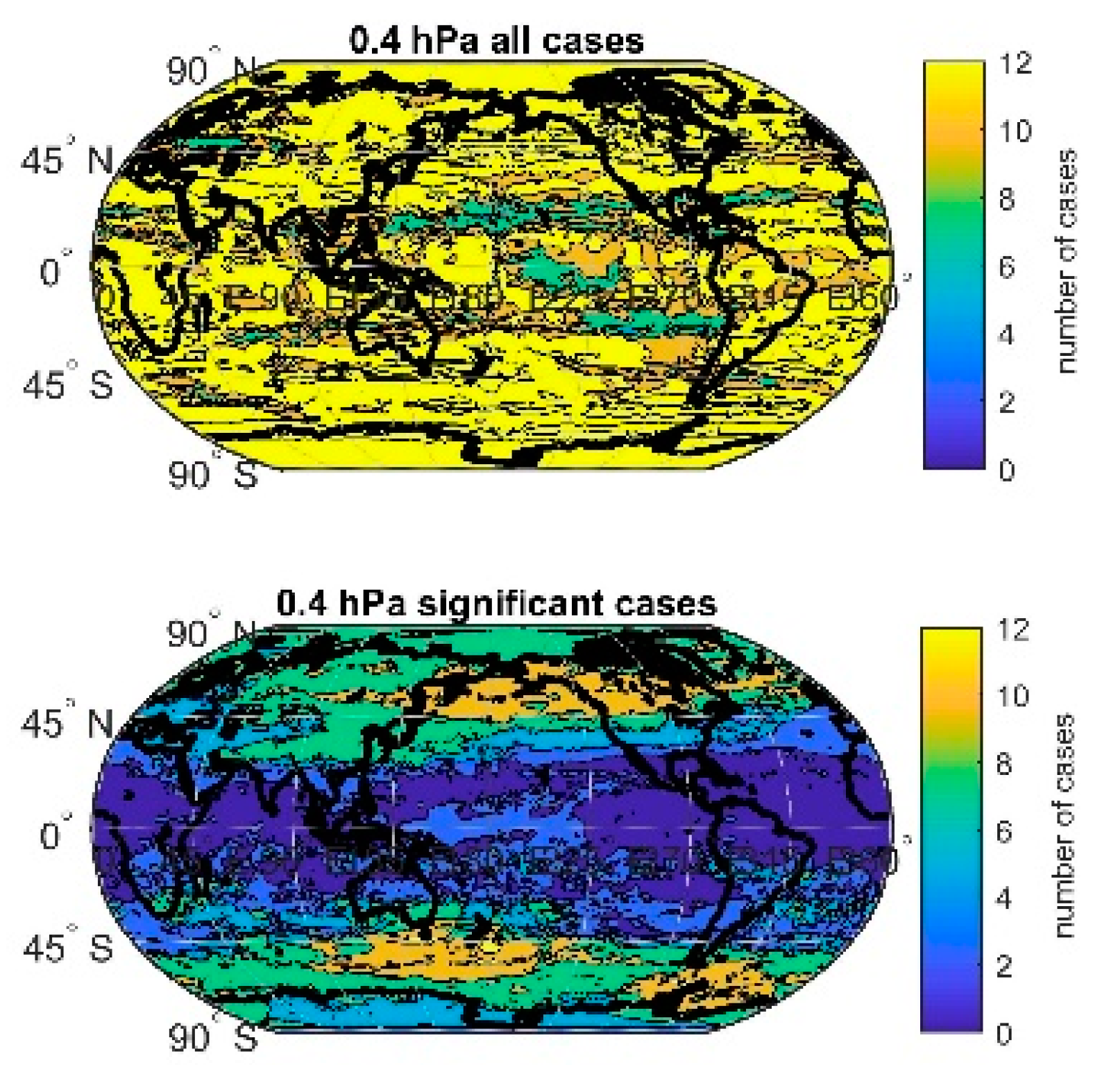
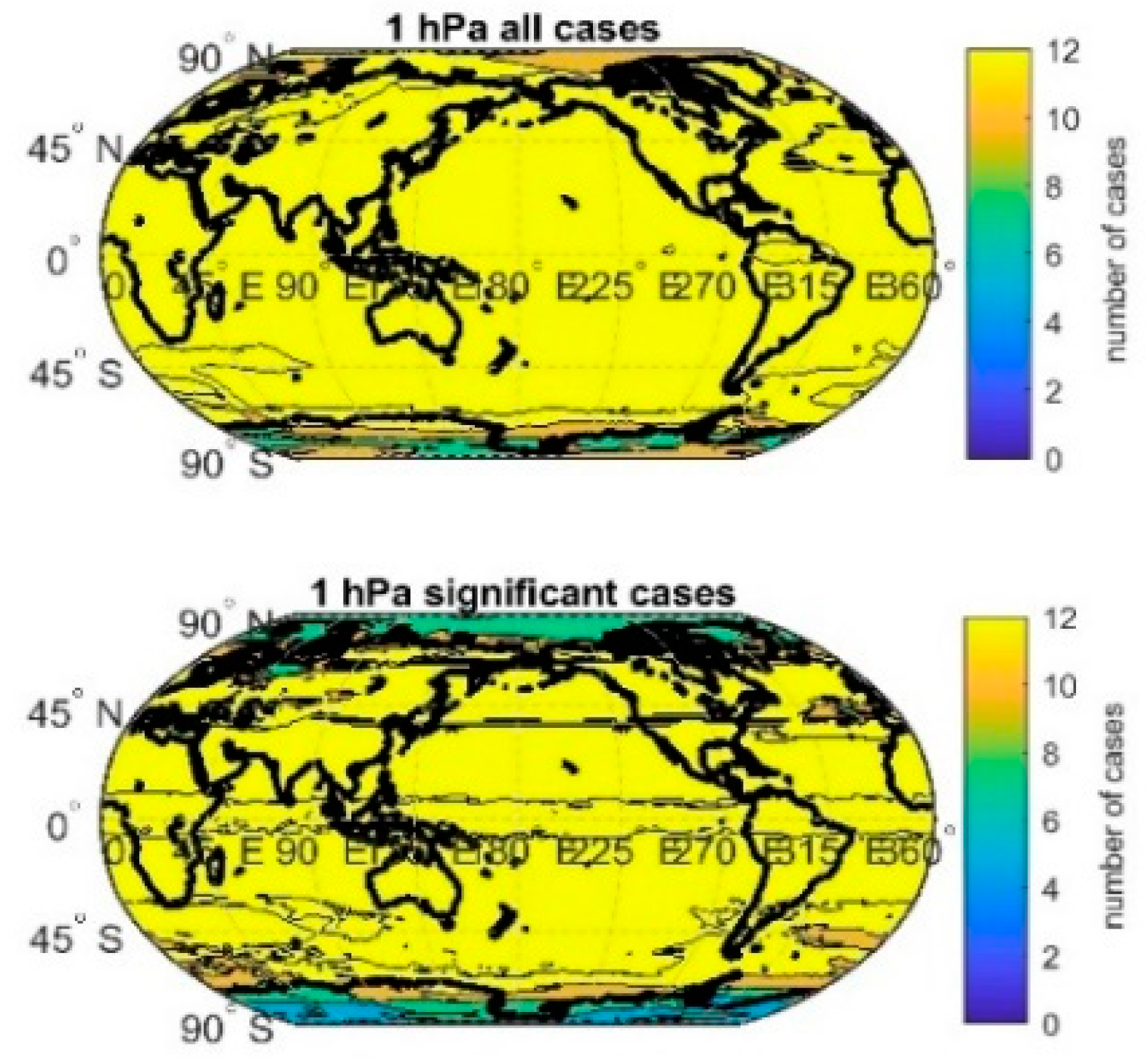
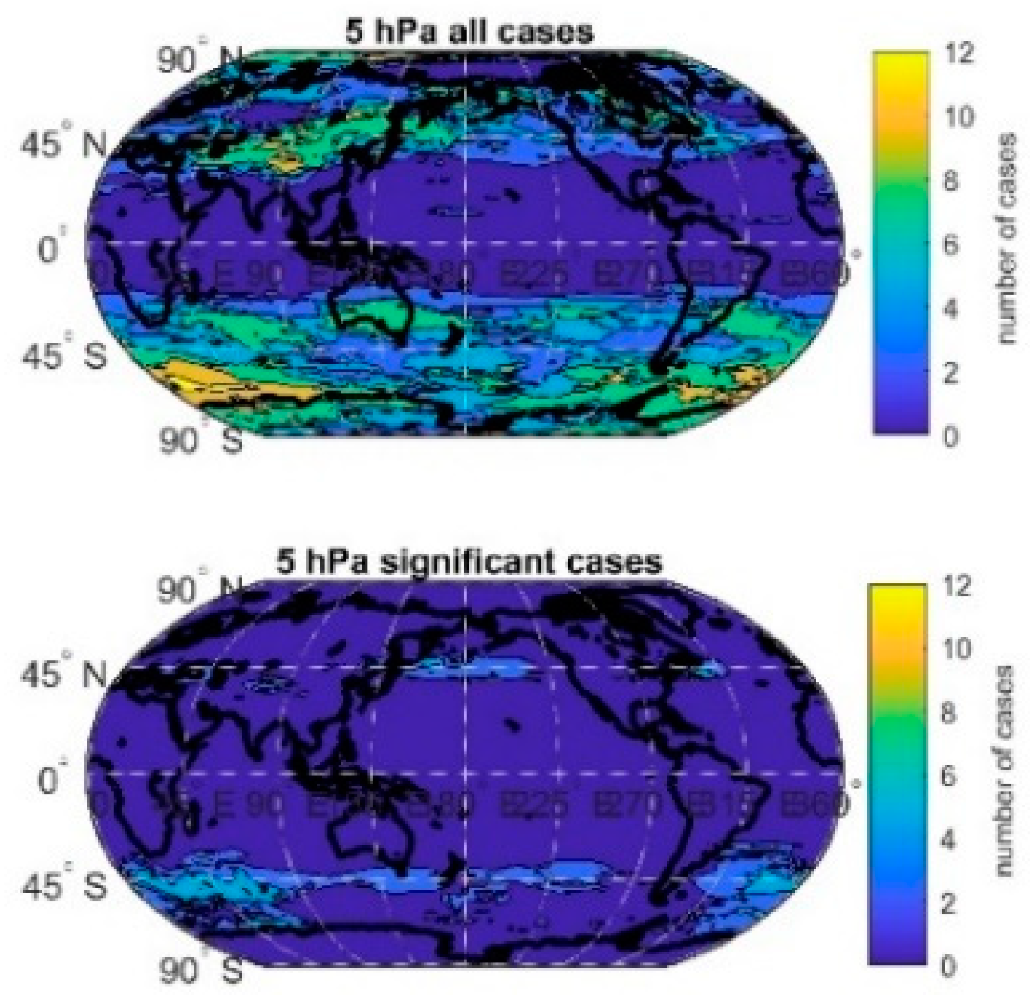
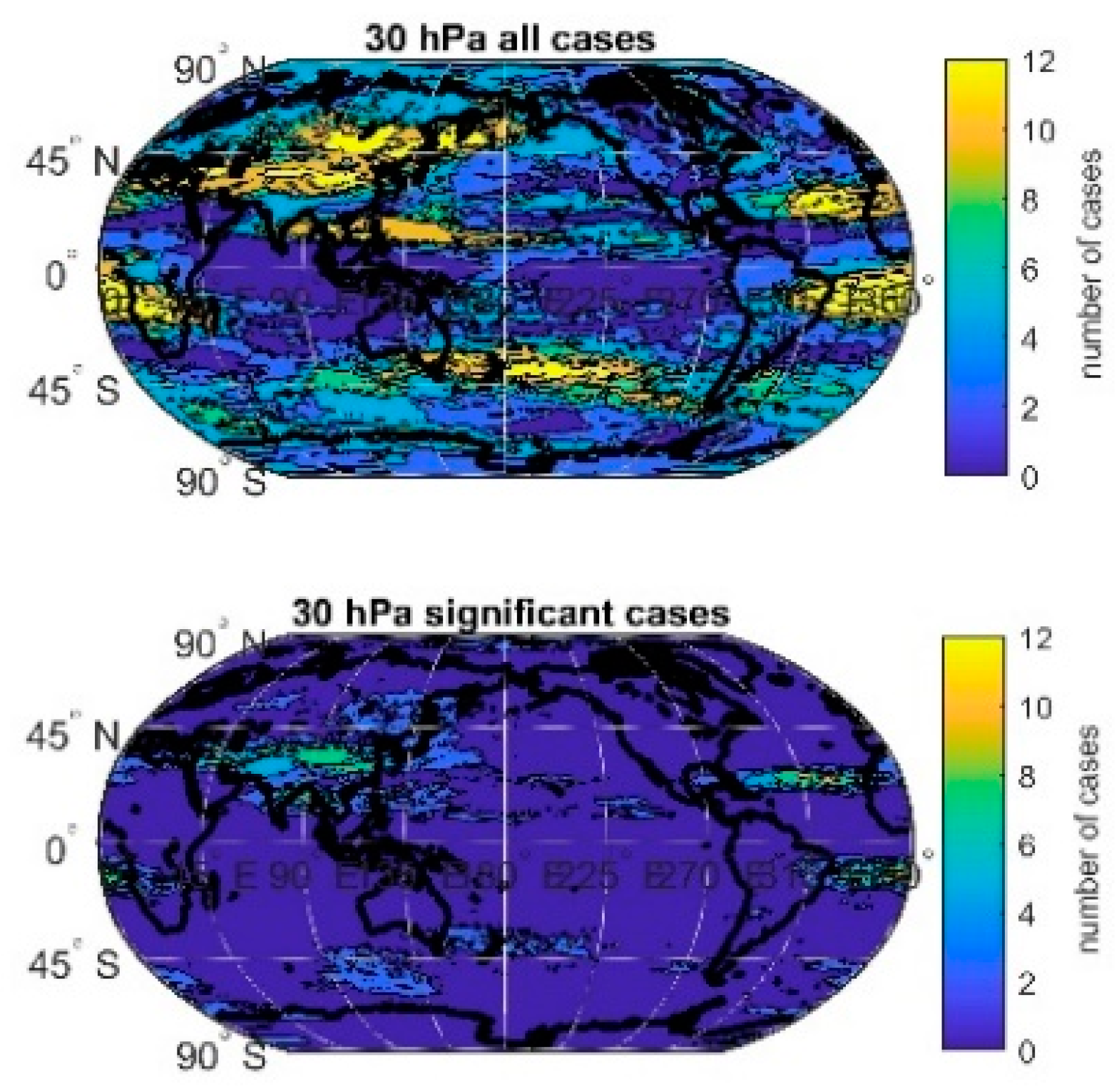
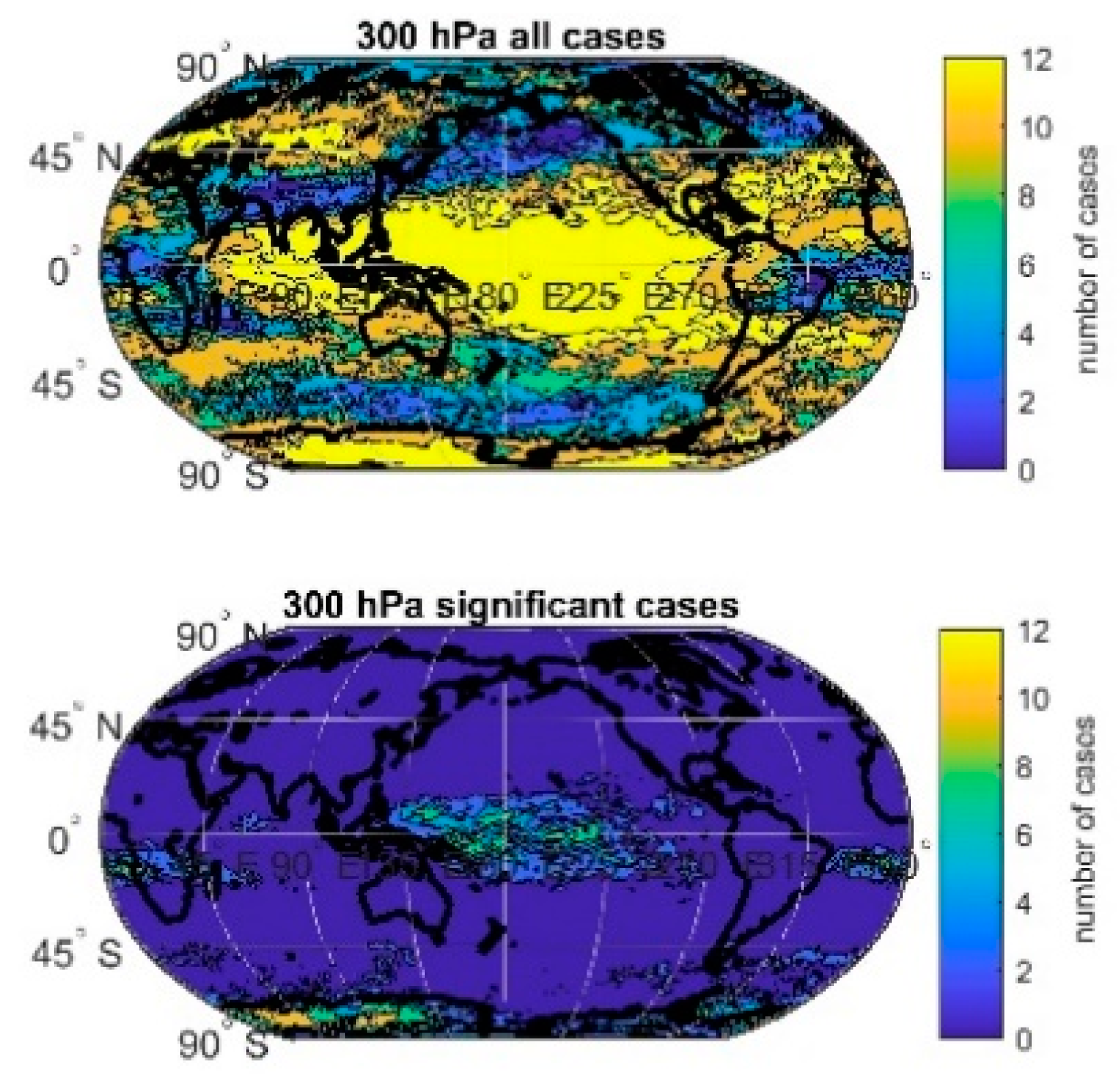
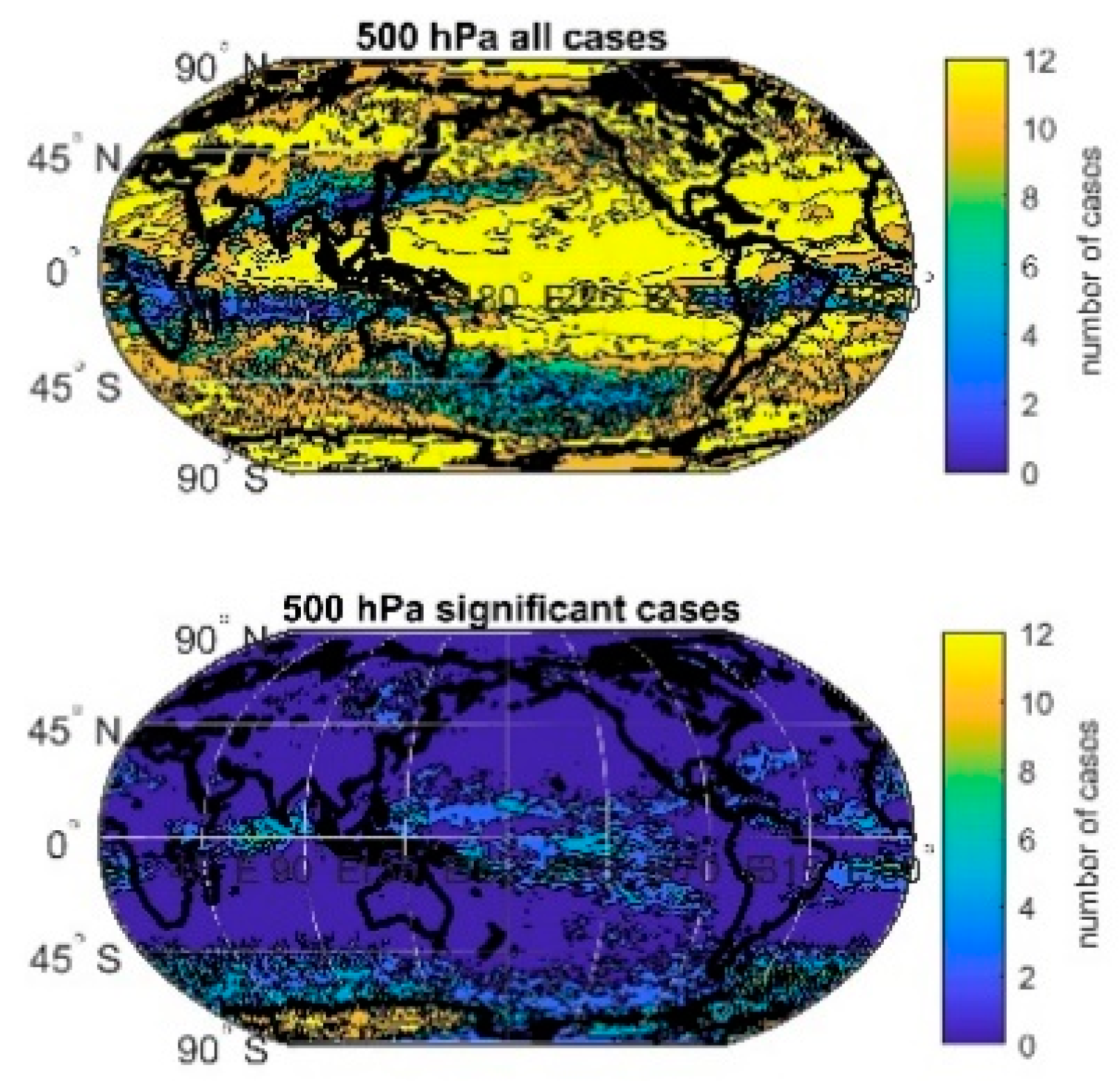
3.4. Spatial Occurrence of Discontinuities

Now we deal with the spatial occurrence of discontinuities over the globe. We present the results for January, but the results for other months were similar. Figure 10 (upper panel) shows the geographical distribution of all discontinuities at 0.1 hPa, and in the lower panel, the distribution of the significant ones is displayed. In this layer, there were discontinuities in all grids (orange colour in the upper panel of Figure 10), and their reduction for the significant ones was small. At 3hPa (Figure 11), the situation was different. The number of all discontinuities (upper panel) was smaller, and the number of their significant counterparts (lower panel) was strongly reduced. From 5 hPa down to 250 hPa, the number of significant and insignificant discontinuities were relatively low, and at these layers, almost there were no significant discontinuities (Figure 12 and Figure 13). From 300 hPa down to 500 hPa (Figure 14), the number of all discontinuities was very high, but the number of significant ones was low.
Now we search geographical areas where the discontinuities occur more often. This analysis will be done separately for all and significant discontinuities. At each layer and each grid, we computed for all months the sum of cases when we observed discontinuity in a certain grid. When the sum equals 12, it means that in this grid, the discontinuity was observed in each month. On the other hand, when the sum equals 0, it means there was no discontinuity in this grid in every month. The higher the sum, the more frequent occurrence of discontinuities was seen in this grid. At the uppermost model layers, the spatial distribution of the sum was layer-dependant (from 0.1 hPa down to 1 hPa). This can be illustrated in Figure 15 and Figure 16, where in the case of the insignificant discontinuities (lower panel) we observed at 0.3 hPa, a higher sum in the tropics than in the middle latitudes, but at 0.4 hPa (one layer below), the opposite was true. We observed a decrease in the sum from 1 hPa (Figure 17) down to 5 hPa (Figure 18) due to lower numbers of discontinuities. From 5 hPa down to 250 hPa, this sum for all and the significant discontinuities was relatively low, because the occurrence of discontinuities was rare. (Figure 19). In the troposphere (300 hPa Figure 20), we observed the increase in this sum, especially over the Pacific, in the case of all discontinuities. This sum was relatively low for the significant ones. This was caused by the vertical profile of discontinuity occurrence in the troposphere. From 300 hPa down to 500 hPa (Figure 21), the sum was high, but there were regions where this sum was much lower (over Africa and the Indian Ocean, over China, and over South America and the South Atlantic).

4. Discussion

When we look at the ozone concentration patterns at the uppermost model layers, we see the strange patterns down to 0.5 hPa (Figure 1 and Figure 2). According to our opinion, this is caused by the model itself, and these patterns are not real. So these layers are not suitable for trend analyses. The other groups of patterns are the ones with maximal concentration over the subpolar latitudes (from 0.7 to 2 hPa) of the winter hemisphere. It is very hard to explain this behaviour, because one can expect the main influence of solar activity to ozone at these heights, and in winter, there is very little solar radiation at the latitudes of maximum occurrence. In addition, at these heights, the ozone concentration is under the control of photochemistry, and the Brewer–Dobson circulation cannot act on them strongly. So one possible explanation is again the internal model variability, and the exploitation of these layers in trend analyses is problematic. Below these heights, the patterns with equatorial maximum and polar minimum were observed (from 3 down to 10 hPa). This is caused by the direct influence of solar radiation on ozone formation, which maximizes ozone in low latitude, and the Brewer–Dobson circulation is weak at these levels [24]. This upper stratospheric pattern can be explained by the theory, so in these heights, MERRA 2 gives reasonable results. From 30 hPa down to the tropopause, the maximal concentration was seen over high latitudes of both hemispheres and the minimal one over the equator. This is caused by the Brewer–Dobson circulation, which transports ozone rich air to high latitudes [25,26]. It is interesting these patterns persist deep into the troposphere, especially in the Northern Hemisphere, which may be caused by stratosphere–troposphere exchange in the vicinity of the Aleutian low.
The other topic of this paper, which is worth discussing, is the temporal occurrence of discontinuities in the period 1980–2017. In the uppermost model layer, the maximum of their occurrence was seen in 1993. One of the explanations of 1993 maximum is the Pinatubo eruption in 1991, but this maximum occurred only in the uppermost model layers. [27] found the enhanced wave activity in the two winters just after the Pinatubo eruption in similar heights. Thus the effect of the Pinatubo eruption may be real in the uppermost model layers. Going down this maximum disappeared, and the new one set up in 2004, and it was strongest at 1 hPa. This maximum can be clearly explained by the transition from SBUV to EOS Aura data in 2004 [12,28]. Below this layer, the flat temporal distribution of discontinuities was seen down to the troposphere, so no maximum in 2004 was observed. We can explain this fact by the following reasons. We can speculate the Pettitt test was either not suitable for this analysis, or the discontinuities in 2004 were not the most important in time series. The Pettitt test is widely used in atmospheric research, so we have no reason why this test does not work well for MERRA 2 ozone concentration data. If the 2004 discontinuities were not so huge, this fact could open the possibility of using MERRA 2 ozone data in trend analysis. The decision regarding these two hypotheses will be a matter of future research. In the troposphere, we observed wide maximum again in 1993, but not in 2004. In future work, we shall look at the wave activity in the upper troposphere and search its connection with the discontinuities occurrence peak in 1993.
Shangguan et al. [12] also detected discontinuities in 2015 when version 4.2 of the Microwave Limb Sounder (MLS) ozone data were used instead of version 2.2 and in 1998 when the Advanced TIROS (The Television Infrared Observation Satellite) Operational Vertical Sounder (ATOVS) was launched. In our paper, these discontinuities were not detected due to these reasons: We used data in the period of 1980–2017, so the year 2015 is at the edge of the series, and the Pettitt test could not capture this year. In each grid, we took into account only one main discontinuity, so the year 1998 could not be the main discontinuity, and thus, we did not notice it.
When we look at the vertical profile of discontinuity occurrence, we see the two main areas: the uppermost model layers and the tropospheric layers. From about 2 hPa down to the troposphere, we observed fewer discontinuities. High occurrence of discontinuities in the lowermost stratosphere and the upper troposphere can be explained by the lower quality of SBUV ozone data in these layers [29]. The share of the significant discontinuities was high in the upper model layer, while this share was low in the troposphere. The less number of (significant) discontinuities, the better for trend analysis.
We can conclude that due to ozone concentration patterns and the occurrence of discontinuities, the layers above 4 hPa are not suitable for trend analyses in MERRA 2. Below 4 hPa, the MERRA 2 gives explainable results expected from the theory, which also promotes using these data in the trend analysis. According to our results, the transition from SBUV to EOS Aura data does not have a major impact on discontinuity occurrence at these layers. The worst condition for trend analyses was the occurrence of the significant discontinuities in time series, and the share of grids with them was relatively low below 4 hPa. The better situation was the existence of discontinuities, which were not significant. Their number was higher than the significant ones. The grids with no discontinuities were not rare in the MERRA 2 ozone concentration data.
We must also deal with the possibility of the occurrence of discontinuities with natural origin. They must be included in trend analysis because they are real. It is very difficult to distinguish between artificial and real discontinuities because the real ones occur when there is some natural change in the atmosphere. We must consider the possibility of atmospheric changes connected to the change in ozone content and with increasing concentration of CO2. Sudden water vapour drops in the stratosphere around 2000. In ref [30] can also be the manifestation of the changes in the atmospheric behaviour.
Almost all the modern reanalyses had a temporal discontinuity in 1998 when the ATOVS observations became available, and the reanalyses either switched immediately or transitioned from the TIROS Operational Vertical Sounder (TOVS) to the ATOVS over several years. These discontinuities were not consistent in each latitude or pressure level. The disagreement in the polar latitudes of the southern Hemisphere extended lower into the stratosphere than in the northern hemispheric ones. The zonal wind variance was smaller than the temperature variance in the polar latitudes, but had a similar temporal difference between the TOVS and ATOVS time periods. For the tropics, the zonal wind variance is much larger than in the polar regions, and the disagreement between the semi-annual oscillation (SAO) and QBO zonal winds is quite large. Thus, improving equatorial winds in future reanalyses is an important goal. MERRA 2 reanalysis also showed discontinuities in 2004 when MLS observations were included. The disagreement was evident mainly for temperature or zonal wind. More details about discontinuities in reanalyses can be found in ref [31].

5. Conclusions

The main achievements concerning the ability to utilize the MERRA 2 ozone data for trend studies based on the Pettitt test results and on the analyses of monthly averages are the following:
  • The data above 4 hPa are not suitable for the trend analyses due to occurrence of patterns of the average ozone concentration which cannot be explained by theory and due to the frequent occurrence of the significant discontinuities
  • Below 4 hPa, the number of discontinuities is smaller, and they are mostly insignificant.
  • In the troposphere, the number of discontinuities is higher than in the stratosphere, but they are mostly insignificant.
  • The transition from SBUV to EOS Aura data in 2004 does not have a strong influence on discontinuities occurrence below 4 hPa.
  • According to our results, the MERRA 2 ozone concentration data are suitable for trend analyses below 4 hPa with caution.

Author Contributions

This paper was done in close collaboration of the authors, but substantial part of the works was done by P.K.

Funding

Support by the Grant Agency of the Czech Republic via Grant 18-01625S is acknowledged.

Conflicts of Interest

The authors declare no conflict of interest.

References

  1. Farman, J.; Gardiner, B.; Shanklin, J. Large losses of total ozone in Antarctica reveal seasonal ClOx/NOx interaction. Nature 1985, 315, 207–210. [Google Scholar] [CrossRef]
  2. Solomon, S. Stratospheric ozone depletion: A review of concepts and history. Rev. Geophys. 1999, 37, 275–316. [Google Scholar] [CrossRef]
  3. WMO. Scientific Assessment of Ozone Depletion: 2014 Global Ozone Research and Monitoring Project Report; World Meteorological Organization: Geneva, Switzerland, 2014; p. 416. [Google Scholar]
  4. Harris, N.R.P.; Hassler, B.; Tummon, F.; Bodeker, G.E.; Hubert, D.; Petropavlovskikh, I.; Steinbrecht, W.; Anderson, J.; Bhartia, P.K.; Boone, C.D.; et al. Past changes in the vertical distribution of ozone—Part 3: Analysis and interpretation of trends. Atmos. Chem. Phys. 2015, 15, 9965–9982. [Google Scholar] [CrossRef] [Green Version]
  5. Eyring, V.; Cionni, I.; Bodeker, G.E.; Charlton-Perez, A.J.; Kinnison, D.E.; Scinocca, J.F.; Waugh, D.W.; Akiyoshi, H.; Bekki, S.; Chipperfield, M.P.; et al. Multi-model assessment of stratospheric ozone return dates and ozone recovery in CCMVal-2 models. Atmos. Chem. Phys. 2010, 10, 9451–9472. [Google Scholar] [CrossRef] [Green Version]
  6. Waugh, D.W.; Oman, L.; Kawa, S.R.; Stolarski, R.S.; Pawson, S.; Douglass, A.R.; Newman, P.A.; Nielsen, J.E. Impacts of climate change on stratospheric ozone recovery. Geophys. Res. Lett. 2009, 36, L03805. [Google Scholar] [CrossRef] [Green Version]
  7. McLandress, C.H.; Sheepherd, T.G. Simulated anthropogenic changes in the brewer-dobson circulation, including its extension to high latitudes. J. Clim. 2009, 22, 1516–1540. [Google Scholar] [CrossRef]
  8. Angell, J.K.; Melissa, F. Ground-based observations of the slowdown in ozone decline and onset of ozone increase. J. Geophys. Res. 2009, 114, D07303. [Google Scholar] [CrossRef] [Green Version]
  9. Krzyscin, J.W.; Borkowski, J.L. Variabilty of the total ozone trend over Europe for the period 1950–2004 derived from reconstructed data. Atmos. Chem. Phys. 2008, 8, 2847–2857. [Google Scholar] [CrossRef] [Green Version]
  10. Jones, A.; Urban, J.; Murtagh, D.P.; Eriksson, P.; Brohede, S.; Haley, C.; Degenstein, D.; Bourassa, A.; von Savigny, C.; Sonkaew, T.; et al. Evolution of stratospheric ozone and water vapour time series studied with satellite measurements. Atmos. Chem. Phys. 2009, 9, 6055–6075. [Google Scholar] [CrossRef] [Green Version]
  11. Bengtsson, L.; Hagemann, S.; Hodges, K.I. Can climate trends be calculated from reanalysis data? J. Geophys. Res. Atmos. 2004, 109, D11111. [Google Scholar] [CrossRef] [Green Version]
  12. Shangguan, M.; Wang, W.; Jin, S. Variability of temperature and ozone in the upper troposphere and lower stratosphere from multi-satellite observations and reanalysis data. Atmos. Chem. Phys. 2019, 19, 6659–6679. [Google Scholar] [CrossRef] [Green Version]
  13. Takacs, L.L.; Suárez, M.J.; Todling, R. Maintaining atmospheric mass and water balance in reanalyses. Q. J. Roy. Meteorol. Soc. 2016, 142, 1565–1573. [Google Scholar] [CrossRef] [PubMed] [Green Version]
  14. Molod, A.; Takacs, L.; Suarez, M.; Bacmeister, J. Development of the GEOS-5 atmospheric general circulation model: Evolution from MERRA to MERRA2. Geosci. Model Dev. 2015, 8, 1339–1356. [Google Scholar] [CrossRef] [Green Version]
  15. Coy, L.; Wargan, K.; Molod, A.M.; McCarty, W.R.; Pawson, S. Structure and dynamics of the quasi-biennial oscillation in MERRA-2. J. Clim. 2016, 29, 5339–5354. [Google Scholar] [CrossRef] [PubMed]
  16. Randles, C.A.; da Silva, A.M.; Buchard, V.; Darmenov, A.; Colarco, P.R.; Aquila, V.; Bian, H.; Nowottnick, E.P.; Pan, X.; Smirnov, A.; et al. The MERRA-2 aerosol assimilation, NASA Technical Report Series on Global Modeling and Data Assimilation, Volume 45; NASA/TM-2016-104606; NASA Goddard Space Flight Center: Greenbelt, MD, USA, 2016.
  17. Fujiwara, M.; Wright, J.S.; Manney, G.L.; Gray, L.J.; Anstey, J.; Birner, T.; Davis, S.; Gerber, E.P.; Harvey, V.L.; Hegglin, M.I.; et al. Introduction to the SPARC Reanalysis Intercomparison Project (S-RIP) and overview of the reanalysis systems. Atmos. Chem. Phys. 2017, 17, 1417–1452. [Google Scholar] [CrossRef] [Green Version]
  18. Gelaro, R.W.; McCarty, M.J.; Suárez, R.; Todling, A.; Molod, L.; Takacs, C.A.; Randles, A.; Darmenov, M.G.; Bosilovich, R.; Reichle, K.; et al. The modern-era retrospective analysis for research and applications, Version 2 (MERRA-2). J. Clim. 2017, 30, 5419–5454. [Google Scholar] [CrossRef]
  19. Pettitt, A.N. A non-parametric approach to the change point detection. Appl. Statist. 1979, 28, 126–135. [Google Scholar] [CrossRef]
  20. Javari, M. Trend and homogeneity analysis of precipitation in Iran. Climate 2016, 4, 44. [Google Scholar] [CrossRef]
  21. Firat, M.; Dikbas, F.; Cem Koç, A.; Gungor, M. Missing data analysis and homogeneity test for Turkish precipitation series. Sadhana 2010, 35, 707–720. [Google Scholar] [CrossRef]
  22. Wijngaard, J.B.; Klein Tank, A.M.G.; Knnen, G.P. Homogeneity of 20th century European daily temperature and precipitation series. Int. J. Climatol. 2003, 23, 679–692. [Google Scholar] [CrossRef]
  23. Kruskal, W.H. Historical notes on the Wilcoxon unpaired two-sample test. J. Am. Stat. Assoc. 1957, 52, 356–360. [Google Scholar] [CrossRef]
  24. Dütsch, H.U. The ozone distribution in the atmosphere. Can. J. Chem. 1974, 52, 1491–1504. [Google Scholar] [CrossRef]
  25. Williams, R.S.; Hegglin, M.I.; Kerridge, B.J.; Jöckel, P.; Latter, B.G.; Plummer, D.A. Characterising the seasonal and geographical variability in tropospheric ozone, stratospheric influence and recent changes. Atmos. Chem. Phys. 2019, 19, 3589–3620. [Google Scholar] [CrossRef] [Green Version]
  26. Rowland, F.S. Stratospheric ozone depletion. Philos. Trans. R. Soc. Lond. B Biol. Sci. 2006, 361, 769–790. [Google Scholar] [CrossRef] [PubMed]
  27. Lastovicka, J.; Buresova, D.; Boska, J. Does the QBO and the Mt. Pinatubo eruption affect the gravity wave activity in the lower ionosphere? Studia Geophys. Geod. 1998, 42, 170–182. [Google Scholar] [CrossRef]
  28. Wargan, K.; Labow, G.; Frith, S.; Pawson, S.; Livesey, N.; Partyka, G. Evaluation of the ozone fields in NASA’s MERRA-2 reanalysis. J. Clim. 2017, 30, 2961–2988. [Google Scholar] [CrossRef] [PubMed] [Green Version]
  29. Bhartia, P.K.; McPeters, R.D.; Flynn, L.E.; Taylor, S.; Kramarova, N.A.; Frith, S.; Fisher, B.; DeLand, M. Solar Backscatter UV (SBUV) total ozone and profile algorithm. Atmos. Meas. Tech. 2013, 6, 2533–2548. [Google Scholar] [CrossRef] [Green Version]
  30. Brinkop, S.; Dameris, M.; Jöckel, P.; Garny, H.; Lossow, S.; Stiller, G. The millennium water vapour drop in chemistry-climate model simulations. Atmos. Chem. Phys. 2016, 16, 8125–8140. [Google Scholar] [CrossRef] [Green Version]
  31. Long, C.S.; Fujiwara, M.; Davis, S.; Mitchell, D.M.; Wright, C.J. Climatology and interannual variability of dynamic variables in multiple reanalyses evaluated by the SPARC Reanalysis Intercomparison Project (S-RIP). Atmos. Chem. Phys. 2017, 17, 14593–14629. [Google Scholar] [CrossRef] [Green Version]
Figure 1. Average ozone concentration (kg/kg) in January at 0.1 hPa (upper panel) and at 0.5 hPa (lower panel).
Atmosphere 10 00812 g001
Figure 2. The same as Figure 1, but for January at 1 hPa (upper panel) and for July at 1 hPa (lower panel).
Atmosphere 10 00812 g002
Figure 3. Average ozone concentration (kg/kg) in January at 10 hPa (upper panel) and at 50 hPa (lower panel).
Atmosphere 10 00812 g003
Figure 4. Average ozone concentration (kg/kg) in January at 300 hPa (upper panel) and at 500 hPa (lower panel).
Atmosphere 10 00812 g004
Figure 5. Temporal distribution of all discontinuities in January at 0.1 hPa (upper panel) and at 1 hPa (lower panel).
Atmosphere 10 00812 g005
Figure 6. The same as Figure 5, but for 50 hPa (upper panel) and for 300 hPa (lower panel).
Atmosphere 10 00812 g006
Figure 7. Temporal distribution at 0.5 hPa of all (upper panel) and significant (lower panel) discontinuities.
Atmosphere 10 00812 g007
Figure 8. The same as Figure 7, but for 300 hPa.
Atmosphere 10 00812 g008
Figure 9. Vertical profiles of percentage occurrence of all (upper panel) and significant discontinuities (lower panel) in all months.
Atmosphere 10 00812 g009
Figure 10. Geographical distribution of all (upper panel) and the significant (lower panel) discontinuities for January at 0.1 hPa (red—discontinuities, yellow—no discontinuities; upper panel all points have discontinuities.).
Atmosphere 10 00812 g010
Figure 11. The same as Figure 10, but for 3 hPa.
Atmosphere 10 00812 g011
Figure 12. Geographical distribution of all (upper panel) and the significant (lower panel) discontinuities for January at 10 hPa.
Atmosphere 10 00812 g012
Figure 13. The same as Figure 12, but for 250 hPa.
Atmosphere 10 00812 g013
Figure 14. Geographical distribution of all (upper panel) and the significant (lower panel) discontinuities for January at 500 hPa.
Atmosphere 10 00812 g014
Figure 15. Geographical distribution of all (upper panel) and the significant (lower panel) discontinuities over the globe at 0.3 hPa.
Atmosphere 10 00812 g015
Figure 16. The same as Figure 15, but for 0.4 hPa.
Atmosphere 10 00812 g016
Figure 17. Geographical distribution of all (upper panel) and the significant (lower panel) discontinuities over the globe at 1 hPa.
Atmosphere 10 00812 g017
Figure 18. The same as Figure 17, but for 5 hPa.
Atmosphere 10 00812 g018
Figure 19. Geographical distribution of all (upper panel) and the significant (lower panel) discontinuities over the globe at 30 hPa.
Atmosphere 10 00812 g019
Figure 20. The same as Figure 19, but for 300 hPa.
Atmosphere 10 00812 g020
Figure 21. Geographical distribution of all (upper panel) and the significant (lower panel) discontinuities over the globe at 500 hPa.
Atmosphere 10 00812 g021
Table 1. The vertical extent of ozone concentration pattern in a certain month (satellite—satellite-like pattern), max—the pattern with maximum over the Aleutian Islands (Al) or over Antarctica (An), UST—upper stratospheric pattern (maximum over equator and minimum over polar latitudes), LST—lower stratospheric pattern (maximum over the polar latitudes and minimum over equator), SH max—another maximum over the subpolar latitudes of the Southern Hemisphere.
JanuaryFebruaryMarchAprilMayJune
Satellite0.1–0.50.1–0.50.1–0.50.1–0.50.1–0.50.1–0.5
max0.7–2 / Al0.7–2 / Al2–3 / Al0.7–2 / An0.7–2 / An0.7–3 / An
UST3–103–105–107–207–207–20
LST>30>30>30>40>40>40
SH maxNoNoNoNoNoNo
JulyAugustSeptemberOctoberNovemberDecember
Satellite0.1–0.50.1–0.50.1–0.50.1–0.50.1–0.50.1–0.5
max0.7–3 / An0.7–3 / An0.7–3 / An0.7–2 / An,Al0.7–2 / Al0.7–2 /Al
UST4–204–204–204–203–203–20
LST>40>40>40>40>40>40
SH max30–25030–25030–25030–30030–300No
Table 2. Temporal distribution of discontinuities at certain layers and certain months (U93—unimodal distribution with maximum in 1993, B93,04—bimodal distribution with two maxima in 1993 and 2004, the height of maxima was comparable, B93,04—bimodal distribution, maximum in 1993 was higher than that in 2004, B93,04—bimodal distribution, maximum in 1993 was lower than that in 2004, U04—unimodal distribution with maximum in 2004, F—flat distribution with no maxima, U93T—unimodal distribution with wide maximum in 1993 which occurred in the troposphere).
[hPa]JanuaryFebruaryMarchAprilMayJune
0.1U93U93U93U93U93U93
0.3B93,04B93,04B93,04B93,04U93U93
0.4B93,04B93,04B93,04B93,04B93,04B93,04
0.5B93,04B93,04U04U04B93,04B93,04
0.7B93,04U04U04U04U04U04
1U04U04U04U04U04U04
2U04U04U04U04FF
3U04FFFFF
4U04FFFFF
5U04FFFFF
7–200FFFFFF
250–500U93TU93TU93TU93TU93TU93T
JulyAugustSeptemberOctoberNovemberDecember
0.1U93U93U93U93U93U93
0.3U93U93B93,04U93U93U93
0.4B93,04B93,04B93,04B93,04B93,04B93,04
0.5B93,04B93,04B93,04B93,04B93,04B93,04
0.7B93,04B93,04U04U04U04B93,04
1U04U04U04U04U04U04
2U04U04U04U04FF
3FFFFFF
4FFFFFF
5FFFFFF
7–200FFFFFF
250–500U93TU93TU93TU93TU93TU93T

