Abstract
The evidence linking ozone and particulate matter with adverse health impacts is increasing. The goal of this study was to assess the impact of air pollution on the mortality rate from respiratory disease in Seoul, Korea, between 2008 and 2017. The analysis was conducted using a decision tree model in two ways: using 24-h average concentrations and using 1-h maximum values to compare any health impacts from the different times of exposure to pollution. Results show that in spring an elevated level of ozone is one of the most important factors, but in summer temperature has a greater impact than air pollution. Nitrogen dioxide is one of the most important factors in fall, while high levels of particles less than 2.5 μm (PM2.5) and 10 μm in size (PM10) and cooler temperatures are key factors in winter. We checked the accuracy of our results through a 10-fold cross validation method. Error rates using 24-h average and 1-h maximum concentrations were in the ranges of 24.9–42% and 27.6–42%, respectively, indicating that 24-h average concentrations are slightly more directly related with mortality rate. These results could be useful for policy makers in determining the temporal scale of predicted pollutant concentrations for an air quality warning system to help minimize the adverse impacts of air pollution.
1. Introduction
Air pollution reduces visibility and has an adverse impact on human health [1]. Relatively high pollutant levels are often observed in industrialized cities. As a representative example of air pollutants, the tropospheric ozone (O3) is a secondary pollutant produced naturally by photochemical decomposition. O3 maintains an equilibrium concentration between production and removal, but artificially emitted nitrogen dioxide (NO2) and volatile organic carbons (VOCs) accelerate the production of O3 through a photochemical reaction. Accordingly, high O3 concentrations are common in cities, which damage ecosystems [2,3,4]. Prolonged exposure to high O3 concentrations causes or exacerbates cardiovascular disease and respiratory diseases, such as pneumonia, chronic obstructive pulmonary disease, asthma, and allergic rhinitis. Cases leading to death have also been reported [5,6,7].
Particulate matter is also a representative air pollutant with direct effects on human health. Particles less than 2.5 μm in size are referred to as PM2.5, and particles less than 10 μm in size referred to as PM10. Because inhaled fine particles can penetrate deep into the capillary vessels, particulate matter is known as a direct cause of cardiovascular disease. There have been multiple reports showing that exposure to high particle concentrations leads to increased fetal mortality. According to the World Health Organization (2014), by 2012, the global toll of premature deaths related to air pollution had reached 7 million people annually. As such, numerous research results showing air pollution’s direct and indirect impacts on human health have been published [8].
Air pollution affects health in many ways [9,10,11]. The impact of air pollution on school students was studied for 3.5 years in Barcelona, Spain [12]. Results showed that an increase in ambient NO2 and particulate matter concentrations by one interquartile range deteriorated memory development in students by around 20%. Ljungman et al. (2018) analyzed the relationship between air pollution and arterial stiffness. Although the result showed no linkage between arterial stiffness and PM2.5, a higher probability of arterial stiffness was found in roadside residents. In other words, although the impact of a single type of air pollution was not clear, the results demonstrated that several air pollutants have complex effects on health [13]. Therefore, the influence of multiple air pollutants on the human body should be analyzed to accurately identify the effect of air pollution.
The impact of air pollution on human health also varies according to the analytical method used. Son et al. (2010) analyzed the impact of air pollution on pulmonary function by using PM10, O3, NO2, SO2, and CO obtained from 13 observatories in Ulsan, Korea, from 2003 to 2007 [11]. Four methods were used to calculate representative pollutant concentrations: simple averaging, nearest distance, inverse distance weighting, and kriging. Subsequent tests of the accuracy of the analysis determined that kriging was superior. As such, differences in research results may occur depending on the method selected. On the other hand, results may vary depending on the timescale of the observed air pollution. Lee et al. (2018) analyzed the impact of short-term exposure to air pollution (fewer than 8 days) and long-term exposure to air pollution (annual) on key inflammatory markers by using linear mixed effects models [14]. The results showed that although short-term exposure was related to increased fibrinogen and ferritin levels, long-term exposure was related to fibrinogen and white blood cell counts. Likewise, the impact of air pollution may vary depending on the temporal scale of data, so it is meaningful to compare epidemiological study results using data of different timescales.
The purpose of this study is two-fold: one reason is to find pollutant levels that determine the high probability of mortality from respiratory disease, and the other is to compare the accuracy of the results using 1-h maximum with that using 24-h average pollutant concentrations. In order to achieve these goals, we classified the dependent variable as days with high and low probability of mortality. In addition, the effect of temperature on health was also analyzed because temperature is known to have a direct influence on health [6,10]. The statistical model used was a decision tree algorithm. Among various statistical models, the decision tree algorithm was especially useful for finding factors with which to classify the dependent variable [15]. A brief description of the model is provided in the next section.
2. Research Methods
2.1. Analytical Data
Hourly air pollutant concentrations, temperature, and daily number of deaths in Seoul from 2008 to 2017 were used for this study. Air pollution data for SO2, CO, O3, NO2, PM10, and PM2.5 were measured from 25 monitoring stations operated by the Korea Environment Corporation (KECO) (Figure 1) [16]. Temperatures were collected from the Korea Meteorological Administration’s (KMA) National Climate Data Center (NCDC) [17]. The number of deaths was based on the public microdata of the National Statistical Office (NSO) [18]. The number of deaths from respiratory disease was in the “J00–J99” category of the 10th International Classification of Diseases (ICD-10).

Figure 1.
Air pollution monitoring stations in Seoul, Korea.
2.2. Decision Tree Model
Decision tree models can efficiently accommodate any data formats that are non-normal, a mix of continuous, discrete, and categorical formats, and cross- or auto-correlated formats. Moreover, the decision trees facilitate the interpretation of the final model because their output is a hierarchical structure that consists of a series of “if–then” rules to predict the outcome of the dependent variable [19]. This cannot be easily achieved using other time series regression models, such as distributed lag non-linear function. A decision tree model expresses rules appropriate for classifying or predicting dependent variables (i.e., number of deaths caused from respiratory disease) based on independent variables (i.e., air pollutant concentration, etc.). Here, independent variables were the 1-h maximum and 24-h average air pollutant concentrations and 24-h average temperatures. Dependent variables were the categorical values of days with high numbers of deaths (H) or days with low numbers of deaths (L) and were classified based on the median number of deaths from respiratory disease (Table 1).

Table 1.
Basic statistics of the daily number of deaths from respiratory disease for persons aged 65 or older at time of death from 2008 to 2017 in Seoul, Korea.
A classification and regression tree (CART) was used to apply the decision tree model. Because detailed descriptions of CART models can be found in other literature, only a brief description is outlined in this paper [15]. First, CART makes classifications based on the most important independent variable (Figure 2). For example, let us assume independent variables are X, Y, and Z. Here, the first basis for classifying dependent variables as A or B is “X ≤ x”. The second basis is “Y ≤ y” or “Z ≤ z”. Under “X ≤ x”, the dependent variable is classified as A if “Y ≤ y”, and it is classified as B if “Y > y”. Under “X > x”, the dependent variable is classified as B if “Z ≤ z”, and it is classified as A if “Z > z”. Among the independent variables, only appropriate variables are used for the classification.
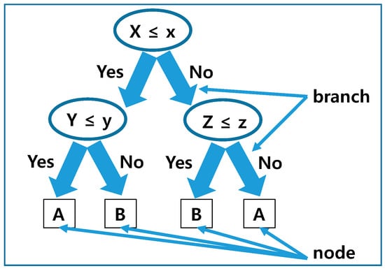
Figure 2.
Schematic diagram of classification. Independent variables are X, Y, and Z, and dependent variables are classified as A and B.
The classification criteria in CART maximize similarity and dissimilarity among groups based on the Gini index [15]. Because the branch divides repeatedly based on this method, a tree-shaped structure is hierarchically constructed. the visual expression is helpful in understanding and interpreting the results. The model has been widely used in many areas, including environmental sciences and epidemiological studies linking air pollution and human health [20,21,22,23,24,25,26].
The dependent variable in the model was categorized as days with relatively high (H) and low (L) numbers of daily deaths compared with the median number of daily deaths from respiratory disease. The median number of daily deaths during the analysis period was seven deaths. Thus, “H” indicates days where the number of deaths from respiratory disease is higher than seven, and “L” indicates days where the number of deaths is equal to or lower than seven.
Independent variables included the 1-h maximum pollutant concentrations (SO2, CO, O3, PM10, PM2.5, and NO2) and the 24-h average temperature. Air pollutant concentrations one to three days before the deaths were included in the independent variables to observe the influence from pollution prior to death. Temperature is known to have a relatively long-term effect compared with air pollution [10]. Therefore, temperatures from four to 20 days before the deaths were also included in the independent variables. To decrease the number of independent variables, average temperatures from four to 10 days and from 11 to 20 days were used instead of using temperatures on each day. A CART model’s accuracy does not increase even though the number of independent variables is increased if there is correlation between the independent variables [15]. The 1-h air pollutant concentration n days before the deaths is abbreviated as “Pollutant name”_max(n d) hereafter. For example, “O3_max(1 d)” indicates the 1-h maximum O3 concentration, one day before death. The average temperatures from 4 to 10 days and from 11 to 20 days are represented as “T(4–10 d)” and “T(11–20 d)”, respectively.
Taking into account the annual changes in air pollutant concentrations, an analysis was conducted for each month. For example, O3 concentration was especially high in May and June, and prolonged exposures to high ozone concentrations could be a direct cause of respiratory and eye diseases. On the other hand, particle concentrations were relatively high in winter. As such, it was difficult to accurately identify the factors causing mortality without adding seasonal distinctions into the analysis. Previous studies that used decision tree models to conduct studies related to air pollution also limited the analyses periods to several weeks and separate analyses were conducted for each season. For example, Chu et al. (2012) limited the analysis period to spring (from 28 April to 13 May 2009) to find factors that influenced ozone concentrations [24]. Park (2018) constructed independent models for each season to assess factors linked with cardiovascular disease [27].
3. Status of Air Pollution, Temperature, and the Number of Deaths Caused by Air Pollutants
3.1. Air Pollution and Temperature
Basic statistics of hourly SO2, CO, O3, NO2, PM10, and PM2.5 concentrations in Seoul, Korea, from 2008 and 2017 are illustrated as box plots in Appendix A (Figure A1). The plots show that SO2 and CO met the air quality standard at all times. Unsurprisingly, O3 exceeded the air quality standard from April to September; because strong sunlight accelerates O3 generation; as such, O3 generally increases in spring and summer [28,29,30]. The 24-h average NO2 exceeded the air quality standard from January to May and from October to December. Moreover, the 1-h average NO2 exceeded the standard regardless of the season. Much like NO2, the 24-h PM10 also exceeded the standard during the relatively cold seasons. One of the important causes of the higher PM10 concentrations during the cold seasons was the relatively low atmospheric mixing height because of a low ground temperature [31]. The year-round exceedance of PM2.5 shows how imperative it is to reduce PM2.5. Daily average temperatures showed clear seasonal changes; the highest temperature was 33.7 °C in August and the lowest value was −14.8 °C in January.
3.2. Number of Deaths Caused by Respiratory Disease
The number of deaths in Korea from 2008 to 2017 was around 2.6 million, so the annual average number of deaths was approximately 260,000. Differences in the number of deaths varied up to 15%, depending on the months. The mortality rate was relatively high in summer and winter, and relatively low in the spring and fall. Causes of death were cancers (28%), cardiovascular disease (22%), traffic accidents and suicides (11%), diabetes and liver disease (9%), respiratory disease (28%), and others (22%). DeLeon and Thruston (2003) found that the influence of air pollution on deaths was clear for the elderly, but less clear for others [32]. Accordingly, this study also focuses on persons aged 65 or older at time of death from respiratory disease (Table 1).
4. Results and Discussion
4.1. Linkage of Air Pollution and Temperature with Mortality from Respiratory Disease
Monthly average pollutant concentrations on days with a higher probability of deaths from respiratory disease were compared with those with lower probability of deaths to find the linkage between air pollution and deaths (Figure 3, Figure 4, Figure 5, Figure 6 and Figure 7). Differences in O3 concentrations were relatively large from May to August when high O3 concentrations were observed (Figure 3). Studies have shown that the adverse health effects from O3 are often found in industrialized cities, in which the production of O3 is accelerated by NOx and VOCs emissions [4,5,6,7]. Because strong sunlight is crucial for O3 production, high O3 levels are often found in spring, as was true in this case (Figure 3).
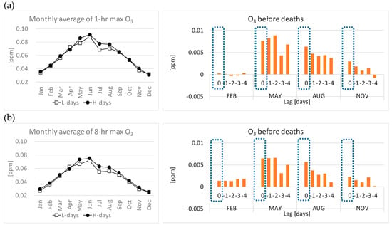
Figure 3.
Ozone (O3) concentrations on days with a higher or lower probability of deaths from respiratory disease, and those from zero to 5 days before death in February, May, August, and November between 2008 and 2017: (a) 1-h and (b) 8-h maximum O3 concentrations.
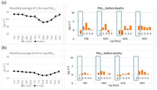
Figure 4.
Concentrations of particles less than 2.5 μm in size (PM2.5) on days with a higher or lower probability of deaths from respiratory disease, and those from zero to 5 days before deaths in February, May, August, and November between 2008 and 2017: (a) 1-h maximum and (b) 24-h average PM2.5 concentrations.
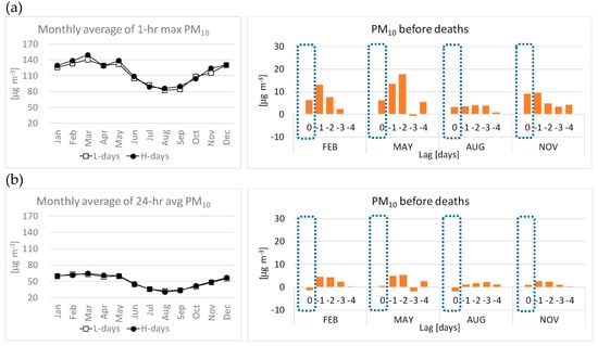
Figure 5.
PM10 concentrations on days with a higher or lower probability of deaths from respiratory disease, and those from zero to 5 days before deaths in February, May, August, and November between 2008 and 2017: (a) 1-h maximum and (b) 24-h average PM10 concentrations.
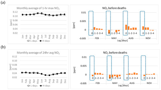
Figure 6.
Nitrogen dioxide (NO2) concentrations on days with a higher or lower probability of death from respiratory disease and those from zero to 5 days before deaths in February, May, August, and November between 2008 and 2017: (a) 1-h maximum and (b) 24-h average NO2 concentrations.

Figure 7.
Temperatures on days with a higher or lower probability of deaths from respiratory disease, and temperatures from zero to 5 days before deaths in May between 2008 and 2017.
The health impact of air pollution may appear within a few hours after exposure to pollution or several days afterward [5]. Consequently, a time delay may exist between the occurrence of high air pollution and death. To take this possibility into account, O3 concentrations up to five days before the day of death were analyzed; data in February, May, August, and November are presented as an example (Figure 3).
The O3 concentrations up to five days before recorded deaths were obviously higher than on days with lower numbers in May (Figure 3). The 1-h maximum O3 values in May on the days with high and low numbers of deaths were 86 ppb and 78.3 ppb, respectively, with a difference of 7.7 ppb (Figure 3a). Differences at 1, 2, 3, 4, and 5 days before death were 8.2 ppb, 8.9 ppb, 4.3 ppb, 6.8 ppb, and 5.6 ppb, respectively, indicating that the difference at 1–2 days before death was greater than that on the day of death. The 8-h average O3 values in May on days with high and low numbers of deaths were 72.9 ppb and 66.4 ppb, respectively, with a difference of 6.4 ppb (Figure 3b). Differences at 1, 2, 3, 4, and 5 days before death were 6.5 ppb, 6.6 ppb, 3.1 ppb, 5.0 ppb, and 4.1 ppb, respectively. The results indicated that O3 concentrations 1–2 days before death had a direct association with death, whereas O3 concentration 3–5 days before death had relatively less impact.
PM2.5 concentrations did not show clear differences between the days with high and low numbers of deaths (Figure 4). Differences in PM2.5 concentrations in August did not consistently increase or decrease on days before death. However, differences 1 day and 2 days before death increased in February, May, and November, while differences decreased 3, 4, and 5 days before death. These results imply that high PM2.5 1 day or 2 days before death is associated with deaths from respiratory disease, which is consistent with an existing study showing that deaths from cardiovascular disease occur a few days after high PM2.5 concentrations [33].
PM10 concentrations were relatively higher in winter and in spring (Figure 5). The high PM10 concentrations during relatively cold seasons are also related to the relatively low mixing height during the cold season, because pollutants can accumulate in the lower troposphere if the mixing height is low [34]. The period in which maximum PM10 concentrations were observed was consistent with days with an inflow of yellow dust from the west of Korea [35]. Differences in PM10 concentrations 1 day and 2 days before death were obvious in February, May, and November, which implied that PM10 concentrations one or two days before death had a large impact.
Monthly average NO2 concentrations on days with high numbers of deaths did not show a big difference to those with low numbers of deaths (Figure 6). NO2 concentrations from one to five days before days with high numbers of deaths differed little from those with low numbers of deaths. Such results do not necessarily mean that NO2 concentration was not a direct cause of death from respiratory disease, because the recorded monthly average concentration alone is insufficient for a thorough analysis of its effects. Accordingly, a decision tree model was introduced to permit closer observations of the health impacts of air pollution.
The average temperature on days from February to April with high numbers of deaths was lower than on days with a low number of deaths (Figure 7). This result is consistent with a previous study showing that high numbers of deaths by respiratory disease occurred on days with low temperatures in winter [36,37]. However, average temperatures on the days with high numbers of deaths were slightly higher in most cases than on the days with low numbers of deaths. This was partly because of the relatively low particle concentrations observed on cold days.
Air pollutant concentrations, especially those of secondary pollutants such as O3, are affected by meteorological conditions [29]. Moreover, when cold air masses move in from the relatively clean air of the northern polar area, particle concentrations tend to be low. Similar phenomena are observed in Vietnam as well. Hien et al. (2011) observed a reduced PM10 concentration from October to February in Hanoi, Vietnam, immediately before a cold surge occurred [38]. Similarly, temperature and air pollution are related. As a result, it is necessary to simultaneously analyze the effect of both air pollution and temperature on health to isolate the factors exacerbating respiratory disease.
4.2. Factors that Impact the Number of Deaths Caused by Respiratory Disease
4.2.1. Influence of 1-h Maximum Pollutant Concentrations on the Number of Deaths from Respiratory Disease
The decision tree model was used to observe the effect of pollutant concentrations on the number of deaths caused by respiratory disease. Originally, the model was constructed using all data, and the accuracy of the model was checked by the 10-fold cross validation error. Results showed that the error rate was 45%, indicating that the model did not accurately classify factors affecting high and low probability of death from respiratory disease, partly due to seasonal variations of pollutant concentrations. Thus, the analyses were conducted separately for each month.
The impact of air pollution and temperature on respiratory disease as analyzed with a CART model could be interpreted as follows (Figure 8). Here, “T(11–20 d)” became the basis for the first branch in January. This signified that the most important factor that impacted the risk of death was “T(11–20 d)”. Results showed that the risk of death was relatively low when “T(11–20 d)” was higher than 2.4 °C. When “T(11–20 d)” was 2.4 °C or lower, “PM2.5_max(1 d)”, the basis of the next branch, was checked to determine the risk of death. When “T(11–20 d)” was less than 2.4 °C and “PM2.5_max(1 d)” was higher than 95.5 μg∙m−3, the risk of death was relatively high. If the “PM2.5_max(1 d)” was 95.5 μg∙m−3 or less, “PM10_max(1 d)” was checked. If “PM10_max(1 d)” exceeded 125.5 μg∙m−3, the risk of death was relatively high. Assuming that “PM10_max(1 d)” was 125.5 μg∙m−3 or less, if the risk of death was relatively high when ”NO2_max(1 d)” was higher than 83 ppb, the risk of death was relatively low if “NO2_max(1 d)” was 83 ppb or less. Based on this, it was possible to analyze the linkage between temperature, PM10, PM2.5, and NO2 concentrations with the risk of death.
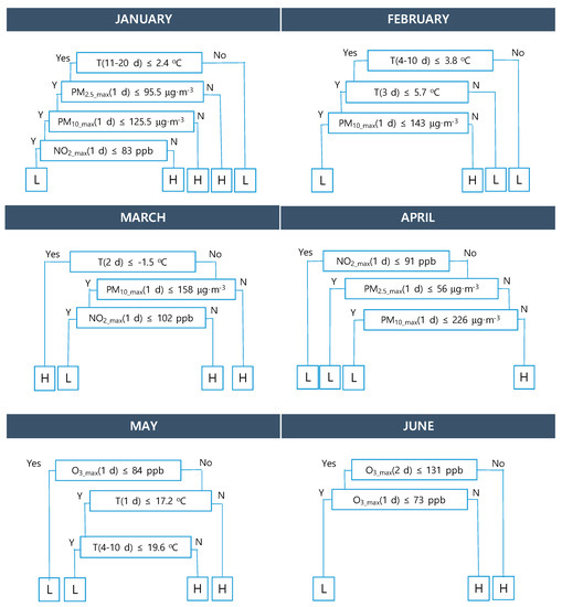
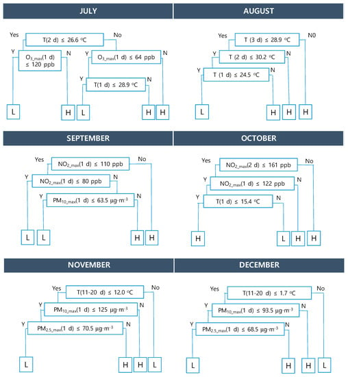
Figure 8.
Hourly maximum pollutant concentrations and temperature affecting the high (H) and low (L) probability of death from respiratory disease.
Here, “T(4–10 d)” was the most important factor in February. When “T(4–10 d)” exceeded 3.8 °C, the risk of death was relatively low. On the other hand, when “T(4–10 d)” was 3.8 °C or less, “T(3 d)” was checked to ascertain the risk of death. Even if “T(4–10 d)” was less than 3.8 °C, the risk of death was relatively low when “T(3 d)” was higher than 5.7 °C. However, when “T(4–10 d)” was less than 3.8 °C and “T(3 d)” was less than 5.7 °C, the risk of death differed depending on “PM10_max(1 d)”. Although the risk of death also increased when “PM10_max(1 d)” was higher than 143 μg∙m−3, it was relatively low when “PM10_max(1 d)” was 143 μg∙m−3 or below. Such results showed that “T(4–10 d)” was the most direct factor and that it was also important in February.
High PM10 concentrations were frequently observed, partly because of yellow dust in March (Figure A1e) [39,40]. “T(2 d)”, “PM10_max(1 d)”, and “NO2_max(1 d)” were among the important factors in March. “NO2_max(1 d)”, “PM2.5_max(1 d)”, and “PM10_max(1 d)" were related to the risk of death. Those results were consistent with previous studies that showed NO2 and particulate matter were directly related to deaths from respiratory disease. Dong et al. (2012) confirmed through a study in Shenyang, China, that the risk of death from respiratory disease increased when PM10 and NO2 concentrations were relatively high [41].
The 1-h maximum O3 concentrations before the deaths under study were the most important factors in May and in June. Burnet et al. (1997) illustrated the association between O3 concentrations one day before hospitalization and the number of hospitalized patients by analyzing patients in 16 cities in Canada from April 1981 to December 1991 [42]. Although “T(2 d)” was the most important factor in July, “O3_max(1 d)” was also closely related with the deaths. Reid et al. (2012) found that the risk of death increased when both O3 concentrations and temperatures were high [6].
The temperatures 1, 2, and 3 days before the deaths were linked with the cause of death in August (Figure 8). This result was consistent with a previous study that showed that the risk of death increased with higher temperatures in August [43]. “NO2_max(1 d)” was the most important factor relating to risk of death in September and in October. High PM10 and PM2.5 concentrations were frequently observed in November and in December, and “T(11–20 d)”, “PM10_max(1 d)”, and “PM2.5_max(1 d)” were important factors that determined the risk of death from respiratory disease.
The accuracy of results was ascertained through 10-fold cross validation of errors [44,45] (Table 2). Error rates were 27.6–42%, with the highest value in August. Errors were also relatively higher than for a similar study that analyzed factors influencing the number of deaths caused by cardiovascular disease [27]. The risk of death from respiratory disease was determined by only the temperature before deaths in August because pollutant levels were relatively low (Figure A1). One of the causes of the low pollutant concentrations in summer was the dilution of air pollution by the elevated mixing height [31]. In addition, the relatively high precipitation in summer inhibited the photochemical formation of O3 and accelerated the wet deposition of particles [46,47]. Accordingly, the risk of death was determined by only temperature in August, so the accuracy of the decision tree model may have been reduced.

Table 2.
Ten-fold cross validation errors from using a decision tree model to predict higher or lower probability of death from respiratory disease.
4.2.2. Influence of 24-h Average Pollutant Concentrations on the Number of Deaths from Respiratory Disease
The health impact of air pollution varied depending on how long people were exposed [13,14]. Zanobett et al. (2003) analyzed the influence of PM10 up to 40 days after exposure [48]. Results showed that when PM10 concentrations increased by 10 μg∙m−3, the risk of death from respiratory disease increased by 0.74%. The risk of death increased by five times if the exposure to air pollution lasted for more than a month. Therefore, to compare the effect of different exposure times, we analyzed the influence of 24-h average pollutant concentrations on deaths. Thus, the impact of the 24-h average pollutant levels was compared with that of the 1-h maximum pollutant concentrations analyzed in the previous section (Figure 9). The 24-h pollutant concentration n days before death is abbreviated as “Pollutant name”_avg(N d) hereafter. For example, “O3_avg(1 d)” indicates the 24-h average O3 concentration one day before death.
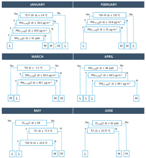
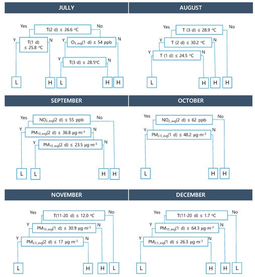
Figure 9.
Daily average pollutant concentrations and temperatures affecting the high (H) and low (L) probability of deaths from respiratory disease.
The first branch that classified the high and low risk of death in January was “T(11–20 d)”. The second branch was classified based on “PM10_avg(2 d)”. The risk of death was relatively low when “T(11–20 d)” was 2.4 °C or lower. When “T(11–20 d)” was higher than 2.4 °C, the risk of death was high if “PM10_avg(2 d)” was higher than 36.5 μg∙m−3. When “PM10_avg(2 d)” was less than 36.5 μg∙m−3, the risk of death was relatively high if “PM2.5_avg(2 d)” exceeded 29.4 μg∙m−3. When “PM2.5_avg(2 d)” was less than 29.4 μg∙m−3, the risk of death was relatively high if “NO2_avg(2d)” was higher than 52 ppb.
“T(4–10 d)” was directly related in February with the risk of death because of respiratory disease. When “T(4–10 d)” exceeded 3.8 °C, the risk of death was relatively low. When “T(4–10 d)” was less than 3.8 °C, the risk of death was relatively low only if “PM10_avg(2 d)” exceeded 52.8 μg∙m−3. When “PM10_avg(2 d)” was less than 52.8 μg∙m−3, the risk of death was classified as relatively high if “PM2.5_avg(2 d)” exceeded 25 μg∙m−3, but the risk was relatively low if “PM2.5_avg(2 d)” was lower than 25 μg∙m−3. Likewise, “T(4–10 d)”, “PM10_avg(2 d)”, and “PM2.5_avg(2 d)” were major factors in February.
“T(2 d)”, “PM10_avg(2 d)”, and “PM2.5_avg(2 d)” were factors in March that influenced the number of deaths from respiratory disease. Factors associated with the risk of death in April included “NO2_avg(2 d)”, ”PM10_avg(1 d)”, and “PM2.5_avg(1 d)”. High O3 concentrations were often observed in May. “O3_avg(1 d)” and temperatures before death were among the important factors. “O3_avg(2 d)” and “T(1 d)” were important in determining the risk of death.
Although “T(2d)” was the most important factor in July, “T(1 d)” and “O3_avg(1 d)” were also associated with deaths as well. The risk of death increased along with the higher temperatures in August. “NO2_avg(2 d)” was the most important factor related to the risk of death in September and in October. However, “T(11–20 d)” and “PM10_avg(1 d)” were the important risk factors in November and in December.
The 10-fold cross validation errors resulted in 24.1–42% of errors, depending on the month (Table 2). The errors were greater than those in a similar study that analyzed the relation between air pollution and cardiovascular disease [27]. We also conducted the analysis using a 3-day cumulative pollutant. Factors linked with the death from respiratory disease using a 3-day cumulative pollutant were similar to those using separate data on each day. However, the accuracy of the model using a 3-day cumulative pollutant was slightly worse than that using daily pollutant concentrations.
Errors analyzed using the 24-h average concentrations were slightly less than those analyzed using the 1-h maximum concentrations. The result indicated that the 24-h average concentrations were more directly related to the risk of death than 1-h maximum concentrations. Jerrett et al. (2004) confirmed differences in degrees of exposure leading to differences in mortality through research conducted in Hamilton, Canada [49]. If the subject of the analysis did not engage in outdoor activities during the period in which the 1-h maximum concentration was observed, a direct association between high pollutant concentrations and the risk of death did not occur, even though the 1-h maximum concentration was directly associated with health. Therefore, the results of this study alone should not be interpreted as proving that short-term exposure to extreme levels of pollution was relatively less hazardous to health than long-term exposure to elevated levels of air pollution.
5. Conclusions
The impact of air pollution on the risk of death from respiratory disease was analyzed. The analysis was conducted separately for each month to take into account the seasonal variability of air pollutant concentrations. The independent variables were 1-h maximum and 24-h average O3, PM2.5, PM10, NO2, SO2, and CO concentrations and temperatures. The dependent variables were classified into days with high (H) and low (L) numbers of deaths caused by respiratory disease. The results showed that a higher risk of mortality was observed on days from November to March, in which PM10/PM2.5 concentrations were relatively high and temperatures were low. NO2 was a crucial factor that influenced deaths from April to October. O3 was the most important factor in May and in June. The risk of death increased with the high temperatures in July and August.
The accuracy of results was validated through 10-fold cross validation errors. Although error rates using the 1-h maximum pollutant concentrations were 27.6–42%, those using the 24-h average pollutant concentrations slightly decreased to 24.9–42%. Thus, the 24-h average pollutant concentrations were found to be more directly related with mortality from respiratory disease.
The results obtained from this study may be used to establish policies to minimize the adverse health effects of air pollution. For example, when pollutant concentrations are forecast and are communicated to the public, daily average concentrations should be emphasized more than the hourly maximum concentrations. In addition, the results could be used to guide the public to refrain from outdoor activities when pollutant levels are elevated.
Conflicts of Interest
The author declares no conflict of interest.
Appendix A
Basic statistics of hourly SO2, CO, O3, NO2, PM10, and PM2.5 concentrations in Seoul, Korea, from 2008 and 2017 are illustrated as a box plot (Figure A1). The top and bottom of the box represented the 75th percentile (Q3) and 25th percentile (Q1), respectively. The tail’s upper most value expressed the smaller one between the maximum value and . On the other hand, the tail’s lower most value is the larger one between the minimum value and .
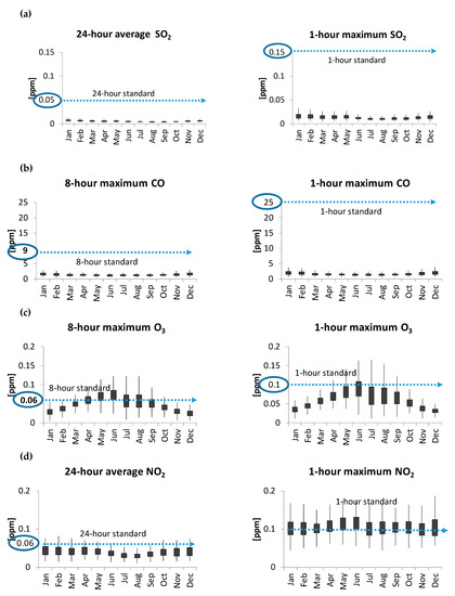
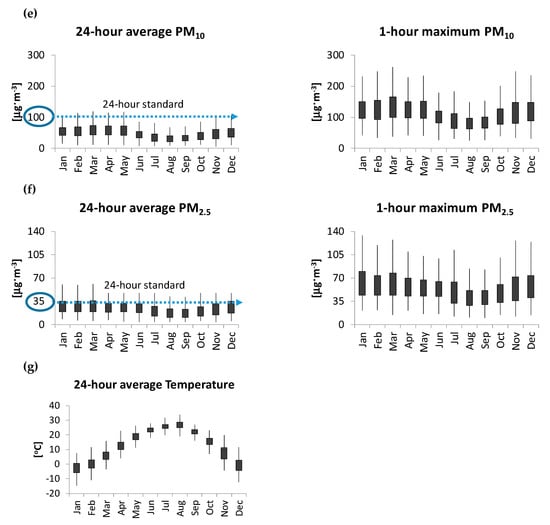
Figure A1.
Box plot of 1-h maximum, 8-h maximum, and 24-h average pollutant concentrations, and 24-h average temperatures between 2008 and 2017. (a) SO2, (b) CO, (c) O3, (d) NO2, (e) PM10 and (f) PM2.5, and (g) temperature.
References
- IPCC. Chapter 11. Human Health: Impacts, Adaptation, and Co-Benefits. In AR5 Climate Change 2014: Impacts, Adaptation, and Vulnerability; Working Group II contribution to the IPCC’s Fifth Assessment Repport; Intergovernmental Panel on Climage Change; Cambridge University Press: New York, NY, USA, 2014. [Google Scholar]
- Gao, F.; Calatayud, V.; García-Breijo, F.; Reig-Armiñana, J.; Feng, Z. Effects of elevated ozone on physiological, anatomical and ultrastructural characteristics of four common urban tree species in China. Ecol. Indic. 2016, 67, 367–379. [Google Scholar] [CrossRef]
- Wang, L.; He, X.; Chen, W. Effects of elevated ozone on photosynthetic CO2 exchange and chlorophyll a fluorescence in leaves of quercus mongolica grown in urban area. Bull. Environ. Contam. Toxicol. 2009, 82, 478–481. [Google Scholar] [CrossRef] [PubMed]
- Wu, Y.-L.; Lin, C.-H.; Lai, C.-H.; Lai, H.-C.; Young, C.-Y. Effects of Local Circulations, Turbulent Internal Boundary Layers, and Elevated Industrial Plumes on Coastal Ozone Pollution in the Downwind Kaohsiung Urban-Industrial Complex. Terr. Atmos. Ocean. Sci. 2010, 21, 343–357. [Google Scholar] [CrossRef]
- Bell, M.L.; McDermott, A.; Zeger, S.L.; Samet, J.M.; Dominici, F. Ozone and short-term mortality in 95 US urban communities, 1987–2000. JAMA 2004, 292, 2372–2378. [Google Scholar] [CrossRef]
- Reid, C.E.; Snowden, J.M.; Kontgis, C.; Tager, I.B. The Role of Ambient Ozone in Epidemiologic Studies of Heat-Related Mortality. Environ. Health Perspect. 2012, 120, 1627–1630. [Google Scholar] [CrossRef] [PubMed]
- Stafoggia, M.; Forastiere, F.; Faustini, A.; Biggeri, A.; Bisanti, L.; Cadum, E.; Cernigliaro, A.; Mallone, S.; Pandolfi, P.; Serinelli, M.; et al. Susceptibility factors to ozone-related mortality: A population-based case-crossover analysis. Am. J. Respir. Crit. Care Med. 2010, 182, 376–384. [Google Scholar] [CrossRef]
- Seven Million Premature Deaths Annually Linked to Air Pollution. Available online: https://www.who.int/mediacentre/news/releases/2014/air-pollution/en/ (accessed on 2 October 2019).
- Hong, Y.-C.; Lee, J.-T.; Kim, H.; Kwon, H.-J. Air pollution: A new risk factor in ischemic stroke mortality. Stroke 2002, 33, 2165–2169. [Google Scholar] [CrossRef]
- Jackson, J.E.; Yost, M.G.; Karr, C.; Fitzpatrick, C.; Lamb, B.K.; Chung, S.H.; Chen, J.; Avise, J.; Rosenblatt, R.A.; Fenske, R.A. Public health impacts of climate change in Washington State: Projected mortality risks due to heat events and air pollution. Clim. Chang. 2010, 102, 159–186. [Google Scholar] [CrossRef]
- Son, J.-Y.; Bell, M.L.; Lee, J.-T. Individual exposure to air pollution and lung function in Korea: Spatial analysis using multiple exposure approaches. Environ. Res. 2010, 110, 739–749. [Google Scholar] [CrossRef]
- Forns, J.; Dadvand, P.; Esnaola, M.; Alvarez-Pedrerol, M.; López-Vicente, M.; Garcia-Esteban, R.; Cirach, M.; Basagaña, X.; Guxens, M.; Sunyer, J. Longitudinal association between air pollution exposure at school and cognitive development in school children over a period of 3.5 years. Environ. Res. 2017, 159, 416–421. [Google Scholar] [CrossRef]
- Ljungman, P.L.; Li, W.; Rice, M.B.; Wilker, E.H.; Schwartz, J.; Gold, D.R.; Koutrakis, P.; Benjamin, E.J.; Vasan, R.S.; Mitchell, G.F.; et al. Long- and short-term air pollution exposure and measures of arterial stiffness in the Framingham Heart Study. Environ. Int. 2018, 121, 139–147. [Google Scholar] [CrossRef] [PubMed]
- Lee, H.; Myung, W.; Jeong, B.-H.; Choi, H.; Jhun, B.W.; Kim, H. Short- and long-term exposure to ambient air pollution and circulating biomarkers of inflammation in non-smokers: A hospital-based cohort study in South Korea. Environ. Int. 2018, 119, 264–273. [Google Scholar] [CrossRef] [PubMed]
- Breiman, L.; Friedman, J.; Stone, C.J.; Olshen, R.A. Classification and Regression Trees (Wadsworth Statistics/Probability), 1st ed.; Chapman and Hall/CRC: Boca Raton, FL, USA, 1984. [Google Scholar]
- Air Quality Data. Available online: https://www.airkorea.or.kr/eng (accessed on 2 October 2019).
- Synoptic Meteorological Data. Available online: https://data.kma.go.kr (accessed on 2 October 2019).
- Microdata Integrated Service. Available online: https://mdis.kostat.go.kr (accessed on 2 October 2019).
- Hastie, T.; Tibshirani, R.; Friedman, J. The Elements of Statistical Learning; Springer Science and Business Media LLC: New York, NY, USA, 2009. [Google Scholar]
- Venkatasubramaniam, A.; Wolfson, J.; Mitchell, N.; Barnes, T.; Jaka, M.; French, S. Decision trees in epidemiological research. Emerg. Themes Epidemiol. 2017, 14, 11. [Google Scholar] [CrossRef]
- Wolfson, J.; Venkatasubramaniam, A. Branching Out: Use of Decision Trees in Epidemiology. Curr. Epidemiol. Rep. 2018, 5, 221–229. [Google Scholar] [CrossRef]
- Bae, J.-M. Clinical Decision Analysis using Decision Tree. Epidemiol. Health 2014, 36, 201425. [Google Scholar] [CrossRef] [PubMed]
- Le Ray, I.; Lee, B.; Wikman, A.; Reilly, M. Evaluation of a decision tree for efficient antenatal red blood cell antibody screening. Epidemiology 2018, 29, 453–457. [Google Scholar] [CrossRef]
- Chu, H.-J.; Lin, C.-Y.; Liau, C.-J.; Kuo, Y.-M. Identifying controlling factors of ground-level ozone levels over southwestern Taiwan using a decision tree. Atmos. Environ. 2012, 60, 142–152. [Google Scholar] [CrossRef]
- Gardner, M.; Dorling, S. Statistical surface ozone models: An improved methodology to account for non-linear behaviour. Atmos. Environ. 2000, 34, 21–34. [Google Scholar] [CrossRef]
- Park, S.-K. Assessing Factors Linked with Ozone Exceedances in Seoul, Korea through a Decision Tree Algorithm. J. Environ. Sci. Int. 2016, 25, 191–216. [Google Scholar] [CrossRef]
- Baranski, L.; Jankowiak, L.; Rozemski, K. Seasonal changes of the spatial distribution of ozone content over Central Europe from TOVS/NOAA satellite data. Adv. Space Res. 1993, 13, 325–328. [Google Scholar] [CrossRef]
- Roy, S.; Beig, G.; Jacob, D. Seasonal distribution of ozone and its precursors over the tropical Indian region using regional chemistry-transport model. J. Geophys. Res. Space Phys. 2008, 113, 21307. [Google Scholar] [CrossRef]
- Scheel, H.E.; Areskoug, H.; Geiss, H.; Gomiscek, B.; Granby, K.; Haszpra, L.; Klasinc, L.; Kley, D.; Laurila, T.; Lindskog, A.; et al. On the Spatial Distribution and Seasonal Variation of Lower-Troposphere Ozone over Europe. J. Atmos. Chem. 1997, 28, 11–28. [Google Scholar] [CrossRef]
- Kim, S.-W.; Yoon, S.-C.; Won, J.-G.; Choi, S.-C. Ground-based remote sensing measurements of aerosol and ozone in an urban area: A case study of mixing height evolution and its effect on ground-level ozone concentrations. Atmos. Environ. 2007, 41, 7069–7081. [Google Scholar] [CrossRef]
- De Leon, S.F.; Thurston, G.D.; Ito, K. Contribution of Respiratory Disease to Nonrespiratory Mortality Associations with Air Pollution. Am. J. Respir. Crit. Care Med. 2003, 167, 1117–1123. [Google Scholar] [CrossRef] [PubMed]
- Dabass, A.; Talbott, E.O.; Venkat, A.; Rager, J.; Marsh, G.M.; Sharma, R.K.; Holguin, F. Association of exposure to particulate matter (PM2.5) air pollution and biomarkers of cardiovascular disease risk in adult NHANES participants (2001–2008). Int. J. Hyg. Environ. Health 2016, 219, 301–310. [Google Scholar] [CrossRef] [PubMed]
- Nath, S.; Patil, R.S. Prediction of air pollution concentration using an in situ real time mixing height model. Atmos. Environ. 2006, 40, 3816–3822. [Google Scholar] [CrossRef]
- Han, Y.-J.; Holsen, T.M.; Hopke, P.K.; Cheong, J.-P.; Kim, H.; Yi, S.-M. Identification of source locations for atmospheric dry deposition of heavy metals during yellow-sand events in Seoul, Korea in 1998 using hybrid receptor models. Atmos. Environ. 2004, 38, 5353–5361. [Google Scholar] [CrossRef]
- Gómez-Acebo, I.; Llorca, J.; Dierssen, T. Cold-related mortality due to cardiovascular diseases, respiratory diseases and cancer: A case-crossover study. Public Health 2012, 127, 252–258. [Google Scholar] [CrossRef]
- Kim, D.W.; Deo, R.C.; Chung, J.H.; Lee, J.S. Projection of heat wave mortality related to climate change in Korea. Nat. Hazards 2016, 80, 623–637. [Google Scholar] [CrossRef]
- Hien, P.; Loc, P.; Dao, N. Air pollution episodes associated with East Asian winter monsoons. Sci. Total. Environ. 2011, 409, 5063–5068. [Google Scholar] [CrossRef]
- Park, S.K. Assessing the impact of air pollution on mortality rate from cardiovascular disease in Seoul, Korea. Environ. Eng. Res. 2018, 23, 430–441. [Google Scholar] [CrossRef]
- Kim, K.; Macdonald, A.M.; Park, K.; Kim, H.-C.; Yoon, H.-I.; Yang, E.J.; Jung, J.; Kim, J.-H.; Lee, J.; Choi, T.; et al. Spatial and temporal variabilities of spring Asian dust events and their impacts on chlorophyll-a concentrations in the western North Pacific Ocean. Geophys. Res. Lett. 2017, 44, 1474–1482. [Google Scholar]
- Park, S.-U.; Choe, A.; Park, M.-S. A simulation of Asian dust events observed from 20 to 29 December 2009 in Korea by using ADAM2. Asia-Pacific J. Atmos. Sci. 2013, 49, 95–109. [Google Scholar] [CrossRef]
- Dong, G.-H.; Zhang, P.; Sun, B.; Zhang, L.; Chen, X.; Ma, N.; Yu, F.; Guo, H.; Huang, H.; Lee, Y.L.; et al. Long-Term Exposure to Ambient Air Pollution and Respiratory Disease Mortality in Shenyang, China: A 12-Year Population-Based Retrospective Cohort Study. Respiration 2012, 84, 360–368. [Google Scholar] [CrossRef]
- Brook, J.R.; Yung, W.T.; Dales, R.E.; Burnett, R.T.; Krewski, D. Association between Ozone and Hospitalization for Respiratory Diseases in 16 Canadian Cities. Environ. Res. 1997, 72, 24–31. [Google Scholar]
- Lee, W.; Choi, H.M.; Kim, D.; Honda, Y.; Guo, Y.L.; Kim, H. Temporal changes in morality attributed to heat extremes for 57 cities in Northeast Asia. Sci. Total Environ. 2018, 616, 703–709. [Google Scholar] [CrossRef]
- Camacho, J.; Ferrer, A.; Páez, J.C. Cross-validation in PCA models with the element-wise k-fold (ekf) algorithm: Practical aspects. Chemom. Intell. Lab. Syst. 2014, 131, 37–50. [Google Scholar] [CrossRef]
- Grimm, K.J.; Mazza, G.L.; Davoudzadeh, P. Model Selection in Finite Mixture Models: A k-Fold Cross-Validation Approach. Struct. Equ. Model. 2017, 24, 246–256. [Google Scholar] [CrossRef]
- Lim, C.; Jang, J.; Lee, I.; Kim, G.; Lee, S.M.; Kim, Y.; Kim, H.; Kaufman, A.J. Sulfur isotope and chemical compositions of the wet precipitation in two major urban areas, Seoul and Busan, Korea. J. Asian Earth Sci. 2014, 79, 415–425. [Google Scholar] [CrossRef]
- Wang, B.; Ding, Q.; Jhun, J.G. Trends in Seoul (1778–2004) summer precipitation. Geophys. Res. Lett. 2006, 33, L15803. [Google Scholar] [CrossRef]
- Zanobetti, A.; Schwartz, J.; Samoli, E.; Gryparis, A.; Touloumi, G.; Peacock, J.; Anderson, R.H.; Le Tertre, A.; Bobros, J.; Celko, M.; et al. The temporal pattern of respiratory and heart disease mortality in response to air pollution. Environ. Health Perspect. 2003, 111, 1188–1193. [Google Scholar] [CrossRef] [PubMed]
- Jerrett, M.; Burnett, R.T.; Brook, J.; Kanaroglou, P.; Giovis, C.; Finkelstein, N.; Hutchison, B. Do socioeconomic characteristics modify the short term association between air pollution and mortality? Evidence from a zonal time series in Hamilton, Canada. J. Epidemiol. Community Health 2004, 58, 31–40. [Google Scholar] [CrossRef] [PubMed]
© 2019 by the author. Licensee MDPI, Basel, Switzerland. This article is an open access article distributed under the terms and conditions of the Creative Commons Attribution (CC BY) license (http://creativecommons.org/licenses/by/4.0/).