1. Introduction
Clouds can act as a greenhouse ingredient to warm the Earth by trapping outgoing longwave radiation and can also cool the earth by reflecting shortwave solar radiation [
1]. The net effect of these two competing processes depends on the height, type, and optical properties of the clouds. Clouds also play a major role in the hydrological cycle, acting as the connection between atmospheric water vapor and rain [
2], and are involved in climate feedback processes [
3,
4]. Cloud microphysical properties are an important characteristic of clouds, as their ability to produce rain and snow, generate lightning, and contribute to the radiation balance of the earth depends on local air motions but also on their individual microphysical properties [
5]. The chemical composition of clouds is also an important issue. The chemical and biological transformations occurring in clouds perturb both the gas phase chemical composition and the microphysical and chemical properties of aerosols acting as cloud condensation nuclei (CCN). These transformations could, therefore, impact air quality and cloud formation. For example, a recent study showed that cloud microorganisms isolated at the puy de Dôme station (PUY) were able to produce biosurfactants [
6], which could favor the conversion of aerosol into cloud droplets, based on Köhler’s theory [
7].
In situ techniques for clouds’ microphysical and chemical characterizations are currently deployed at altitude sites that are privileged sites for studying clouds during specific measurement campaigns or continuous observations. The monitoring of cloud properties from the situ measurements at high-altitude sites over long term periods is one of the goals of the ACTRIS research infrastructure [
8], in order to assess multi-decanal tendencies in cloud properties over Europe. In pursuit of a harmonized European cloud in situ data set, an inter-comparison campaign, performed at PUY in May 2013, gathered a unique set of cloud instruments, which are operated simultaneously in ambient air conditions and in a wind tunnel, for assessing the inter-instrumental variability of microphysical cloud measurements. The study highlighted the good general agreement in the sizing abilities of the different instruments but also some discrepancies in their ability to assess the amplitude and variability of the cloud droplet number concentration [
9]. Long-term chemical and biological composition are also investigated [
10,
11,
12], with the objective to classify clouds based on their chemical properties and analyze their backward trajectories. Specific field campaigns are regularly organized, where clouds are sampled and analyzed [
13,
14].
Apart from the detailed cloud microphysical structure, which provides key information for evaluating the impact of clouds on climate, information on whether a cloud is present with good temporal resolution is already valuable for an atmospheric observation station. For example, this information can be useful for:
- -
The validation of cloud sensors aboard satellite missions;
- -
The organization of ongoing or future field measurement campaigns. The statistical analysis of cloud presence depending on the days and seasons is valuable information for choosing a suitable date for a field campaign focused on cloud studies or, on the contrary, to avoid the presence of clouds for field campaigns that require clear sky conditions;
- -
The constitution of sets of metadata to analyze other observations (gas, aerosol, etc.).
- -
Knowledge of cloud occurrence thus offers important auxiliary data for altitude observation sites, which must be established with reliable instruments and methods. Probes, such as the particulate volume monitor (PVM) Gerber, can provide this information, but there may be problems with the reliability or continuity of the data for a long-term survey due to icing conditions. More generally, not all sites are equipped with microphysical probes, which are expensive and need assistance under harsh meteorological conditions, such as intensive icing.
A low-cost alternative to cloud microphysical probes is presented here for the detection of clouds at and below a high-altitude site. The objectives of this article are to demonstrate the feasibility and reliability of the automatic detection of clouds from camera images on the PUY site, to present comparisons of this new product with other data, and to provide the first cloud climatology study for the site.
2. Instruments and Data
2.1. Network and All-Sky Cameras
Cézeaux and PUY are two instrumented sites of CO-PDD (Cézeaux-Aulnat-Opme-Puy de Dôme), a full instrumented platform for atmospheric research, which is nationally labeled by CNRS, the French national center for scientific research, and has been recognized as a global GAW (global atmospheric watch, station PUY) station since 2014 [
15].
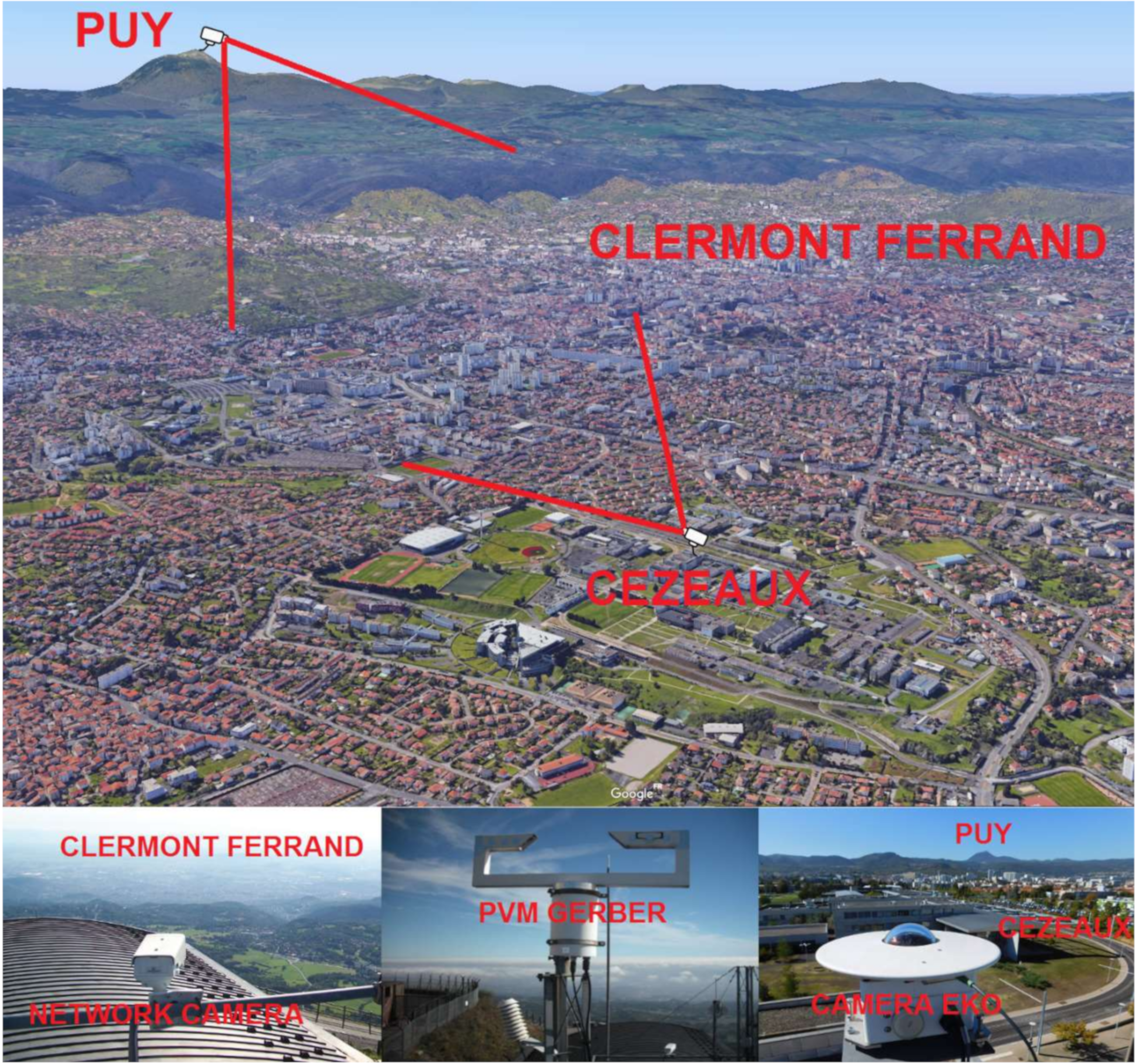
Two network cameras are in operation—one at the Cézeaux site looking towards PUY, and the other at PUY looking towards the Clermont-Ferrand area. Cézeaux is a campus at the University Clermont Auvergne, located south of the Clermont-Ferrand city, at an altitude of 410 m a.s.l. PUY is the mountain station, located 12 km east of Cézeaux, at an altitude 1465 m a.s.l. (
Figure 1).
The two network cameras are Axis P1343 cameras, which are widely used in daytime and nighttime video surveillance. These cameras capture 600 × 800 pixel images every ten minutes in an uncompressed JPEG format. More technical details on the cameras are available on the Axis manufacturer’s website [
16].
The images taken by the Cézeaux and PUY cameras are available in real time on the website of the Observatoire de Physique du Globe de Clermont-Ferrand [
17]. The percentage of available network camera images related to the maximum number of images theoretically available varied from 72% to 100%, except for May 2018 (55%,
Table 1). Images were missed due to problems while writing the images, data transmission, electrical shutdown of the station, or accumulation of snow in front of the camera during winter.
In addition, an all-sky camera has been in operation at Cézeaux since December 2015. The all-sky camera is an EKO SRF-02, a fully automatic imaging system that captures 1024 × 768 pixel JPEG images of the total sky at different exposures every 2 min. When the sky images are captured, a real time cloud fraction (CF) is automatically calculated by the acquisition software, which offers great flexibility and functions. For example, the software is able to define the area of interest by horizon masking. A more optimized CF evaluation was also performed by the software ELIFAN [
18], which is used in this study.
The SRF-02 is connected to a computer network through a standard Ethernet interface. The all-sky camera is equipped with an air pump and drying cartridge. In this paper, the methodology is based on camera images from the PUY camera, and PVM Gerber has been used for validation. In this work, 524 days of operation of the all-sky cameras have been used from December 2015 to December 2018.
2.2. PVM Gerber
Gerber PVM-100 is a ground-direct scattering laser spectrophotometer for cloud droplet volume measurements and is manufactured by Gerber Scientific, Inc., Reston, Virginia (USA). It measures the cloud liquid water content (LWC), the surface of the droplets, and determines the effective radius of the droplets [
19,
20].
A laser light emitted at a wavelength of λ = 0.780 μm is dispersed by the cloud droplets passing through the sampling volume of the 3 cm−3 probe. This light is collected by a lens system whose angle varies from 0.25° to 5.2°. The scattered light is converted into a signal that is proportional to the droplet density (or LWC) and the particle surface density (PSA) (Gerber et al., 1994). This light measures the cloud water content (in the range of 0.002–10 g m−3), the total particle area, and, deduced from these values, the effective droplet radius (in the range of 2–70 μm).
In this paper, we use the LWC measured with the PVM cloud probe as a reference to establish the presence of clouds at the station. If the LWC > 0 g m−3, we consider the station to be under cloudy conditions. Otherwise, if LWC = 0 g m−3, the summit is considered to be not cloudy.
2.3. CATS (Cloud-Aerosol Transport System)
The NASA cloud-aerosol transport system (CATS) is a lidar onboard the International Space Station (ISS) that provides vertical profiles of atmospheric aerosols and clouds [
21]. CATS was in operation from February 2015 to October 2017.
The CF parameter is deduced from the calibrated vertical profiles of the backscattered signals at 1064 nm [
22], with an algorithm separating low level clouds and aerosols similar to the cloud-aerosol lidar and infrared pathfinder satellite observation (CALIPSO) algorithm [
23]. More details on the CATS inversion algorithms and data can be found in the CATS data product catalog [
24].
In the present work, we have used cloud detections from the CATS level 2 operation cloud layer product (L2O-CLay). This product includes cloud layers detected horizontally and averaging between 1 to 60 km, reported every 5 km along-track. To document the daily variability of the cloud detections in the present study, we extracted all profiles measured by CATS in a 5° × 5° latitude-longitude box centered on PUY, with a feature type score above 5 (as in [
23]), and indexed them according to the local time when the observation was made.
2.4. Meteosat/SEVIRI
The SEVIRI (spinning enhanced visible and infrared imager) onboard MSG (METEOSAT second generation) geostationary satellite is a visible and infrared multi-channel imager that operates on a 15 min repeat cycle. The spatial resolution at a sub-satellite point is 3 × 3 km2 and about 3.2 × 5.3 km2 close to PUY. The presence of clouds can be detected for each elementary pixel, and the cloud occurrence can thus be established.
Cloud detection is also divided into types in the vertical dimension. The cloud type classification used here is obtained from the satellite application facility for NoWCasting (SAF NWC) algorithm [
25], developed by Derrien and Le Gleau [
26,
27]. In the SAF NWC algorithm, cloud detection and classification rely on multi-spectral threshold tests applied at the pixel scale to a set of spectral and textural features. Thresholds are values that depend on illumination and viewing geometry, as well as geographical location. These values are computed using ancillary data and radiative transfer models.
After sorting between cloud free and cloud contaminated pixels, cloudy pixels are classified into ten sets, according to the altitude of the cloud cover summit. For high-topped clouds, a sub-division is performed according to their semi-transparency.
In this study, we consolidate these ten classes into five main classes: low-topped clouds, mid-topped clouds, opaque high-topped clouds, non-opaque high-topped clouds, and partial cloud cover. For pixels belonging to the “partial cloud class”, no pressure information is available. Clouds partly covering these pixels can be at any level. Recently, this cloud type classification has been evaluated using CALIOP lidar data [
28]. High-topped clouds, including thin cirrus clouds, are well observed. Low-topped clouds over land are less well observed when they are thin or only partially cover the pixels or during nigh-time when they are close to the ground.
2.5. ECMWF Reanalysis
ERA-5 is a recent global atmospheric reanalysis tool produced by ECMWF, which has available since 2018 and succeeded ERA-Interim. ERA-5 contains several improvements to ERA-Interim: the use of more recent versions of data assimilation methods and parameterizations of Earth processes, as well as improved temporal and spatial resolutions from 6 h in ERA-Interim to hourly in ERA-5, and from 79 km in the horizontal dimension and 60 levels in the vertical in ERA-Interim to 31 km and 137 levels in ERA-5 [
29].
In this work, we extract the parameter “fraction of cloud cover” from the ECMWF ERA-5 archive at the 850 pressure level from 1 January 2013 to 31 December 2018 at an hourly temporal resolution and a 0.125° spatial resolution and linearly interpolate at the exact location of PUY (45.77° N, 2.95° E). This parameter is the proportion of a grid box covered by cloud (liquid or ice) and varies between zero and one.
Notably, this parameter is comparable to the CF established with the all-sky camera, but it is different from the cloud occurrence established based on the temporal evolution of the cloud or no cloud binary parameter with the network camera or Meteosat SEVIRI. In this work, we will thus use the term cloud fraction (CF in abbreviated form) when the cloud cover is established spatially and “cloud occurrence frequency” (COF in abbreviated form) when it is established temporally.
3. Methodology of Network Camera Image Processing
The camera produces images in the joint photographic experts group (JPEG) format. A JPEG image is a matrix of pixels ranging from the value 0 (for low light) to 255 (for high brightness) in 3 channels for red green and blue colors. It is possible to access and manipulate the digital accounts of the images’ pixels with scientific software. We used the commercial MATLAB software environment [
30], but the code can easily be adapted for open access software, such as Python [
31].
The methodology is based on the detection of contrast in specific areas of the image. The detection of contrast is based on the standard deviation of the pixel values on an area of the image. When the camera is in a cloud, the image has little contrast, and the standard deviation value is low. On the contrary, for a non-cloudy situation, an area centered on Clermont-Ferrand will have high contrast corresponding to a high value of standard deviation.
This camera works similarly with any of the three colors; in this work we chose red. This method works during the day, but also at night thanks to night lighting in the city.
A second zone centered on the horizon of the Livradois-Forez Mountains makes it possible to distinguish individual clouds in situations where a sea of clouds is present: low clouds have an altitude of the top of the cloud layer less than the altitude of PUY (1465 m). The sizes of the zones are 100 × 350 pixels (Clermont-Ferrand) and 50 × 270 pixels (Livradois-Forez).
The camera may move slightly because of strong wind or maintenance. It is then necessary to calculate the location of the zones relative to a mark on the image to correct possible movements of the camera. We also had to remove incorrect images with rain drops or snow on the lens of the camera.
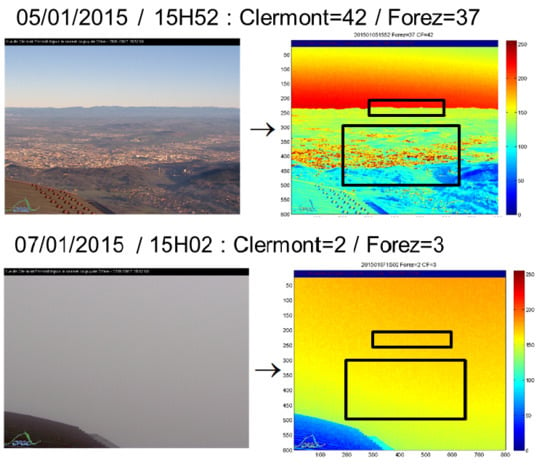
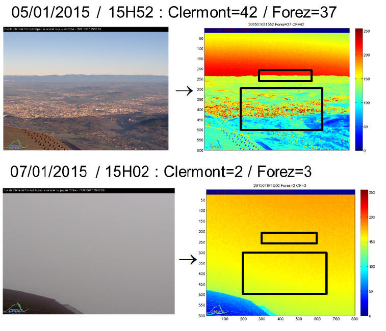
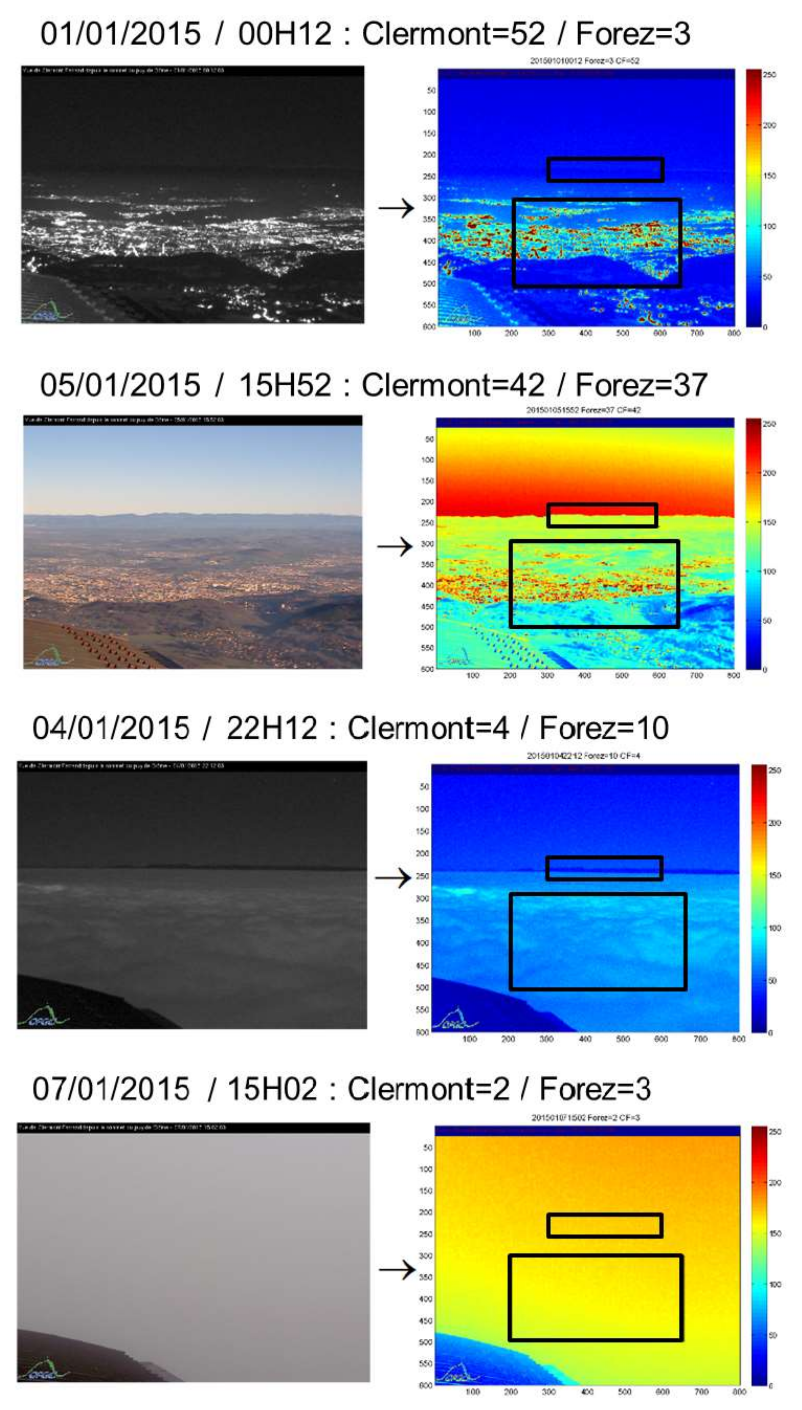
Figure 2 shows some examples of these images and MATLAB processing in cloudy, sea of clouds, and clear sky conditions. Finally, it is necessary to define a threshold value for the standard deviation, which separates cloudy and clear sky situations.
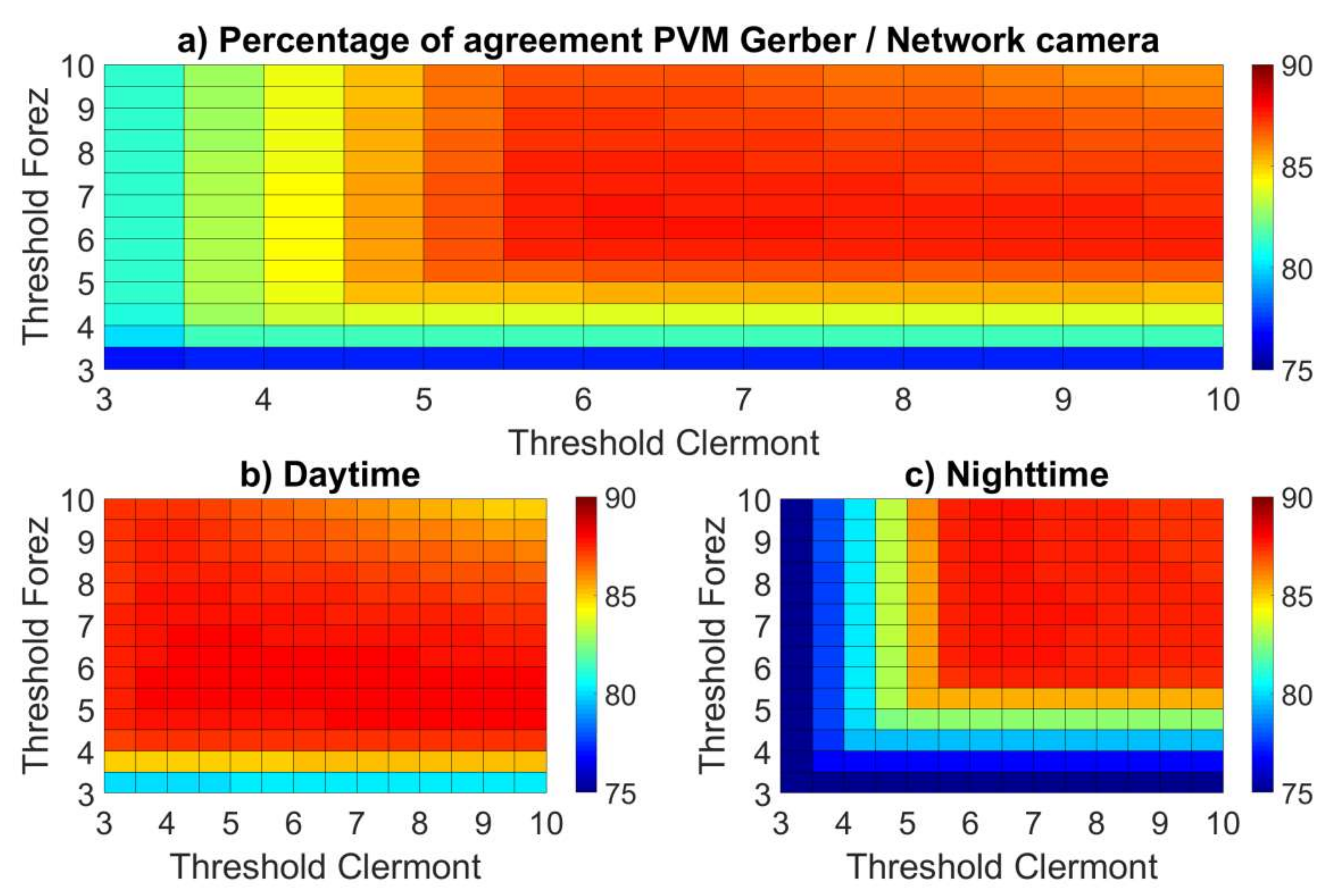
Figure 3 presents a sensitivity analysis applied to the total set of images (2013–2018). The maximum agreement is obtained with a threshold value of 6 for the two zones (Clermont and Livradois-Forez). Agreement is obtained by dividing the number of cases where the two systems (camera and PVM) obtain the same result (cloudy or clear sky) by the total number of coincidences (the time difference between the image taking and the PVM measurement is less than 2 min). The detection of clouds depends on the signal to noise ratio of the camera, which may be different during the day and night. In order to check the robustness of the method during day and night, we have also applied a sensitivity analysis only for daytime (
Figure 3b) and nighttime (
Figure 3c) images. The results show that a threshold value of 6 correctly separates cloudy and clear sky situations, as well as day and night (between 85% and 90% agreement). Since the threshold value of 6 separates a cloudy situation from a non-cloudy situation, we consider that below 5.5 the image will be considered cloudy, above 6.5 it will be considered cloudless, and between these two values it will be considered indeterminate.
4. Validation
The COF monthly average was calculated over the period 2013–2018 by dividing the number of images in which a cloud is detected, following the method described in
Section 3, by the total number of recorded images. For validation purposes, this parameter is compared to the COF deduced from the PVM Gerber measurements. The results are shown in
Figure 4.
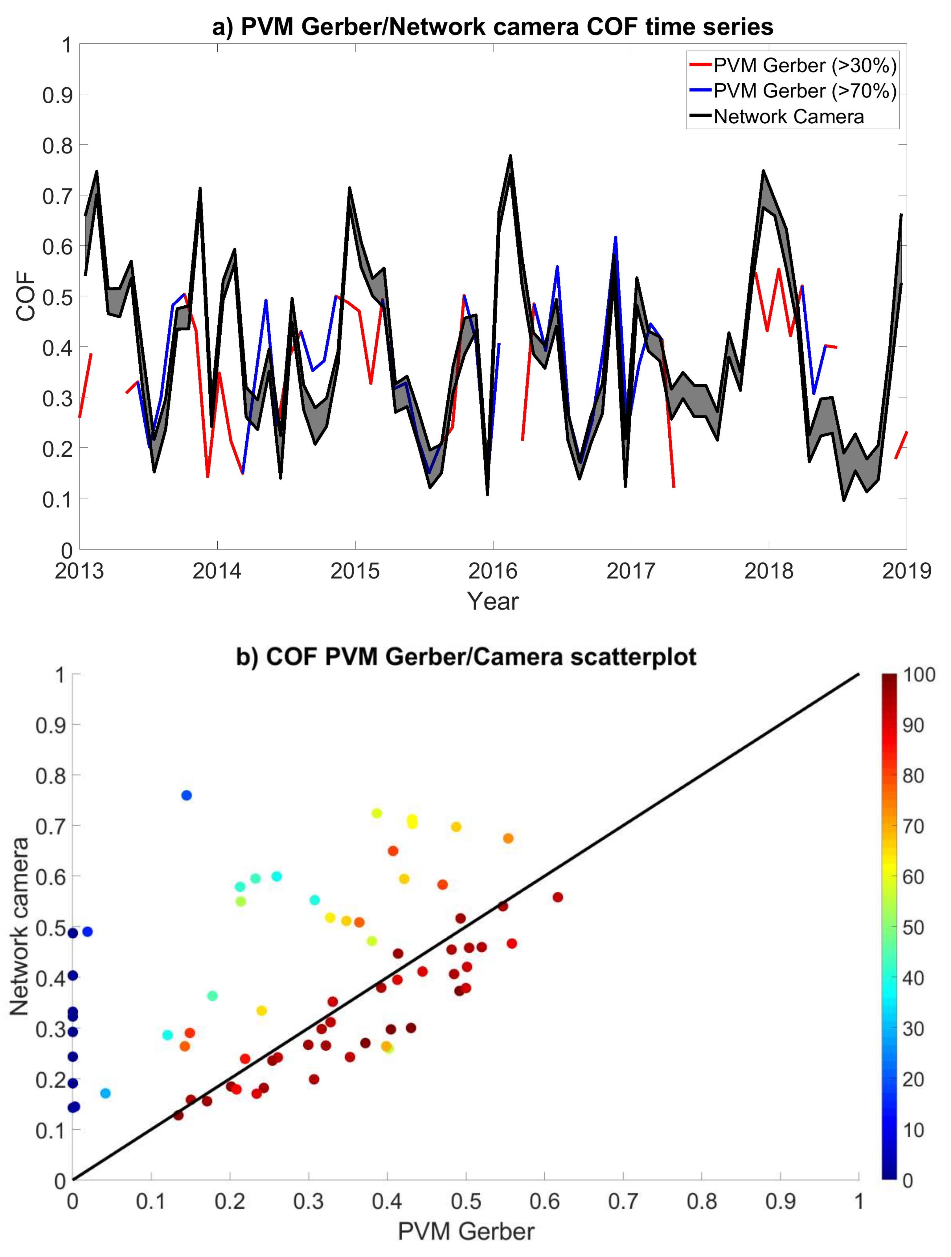
Figure 4a shows a very good agreement between the two techniques over some periods.
Figure 4b shows that the months during which a large difference is found between the two technics correspond to a very low operating rate of the PVM Gerber by taking all the measurements available, not only the measurements coincident with the camera.
Table 2 provides the correlation coefficients between the two series with different operating thresholds of the Gerber. The more the Gerber works continuously, the higher the correlation between the two series. The correlation coefficient reaches 0.83 when the PVM Gerber is working more than 70% of the time.
5. Diurnal, Seasonal, and Inter-Annual Variations of the COF at PUY
The camera data processing methodology for the estimation of the COF presented in
Section 3 and validated in
Section 4 was applied to all the PUY images from 2013 to 2018 to analyze the temporal variations at different time scales: diurnal, seasonal, and inter-annual.
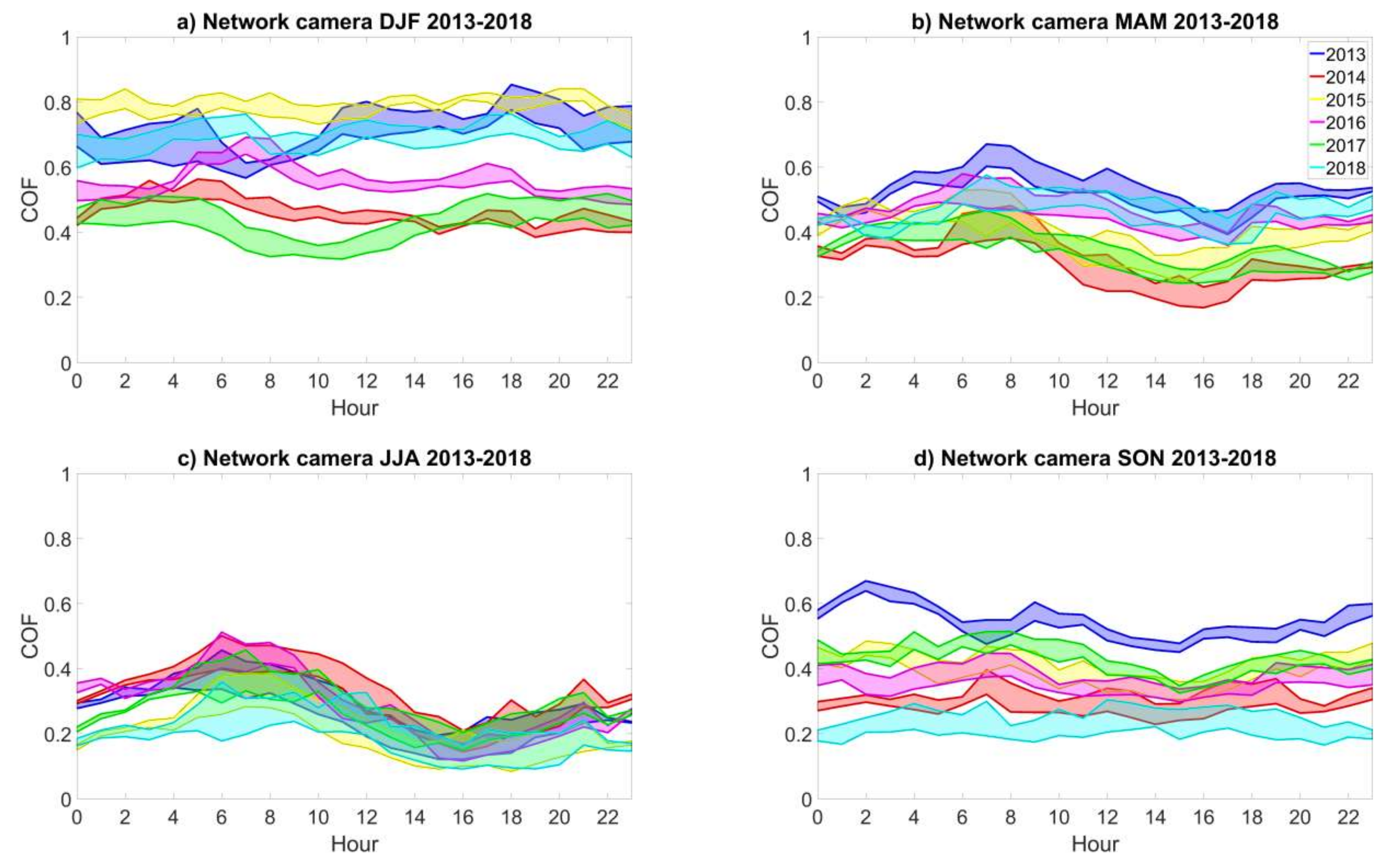
Figure 5 presents the mean COF daily variation separated by seasons and years.
The main climatological features we can address are the following:
- -
There is a clear diurnal cycle during summer, with a larger cloud occurrence from 0 to 11 UT (mean value = 0.30) than from 12 to 23UT (mean value = 0.18), a less pronounced diurnal cycle during spring, and no diurnal cycle observed during winter and autumn. This feature could be linked to the seasonal changes in the day/night contrast of the boundary layer height (BLH), with a higher BLH observed during daytime in summer and spring [
32]. During summer and spring, more daytime clouds may occur above the PUY station and are thus not detected by the camera.
- -
A strong seasonal cycle is observed, with the largest values in winter (mean value = 0.60), followed by spring (mean value = 0.41), autumn (mean value = 0.37), and summer (mean value = 0.24).
- -
The inter-annual variability depends on the season. This value can be estimated by calculating the daily mean of the difference between the maximum value and the minimum value of cloud occurrence. We found the largest inter-annual variability in winter (0.38), then autumn (0.32) and spring (0.23), with the lowest inter-annual variability in summer (0.14). The inter-annual variability does not depend on the hour of the day. The larger variability in winter could be simply due to the fact that there are more clouds in the winter. The low values of cloud cover in 2018 could be linked to the heat wave episode observed in Western Europe.
6. Comparisons with Larger Scale Cloud Parameters
It is interesting to compare the COF calculated from the camera image analysis (which corresponds to a local scale) to other parameters representative of the cloud conditions on a larger scale. In this section, we provide a preliminary comparison between the camera analysis results with different cloud cover parameters on a larger scale, in order to evaluate which product is closest to a local measure. This is also an estimation of how the PUY measurements are representative of larger scale cloud cover (i.e., how the measurements are biased by local orographic cloud formation).
6.1. CATS
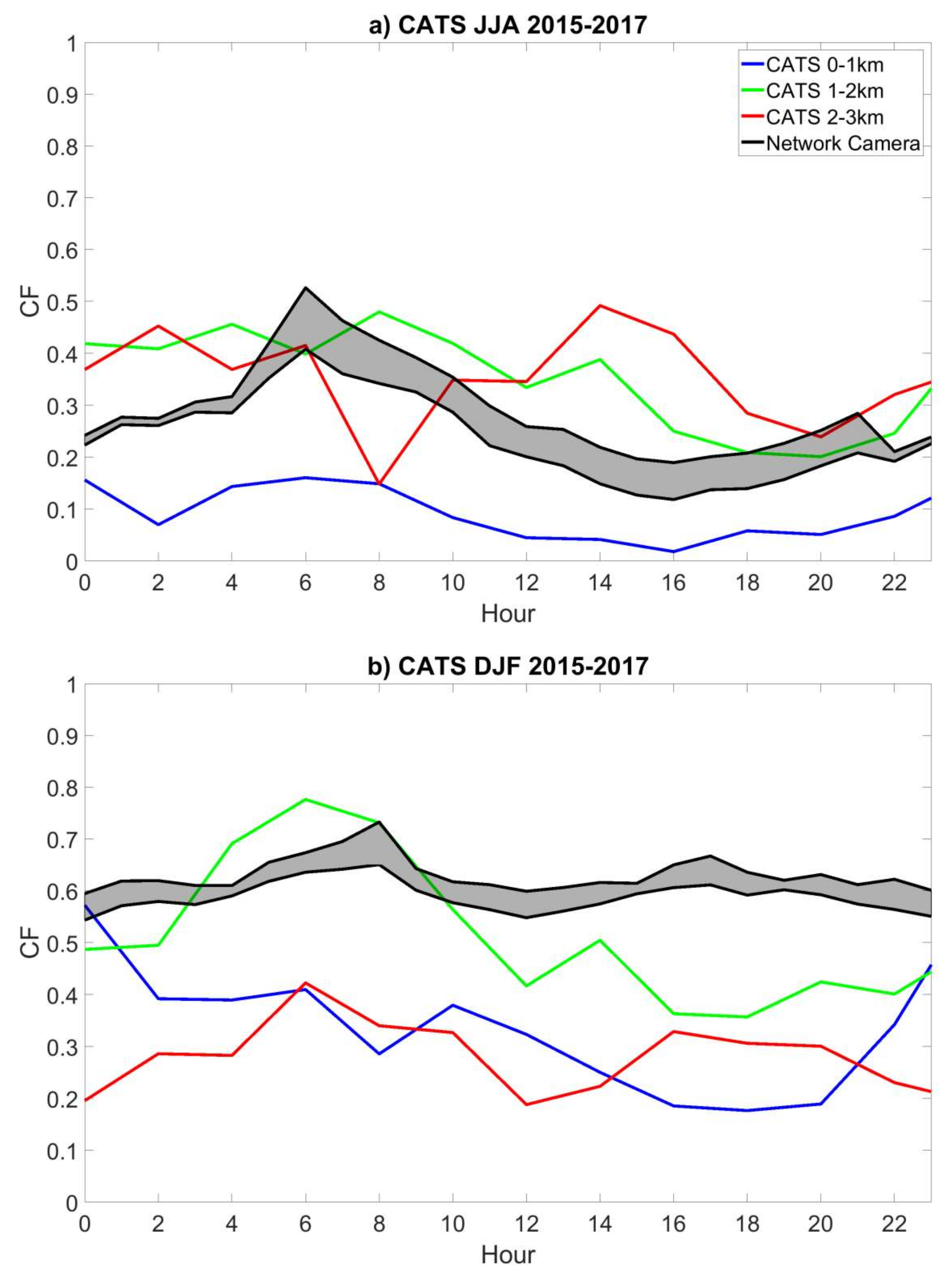
Figure 6 shows the camera COF averaged over the CATS measurement periods (2015–2017), compared to the CF obtained from CATS.
We found that the closest CATS CF values to the camera COF are those of the 1–2 km layer (green curve), which is consistent with the altitude of the PUY roughly in the middle of this altitude range. The results are presented by separating the database into two seasons, summer for the months of June to August (
Figure 6a) and winter for the months of December to February (
Figure 6b). The camera CF is of the same order of magnitude for both types of data, but CATS shows a larger diurnal variation, with CF values larger than the camera cloud occurrence values from 3 to 9 UT during winter and the opposite during the rest of the day. The camera does not show such daily variability during winter; the value of the CF is of the same order of magnitude during night and day (around 0.6). In summer, the daily variability of the CATS CF is less important than in winter, bringing the daily evolution closer to that of the camera. We found that the CF of CATS is, on average, 11% larger than that the camera cloud occurrence. In winter (
Figure 6b), the CATS results show that the CF is largest at the PUY altitude (1–2 km). At higher and lower altitudes, the CF is significantly less. During summertime (
Figure 6a), the CF at lower altitudes falls down to 0.1, while at higher altitudes (1–2 and 2–3 km), the CATS CF is quite similar to the camera COF.
6.2. Meteosat-SEVIRI
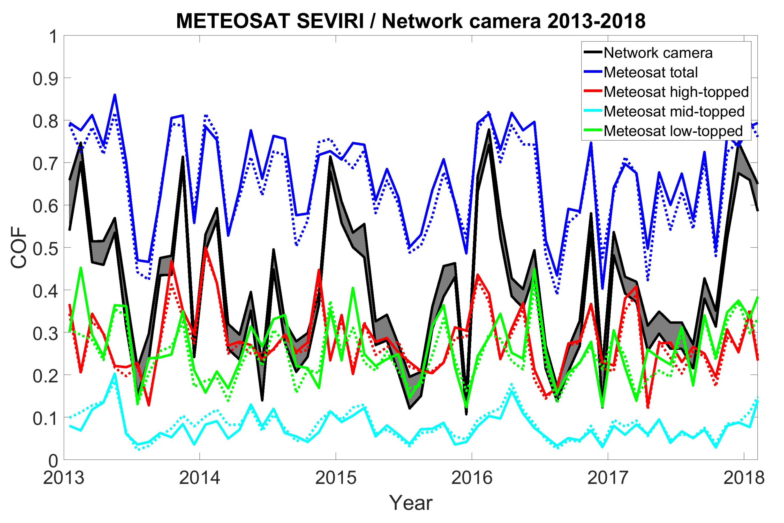
We compared the COF values determined by the camera image analysis with those extracted from METEOSAT SEVIRI on the nearest pixel to PUY and also on a larger area of around 200 km for different vertical levels of the cloud top altitudes (
Figure 7).
The SEVIRI total COF is always larger than the COF deduced from the camera analysis. The difference is 0.25 in average, which probably corresponds to the cases when the cloud base is higher than the altitude of PUY or when the cloud top is lower than the PUY altitude.
The seasonality of COF obtained by the camera analysis (maximum clouds in winter and minimum in summer) is also seen in the METEOSAT-SEVIRI total COF but with a smaller amplitude. For example, the difference between winter and summer on the total COF is only between 0.10 and 0.30. The METEOSAT-SEVIRI low-topped cloud curve is the closest to the camera COF curve (correlation coefficient of 0.60), but the winter maximums are underestimated. In winter, peaks in the webcam COF curve coincide with peaks in the low-topped COF serie but also with peaks in the high-topped COF serie. This is in agreement with the more frequent occurrence of large cloud systems associated with disturbances during this season [
28]. In this large-scale cloud system, thick upper clouds prevent the detection of low clouds with METEOSAT-SEVIRI.
Otherwise, for all altitude levels, the METEOSAT-SEVIRI curve corresponding to the nearest pixel over PUY is close to the curve corresponding to the 200 km domain. This suggests that the small-scale cloud cover around the top of PUY has less influence on the METEOSAT-SEVIRI cloud parameters than large scale cloud cover, regardless of the altitude range.
6.3. All-Sky Camera
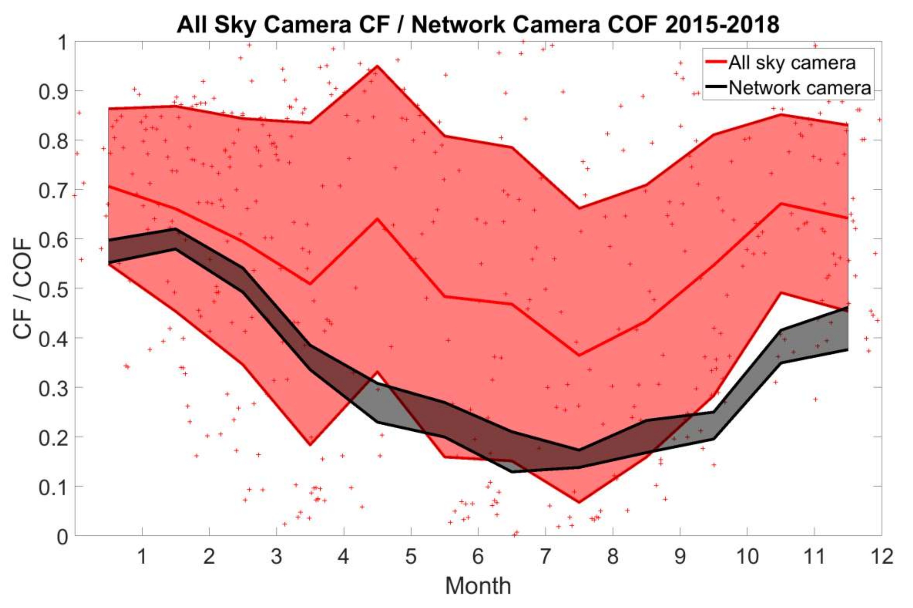
We have also compared the COF deduced from the camera analysis to the CF calculated with the algorithm ELIFAN [
18] applied to the all-sky camera images taken at the Cézeaux site from December 2015 to June 2019 (
Figure 8).
The ELIFAN CF parameter presents larger variability compared to the local camera COF but follows a similar seasonal evolution, with larger mean values in winter (0.67) than in summer (0.44). The all-sky camera CF is determined locally but integrates the cloud cover over a larger area than the cloud occurrence at PUY. In agreement with the results presented in
Section 6.2, the fact that the ELIFAN and camera parameters follow a similar evolution suggests that the COF at PUY is representative of large-scale processes.
6.4. ECMWF ERA-5
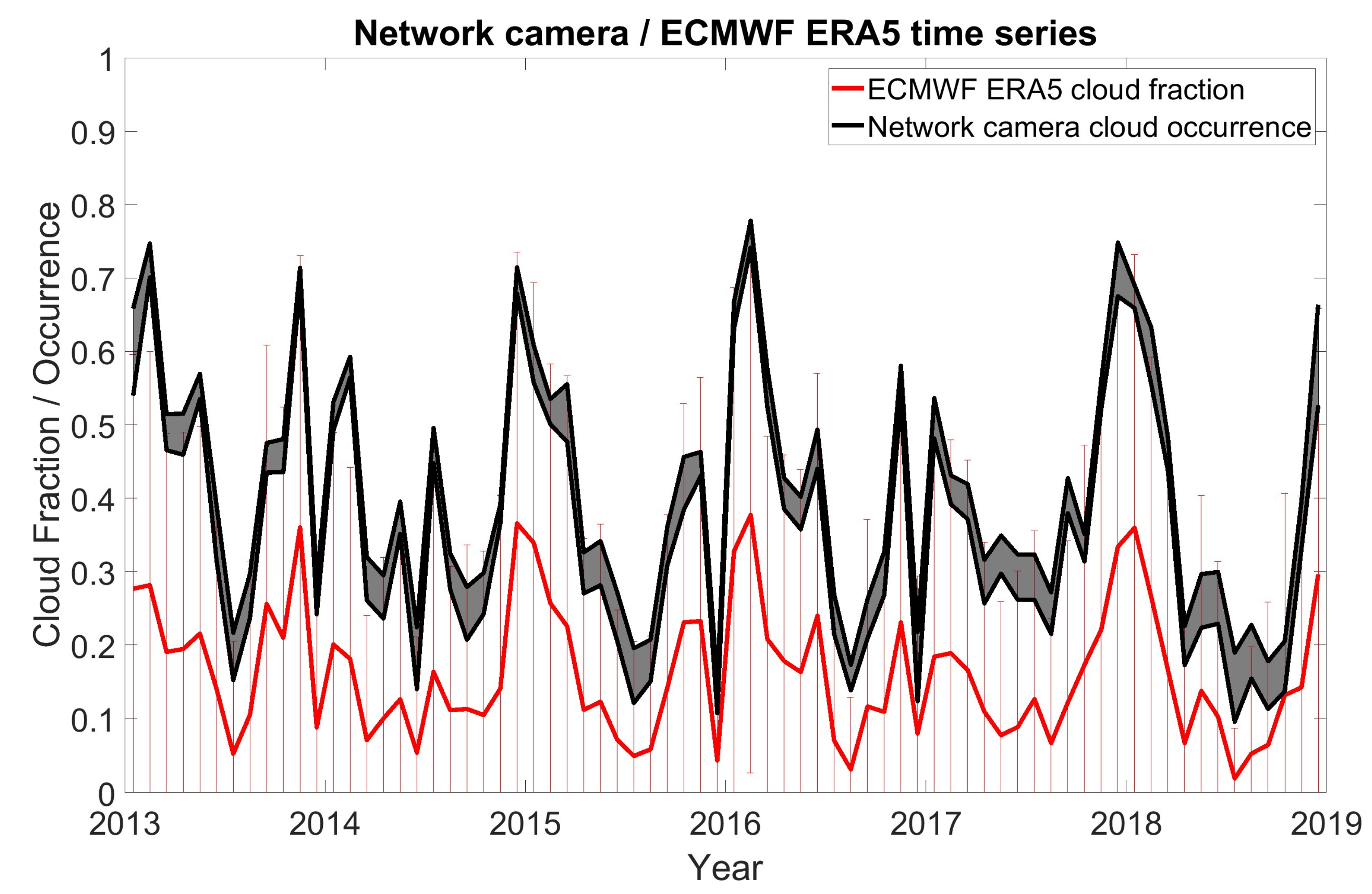
We have also compared the COF deduced from the camera analysis to the fraction of the cloud cover parameter of the ERA-5 dataset recently provided by ECMWF, interpolated on the closest point to PUY at a 850 hPa pressure level.
Figure 9 shows the time series of the monthly averages of these two parameters. The two time series follow highly correlated variations (correlation coefficient 0.94) but with a mean shift of 19% (up to 40% for some winter months). This result suggests that the local cloud cover over a mountain site is probably underestimated by the ECMWF ERA-5 reanalysis. However, the monthly average plus one standard deviation is very close to the COF camera curve.
7. Conclusions
The objective of this work was to show the feasibility of the detection of cloud occurrence on an altitude site from a simple, low-cost, and automatic algorithm based on an analysis of camera images. The comparison of the results of our algorithm with in-situ microphysical data (PVM Gerber) are in good agreement.
The application of this algorithm to the PUY camera over the period 2013–2018 shows that a cloud diurnal cycle is observable only in summer and spring (cloud occurrence is larger during the night than during the day), but this may be because high level daytime clouds during this season are not detected by the camera. There is a strong seasonal cycle with larger values of cloud occurrence in winter than in summer. The inter-annual variability is also high, although it is globally smaller than the seasonal cycle; however, it is also larger in winter than in summer. Specific meteorological conditions could probably explain this inter-annual variability. A more in-depth study of the relationship between the weather conditions and the inter-annual variability of the cloud occurrence frequency could be investigated in the future.
The seasonal variability of clouds was also found from larger scale cloud detection techniques: the all-sky imager located at Cézeaux, 10 km far from PUY, from space observations (CATS, Meteosat), and from global model outputs (ECMWF ERA-5). The one by one comparison of different techniques provides further information on the representativeness of the PUY site.
The comparison with CATS CF shows that, in winter, the CATS CF is of the same order of magnitude as the camera COF, with a larger daily variability for CATS, and, in summer, the daily variability of the CATS CF is less important than in winter, producing daily evolution closer to that of the camera COF. This observation confirms that daytime summertime clouds may develop above the site and are seen by the camera.
A comparison with METEOSAT-SEVIRI products shows that the low-topped COF is the closest parameter to the camera COF, but the winter maximum is underestimated. This is due at least in part to the fact that when high clouds are occurring, low clouds cannot be detected by METEOSAT-SEVIRI.
The comparison with the monthly fraction of cloud cover from the ECMWF ERA-5 reanalysis shows extremely correlated variations (a coefficient correlation of 0.93) but a mean shift of 19%, with larger values for the camera COF than the ECMWF ERA-5 fraction of cloud cover. Despite this shift, the camera COF values remain in the range of ERA-5 +/− one standard deviation.
The CF estimated with the all-sky image at Cézeaux presents a larger variability than the camera COF but follows a similar seasonal evolution, with larger values in winter (0.67) than in summer (0.43). In agreement with the other large scale CF parameters, this suggests that the cloud occurrence PUY is mainly governed by large scale processes.
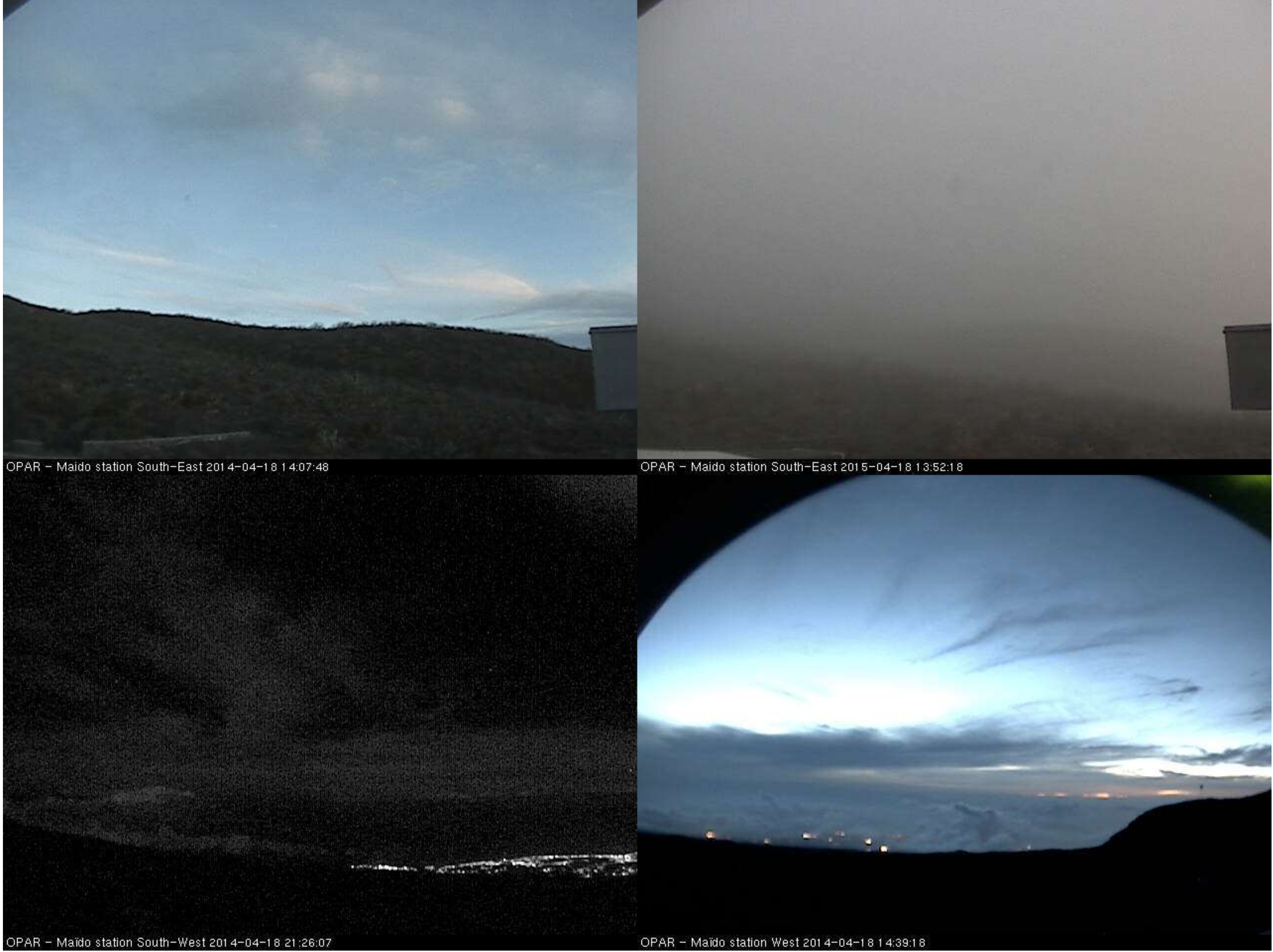
This automatic determination of cloud occurrence is of interest in characterizing observation sites, especially those that are not yet equipped with instruments for the microphysical characterization of clouds. This methodology can also be applied to other high-altitude sites, such as the Maïdo station (Réunion Island, Southern Indian Ocean [
33]), where three cameras oriented toward the west, south-west, and east are in operation (
Figure 10). The application to camera images from other stations would probably need an adaptation of the choice of windows and variability detection thresholds, which depend on the angle of viewing and on the quality of the images.
Another future plan could be to adapt Babari’s method [
34] to calculate atmospheric visibility coefficients from the altitude site cameras in order to classify the cloud occurrence related to the cameras’ opacity.
Few altitude sites are equipped with complex and expensive cloud microphysics instruments, but many are equipped with simple cameras. The application of this method to a sufficient number of sites could be used to quantify the sub-grid variability of cloud cover as seen by most satellites or global models.
Author Contributions
Conceptualization, J.-L.B.; data curation, P.C., J.-M.P., N.M., V.N., and G.S.; formal analysis, J.-L.B., A.B., N.M., V.N., and G.S.; funding acquisition, J.-L.B., L.D., and N.M.; investigation, J.-L.B., A.B., K.S., N.M., V.N., and G.S.; methodology, J.-L.B.; project administration, J.-L.B.; resources, P.C., J.-M.P., N.M.; V.N., G.S.; F.G., and G.P.; software, J.-L.B. and A.B.; supervision, J.-L.B.; validation, J.-L.B.; visualization, J.-L.B.; writing—original draft, J.-L.B.; writing—review and editing, J.-L.B., K.S., L.D., N.M.,V.N., G.S., and V.D.
Funding
This research received no external funding.
Acknowledgments
This study benefited from discussions during the workshops ACTRIS-FR and EECLAT and the seminar given to the laboratory LaMP. Régis Dupuy and Pierre Coutris are acknowledged for suggesting useful references, Sandra Banson for extracting ECMWF ERA 5 reanalysis, and Nicolas Pascal for reprocessing ELIFAN calculations.
Conflicts of Interest
The authors declare no conflict of interest.
References
- Hartmann, D.L.; Doelling, D. On the net radiative effectiveness of clouds. J. Geophys. Res. Atmos. 1991, 96, 869–891. [Google Scholar] [CrossRef]
- Van Baelen, J.; Reverdy, M.; Tridon, F.; Labbouz, L.; Dick, G.; Bender, M.; Hagen, M. On the relationship between water vapour field evolution and the life cycle of precipitation systems. Q. J. R. Meteorol. Soc. 2011, 137, 204–223. [Google Scholar] [CrossRef]
- Bony, S.; Colman, R.; Kattsov, V.M.; Allan, R.P.; Bretherton, C.S.; Dufresne, J.-L.; Hall, A.; Hallegatte, S.; Holland, M.M.; Ingram, W.; et al. How well do we understand and evaluate climate change feedback processes? J. Clim. 2006, 19, 3445–3482. [Google Scholar] [CrossRef]
- Ceppi, P.; Brient, F.; Zelinka, M.D.; Hartmann, D.L. Cloud feedback mechanisms and their representation in global climate models. Wiley Interdiscip. Rev. Clim. Chang. 2017, 8, e465. [Google Scholar] [CrossRef]
- Wallace, J.M.; Hobbs, P.V. 6—Cloud Microphysics. In Atmospheric Science, 2nd ed.; Wallace, J.M., Hobbs, P.V., Eds.; Academic Press: San Diego, CA, USA, 2006; pp. 209–269. ISBN 978-0-12-732951-2. [Google Scholar]
- Renard, P.; Canet, I.; Sancelme, M.; Wirgot, N.; Deguillaume, L.; Delort, A.-M. Screening of cloud microorganisms isolated at the Puy de Dôme (France) station for the production of biosurfactants. Atmos. Chem. Phys. 2016, 16, 12347–12358. [Google Scholar] [CrossRef]
- Köhler, H. The nucleus in and the growth of hygroscopic droplets. Trans. Faraday Soc. 1936, 32, 1152–1161. [Google Scholar] [CrossRef]
- ACTRIS Objectives Webpage. Available online: https://www.actris.eu/About/ACTRIS/Objectives.aspx (accessed on 12 December 2019).
- Guyot, G.; Gourbeyre, C.; Febvre, G.; Shcherbakov, V.; Burnet, F.; Dupont, J.-C.; Sellegri, K.; Jourdan, O. Quantitative evaluation of seven optical sensors for cloud microphysical measurements at the Puy-de-Dôme Observatory, France. Atmos. Meas. Tech. 2015, 8, 4347–4367. [Google Scholar] [CrossRef]
- Deguillaume, L.; Charbouillot, T.; Joly, M.; Vaïtilingom, M.; Parazols, M.; Marinoni, A.; Amato, P.; Delort, A.-M.; Vinatier, V.; Flossmann, A.; et al. Classification of clouds sampled at the puy de Dôme (France) based on 10 yr of monitoring of their physicochemical properties. Atmos. Chem. Phys. 2014, 14, 1485–1506. [Google Scholar] [CrossRef]
- Vaïtilingom, M.; Attard, E.; Gaiani, N.; Sancelme, M.; Deguillaume, L.; Flossmann, A.I.; Amato, P.; Delort, A.-M. Long-term features of cloud microbiology at the puy de Dôme (France). Atmos. Environ. 2012, 56, 88–100. [Google Scholar] [CrossRef]
- Li, J.; Wang, X.; Chen, J.; Zhu, C.; Li, W.; Li, C.; Liu, L.; Xu, C.; Wen, L.; Xue, L.; et al. Chemical composition and droplet size distribution of cloud at the summit of Mount Tai, China. Atmos. Chem. Phys. 2017, 17, 9885–9896. [Google Scholar] [CrossRef]
- Van Pinxteren, D.; Fomba, K.W.; Mertes, S.; Müller, K.; Spindler, G.; Schneider, J.; Lee, T.; Collett, J.L.; Herrmann, H. Cloud water composition during HCCT-2010: Scavenging efficiencies, solute concentrations, and droplet size dependence of inorganic ions and dissolved organic carbon. Atmos. Chem. Phys. 2016, 16, 3185–3205. [Google Scholar] [CrossRef]
- Bianco, A.; Deguillaume, L.; Vaïtilingom, M.; Nicol, E.; Baray, J.-L.; Chaumerliac, N.; Bridoux, M. Molecular Characterization of Cloud Water Samples Collected at the Puy de Dôme (France) by Fourier Transform Ion Cyclotron Resonance Mass Spectrometry. Environ. Sci. Technol. 2018, 52, 10275–10285. [Google Scholar] [CrossRef] [PubMed]
- Baray, J.-L.; Deguillaume, L.; Colomb, A.; Sellegri, K.; Freney, E.; Rose, C.; Van Baelen, J.; Pichon, J.-M.; Picard, D.; Fréville, P.; et al. Cézeaux-Aulnat-Opme-Puy De Dôme: A multi-site for the long term survey of the tropospheric composition and climate change. Atmos. Meas. Tech. Discuss. 2019. [Google Scholar] [CrossRef]
- Axis Webpage. Available online: https://www.axis.com/en (accessed on 12 December 2019).
- OPGC Webcam Page. Available online: http://wwwobs.univ-bpclermont.fr/opgc/webcam.php (accessed on 12 December 2019).
- Lothon, M.; Barnéoud, P.; Gabella, O.; Lohou, F.; Derrien, S.; Rondi, S.; Chiriaco, M.; Bastin, S.; Dupont, J.-C.; Haeffelin, M.; et al. ELIFAN, an algorithm for the estimation of cloud cover from sky imagers. Atmos. Meas. Tech. 2019, 12, 5519–5534. [Google Scholar] [CrossRef]
- Gerber, H. Liquid water content of fogs and hazes from visible light scattering. J. Clim. Appl. Meteorol. 1984, 23, 1247–1252. [Google Scholar] [CrossRef]
- Gerber, H. Direct measurement of suspended particulate volume concentration and far-infrared extinction coefficient with a laser-diffraction instrument. Appl. Opt. 1991, 30, 4824–4831. [Google Scholar] [CrossRef]
- McGill, M.J.; Yorks, J.E.; Scott, V.S.; Kupchock, A.W.; Selmer, P.A. The Cloud-Aerosol Transport System (CATS): A technology demonstration on the International Space Station. Lidar Remote Sens. Environ. Monit. 2015, 96, 1–6. [Google Scholar]
- Pauly, R.M.; Yorks, J.E.; Hlavka, D.L.; McGill, M.J.; Amiridis, V.; Palm, S.P.; Rodier, S.D.; Vaughan, M.A.; Selmer, P.A.; Kupchock, A.W.; et al. Cloud Aerosol Transport System (CATS) 1064 nm calibration and validation. Atmos. Meas. Tech. Discuss. 2019, 12, 6241–6258. [Google Scholar] [CrossRef]
- Noel, V.; Chepfer, H.; Chiriaco, M.; Yorks, J. The diurnal cycle of cloud profiles over land and ocean between 51° S and 51° N, seen by the CATS spaceborne lidar from the International Space Station. Atmos. Chem. Phys. 2018, 18, 9457–9473. [Google Scholar] [CrossRef]
- Data Product Catalog Release 3.0. Available online: https://cats.gsfc.nasa.gov/media/docs/CATS_Data_Products_Catalog.pdf (accessed on 12 December 2019).
- EUMETSAT NWC SAF Homepage. Available online: http://www.nwcsaf.org/ (accessed on 12 December 2019).
- Derrien, M.; Le Gléau, H. MSG/SEVIRI cloud mask and type from SAFNWC. Int. J. Remote Sens. 2005, 26, 4707–4732. [Google Scholar] [CrossRef]
- Derrien, M.; Le Gléau, H. Improvement of cloud detection near sunrise and sunset by temporal-differencing and region-growing techniques with real-time SEVIRI. Int. J. Remote Sens. 2010, 31, 1765–1780. [Google Scholar] [CrossRef]
- Sèze, G.; Pelon, J.; Derrien, M.; Le Gléau, H.; Six, B. Evaluation against CALIPSO lidar observations of the multi-geostationary cloud cover and type dataset assembled in the framework of the Megha-Tropiques mission. Q. J. R. Meteorol. Soc. 2015, 141, 774–797. [Google Scholar] [CrossRef]
- Albergel, C.; Dutra, E.; Munier, S.; Calvet, J.-C.; Munoz-Sabater, J.; de Rosnay, P.; Balsamo, G. ERA-5 and ERA-Interim driven ISBA land surface model simulations: Which one performs better? Hydrol. Earth Syst. Sci. 2018, 22, 3515–3532. [Google Scholar] [CrossRef]
- Matlab Mathworks Homepage. Available online: https://www.mathworks.com/products/matlab.html (accessed on 12 December 2019).
- Python Homepage. Available online: https://www.python.org (accessed on 12 December 2019).
- Farah, A.; Freney, E.; Chauvigné, A.; Baray, J.-L.; Rose, C.; Picard, D.; Colomb, A.; Hadad, D.; Abboud, M.; Farah, W.; et al. Seasonal variation of aerosol size distribution data at the puy de Dôme station with emphasis on the boundary layer/free troposphere segregation. Atmosphere 2018, 9, 244. [Google Scholar] [CrossRef]
- Baray, J.-L.; Courcoux, Y.; Keckhut, P.; Portafaix, T.; Tulet, P.; Cammas, J.-P.; Hauchecorne, A.; Godin Beekmann, S.; De Mazière, M.; Hermans, C.; et al. Maïdo observatory: A new high-altitude station facility at Reunion Island (21° S, 55° E) for long-term atmospheric remote sensing and in situ measurements. Atmos. Meas. Tech. 2013, 6, 2865–2877. [Google Scholar] [CrossRef]
- Babari, R.; Hautière, N.; Dumont, É.; Paparoditis, N.; Misener, J. Visibility monitoring using conventional roadside cameras—Emerging applications. Transp. Res. Part C Emerg. Technol. 2012, 22, 17–28. [Google Scholar] [CrossRef]
Figure 1.
Geographical configuration and fields of view of the network cameras in operation at Cézeaux and puy de Dôme station (PUY) sites superimposed to a ©Google Map image (top) and photographs of the PUY platform hosting the network camera (bottom left), PVM Gerber (bottom center), and the EKO all-sky imager on the Cézeaux site (bottom right). A camera similar to the one in operation at PUY is also in operation of the Cézeaux site (not used in this work) but is not visible in the photo.
Figure 2.
Examples of images and MATLAB processing outputs for different situations, from top to bottom: night time clear sky, day-time clear sky, night-time sea of clouds, and day-time cloud. The two zones are indicated with black rectangles, and the days and hours and standard deviation values in the two areas of Clermont (bottom large rectangle) and Livradois-Forez (top little rectangle) are given on the top of each image.
Figure 3.
(a) Percentage of the agreement between cloud occurrence from the particulate volume monitor (PVM) and camera depending on the threshold values of the camera data processing (Clermont on the X axis, Livradois Forez on the y axis). (b) The same plot reduced for daytime images (9 to 16 UT). (c) Same plot reduced for nighttime images (23 to 4 UT).
Figure 4.
(a) Cloud occurrence frequency (COF) monthly time series calculated from camera images in black, with PVM Gerber in red. The lower limit of the camera curve is obtained with the threshold value 5.5, and the upper limit is obtained by adding the cases classified as “uncertain” with threshold values between 5.5 and 6.5. The PVM Gerber points with less than 30% of validated available data have been removed, and the PVM Gerber points with more than 30% and 70% are in red and blue, respectively. (b) A scatterplot of the monthly cloud occurrence from the camera images (threshold value at 6) as a function of PVM Gerber. The color is the percentage of validated PVM Gerber data per month, and the line y = x is in black.
Figure 5.
(
a) Network camera DJF 2013-2018; (
b) Network camera MAM 2013-2018; (
c) Network camera JJA 2013-2018; (
d) Network camera SON 2013-2018. COF obtained from the camera image processing separated by seasons and years as a function of the hours of the day (UTC). For each year and season, the uncertainty interval has been estimated similarly to
Figure 4a. The correspondence between the colors and years is given in the top-right corner.
Figure 6.
CF as function of time of the day (UT), extracted from the cloud-aerosol transport system (CATS) in summer 2015–2017 (a) and winter 2015–2017 (b) for three vertical ranges above sea level, 0–1 km in blue, 1–2 km in green, and 2–3 km in red, compared to the COF deduced from the PUY camera in black. The sea cloud camera situations have been added to the cloud situation for this comparison. The lower limit of the camera cloud occurrence (black curve) is obtained with a threshold value of 5.5, and the upper limit is obtained by adding the cases classified as “uncertain” (with a threshold value between 5.5 and 6.5).
Figure 7.
Total, high-topped, mid-topped, and low-topped COF (in blue, red, cyan, and green, respectively), extracted from METEOSAT-SEVIRI on the nearest pixel over PUY (continuous lines), as well as on a larger region between 44.6 and 46.9° N and between 2 and 4° E (dashed lines), compared to the monthly mean of the camera COF in black.
Figure 8.
Daily (red crosses) and monthly +/− one sigma (red lines) means of the CF calculated with the algorithm ELIFAN applied to the all-sky camera images taken at the Cézeaux site from December 2015 to June 2019, compared to the monthly mean of the COF from the camera analysis in black.
Figure 8.
Daily (red crosses) and monthly +/− one sigma (red lines) means of the CF calculated with the algorithm ELIFAN applied to the all-sky camera images taken at the Cézeaux site from December 2015 to June 2019, compared to the monthly mean of the COF from the camera analysis in black.
Figure 9.
Time series of the monthly mean and standard deviation of the ERA 5 ECMWF fraction of the cloud cover interpolated on the point 45.77° N, 2.95° E on the 850 hPa pressure level in red, compared to the monthly mean of the camera COF in black.
Figure 9.
Time series of the monthly mean and standard deviation of the ERA 5 ECMWF fraction of the cloud cover interpolated on the point 45.77° N, 2.95° E on the 850 hPa pressure level in red, compared to the monthly mean of the camera COF in black.
Figure 10.
Examples of images of a camera in operation at Maïdo station (Réunion Island, 2160 m above the sea level, towards the south-east—clear sky and cloudy (top), and towards the south west during night and day (bottom), where the algorithm of detection of the CF could be applied in the future.
Table 1.
The percentage of available network camera images at PUY related to the maximum number of images theoretically available per month (lines) and year (columns).
Table 1.
The percentage of available network camera images at PUY related to the maximum number of images theoretically available per month (lines) and year (columns).
| Month | 2013 | 2014 | 2015 | 2016 | 2017 | 2018 |
|---|
| January | 99.3% | 87.6% | 90.6% | 93.9% | 94.0% | 100% |
| February | 100% | 99.3% | 76.1% | 99.9% | 100% | 95.1% |
| March | 92.1% | 99.4% | 95.8% | 98.7% | 99.0% | 99.9% |
| April | 98.7% | 100% | 97.8% | 97.6% | 100% | 97.0% |
| May | 92.9% | 99.7% | 92.5% | 94.9% | 99.9% | 55.5% |
| June | 98.6% | 98.5% | 88.2% | 90.9% | 100% | 99.7% |
| July | 97.4% | 97.4% | 96.2% | 92.3% | 96.8% | 96.7% |
| August | 95.8% | 99.7% | 86.1% | 96.6% | 96.3% | 94.1% |
| September | 98.3% | 96.3% | 92.8% | 98.7% | 99.6% | 97.6% |
| October | 96.0% | 98.6% | 96.4% | 99.5% | 98.1% | 82.9% |
| November | 92.2% | 95.1% | 100% | 95.8% | 100% | 100% |
| December | 88.7% | 72.5% | 97.1% | 89.9% | 100% | 98.0% |
Table 2.
Monthly data during 2013–2018 and the correlation coefficients after removing the months when PVM Gerber was working less than the different thresholds from 30% to 90%.
Table 2.
Monthly data during 2013–2018 and the correlation coefficients after removing the months when PVM Gerber was working less than the different thresholds from 30% to 90%.
| PVM Gerber Working More than | Number of Monthly Points | Correlation Coefficient |
|---|
| 0% (The whole serie) | 72 | 0.46 |
| 30% | 59 | 0.53 |
| 40% | 57 | 0.55 |
| 50% | 53 | 0.65 |
| 60% | 49 | 0.73 |
| 70% | 41 | 0.82 |
| 80% | 37 | 0.89 |
| 90% | 31 | 0.92 |
© 2019 by the authors. Licensee MDPI, Basel, Switzerland. This article is an open access article distributed under the terms and conditions of the Creative Commons Attribution (CC BY) license (http://creativecommons.org/licenses/by/4.0/).

 ,
, 


