Article

North American Winter Dipole: Observed and Simulated Changes in Circulations

by
Yu-Tang Chien
1,†,
S.-Y. Simon Wang
1,
Yoshimitsu Chikamoto
1,
Steve L. Voelker
1,‡,
Jonathan D. D. Meyer
1 and
Jin-Ho Yoon
2,*
1
Department of Plants, Soils and Climate/Utah Climate Center, Utah State University, Logan, UT 84322, USA
2
School of Earth Sciences and Environmental Engineering, Gwangju Institute of Science and Technology, Gwangju 61005, Korea
*
Author to whom correspondence should be addressed.
Current affiliation: National Science and Technology Center for Disaster Reduction, New Taipei City 23143, Taiwan.
Current affiliation: Department of Environmental and Forest Biology, SUNY-ESF, Syracuse, NY 13210, USA.
Atmosphere 2019, 10(12), 793; https://doi.org/10.3390/atmos10120793
Submission received: 17 October 2019 / Revised: 26 November 2019 / Accepted: 30 November 2019 / Published: 7 December 2019
(This article belongs to the Special Issue The Impacts of Climate Change on Atmospheric Circulations)

Abstract

:
In recent years, a pair of large-scale circulation patterns consisting of an anomalous ridge over northwestern North America and trough over northeastern North America was found to accompany extreme winter weather events such as the 2013–2015 California drought and eastern U.S. cold outbreaks. Referred to as the North American winter dipole (NAWD), previous studies have found both a marked natural variability and a warming-induced amplification trend in the NAWD. In this study, we utilized multiple global reanalysis datasets and existing climate model simulations to examine the variability of the winter planetary wave patterns over North America and to better understand how it is likely to change in the future. We compared between pre- and post-1980 periods to identify changes to the circulation variations based on empirical analysis. It was found that the leading pattern of the winter planetary waves has changed, from the Pacific–North America (PNA) mode to a spatially shifted mode such as NAWD. Further, the potential influence of global warming on NAWD was examined using multiple climate model simulations.

1. Introduction

Cold-air intrusion events in eastern North America are common during boreal winter, but severe events, with costly consequences, used to be rare. According to the National Centers for Environmental Information report (NOAA 2019) [1], during 1985–2005, Florida was the only state suffering billion-dollar losses related to freeze events. After 2006, the number of eastern states experiencing billion-dollar freeze-related disasters has increased threefold. This trend is concurrent with a marked increase in the number of billion-dollar drought disasters in western states. The exceptionally dry conditions in the 2013–2014 winter and the associated high-amplitude atmospheric ridge in the Northeast Pacific was accompanied by an abnormally deepened trough in the eastern USA with strong cold-air outbreaks. This striking division of severe drought in the west and extreme cold in the east has been referred to as the “North American Winter Temperature Dipole” (Singh et al., 2016) [2], while its accompanying circulation pattern is called the “North American Winter Dipole” (NAWD) (Wang et al., 2015) [3].
The polarity and location of this circulation NAWD coincide with the wintertime stationary waves over North America, which feature a high-pressure ridge in the west and a low-pressure trough in the east (Wang et al., 2017, Stuivenvolt Allen and Wang, 2019) [4,5]. Oscillating in sync with the stationary waves, the positive-phase NAWD is associated with an anomalous ridge over the Gulf of Alaska and a deepened trough near the Great Lakes, thereby enhancing the east–west temperature contrast in North America including prolonged freezing in the Great Lakes (Voelker et al., 2019) [6]. Past studies suggested that the ridge in the western U.S. (Swain et al., 2014) [7] and the temperature dipole itself have amplified (Singh et al., 2016) [2], owing to internal and external variabilities such as tropical Pacific heating (Hartmann 2015; Schulte and Lee 2017) [8,9] and Arctic warming (Francis and Varus 2012; Overland et al., 2016) [10,11]. The intense reversal of NAWD seen in the winter of 2016–2017 and associated extreme precipitation in California suggests that the NAWD variability has also increased (Wang et al., 2017; Swain et al., 2018; Yoon et al., 2015) [4,12,13].
This study explored the wintertime leading pattern evolution across North America and sought to identify potential forcing sources through diagnostic analyses. While the 2013/2014 extreme NAWD event has been extensively studied, the role of large-scale climate variability in terms of the wintertime stationary waves has not been satisfactorily addressed. The overarching goal here was to examine the dominant patterns during the recent decades and to compare that with the known dominant climate mode, including the Pacific–North American (PNA) pattern. Given the reportedly weak correlation between the PNA and NAWD (Wang et. al., 2014; Yoon et al., 2015) [13,14], the two phenomena may be independent and their collective changes in amplitude over time deserves research attention.
In this study, multiple global reanalysis and observational datasets were used alongside global climate model simulations, which are introduced in Section 2. In Section 3, we provide discussions of the analysis results. Concluding remarks are presented in Section 4.

2. Data Sources

2.1. Observations

The primary dataset used to study the atmospheric circulation features of interest is the NCEP–NCAR reanalysis (Kalnay et al., 1996) [15] from 1948 to the present, given its consistent data assimilation utilized throughout the entire period. Although satellite data were lacking before 1979, the temporal coverage of this reanalysis is longer than newer reanalysis that ingests satellite data. We also used European Centre for Medium-Range Weather Forecasts (ECMWF) interim reanalysis (ERA-Interim; Dee et al., 2011) [16] from 1979 to 2015 and extend back to 1958 by concatenating with ERA-40 (Uppala et al., 2005) [17]. Additionally, we used a retrospective reanalysis dataset to depict the global atmospheric circulation: the ECMWF global reanalysis products for the twentieth century (ERA-20C) (Poli et al., 2016) [18] from 1871 to 2012 and the National Oceanic and Atmospheric Administration (NOAA) 20-Century Reanalysis data. Based on large ensembles, 20CR (ERA-20C) utilized a coupled Atmosphere/Land-surface/Ocean model to assimilate surface observations of sea level pressure (surface pressure) to produce the atmospheric conditions. It should be noted that the 20CR dataset is developed from the model simulation forced by surface conditions only; therefore, it is not a full reanalysis. In this study, we utilized the monthly mean North Hemisphere geopotential height from November to February on 2.5° × 2.5° long grid spacing. Regarding sea surface temperature (SST), NOAA Extended Reconstructed Sea Surface Temperature (ERSST) V4 dataset was used in this study, starting in 1854 with a 2° × 2° spatial resolution (Huang et al., 2014) [19].

2.2. Simulations

Model simulation outputs were analyzed from two sources: (1) the Community Earth System Model version 1 (CESM1) Large-Ensemble Project with 40 members (Kay et al., 2015) [20] from 1950 to 2005 for the historical period and from 2040 to 2080 for the projected perspectives driven by Representative Concentration Pathways (RCP) 8.5 scenario; and (2) the 21,000-year-long Paleoclimate simulation from 21,000 years before present (1950 A.D.) produced by the model ECBilt-CLIO, which was forced with time-dependent ice-sheet topography, orbital forcing, and greenhouse gas forcing. Based on a quasi-geostrophic adiabatic core with T21 resolution (64 points for longitude and 32 points for latitude) and three vertical layers (200 mb, 500 mb, and 800 mb), the ECBilt-CLIO includes the prognostic vorticity equation and the thermodynamic equation with a set of physical parameterizations of diabatic processes and coupled with an ocean model. The Paleoclimate simulation started from a 2000-year-long Last Glacial Maximum equilibrium simulation with pre-industrial greenhouse gases. Here, the geopotential height is only available at 500 mb for wintertime (DJF) means.

2.3. NAWD-Related Climate Indices

We further considered a number of documented large-scale climate oscillation indices that were linked to the significant 2013/2014 and 2014/2015 winter anomalies in North America (Table 1). Western North Pacific (WNP) is defined as a specific SSTA pattern that forms one year before a full-fledged El Nino/La Nina, with a growing connection between the WNP pattern and the development of El Niño–Southern Oscillation (ENSO) in the following year since 1960 (Pegion and Selman 2017) [21]. By using the Niño 4 index in the year prior an ENSO event, denoted as Nino4 (Y + 1) fluctuation, Wang et al. (2014) [13] found a close association of the NAWD index with Nino4 (Y + 1). Next, the Blob index describes the Pacific warm water patch in the northeast Pacific during the 2014/2015 California drought event (Bond et al., 2015) [22] owing to the anomalous high-pressure system that works against the prevailing surface westerlies and subsequent reduction in local surface evaporation. Further, Lorenzo and Mantua (2016) [23] identified the Gulf of Alaska (GOA) SST anomaly as an index to depict warming in the Pacific coastal boundary of North America. Schulte and Lee (2017) [9] proposed the East Pacific/North Pacific (EP/NP) pattern citing its relationship with USA temperature variability since the 1950s. The Arctic influence was also considered in the 2013–2014 winter event, when the Arctic Oscillation (AO) reached a strong positive phase (Wang et al., 2014) [13] and apparently affected the eastern and southern part of the US (Lorenzo and Mantua 2016). Finally, we follow Singh et al.’s (2016) definition of the North American Winter Temperature Dipole index by computing the difference of surface temperature between the western and eastern USA. All these indices were documented to have certain connection with the extreme 2013–2014 winter anomalies, representing many processes that involve air–sea interaction and internal climate variability (Table 1).
For the index of NAWD, we followed Wang et al. (2017) [4] by subtracting the monthly anomalies of geopotential height at 250 hPa values between the ridge and trough centers from the 5° × 5° domain averages centered at (53° W, 54° N) and (103° W, 63° N), respectively, to depict the standing pattern of the upper-level circulations that is in-phase with the winter stationary waves. Note that the NAWD index in the paleoclimate simulation data differed from the reanalysis because of discrepancy of the vertical level. To make these data comparable, we used least squares regression, where the NAWD index from the 20CR reanalysis dataset was the independent variable and the NAWD index from the paleoclimate dataset was the dependent variable, computed over the overlapping time period of 1950–1981 for the two datasets.

3. Long-Term Change in Leading Circulation Pattern across North America

To depict the stationary eddies, we computed monthly anomalies of geopotential height (Z) at 250 hPa from November to February, with zonal means removed, herein Δ Z E 250. We then subjected the Empirical orthogonal function (EOF) to running 30-year period of Δ Z E 250, in which each EOF analysis contained 120 realizations (30 years × 4 months), covering the Northern Hemisphere. This month-by-month arrangement of Δ Z E 250 reflects the sub-seasonal variability of winter climate anomalies, which is robust over North America and North Pacific (Higgins et al., 2000) [24]. NCEP–NCAR reanalysis was used as the initial analysis of Δ Z E 250.
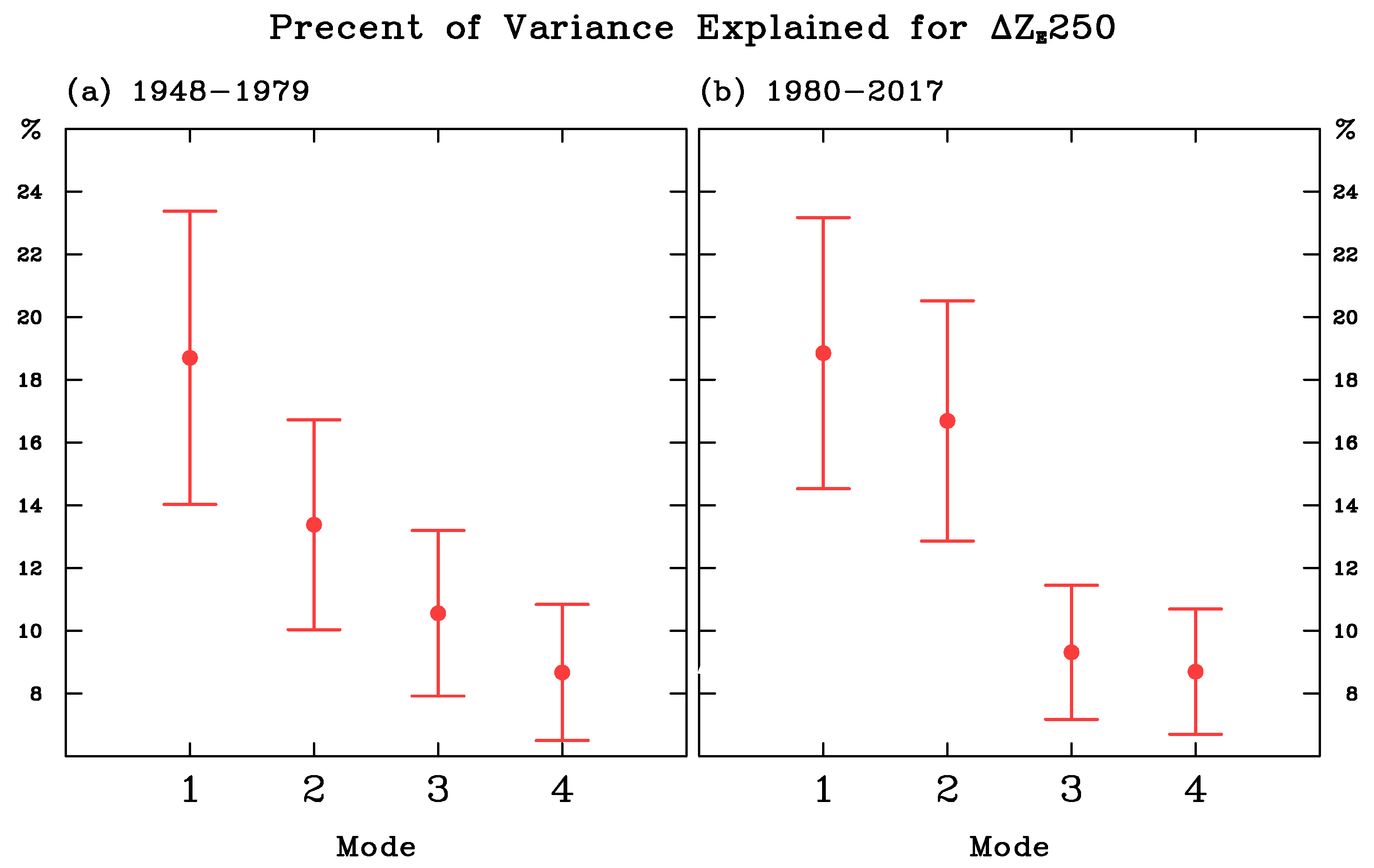
By equally dividing the 1948–2018 period, we set 1980 as the mid-point to distinguish whether circulation patterns have changed. The first EOF mode of Δ Z E 250 during the earlier period (1948–1979) is shown in Figure 1a, explaining 18.6% of the variance. This EOF mode features a wave train emanating from the central Pacific to the U.S. and is coincident with the PNA pattern, which is consistent with the literature (Horel and Wallace 1980) [25]. By superimposing PNA contours (produced by correlating Δ Z E 250 with the PNA index from the NOAA Climate Prediction Center), both EOF1 and PNA patterns are spatially in-phase. By comparison, the post-1980 EOF1 (Figure 1b shading) shows a wave train of similar extent, but the wave centers are shifted from the PNA pattern by a quarter phase. It appears that the post-1980 EOF1 becomes phase-coincident with the NAWD centers marked with × and + in North America. This result suggests that the leading mode of Δ Z E 250 variability may have changed, from a PNA-dominant pattern to one that resembles NAWD. We further tested the rule of thumb provided by North et al. [26] for determining the eigenvalue with an approximate 95% confidence interval. Figure 2 shows the variance of the four modes for each period. The gap between the first and second modes in the early period is greater than in the late period, suggesting that the PNA was initially the dominant driver with a shift toward the NAWD becoming more of a factor (or at least as important as the PNA) in recent decades.
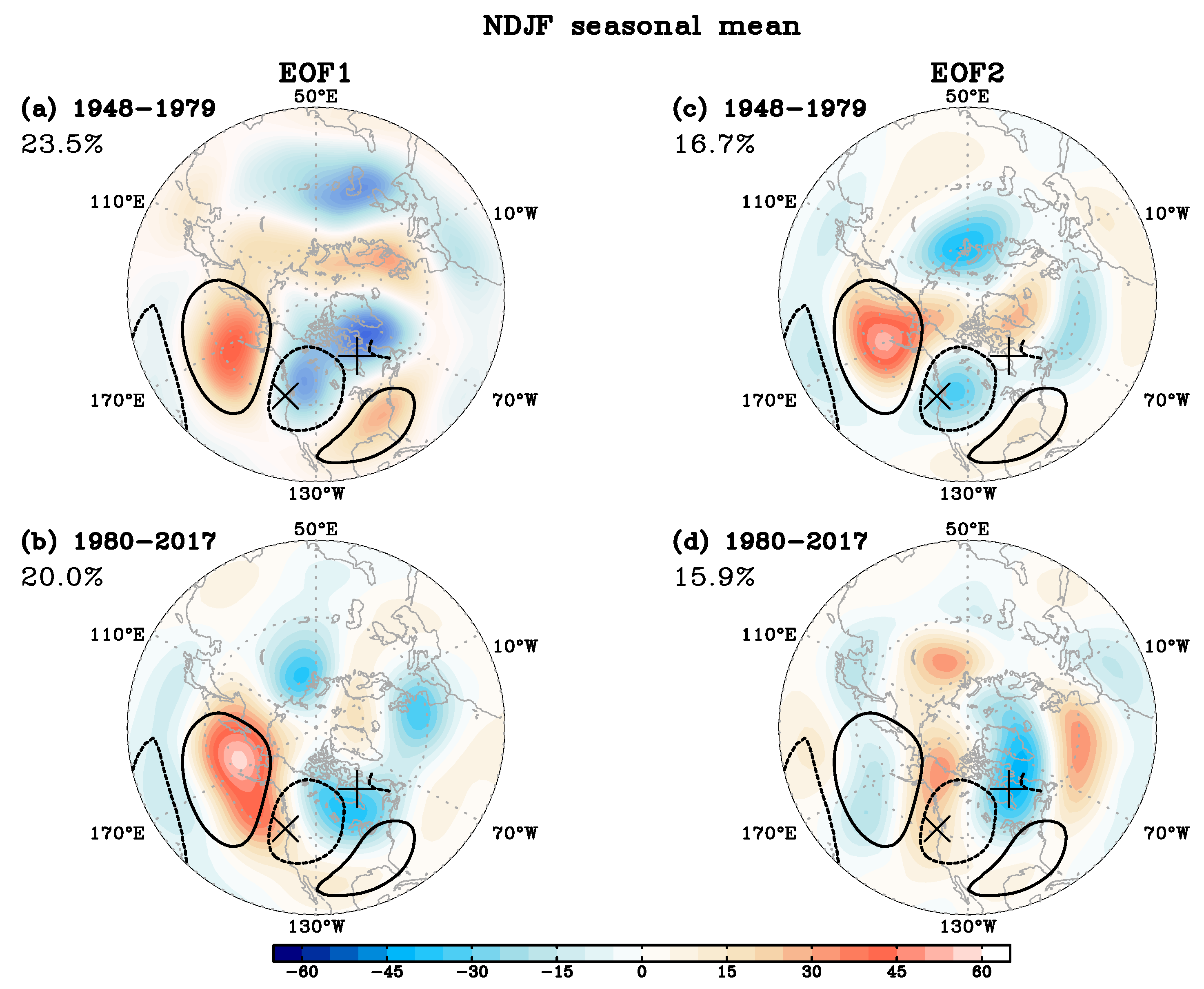
We note that, when applying EOF analysis on seasonal means (Nov-Feb average; Figure 3) instead of monthly intervals, the latter period’s EOF1 remains similar to the PNA (Figure 3b), whereas NAWD lies closer to the second mode (Figure 3d). These results imply that the transition of the leading mode from PNA to NAWD is related to sub-seasonal variability, an emerging subject of intense research (National Academies of Sciences, Engineering, and Medicine. 2016). However, we also note that EOF2 of the earlier period did not reveal the NAWD pattern (Figure 3c), suggesting that its seasonal mode has grown stronger nonetheless in recent decades.
To delineate possible oceanic influences on these leading modes of atmospheric circulation variability, we correlated the first principal component (PC1) time series with monthly SST anomalies (Nov-Feb). As shown in Figure 1c, the pre-1980 EOF1 corresponds to a broad La Niña-like pattern resembling the cold-phase of the Pacific Decadal Oscillation (PDO). After 1980, the PC1 correlation pattern of SST changed dramatically, absent the PDO features alongside most of the tropical signatures (Figure 1d). This post-1980 SST pattern of PC1 reveals the oceanic “blob” along the US West Coast (Kintisch 2015) [27] and robust negative anomalies in the far end of the Western North Pacific and Bay of Bengal. This latter SST feature coincides with an emerging ENSO precursor, called the Western North Pacific pattern (WNP; Wang et al. 2012) [28], that saw an increased association with ENSO development in the following winter during recent decades (Wang et al., 2013; Capotondi and Sardeshmukh 2015) [29,30]. Marked difference between these SST patterns accompanying EOF1 (Δ Z E 250) of the two periods delineates two distinct modes of subtropical variability that influences North American winter climate. These factors are discussed further in Section 3.3.

3.1. Evolution of Pattern Change

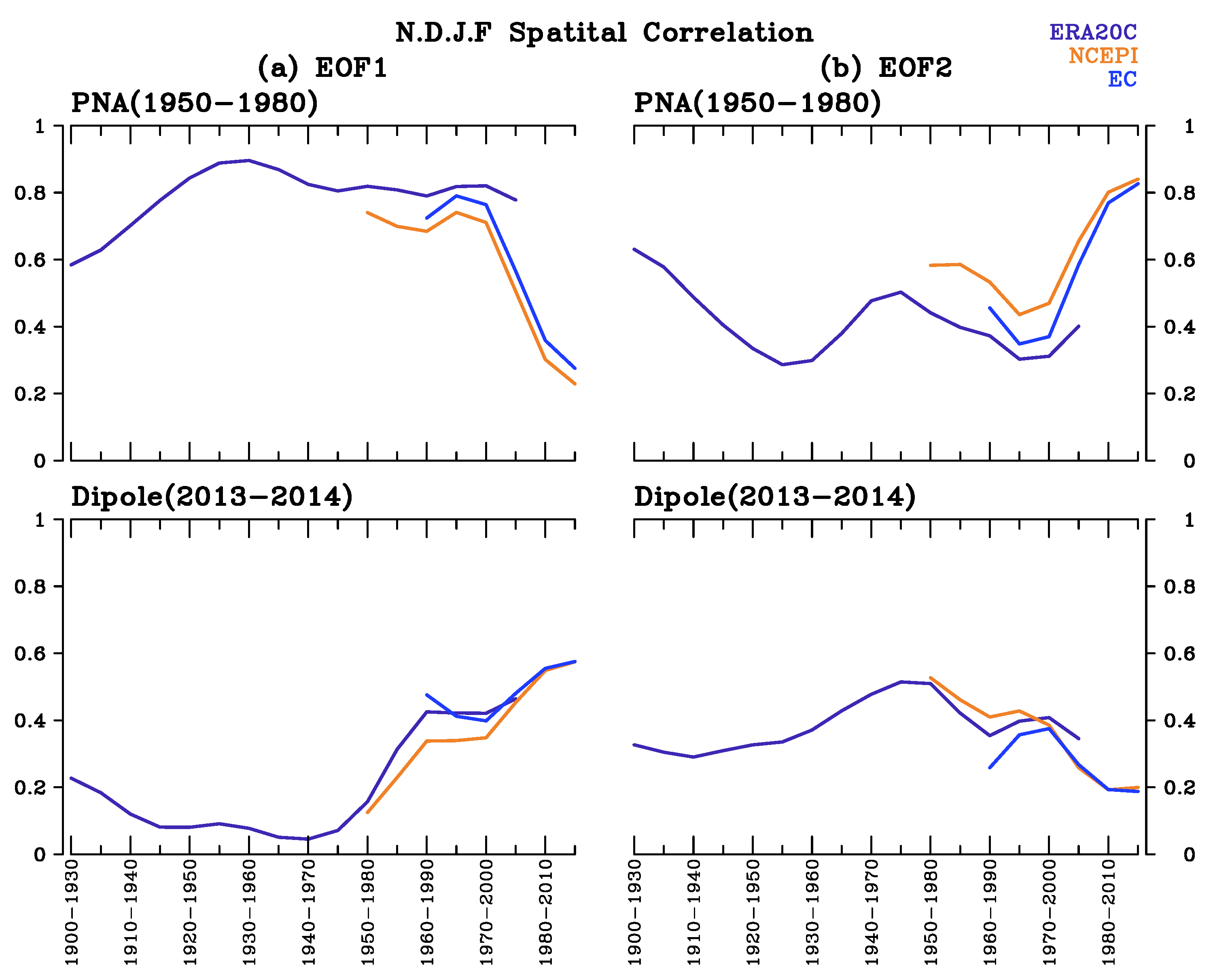
It is important to examine the timing in which the leading mode of Δ Z E 250 started to change. Adopting the running-EOF method of Zhang et al. (2008) [31], a series of EOF analysis was conducted with a 30-year window and repeated every five years. The leading EOFs were then subjected to spatial correlation analyses with the PNA and NAWD patterns, thus forming a series of correlation coefficients from each 30-year period. To validate the NCEP–NCAR reanalysis, these analyses were performed on the ERA20C and the ERA-Interim as well. As shown in Figure 4a, the running-EOFs of all three reanalysis datasets reveal a decreasing trend in the correlations between EOF1 and PNA from 1970 to 2000; meanwhile, the correlations increased between EOF1 and the NAWD pattern. Correspondingly, spatial correlations of the second running-EOF (EOF2) with the PNA and NAWD (Figure 4b) show opposite trends, suggesting that the NAWD, which used to be the second mode, intensified during the 1990s to the extent that it overtook the PNA as the leading mode.
The mechanism behind this reported decadal shift in the prevailing modes of variation is manifold. Previous studies proposed that an ENSO-forced PNA would shift eastward in response to warming of SST (Zhou et al., 2014) [32]. Interdecadal variability of the North Pacific sea level pressures can also induce a shift in the PNA (Johnson and Feldstein 2010) [33]. Moreover, one could relate NAWD to the maintenance of wintertime stationary waves in the Northern Hemisphere (e.g., Chang 2009) [34]. The western ridge of the North American stationary wave is primarily linked to orographic forcing of the Tibetan Plateau, whereas the eastern/downwind trough is amplified by orographic forcing imposed by the Rocky Mountains. Diabatic heating from the subtropical Western Pacific (i.e., the warm pool) and midlatitude North Pacific (i.e., the storm track) further enhances this ridge-trough pattern over North America (Chang 2009) [34]. Therefore, the observed NAWD amplification could be related to such changes in the combined forcing, i.e., jet stream-terrain interactions and diabatic heating. This aspect of the changing winter circulation maintenance over North America has not been explored in the wake of studies devoted to the 2013–2014 extreme anomalies.
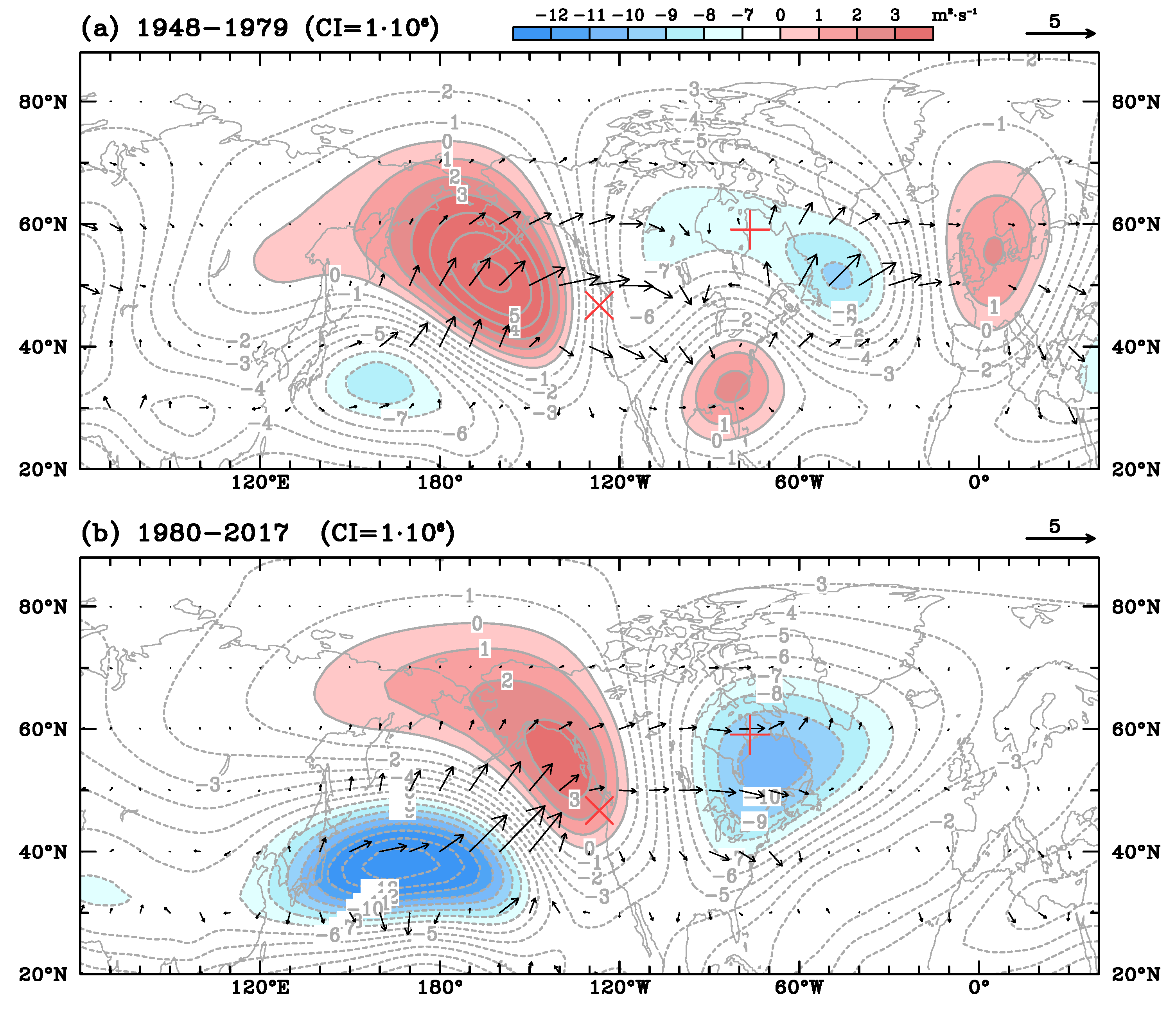
To reveal the associated forcing of teleconnection involved in the circulation pattern change, we conducted the analysis of Rossby Wave Activity Flux (WAF) derived by Takaya and Nakamura (2001) [35] at 250 hPa, regressed upon the PC1 and PC2 time series of Figure 1. A wave-like structure in the upper troposphere (Figure 5) is associated with the wave activity fluxes that suggest two forcing sources: (a) one emanated from the tropical central Pacific during the pre-1980 period; and (b) one from the subtropical western Pacific during the post-1980 period. The downstream WAF over the eastern U.S. regenerate another wave train towards Europe, which is known to the PNA. The upstream WAF after 1980 shifts and expends northward to near Japan. The post-1980 wave train has a more robust cyclonic anomaly in the western Pacific, conveying the energy that enhances the ridge over the Gulf of Alaska while the wave train tracks through northeastern North America. Notably, this wave train is phase-coincident with NAWD (marked by × and + in Figure 5b) and does not re-generate downwind waves towards Europe.

3.2. Past NAWD

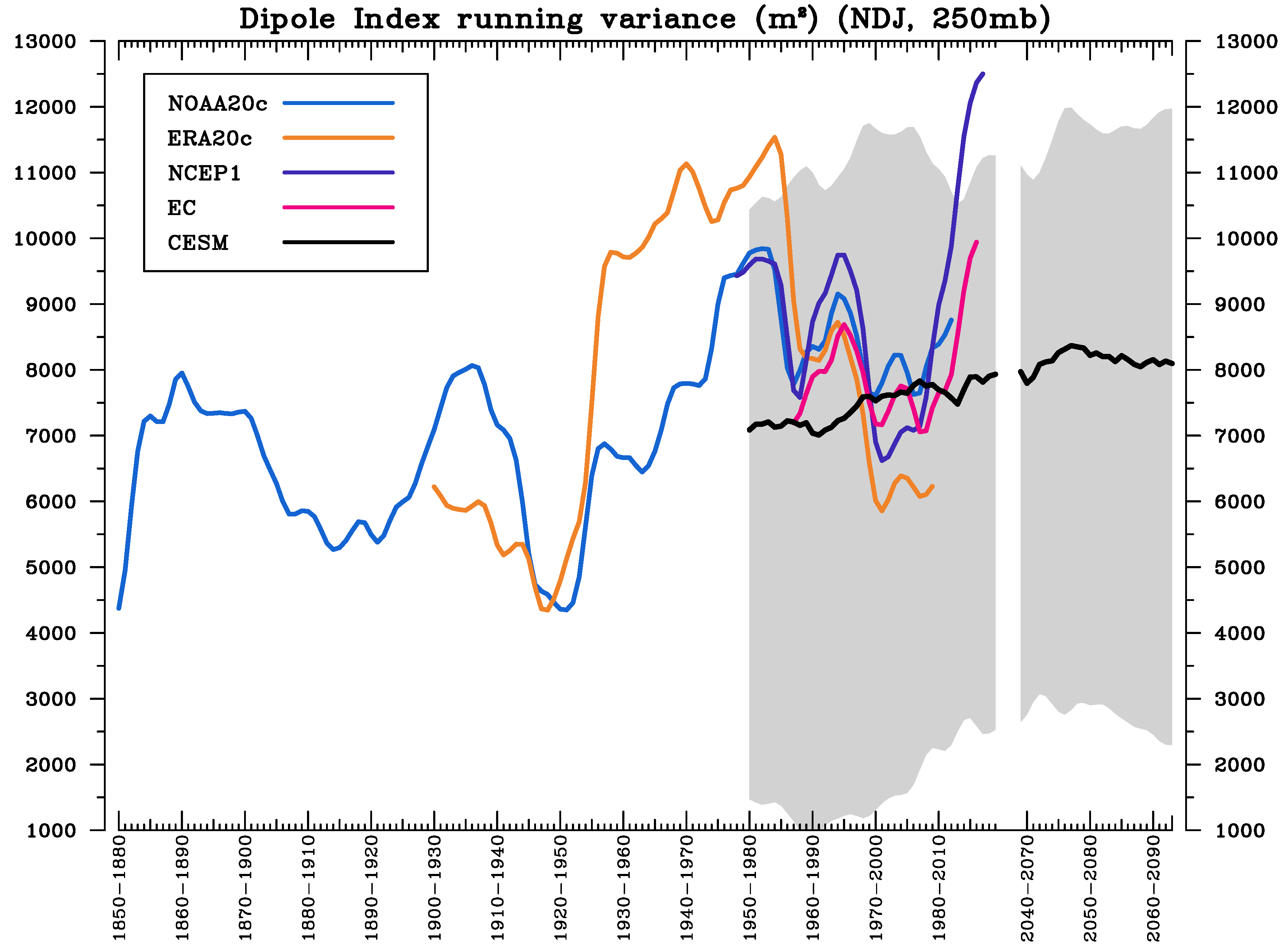
To gain the historical and projected perspectives for the transition between the leading EOF modes of atmospheric circulation, we next computed a 30-year running variance of the NAWD index by following the definition of Wang et al. (2014). Figure 6 shows the running variance of NAWD derived from the NOAA 20CR, the NCEP–NCAR and ERA-Interim reanalysis data, overlaid with the CESM ensemble simulations. NAWD has undergone pronounced inter-decadal variation on the order of 60 years and demonstrated the largest variance in the early 21st century. Similar analyses applied to each CESM ensemble member and averaged as the ensemble mean revealed an increase in the NAWD variance during the historical period (up to 2005 with increasing greenhouse gas), a trend that is projected to continue under the high-emission scenario (RCP 8.5) towards 2080. The projected ensemble-mean variance starts to decline after 2050, despite an increase in the ensemble spread. At this point, we can only attribute this late-21st-century decline of the NAWD variance to the natural variability revealed in the observed period.
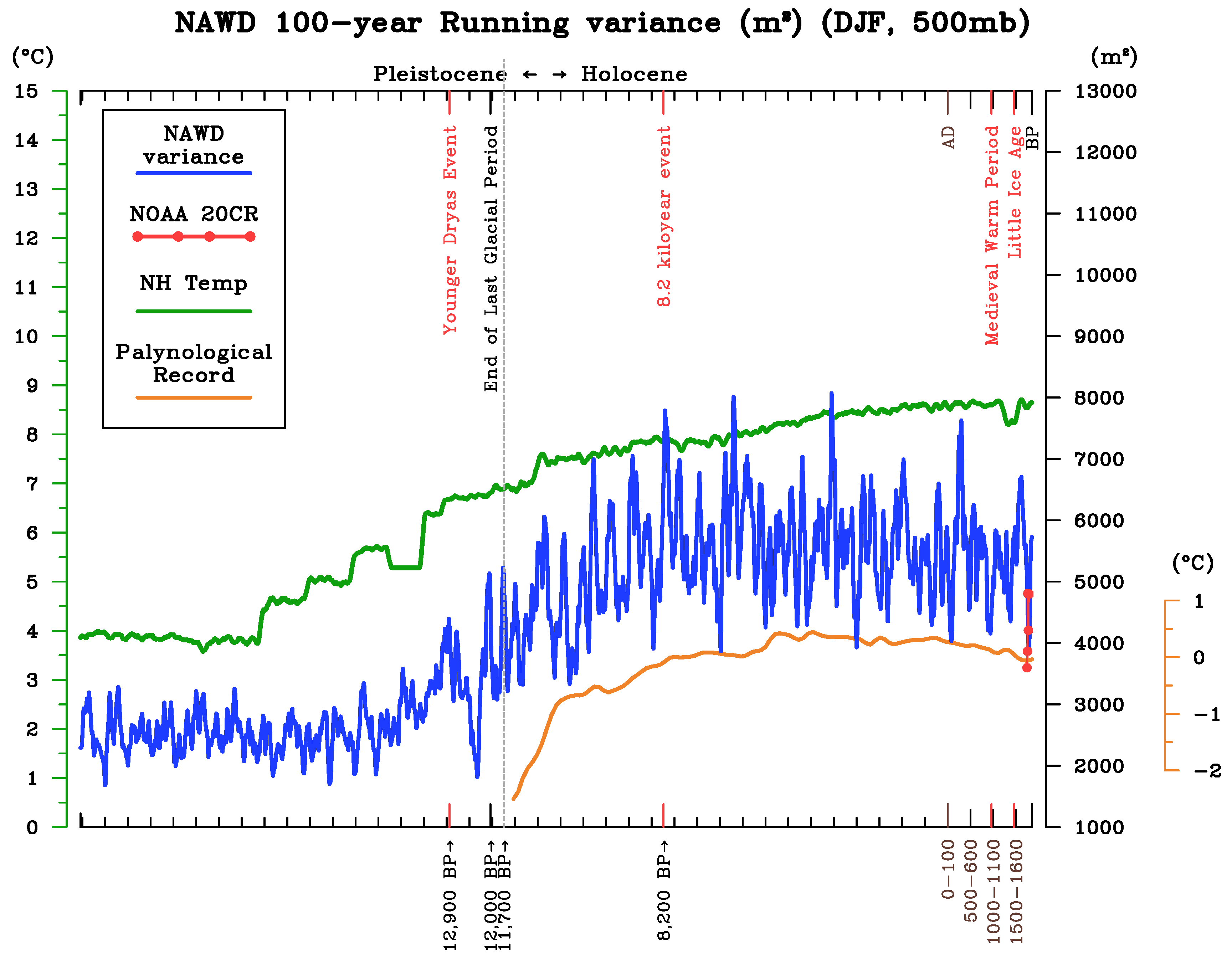
As an alternative means to understand how the NAWD and stationary waves vary with respect to the global temperature change, we applied the same analytical approach to the paleoclimate simulations. Considering the much longer paleoclimate time scale, the running variance was calculated across a 100-year window, with a 10-year interval. Figure 7 displays the reconstructed paleoclimate NAWD index (blue line) and the global and Northern Hemispheric mean surface temperatures (green lines), superimposed with the 20CR’s NAWD 100-year running variance from 1851 to 1950 (red dot in the right end) for comparison. The time series from 20CR and paleoclimate simulations did reveal similar fluctuations during their overlapping years. During the Pleistocene era, the global temperature is lower and NAWD is less variable; during the Holocene with increasing global temperature, the NAWD variance increases significantly and shows a larger fluctuation. The time period after the Younger Dryas event appears to be a turning period in which global temperature and NAWD variability change correspondingly for almost ten centuries. We should note that the paleoclimate dataset has a lower resolution so the NAWD index calculated may not be compatible in magnitude with that of the modern reanalysis data; further, a least-squares regression was applied to approximate the 500-hPa geopotential height to the 250-hPa NAWD index (see Section 2).
During the last glacial period, North America was characterized by a thick layer of ice covering the area that now constitutes the eastern dipole of the NAWD; this would certainly have affected atmospheric circulation patterns beyond that expected from temperature alone. Large ice sheets remained just to the north of the eastern dipole region of central Canada until between 9000 and 7000 years BP and much of the Holocene vegetation types we are familiar with did not occur until 5000 years BP (Williams et al., 2004) [36]. As such, comparisons of NAWD variability to Northern Hemisphere temperature trends over the period from 5000 years BP until the present likely presents the most robust paleo analog for how temperature may affect NAWD into the future. From 5000 years BP to the present, ice core stable isotopes and palynological studies indicate that temperatures across the Northern Hemisphere have slowly declined, and that NAWD variance has also declined (Figure 7). Overall, reconstructions of paleo temperature and simulations support an interpretation of greater energy and temperatures across the Northern hemisphere promoting greater NAWD variability.
We should caution that this paleoclimate model lacks feedback processes in the carbon cycle, vegetation, and terrestrial ice sheets; moreover, ice sheet height of Greenland is different in the past so the circulation–terrain interaction might have impacted the jet stream and subsequent NAWD. It is also possible that the stationary waves’ position experienced some shifting. These aspects require more complete simulations to reveal in future research.

3.3. Possible Forcing Change

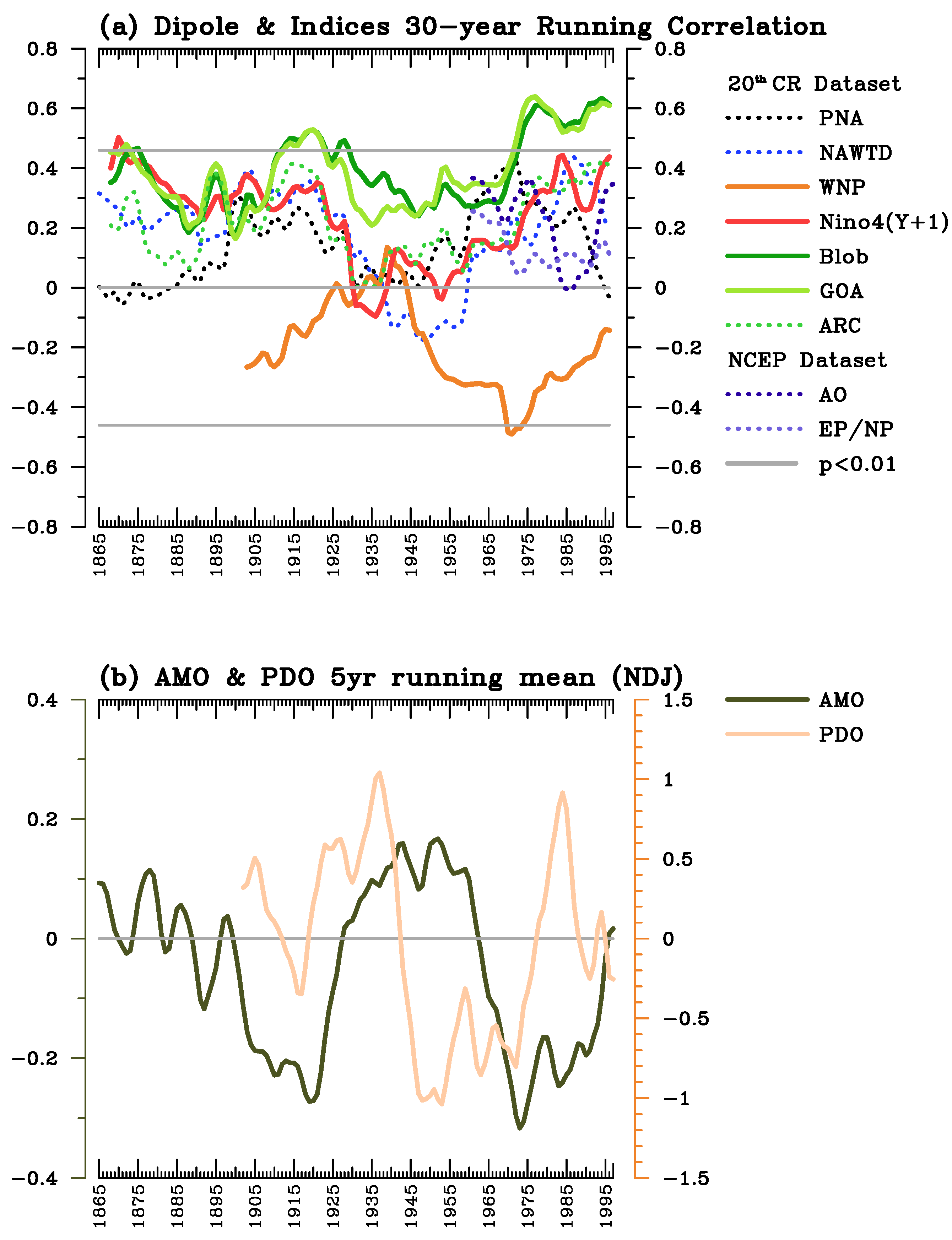
Here, we examine the documented large-scale mode of climate variability linked to the significant 2013–2015 winter anomalies in North America. Figure 8a shows the 30-year running correlation analysis of the NAWD index with the list of relevant climate indices as shown in Table 1 (see Section 2.3). It was found that the Blob, GOA, Niño 4 (Y + 1), and WNP indices are significantly correlated with NAWD (p < 0.05) during the latter 20th century, consistent with the literature. These significant yet episodic correlations imply that NAWD is mostly linked to local SST anomalies in the northeast and northwest Pacific, which is in good agreement with Figure 1d. The increasingly high correlation between the Blob index/GOA index and the Dipole index since 1960 indicates a strengthened relationship of NAWD with SST variations. As mentioned in the last section, the northeast Pacific warm SST patch (or Blob) is induced by an anomalous ridge of high-pressure, which brings cloud-free conditions and excess solar radiation that warms the sea surface.
Lorenzo and Mantua (2016) [23] indicated that the correlation between the EP/NP index and 300 hPa stream function resembles NAWD. However, the correlation between the EP/NP index and NAWD here does not exceed the significance level. As their study suggested, the relationship between EP/NP and the circulation is clearer in the eastern and northern part of the US, but the NAWD index represents the higher-latitude ridge/trough system, which may lead to the insignificant correlation. Lorenzo and Mantua (2016) [23] and Wang et al. (2014) [4] also mentioned that the AO index has a stronger relationship with the southern U.S. This may explain why the correlations of AO and EP/NP with NAWD do not reach statistical significance, but nonetheless show an increasing trend after the mid-1970s. The other indices do not show significant correlations but some do exhibit a growing relationship with the NAWD; this observation infers that constructive interactions between these climate modes could be a compounding mechanism that strengthened NAWD in winter 2013/2014 (Lee et al., 2014) [37].
Here we provide a provisional discussion on the possible role of inter-decadal climate variability in modulating Figure 8a’s low-frequency variations in the sliding correlations: the Atlantic multidecadal oscillation (AMO) and the Pacific decadal oscillation (PDO). It has been suggested that the AMO can impact climate variations in the Pacific Ocean (e.g., Zhang and Delworth 2007) [38]. Figure 8b shows the 5-year running mean of the AMO and PDO indices and, upon visual examination, it appears that the AMO has an inverse, yet corresponding, phasing with the correlations of GOA and the Blob (green lines in Figure 8a). This analysis, though preliminary, suggests a possible role of the natural variability (i.e., the AMO) in modulating the SST-NAWD co-variability in the long run; this feature requires further research.

4. Conclusions

The diagnostics undertaken here suggest that the leading mode of the wintertime atmospheric stationary waves in the Northern Hemisphere has undergone a notable change. Since the 1980s, the first leading mode of anomalous winter stationary eddies in the subseasonal timescale has alternated from the PNA to a comparably strong NAWD. Given that EOF describes the variance of individual patterns, the observed increase in the amplitude of NAWD suggests that it may have overtaken the PNA as the more common type of winter variability, with increased influence from western North Pacific SSTs. The CESM large-ensemble simulations forced with increasing greenhouse gas indicate that the NAWD variance will gradually amplify alongside its low-frequency natural variability. This result implies that the subseasonal variation of the atmospheric circulations over North America could continue to be dominated by the NAWD mode, with the potential to sharpen the east–west temperature and precipitation division across North America.
Further comparison of EOF1/EOF2 with PNA/NAWD using spatial correlation reveals a pattern change that is consistent among different reanalysis datasets. Analysis of the paleoclimate simulations suggests that NAWD does co-vary with the global temperature variation at centennial timescales: the NAWD variance was weak in the cooler Pleistocene and gradually increased and stabilized in the warmer Holocene. We further examined large-scale forcing of both atmospheric and oceanic origins for the amplified NAWD and found that most of the documented climate indices, which showed a connection to the 2013–2014 extreme winter of North America, are insignificantly correlated with NAWD with the exception of certain oceanic features like the WNP and Niño 4 (Y + 1); these imply that regional SST anomalies in the subtropical West Pacific may provoke teleconnections that affect NAWD. Future examination of the dynamic processes leading to the NAWD amplification should consider the stationary waves maintenance, namely the jet–terrain interactions, tropical and extratropical diabatic heating, and the effect of Arctic amplification.

Author Contributions

Y.-T.C. and S.-Y.S.W. designed the research, conducted analyses, and wrote the main part of the manuscript. Y.C., S.L.V., J.D.D.M., and J.-H.Y. contributed to the analysis and writing the paper. All authors discussed the results and reviewed the manuscript.

Funding

This research was supported by the National Science Foundation P2C2 Program award number 1903721, the U.S. Department of Energy, Office of Science, program under award number DE-SC0016605, and the USU Agriculture Experimental Station. J.Y. acknowledges the KMA R&D Program KMI2018-07010 and GIST Research Institute (GRI) grant funded by the GIST in 2019.

Acknowledgments

Y.-T.C. thanks Don. J. Wang for making her study at Utah State University possible.

Conflicts of Interest

The authors declare no conflict of interest.

Abbreviations

The following abbreviations are used in this manuscript:
20CRNOAA Twentieth Century Reanalysis version 2c
AOArctic Oscillation
AGCMAtmospheric General circulation model
B.P.Before Present; 1950A.D.
CESMCommunity Earth System Model
ECMWFEuropean Centre for Medium-Range Weather Forecasts
ERA-20CECMWF global reanalysis products for the twentieth century
EOFEmpirical Orthogonal Function
ENSOEl Nino/Southern Oscillation
LGMLast Glacial Maximum
NHNorth Hemisphere
NOINorthern Oscillation index
PCPrinciple Component
PDOPacific Decadal Oscillation
PNAPacific–North America
SSTSea surface temperature
SSTASea surface temperature anomaly
TNHTropical Northern Hemisphere pattern
WAFWave activity flux
WNPWestern North Pacific pattern
WPWestern Pacific pattern

References

  1. NOAA National Centers for Environmental Information (NCEI). U.S. Billion-Dollar Weather and Climate Disasters. 2019. Available online: https://www.ncdc.noaa.gov/billions/ (accessed on 3 December 2019).
  2. Singh, D.; Swain, D.L.; Mankin, J.S.; Horton, D.E.; Thomas, L.N.; Rajaratnam, B.; Diffenbaugh, N.S. Recent amplification of the North American winter temperature dipole. J. Geophys. Res. Atmos. 2016, 121, 9911–9928. [Google Scholar] [CrossRef] [PubMed] [Green Version]
  3. Wang, S.-Y.S.; Huang, W.-R.; Yoon, J.-H. The North American winter ‘dipole’ and extremes activity: A CMIP5 assessment. Atmos. Sci. Lett. 2015, 16, 338–345. [Google Scholar] [CrossRef] [Green Version]
  4. Wang, S.-Y.S.; Yoon, J.-H.; Becker, E.; Gillies, R. California from drought to deluge. Nat. Clim. Chang. 2017, 7, 465–468. [Google Scholar] [CrossRef]
  5. Stuivenvolt-Allen, J.; Wang, S.-Y.S. Data Mining Climate Variability as an Indicator of U.S. Natural Gas. Front. Big Data 2019, 2, 20. [Google Scholar] [CrossRef] [Green Version]
  6. Voelker, S.L.; Wang, S.-Y.; Dawson, T.E.; Roden, J.S.; Still, C.J.; Longstaffe, F.J.; Ayalon, A. Tree-ring isotopes adjacent to Lake Superior reveal cold winter anomalies for the Great Lakes region of North America. Sci. Rep. 2019, 9, 4412. [Google Scholar] [CrossRef] [PubMed] [Green Version]
  7. Swain, D.L.; Tsiang, M.; Haugen, M.; Singh, D.; Charland, A.; Rajaratnam, B.; Diffenbaugh, N.S. The extraordinary California drought of 2013/2014: Character, context, and the role of climate change [in “Explaining Extremes of 2013 from a Climate Perspective”]. Bull. Am. Meteorol. Soc. 2014, 95, S3–S7. [Google Scholar]
  8. Hartmann, D.L. Pacific sea surface temperature and the winter of 2014. Geophys. Res. Lett. 2015, 42, 1894–1902. [Google Scholar] [CrossRef]
  9. Schulte, J.A.; Lee, S. Strengthening North Pacific influences on United States temperature variability. Sci. Rep. 2017, 7, 124. [Google Scholar] [CrossRef]
  10. Francis, J.A.; Vavrus, S.J. Evidence linking Arctic amplification to extreme weather in mid-latitudes. Geophys. Res Lett. 2012, 22, L068601. [Google Scholar] [CrossRef]
  11. Overland, J.E.; Dethloff, K.; Francis, J.A.; Hall, R.J.; Hanna, E.; Kim, S.; Screen, J.A.; Shepherd, T.G.; Vihma, T. Nonlinear response of mid-latitude weather to the changing Arctic. Nat. Clim. Chang. 2016, 6, 992–999. [Google Scholar] [CrossRef] [Green Version]
  12. Swain, D.L.; Langenbrunner, B.; Neelin, J.D.; Hall, A. Increasing precipitation volatility in twenty-first-century California. Nat. Clim. Chang. 2018, 8, 427. [Google Scholar] [CrossRef]
  13. Yoon, J.H.; Wang, S.S.; Gillies, R.R.; Kravitz, B.; Hipps, L.; Rasch, P.J. Increasing water cycle extremes in California and in relation to ENSO cycle under global warming. Nat. Commun. 2015, 6, 8657. [Google Scholar] [CrossRef] [PubMed] [Green Version]
  14. Wang, S.-Y.; Hipps, L.; Gillies, R.R.; Yoon, J.-H. Probable causes of the abnormal ridge accompanying the 2013–2014 California drought: ENSO precursor and anthropogenic warming footprint. Geophys. Res. Lett. 2014, 41, 3220–3226. [Google Scholar] [CrossRef] [Green Version]
  15. Kalnay, E.; Kanamitsu, M.; Kistler, R.; Collins, W.; Deaven, D.; Gandin, L.; Iredell, M.; Saha, S.; White, G.; Woollen, J. The NCEP/NCAR 40-year reanalysis project. Bull. Am. Meteorol. Soc. 1996, 77, 437–472. [Google Scholar] [CrossRef] [Green Version]
  16. Dee, D.P.; Uppala, S.M.; Simmons, A.J.; Berrisford, P.; Poli, P.; Kobayashi, S.; Andrae, U.; Balmaseda, M.A.; Balsamo, G.; Bauer, P.; et al. The ERA-Interim reanalysis: Configuration and performance of the data assimilation system. Q. J. R. Meteorol. Soc. 2011, 137, 553–597. [Google Scholar] [CrossRef]
  17. Uppala, S.M.; KÅllberg, P.W.; Simmons, A.J.; Andrae, U.; Da Costa Bechtold, V.; Fiorino, M.; Gibson, J.K.; Haseler, J.; Hernandez, A.; Kelly, G.A.; et al. The ERA-40 re-analysis. Q. J. R. Meteorol. Soc. 2005, 131, 2961–3012. [Google Scholar] [CrossRef]
  18. Poli, P.; Hersbach, H.; Dee, D.P. ERA-20C: An atmospheric reanalysis of the twentieth century. J. Clim. 2016, 29, 4083–4097. [Google Scholar] [CrossRef]
  19. Huang, B.; Banzon, V.F.; Freeman, E.; Lawrimore, J.; Liu, W.; Peterson, T.C.; Smith, T.M.; Thorne, P.W.; Woodruff, S.D.; Zhang, H.-M. Extended Reconstructed Sea Surface Temperature version 4 (ERSST.v4): Part I. Upgrades and intercomparisons. J. Clim. 2014, 28, 911–930. [Google Scholar] [CrossRef] [Green Version]
  20. Kay, J.E.; Deser, C.; Phillips, A.; Mai, A.; Hannay, C.; Strand, G.; Arblaster, J.M.; Bates, S.C.; Danabasoglu, G.; Edwards, J.; et al. The Community Earth System Model (CESM) large ensemble project. Bull. Am. Meteorol. Soc. 2015, 96, 1333–1349. [Google Scholar] [CrossRef] [Green Version]
  21. Pegion, K.V.; Selman, C. Extratropical Precursors of the El Niño–Southern Oscillation. In Climate Extremes: Patterns and Mechanisms; Wiley: Hoboken, NJ, USA, 2017; pp. 299–314. [Google Scholar]
  22. Bond, N.A.; Cronin, M.F.; Freeland, H.; Mantua, N. Causes and impacts of the 2014 warm anomaly in the NE Pacific. Geophys. Res. Lett. 2015, 42, 3414–3420. [Google Scholar] [CrossRef]
  23. Lorenzo, E.; Mantua, N. Multi-year persistence of the 2014/2015 North Pacific marine heatwave. Nat. Clim. Chang. 2016, 6, 1042–1047. [Google Scholar] [CrossRef]
  24. Higgins, R.W.; Schemm, J.-K.E.; Shi, W.; Leetmaa, A. Extreme precipitation events in the western United States related to tropical forcing. J. Clim. 2000, 13, 793–820. [Google Scholar] [CrossRef]
  25. Horel, J.D.; Wallace, J.M. Planetary-scale atmospheric phenomena associated with the Southern Oscillation. Mon. Weather Rev. 1981, 109, 813–829. [Google Scholar] [CrossRef]
  26. North, G.R.; Bell, T.L.; Cahalan, R.F. Sampling errors in the estimation of empirical orthogonal functions. Mon. Weather Rev. 1982, 110, 699–706. [Google Scholar] [CrossRef]
  27. Kintisch, E. ‘The Blob’ invades Pacific, flummoxing climate experts. Science 2015, 348, 17–18. [Google Scholar] [CrossRef]
  28. Wang, S.-Y.; L’Heureux, M.; Chia, H.-H. ENSO prediction one year in advance using Western North Pacific sea surface temperatures. Geophys. Res. Lett. 2012, 39. [Google Scholar] [CrossRef] [Green Version]
  29. Wang, S.-Y.; L’Heureux, M.; Yoon, J.-H. Are greenhouse gases changing ENSO precursors in the Western North Pacific? J. Clim. 2013, 26, 6309–6322. [Google Scholar] [CrossRef]
  30. Capotondi, A.; Sardeshmukh, P.D. Optimal precursors of different types of ENSO events. Geophys. Res. Lett. 2015, 42, 9952–9960. [Google Scholar] [CrossRef]
  31. Zhang, X.; Sorteberg, A.; Zhang, J.; Gerdes, R.; Comiso, J.C. Recent radical shifts of the atmospheric circulations and rapid changes in the Arctic climate system. Geophys. Res. Lett. 2008, 35, L22701. [Google Scholar] [CrossRef] [Green Version]
  32. Zhou, Z.-Q.; Xie, S.-P.; Zheng, X.-T.; Liu, Q.; Wang, H. Global warming-induced changes in El Niño teleconnections over the North Pacific and North America. J. Clim. 2014, 27, 9050–9064. [Google Scholar] [CrossRef] [Green Version]
  33. Johnson, N.C.; Feldstein, S.B. The continuum of North Pacific sea level pressure patterns: Intraseasonal, interannual, and interdecadal variability. J. Clim. 2010, 23, 851–867. [Google Scholar] [CrossRef]
  34. Chang, E.K.M. Diabatic and orographic forcing of northern winter stationary waves and storm tracks. J Clim. 2009, 22, 670–688. [Google Scholar] [CrossRef]
  35. Takaya, K.; Nakamura, H. A formulation of a phase-independent wave-activity flux for stationary and migratory quasi-geostrophic eddies on a zonally varying basic flow. J. Atmos. Sci. 2001, 58, 608–627. [Google Scholar] [CrossRef]
  36. Williams, J.W.; Shuman, B.N.; Webb, T.; Bartlein, P.J.; Leduc, P.L. Late-quaternary vegetation dynamics in north america: Scaling from taxa to biomes. Ecol. Monogr. 2004, 74, 309–334. [Google Scholar] [CrossRef] [Green Version]
  37. Lee, M.-Y.; Hong, C.-C.; Hsu, H.-H. Compounding effects of warm sea surface temperature and reduced sea ice on the extreme circulation over the extratropical North Pacific and North America during the 2013–2014 boreal winter. Geophys. Res. Lett. 2015, 42, 1612–1618. [Google Scholar] [CrossRef]
  38. Zhang, R.; Delworth, T.L. Impact of the Atlantic multidecadal oscillation on North Pacific climate variability. Geophys. Res. Lett. 2007, 34, L23708. [Google Scholar] [CrossRef] [Green Version]
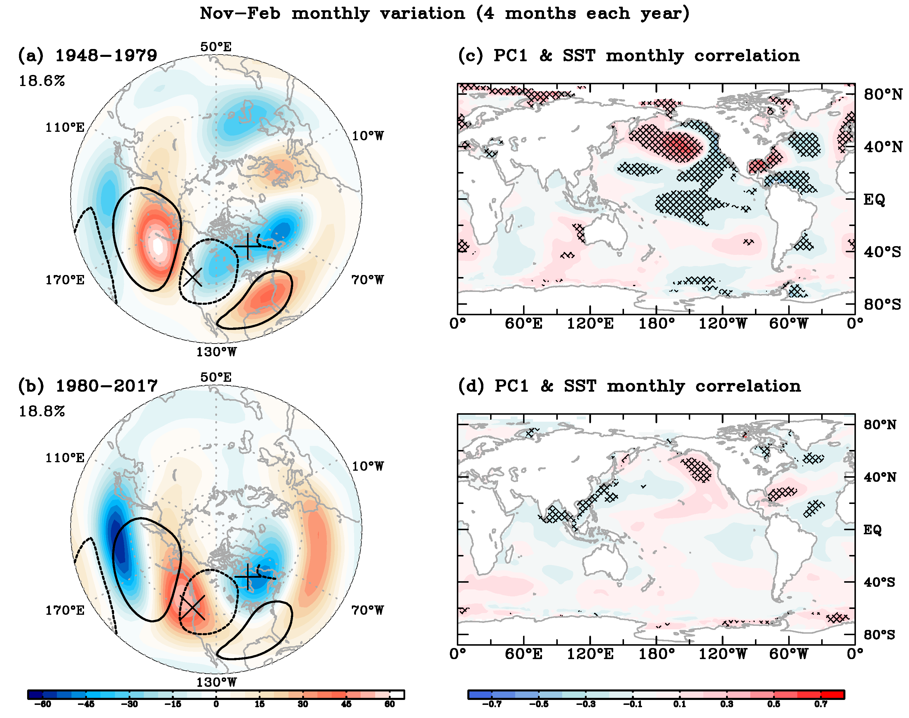
Figure 1. Empirical orthogonal function (EOF) analysis results of (a) 1948–1979 and (b) 1980–2017 with the PNA pattern superimposed and the dipole centers marked with × and + in North America. The correlation map between monthly SST anomalies and the first principle component (PC1) for (c) 1948–1979 and (d) 1980–2017.
Atmosphere 10 00793 g001
Figure 2. Percent of variance explained for Δ Z E 250 during (a) 1948–1979 and (b) 1980–2017. Only the first four modes are presented.
Atmosphere 10 00793 g002
Figure 3. First and second EOF modes of NDJF winter seasonal mean Δ Z E 250 for the early period (1948–1979) (a,c) and the late period (1980–2017) (b,d). The Dipole centers (marked with × and +) are superimposed with the PNA pattern (contour) as in Figure 1. The percent of variance each EOF mode explains is listed as well.
Atmosphere 10 00793 g003
Figure 4. Spatial correlation coefficients between PNA/Dipole pattern and (a) EOF1 (b) EOF2 results. EOF analysis and the spatial correlations are conducted via a five-year sliding-EOF window with three different datasets.
Atmosphere 10 00793 g004
Figure 5. The regressed NDJF monthly 250-hPa Streamfunction (Gray lines for contour; interval (CI) = 1 × 10⁶) during (a) 1948–1979 and (b) 1980–2017. Vectors represent the associated horizontal component of the wave activity flux (m2 s−2).
Atmosphere 10 00793 g005
Figure 6. The 30-year running variance of the Dipole index (DPI) derived from Wang et al. (2014) by using multiplied reanalysis datasets. Gray shaded represents CESM 40-member ensemble spread, which represents two standard deviations from the ensemble mean.
Atmosphere 10 00793 g006
Figure 7. The 100-year running variance of the NAWD index (DJF mean, 500 hPa; blue line) derived using paleoclimate and 20CR dataset. The green line represents the Northern Hemisphere temperature mean, with notable historical listed. The orange line represents continental reconstruction temperature derived from palynological record, with anomalies relative to the 1450–1950 A.D. mean.
Atmosphere 10 00793 g007
Figure 8. The x-axis presents the middle era for: (a) The 30-year running correlation of the Dipole index and Climate indices. The solid lines represent that the index exceeds the significant level; the dotted lines show the index does not exceed the significant level. Gray lines indicate significant value (p < 0.01). (b) The five-year running average for AMO and PDO index.
Atmosphere 10 00793 g008
Table 1. Climate indices which can be linked to the North America winter anomaly events. A brief description of the index and the corresponding reference is presented.
IndexBrief DescriptionReference
PNAPacific/North American Pattern:Leathers, David. J. (1991)
The variation of atmospheric circulation patterns over the Pacific Ocean and North America.
NAWTDNorth American Winter Temperature Dipole:Singh et al. (2016)
A similar warm-west and cool-east surface temperature dipole pattern in North America
WNPWestern North Pacific:Wang et al., 2013
Connecting the major ENSO precursors
EP/NPEast Pacific/North Pacific:Schulte and Lee (2017)
The positive phase is associated with an amplified jet stream configuration in which a ridge is situated over Alaska and a trough is situated over the eastern US.Schulte and Georgas (2017)
AOArctic Oscillation:Schulte and Lee (2017)
When the AO is in its positive phase, a ring of strong winds circulating around the North Pole acts to confine colder air across polar regions.
AMOAtlantic Multidecadal Oscillation:Zhang and Delworth (2007)
A long-duration changes in the sea surface temperature of the North Atlantic Ocean, with cool and warm phases that may last for 20–40 years.
PDOPacific decadal Oscillation:Mantua, Nathan. J. (1997)
Leading PC of monthly SST anomalies in the North Pacific Ocean
Nino 4East Central Tropical Pacific SSTCPC
(Y + 1)(5 N–5 S; 170–120 W)
BlobPacific blob region: (40–50 N, 150–135 W)Kintisch (2015)
The remarkably warm water mass in the northeastern (NE) Pacific that persisted during 2013–2015
GOAGulf of Alaska index:Lorenzo and Mantua (2016)
This index directed from (1) SSTa and (2) SLPa. The region defined by the 2014/2015 SST peak anomalies near the Gulf of Alaska.
ARCARC pattern:Lorenzo and Mantua (2016)
This index is directed from (1) SSTa and (2) SLPa. Identified by the largest warm anomalies along the entire Pacific North American coastal boundary.