Implicit Definition of Flow Patterns in Street Canyons—Recirculation Zone—Using Exploratory Quantitative and Qualitative Methods

Abstract

Air pollution is a major health hazard for the population that increasingly lives in cities. Street-scale Air Quality Models (AQMs) are a cheap and efficient way to study air pollution and possibly provide solutions. Having to include all the complex phenomena of wind flow between buildings, AQMs employ several parameterisations, one of which is the recirculation zone. Goal of this study is to derive an implicit or explicit definition for the recirculation zone from the flow in street canyons using computational fluid dynamics (CFD). Therefore, a CFD-Large Eddy Simulation model was employed to investigate street canyons with height to width ratio from 1 to 0.20 under perpendicular wind direction. The developed dataset was analyzed with traditional methods (vortex visualization criteria and pollutant dispersion fields), as well as clustering methods (machine learning). Combining the above analyses, it was possible to extract qualitative features that agree well with literature but most importantly to develop quantitative expressions that describe their topology. The extracted features’ topology depends strongly on the street canyon dimensions and not surprisingly is independent of the wind velocity. The developed expressions describe areas with common flow characteristics inside the canyon and thus they can be characterised as an implicit definition for the recirculation zone. Furthermore, the presented methodology can be further applied to cover more parameters such us oblique wind direction and heated-facades and more methods for data analysis.

1. Introduction

Poor air quality is the cause of many health issues, ranging from problems in the cardiovascular and respiratory system [1,2], to food-related allergies [3] and even lung cancers [4]. Its impact on the quality of life [5,6] is indicated by the seven millions deaths in 2012, corresponding to one out of eight deaths globally [7]. Focusing on city streets, the most direct contribution originates from traffic [8] and other sources, such as the wood and oil consumption for heating [9], the industry [10] and natural sources [11]. Naturally, air pollution becomes an important concern for the people who exercise urban planning and design [12,13,14].

Air quality can be assessed by experimental and numerical methods, such as wind tunnel experiments [15], field measurements [16,17,18], Computational Fluid Dynamics (CFD) models [19,20,21,22] and Air Quality Models (AQMs) [23]. From those methods, the AQMs require less personnel training and computational power, compared to experiments and CFD [24], but most importantly they need minimum weather data. Thus, they can be a fast and economic tool of study for urban planners [25,26,27]. Herein, emphasis is on AQM and a specific challenge that will be discussed later, therefore, interested readers are advised to review information on AQM in any of the aforementioned studies.

Regarding their efficiency, street-scale AQMs depend on empirical and semi-empirical parametrisations and assumptions. One of them is the consideration for the recirculating vortices that dominate the lower part of the atmosphere between buildings. These flow structures have been observed in all the relevant experimental and numerical studies and have been found to restrict the removal of pollutants to the upper atmosphere [15,28,29,30,31,32]. Moreover, the partial recirculation of pollutants from the downwind to the upwind side results in different concentrations for each side of the same street [33], with implications on regulatory monitoring and personal exposure assessment.

Street-scale AQMs have parameterised the recirculation either implicitly or explicitly [23,24]. For instance, the STREET-SRI model [34,35] defined a single vortex covering the whole canyon. Two concentrations were calculated for the upwind and downwind sides of the canyon, by employing empirical formulas. The recirculation was considered implicitly by the parameters of those formulas, as they were calculated from field experiments data in cities (i.e., San Jose, CA, USA). Later, the Canyon Plume Box Model [36] regarded three regions inside the canyon, each with a distinct transport mechanism: (i) the entrainment of relatively clean air in the downwind side, (ii) the removal of pollutants by the advective flow in the upwind side, and (iii) the slow pollutant removal from the middle of the canyon due to a weak diffusive flux. An explicit box model (mass balance) accounted for the recirculation, the empirical incoming and outcoming fluxes of which came from field observations in Cologne, Germany.

The STREET-SRI and CPBM were developed based on street canyons with an aspect ratio of building height to the street width (or AR), close to the unity. For this case a large vortex dominates the whole flow, with usually three smaller co-existing vortices, e.g., [37,38,39]. To expand the use of AQMs to wider canyons, the Operational Street Pollution Model (OSPM) [40] introduced the recirculation zone. This was defined as a trapezoid box model, whose dimensions were connected to the street canyon geometry. The ventilation of the box model was assumed to occur through the perimeter of the trapezium, namely the top and the lateral edges. Thus, for wide street canyons (AR < 0.5), the pollutants were dispersed through those edges. On the other hand, for narrow street canyons (AR > 0.5) the lateral edge was further blocked by the downwind building and the pollutants were dispersed only through the top [33]. The expression of the recirculation as a function of the AR was also employed in models, such as AEOLIUS [41], ADMS [42] and others [43,44,45].

Finally, a different approach was adopted by SIRANE [46,47], which assumed that recirculation creates a well-mixed region with a uniform pollutant concentration for the whole street canyon. For SIRANE, narrow roads with AR larger than 1/3 were assumed to be affected by recirculation and thus treated as street canyons, while wider roads were treated as open terrain.

The current study elaborates on the hypothesis that the recirculation zone is correlated with the flow characteristics and consequently with the boundary conditions of the problem. Therefore, the former recirculation zone could be implicitly and directly approximated from the boundary conditions without the need to conduct intensive numerical calculations (e.g., CFD). Of course, this is not a new hypothesis and as described earlier street-scale AQMs employed several approaches to model the effect of recirculation. However, aim of this study is to devise a universal description but implicit correlation that could eliminate the need of empirical and human interventions (e.g., the 1/3 AR in SIRANE). Such a description should be (i) based on the systematic analysis of the flow characteristics, (ii) verified in simple geometries, and (iii) expanded for more complex geometries and in parallel extending the applicability of AQMs.

To achieve this, Large Eddy Simulations (LES) were developed and compiled into a hefty dataset of high temporal and spatial resolution flow and dispersion characteristics of street canyon pollution scenarios (Section 2.1); in the absence of equivalent field measurements. This large dataset was processed and analysed using two quite different approaches: vortex visualization (Section 2.2), and k-means cluster analysis (Section 2.3). The first one has been suggested or utilised in the past for similar objectives. The latter refers to a technique of the large family of unsupervised learning methods that are employed in exploratory data analysis. Other methods were also tested but did not contribute to this work, some are mentioned in the related paragraphs. Initially, the outcomes from each approach are presented as calculated (Section 3) and later they are combined and discussed towards the aforementioned hypothesis (Section 4).

2. Methodology

In this chapter, as it was mentioned earlier, the main components of the employed methods are presented. We exhibit the selected simulation set-up and proceed with the three employed methods to analyse the velocity field.

2.1. Simulation Set-up

The wind flow inside street canyons will be studied, to examine different ways that the recirculation zone can be systematically described for a range of aspect ratios H/W (hereafter AR). Hence the focus is on the area between the two buildings and as a result the quasi-2D set-up will be employed. This LES set-up effectively studies the case of perpendicular wind direction as the simplest boundary condition and the most burdening scenario for the air quality [47]. The employed set-up in this paper, has been extensively utilised in similar projects, e.g., [48,49,50]. The physical geometry and boundary conditions are summarised in Figure 1a, while the x-z cross-section of the discretised domain is shown in Figure 1b.

An LES methodology [51,52] was selected for resolving the unsteady, three-dimensional incompressible filtered Navier–Stokes equations for continuity and momentum [53], which can be written in Cartesian tensor notation as follows:

Filtered continuity equations:

$$\frac{\partial {\overline{u}}_i}{\partial x_i}=0$$

(1)

Filtered momentum equations:

$$\frac{\partial {\overline{u}}_i}{\partial t}+\frac{\partial {\overline{u}}_i{\overline{u}}_j}{\partial x_j}=-\frac{1}{\rho }\frac{\partial \overline{p}}{\partial x_i}-\frac{\partial {\tau }_{ij}}{\partial x_j}+v\frac{{\partial }^2{\overline{u}}_i}{\partial x_j\partial x_j}$$

(2)

where ${\overline{u}}_i$ is the filtered mean velocity component in the i-direction, ${\overline{u}}_j$ is the filtered mean velocity component in the j-direction, x_i,j is the distance in the i-and j-directions, $\overline{p}$ is the filtered pressure, v is the kinematic molecular viscosity, ρ is the density, t is the time and the subscript indices i, j (= 1, 2, 3) denote the three space coordinates and ${\tau }_{ij}$ is the subgrid-scale (SGS) stress tensor.

The SGS stress tensor represents the sub-grid part of turbulence and is modelled with the Boussinesq approximation:

$$\underset{\mathrm{deviatoric}}{\underbrace{{\tau }_{ij}-\frac{1}{3}{\tau }_{kk}{\delta }_{ij}}}+\underset{\mathrm{isotropic}}{\underbrace{\frac{1}{3}{\tau }_{kk}{\delta }_{ij}}}=-2v_{\mathrm{sgs}}{\overline{S}}_{ij}$$

(3)

where the isotropic part is embedded in the modified filtered static pressure term, while the deviatoric part is assumed to be proportional to the resolved strain rate tensor ${\overline{S}}_{ij}$, through the eddy viscosity, v_sgs.

The resolved strain rate tensor ${\overline{S}}_{ij}$ is written as:

$${\overline{S}}_{ij}=\frac{1}{2}\left(\frac{\partial {\overline{u}}_i}{\partial x_j}+\frac{\partial {\overline{u}}_j}{\partial x_i}\right)$$

(4)

The eddy viscosity v_sgs is modelled with the k-equation model by Yoshizawa and Horiuti [54], by resolving the transport equation of SGS kinetic energy, $k_{\mathrm{sgs}}=\frac{1}{2}\left(\overline{u_k{u}_k}-{\overline{u}}_k{\overline{u}}_k\right)$:

$$\frac{\partial k_{\mathrm{sgs}}}{\partial t}+\frac{\partial k_{\mathrm{sgs}}{\overline{u}}_j}{\partial x_j}=\frac{\partial }{\partial x_j}\left[\left(v+v_{\mathrm{sgs}}\right)\frac{\partial k_{\mathrm{sgs}}}{\partial x_j}\right]-{\tau }_{ij}{\overline{S}}_{ij}-C_{\mathrm{e}}\frac{k_{\mathrm{sgs}}^{3/2}}{\Delta }$$

(5)

and the eddy viscosity is given as:

$$v_{\mathrm{sgs}}=C_{\mathrm{k}}{k}_{\mathrm{sgs}}^{1/2}\Delta$$

(6)

where C_k (=0.094) and C_e (=1.048) are the model constants and Δ is the filter width, associated with the cell dimensions Δ_i, Δ = (Δ_xΔ_yΔ_z)^1/3. The terms in the right hand of Equation (5) represent the diffusion, production and dissipation of k_sgs, respectively. The constants C_k and C_e are calculated with the assumption of balance between SGS energy production and dissipation rates [55]. The transport equation implies that the historic effects of production, dissipation, and diffusion of the k_sgs are captured.

Finally, the dispersion of the pollutant is resolved with a convection–diffusion equation:

$$\frac{\partial \overline{C}}{\partial t}+\frac{\partial \left({\overline{u}}_i\overline{C}\right)}{\partial x_i}=\frac{\partial }{\partial x_i}\left(D_{\mathrm{total}}\frac{\partial \overline{C}}{\partial x_i}\right)+P$$

(7)

where $\overline{C}$ is the pollutant’s concentration, P are the characteristics of the pollutant source (i.e., geometry and emission rate) and D_total is the total diffusion coefficient:

$$D_{\mathrm{total}}=D+\frac{v_{\mathrm{sgs}}}{S{c}_{\mathrm{t}}}$$

(8)

where D is the molecular diffusion coefficient and Sc_t is the turbulent Schmidt number. The value of Sc_t is taken equal to 0.7, in accordance with previous atmospheric dispersion studies [56,57], while D is equal to 1.64⋅10⁻⁵ m²⋅s⁻¹, which is the molecular diffusion coefficient for CO₂ at 25 °C [58], as a typical pollutant.

For the implementation of this set-up, the coupling of pressure and velocity is solved by the Pressure-Implicit with Splitting of Operators (PISO) algorithm [59]. The solver is provided by OpenFOAM 5.0 [60] as pisoFoam and is modified to resolve the convection–diffusion equation for a passive scalar, at every time-step. A scalar pollutant source in the middle of the canyon was implemented for each studied case, with the topoSet utility of OpenFOAM. The pressure equation is treated implicitly by the PCG solver using the DIC preconditioner, while the momentum equations are resolved by a simple solver, namely smoothsolver in OpenFOAM, along with the GaussSeidel smoother. All the terms of the equations were discretised with second-order numerical schemes as suggested [61]. The time first derivative is discretised with the backward difference scheme (backward in OpenFOAM), while the UMIST scheme [62] is employed for the convective terms. The gradient and the Laplacian terms are discretised using the central difference schemes, Gauss linear and Gauss linear corrected [60], respectively.

At the top of the domain, the symmetry boundary condition (symmetryPlane in OpenFOAM) was set, following the common practice for the quasi-2D set-up, e.g., [37,56,63]. This means that the normal velocity on this patch is assigned to zero and for the scalars there is a zero-normal gradient.

Periodic (cyclic in OpenFOAM) conditions are used for the streamwise and the spanwise directions, again as the common practice for the quasi-2D configuration. The recycling of the random small velocity vectors for the spanwise direction is not affecting the main flow. The desired streamwise velocity is achieved by using the patchMeanVelocityForce (in system/fvOptions) utility that provides the necessary driving force in the form of a pressure gradient. The recycling of pollutants in the streamwise direction is countered, by overwriting C at the inlet patch, at every time-step with the utility scalarFixedValueConstraint. As the simulation of the wind flow evolves with time, gradually the turbulence inside the street canyon dissipates forming the expected recirculating vortex, while the turbulence in the upper atmosphere creates a realistic wind profile.

The wall boundaries were set to no-slip condition for the velocity field (fixedValue in OpenFOAM):

$${\overline{u}}_i=0;{\overline{u}}_j=0;{\overline{u}}_k=0$$

(9)

The fixed gradient (zeroGradient in OpenFOAM) was used for the scalar parameters:

$$\frac{\partial \phi }{\partial x_i}=0;\frac{\partial \phi }{\partial x_j}=0;\frac{\partial \phi }{\partial x_k}=0$$

(10)

where φ is the scalar quantity, i.e., p, v_sgs, and C.

For the treatment of the flow near the walls, we applied the logarithmic wall function nutkWallFunction as implemented in OpenFOAM:

$$v_{\mathrm{sgs}}=v\left(\frac{\mathsf{\kappa }{y}^{+}}{\ln \left(\mathrm{E}{y}^{+}\right)}-1\right)$$

(11)

where κ = 0.41 is the von Karman’s constant and E = 9.8 is a constant that describes the velocity profile near the wall. y⁺ is the dimensionless wall distance, being defined as u*·y/v, u* is the friction velocity and y is the distance from the wall. The v_sgs is estimated using Equation (12) for values of y⁺ > 11, or else it is assumed that v_sgs = 0.

The domain was discretised with a fully structured and hexahedral grid, with 120 cells per building height. For instance, in the case of building height to street width AR = 0.5, W is discretised by 240 cells, while the height and width of the buildings are constantly discretised with 120 and 60 cells, respectively. This depth of the street canyon satisfies the demand for three-dimensional LES [61]. The employed grids for AR = 1, 0.50, 0.33, 0.25 and 0.20 are 2,592,000, 4,320,000, 6,048,000, 7,776,000 and 9,504,000 cells, respectively.

The 19 studied combinations of AR and reference velocity are compiled into a comprehensive dataset. The scenarios are presented in

Table 1. The reference velocity (U_ref), aspect ratio (AR = H/W) and encoding for the studied cases.

Uref	AR	Code
1.5	0.25	U1.5AR025
1.5	0.33	U1.5AR033
1.5	0.50	U1.5AR050
1.5	0.67	U1.5AR067
1.5	1.00	U1.5AR100
3	0.25	U3AR025
3	0.33	U3AR033
3	0.50	U3AR050
3	1.00	U3AR100
5	0.20	U5AR020
5	0.25	U5AR025
5	0.33	U5AR033
5	0.50	U5AR050
5	0.67	U5AR067
5	1.00	U5AR100
7	0.25	U7AR025
7	0.33	U7AR033
7	0.50	U7AR050
7	1.00	U7AR100

and for the rest of the paper, these cases are encoded using both numbers, e.g., U7AR025 for U_ref = 7 m·s⁻¹ and AR = 0.25, U1.5AR100 for U_ref = 1.5 m·s⁻¹ and AR = 1, etc.

The workflow to arrive to this LES set-up was presented and discussed in our previous paper [64]. In this paper, comparisons are presented for the unity street canyon U5AR100 for the middle of the canyon with x/W = 0.50. The average horizontal (U_mean/U_ref) and vertical velocities (W_mean/U_ref), and their standard deviations (σ_U/U_ref and σ_W/U_ref) are presented in Figure 2. For comparison, there are also presented experimental data from Brown, et al. [65] at Re = 30,000, Li, et al. [66] at Re = 12,000 and from Chew, et al. [67] at Re = 62,000. Furthermore, the LES data with 96 cells per building height are presented from Li, Liu and Leung [49], to have a comparison with another LES. Finally, the wind tunnel experiment at Re = 67,000 and the LES with a discretisation of 400 cells per building height and street width, are presented from Kikumoto and Ooka [68].

The comparison between U5AR100 and the numerical and experimental data is excellent for the horizontal velocity U_mean/U_ref for LES and experimental data, as shown in Figure 2a. The comparison for the vertical velocity W_mean/U_ref in Figure 2b has some discrepancies. It is excellent in agreement with the LES data by Li, Liu and Leung [49]. On the other hand, it is problematic for the comparison with the three available experimental data sets. This was also pointed in our previous work [64] and occurs for x/W = 0.50, while the comparisons are excellent for x/W = 0.25 and 0.75 (not presented here). Nevertheless, all the tested SGS models and even the denser mesh (180 cells per height, instead of 120) did not solve the problem, but all the other validation metrics (i.e., LES_IQ_v, FAC2, NMSE) were within the acceptable limits [64,69,70].

The comparison for the standard deviation of the horizontal velocity σ_U/U_ref in Figure 2c is also excellent between U5AR100 and the experimental work from [66] for the whole range of z/H, while is good for the height of the building with the high resolution LES by Kikumoto and Ooka [68]. It should be considered that their grid resolution is far greater than ours (400 instead of 120) and still the results are comparable in accuracy. Finally, the standard deviation of the vertical velocity σ_W/U_ref is in good agreement with the numerical and experimental data in Figure 2d. From these comparisons and previous [64], the agreement between the current LES and the experimental and numerical data is judged as satisfactory.

2.2. Vortex Visualisation

The goal of this study is to find common characteristics for the flow, between canyons with different AR and connect them in a systematic description for the recirculation zone. Thus, the first approach will be the visual comparison of the flow fields. To make flow structures more obvious and objective, standard visualisation tools are applied. Streamlines are the most common, they represent the path of passively transported particles, and highlight the shape of vortices, but do not always define the vortex with clarity. Thus, further vortex identification criteria will be employed, to indicate the existence of stable vortices [71,72].

Vorticity is the curl of velocity $\overrightarrow{\omega }=\nabla \times \overrightarrow{u}$ and aims to visualise the local spinning motion of the flow. More advanced criteria, such as Q and λ₂, analyse the local gradient velocity tensor, defined as $\nabla \overrightarrow{u}$ = S² + Ω², where S and Ω are the rate-of-strain (symmetric) and vorticity (asymmetric) tensors, respectively. For example, the λ₂ criterion [73] assumes the vortex centre to exist in regions of minimum pressure, when the effects of unsteady straining and viscosity are removed. It is assumed to occur when the second largest eigenvalue (namely λ₂) of S² + Ω² is negative. Similarly, according to the Q criterion [74], a vortex exists where the vorticity magnitude is larger than the strain rate magnitude [75]. This occurs for positive values of the second invariant of $\nabla \overrightarrow{u}$, i.e., $Q=\frac{1}{2}\left({\left|\right|\mathbf{\Omega }\left|\right|}^2-{\left|\right|\mathbf{S}\left|\right|}^2\right)>0$. These methods have been implemented for the identification of vortices into atmospheric flows for both low [76] and high Re numbers [77,78,79].

2.3. K-means Clustering

The results of vortex visualisation criteria revealed that all of them required some user-intervention to classify the flow regions into usable sets. However, this requirement is against our goal to derive a user-free classification of the flow characteristics. Since, our goal is the literal division of the street canyon geometry into regions with “similar” flow characteristics, the application of clustering methodologies was a reasonable next step.

Clustering techniques are a widespread tool in data analysis and have been recently utilised in fluid dynamics [80]. Some applications were also recorded in the general study of air quality problems. The k-nearest method was used to classify the level of air pollution as high, medium and low in 18 monitoring stations in Shanghai [81]. The selected parameters for clustering were the average daily and hourly concentrations of 8 pollutants and a series of urban form characteristics. Similarly, the k-means method was used to classify road traffic, according to travel speed, composition of vehicle fleet and fuel type [82]. Finally, the size of airborne particles was divided in groups in order to extract their characteristic sizes and to simplify the further study [83].

Multiple clustering methodologies were tested, employing the most import flow properties that exist in the quasi-2D geometry, i.e., the average horizontal and vertical velocities U and W and the concentration C. The employed methods were the k-means [84], DBSCAN [85], Ward [86], Birch [87] and Mean Shift [88]. For the implementation of all the examined methods, we used the scikit-learn Python library [89], while the data was processed using Python v3.6.

Among them, the k-means clustering method presented the most consistent results, i.e., continuous regions that appeared systematically for the studied street widths. For this method to work, the user needs to assign a specific number of clusters, in which the observations will be divided, e.g., four for our case. The method begins by randomly characterising the same number of group centres (i.e., four) and calculates the average distance of each centre to its neighbouring observations. The average distance of the observations to the centre is calculated. Then, the method iteratively reassigns centres to other observations, so that the average relative distance of each cluster’s data observations, to the selected cluster centre is minimised [90].

3. Results

3.1. Vortex Visualisation

In this section, we present the visualisations of the velocity flow, the pollutant dispersion field and the vortex visualization criterion λ₂. Figure 3 depicts the flow and dispersion statistics for the cases U5AR100, U5AR033 and U5AR020. More specifically, it is observed that in U5AR100 (Figure 3a) a single vortex dominates the whole street, which occurs also for AR = 0.67 (see Figure S1 of supplementary material), indicating the skimming flow regime. For wider canyons, e.g., U5AR033 and U5AR020 in Figure 3b,c the pattern consists of a large vortex attached in front of the downwind building and one or more weaker vortices behind the upwind one, indicating the wake interference flow regime.

The λ₂ and Q criteria resulted to almost the same outcome, so only the first is presented. The λ₂ is plotted for the three ARs in Figure 3d–f, for the values in the range of 0–0.001. Thus, the larger vortices are highlighted and the smaller rotational flows (but not complete vortices) are bypassed. For the cases U5AR100 and U5AR033, the areas highlighted by λ₂ correspond to the vortices shown by the streamlines Figure 3a,b. This does not occur for U5AR020, as only the part of the highly rotational flow in front of the downwind building has been identified (Figure 3c). This is indicative of a stretched and less rotational vortex, as the canyon becomes wider and the flow regime begins transitioning to isolated roughness.

In Figure 3g, the concentration C_mean/C_max is larger for U5AR100 as expected, which can be attributed to the skimming flow regime, with the higher concentrations appearing at the upwind side. On the other hand, for U5AR033 and U5AR020 Figure 3h,i, the concentration is lower, indicating a better street ventilation. The higher concentration values are located near the source, in the middle of the canyon and close to the ground, because of the weaker flow at this point. For all the cases, the field of dispersion for the scalar pollutant covered the area of the canyon from the location of the source (in the middle) up to the upwind building. Finally, for the vertical velocity W_mean/U_ref Figure 3j,k, the larger positive values are observed in front of the upwind building for U5AR100 and in the middle of the canyon for U5AR033 and U5AR020. This is the location where the main vortex ends for all cases. The results of the methods described in Section 2.1, provided some basic and qualitative information about the characteristics of the flow and dispersion for the studied cases. The best intuitive case for the recirculation zone was provided by the dimensionless concentration C_mean/C_max, Figure 3g–i. Nevertheless, none of these methods provide enough quantitative and systematic indicators that could lead to a user-free definition of the recirculation zone etc.

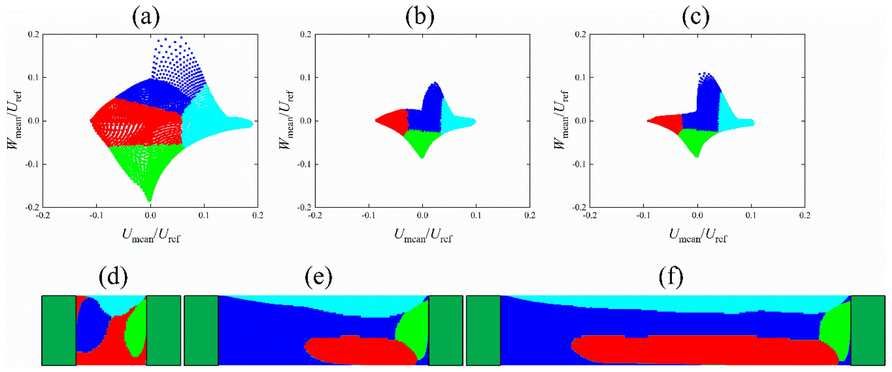
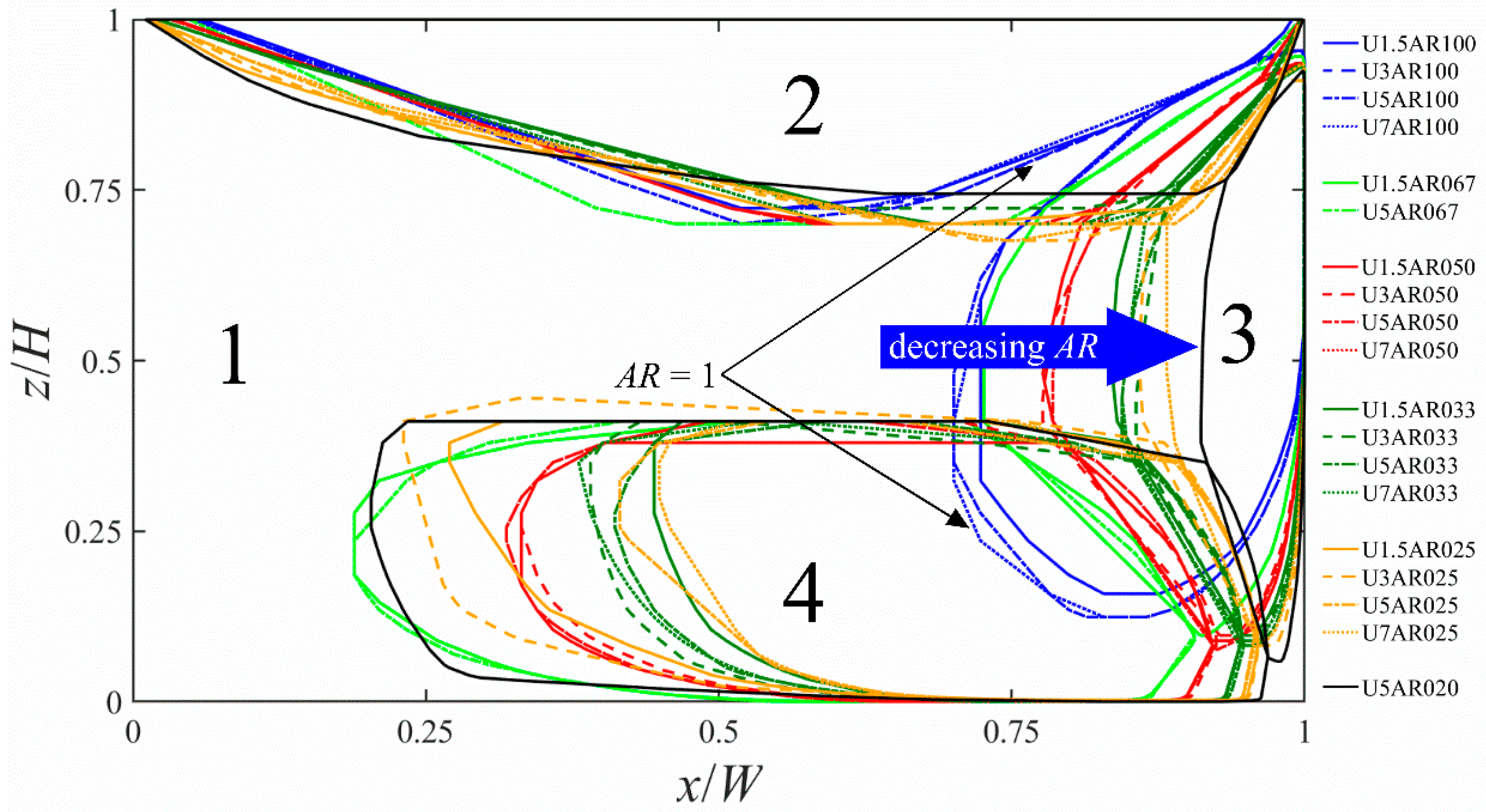
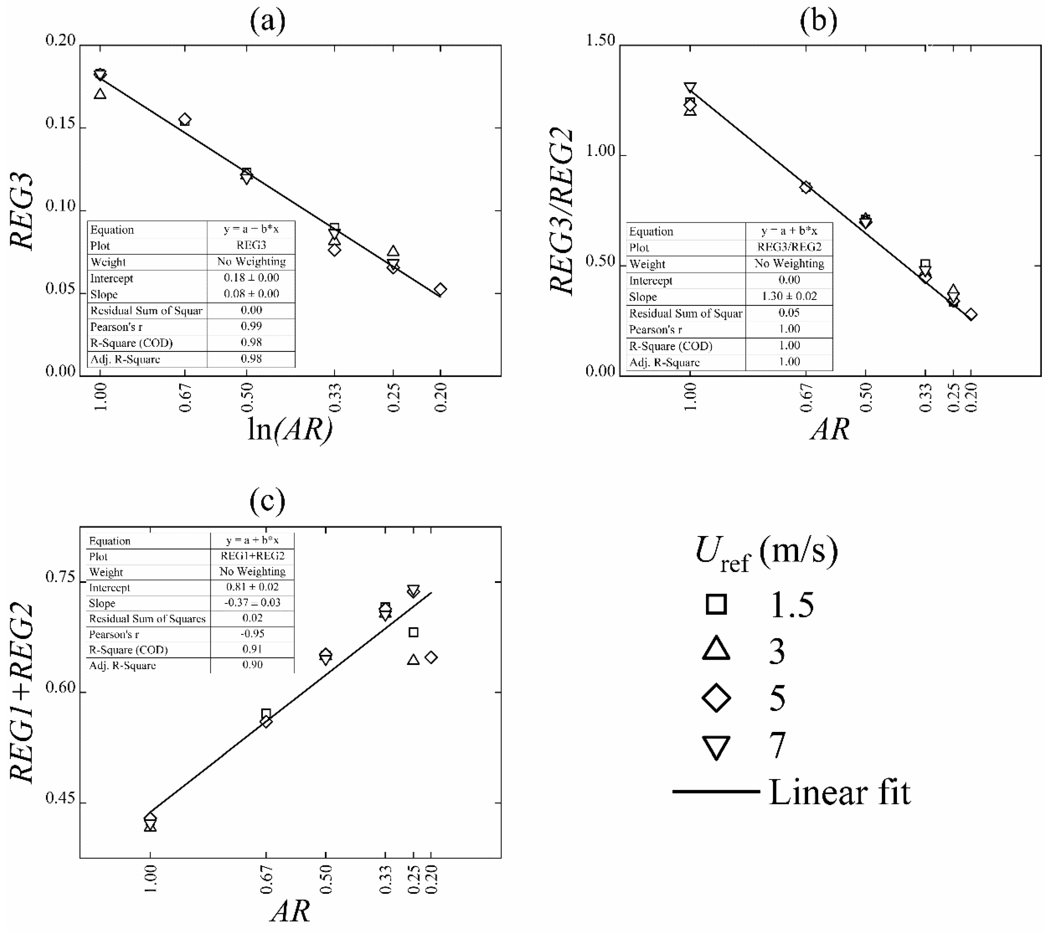
3.2. K-means Clustering

The k–means clustering method was applied for the two main components of the quasi-2D flow, i.e., the horizontal and vertical normalised velocities U_mean/U_ref and W_mean/U_ref. The data observations were collected from each one of the computational cells inside the street canyon area, i.e., less or equal than the building height. The flow along the y-axis (see Figure 1) was examined and found to be similar throughout the domain, so one x-z slice of cells in the middle of the y-axis was selected, at y equal to ~2.5 m out of the total 5 m for this dimension. This resulted to total cells: 14,400 for AR = 1; 21,600 for AR = 0.67; 28,800 for AR = 0.50; 43,200 for AR = 0.33; 57,600 for AR = 0.25; and 72,000 for AR = 0.20. The k-means method requires the clusters’ number to be determined by the user, so trials were conducted with 2, 3, 4 and 5 clusters. The selection of 4 clusters proved to give consistent results and was also selected for a possible comparison with the four events typically recognised in the quadrant analysis method [91].

Figure 4a–c depict the usual scatter plots of the U_mean/U_ref and W_mean/U_ref observations after being classified using the k-means technique. On these charts, each pair of points reflects the calculated U_mean/U_ref and W_mean/U_ref values at a given location on the selected x-z slice (see Figure 1) while arbitrary colours have been used to represent the cluster that each point belongs to. To assist on the interpretation, this information has been transferred to the x-z slice itself (i.e., the physical space) which resulted in Figure 4d–f where each point of the previous figures retains its colouring. In other words, each point on the x-z slice was coloured according to the cluster that it belongs to. From this process, four distinct regions emerge for all the studied cases, representing each created cluster. There are also some smaller detached regions, such as the ones in the lower right side of the canyon in Figure 4e,f. These will be ignored hereafter, for the subsequent application of the regression techniques.

The exact same patterns Figure 4a,d were observed in all cases for AR = 1, i.e., U1.5AR100, U3AR100 and U7AR100. Although the pattern changes for the rest of the aspect ratios i.e., AR = 0.67 up to 0.20 it is again similar in all of them with well-defined oval clusters to occupy the top, right and bottom regions of the street canyon. Noteworthy, the velocities (i.e., Reynolds number) did not have any profound impact on the location and size of the clusters, thus not shown here. The same pictures for U5AR067, U5AR050 and U5AR025 are presented in Figure S2 of the Supplementary Material.

4. Discussion

Previous sections presented the compiled dataset and the outcomes of the main methods employed to analysed it, towards the central hypothesis of this work. That is the implicit definition of the “recirculation zone” and of other characteristic regions inside a street canyon using only information of boundary conditions i.e., buildings’ geometry and prevailing wind. In this context, analysis of the visualization criteria (Section 3.1) could identify the shape of the main vortices by combining the streamlines and λ₂. However, these did not match with the concentration equivalent visualization criteria, because the latter depended heavily on the exact location of the source (simulation and analysis results not shown here). Although, this analysis did not yield quantitative results it strongly indicated that emphasis should be given on the flow characteristics rather than the dispersion characteristics, otherwise, the boundary condition for the source should be considered. Thus, in the remaining of the paper, the study will focus on the analysis of the velocity field.

The k-means methodology (Section 3.2) yielded very consistent results, an example of which is shown in Figure 4d–f. Figure 5 combines the results of the k-means clustering for all 19 combinations of AR and reference velocity using normalised lengths (z/H and x/W). The well-defined boundaries of each identified cluster were extracted using image analysis techniques and arbitrarily numbered from 1 to 4, i.e., 1 for the left, 2 for the top, 3 for the left and 4 for the bottom region. For brevity, the regions of each cluster will be referred as REG1, REG2, REG3 and REG4. Moreover, for the cases with AR = 1, REG1 and REG4 are neglected, because AR = 1 is a special case of street canyons with a singularity concerning the recirculation zone since it is expected to cover the whole canyon.

In more details, REG2 covers the whole shear layer in all cases while its area and shape change very slightly and only to “adapt” to changes in REG3. In contrast, the areas of REG3 and REG4 change drastically following AR changes. Specifically, their shape remains the same, but it shrinks as AR decreases. Noteworthy, both the shape and area of REG3 and REG4 appear independent of the U_ref, except for AR = 0.33 where the REG3 area decreases as the velocity increases.

To take advantage of these observations and of the clusters’ topology remaining constant, the area covered by each cluster was calculated for each studied case, employing the normalised dimensions (with x/W and y/H dimensions), like the ones presented in Figure 4d–f. An exploratory least-squares regression analysis was conducted using AR and U_ref as independent variables and the areas of REG1, REG2, REG3, and REG4 as independent. As expected, the areas showed a strong dependence on the AR of the canyons and a negligible one for U_ref.

Among the different combinations of variables that were tested three obtained the highest correlations (R²): the area of REG3, the ratio of REG3/REG2 areas, and the sum of areas REG1 and REG3. Figure 6 shows these combinations and their dependence on AR. The related linear expressions are:

REG3 = 0.08·ln(AR) + 0.18 (R² = 0.98)

(12)

REG3/REG2 = 1.3·AR (R² = 1)

(13)

REG1 + REG2 = −0.37·AR + 0.81 (R² = 0.91)

(14)

REG1 + REG2 + REG3 + REG4 = 1

(15)

where REG_i (i = 1, 2, 3 & 4) is the region covered by each cluster i in the normalised street canyon with x/W and y/H and total area equal to unity. The first three Equations (12)–(14) come from the studied combinations and the fourth (15) is the overall balance, to guarantee that the total street canyon area remains constant. In the Table S1 of Supplementary Material, we included the rest of the equations with the highest R², which were derived during the search for the appropriate relationships.

Specifically, REG3 matches with the space where the entrainment of cleaner air happens and REG2 corresponds to the shear layer, also regarded as a location with high turbulence. The combination of these two (REG3 and REG2) represents the whole area of the canyon affected by the external wind. Based on the earlier analyses, REG1 and REG4 could also represent some of the other physical phenomena in the street canyon pollutant dispersion. For example, REG4 could represent the street canyon space where a pollutant is traversed and convection dominates. REG1 could represent the space where the pollutant is recycled and turbulent diffusion dominates. Meaning that either REG1 or combined REG1 and REG4, since REG1 engulfs REG4, reflect the overall recirculation zone. This understanding, along with the explicit definition of REG1, REG2, REG3 & REG4 in any street canyon could drastically improve the empirical formulation in street canyon pollution models. Nevertheless, the above formulations need to be tested for more AR (e.g., AR > 1 tall buildings and narrow streets) and most importantly for oblige wind directions.

5. Conclusions

The goal of this study was to derive an implicit or explicit definition for the recirculation zone, an important information for street canyon air quality models. A total of 19 street canyon cases were simulated with LES and transient data (velocity components and concentration) were obtained for AR(=H/W) from 1 to 0.20 and Reynolds number from 960,000 to 4,500,000 and a line pollution source in the middle of each canyon. These simulations cover an important portion of the actual conditions met in street canyons, with the exception of oblique, non-perpendicular wind flows. These data were analyzed with two categories of methods: common visualization criteria, and k-means clustering. Other methods, like the characterization of velocity components as events, according to quadrant analysis, were also tested. They did not contribute to this work and thus not presented herein.

The first two methods were able to qualitatively highlight the flow patterns inside the street canyon but did not yield any quantitative outcomes. For example, the values of λ₂ showed a drop in the power of the main vortex from AR = 1 to 0.2, which is attributed to the velocity resembling the flow of an open field, as the canyon gets wider. Furthermore, the dispersion fields of the scalar pollutant covered the part of the canyon from the pollutant source in the middle up to the upwind building, for all the studied canyons. This did not provide an intuitive division of the street, that could help us identify the recirculation zone and the method was not further pursued.

On the other hand, the k-means technique consistently identified four clusters, each located at a distinct location in the street canyon. The topological information of these clusters matches to some extent the expected physical phenomena in a street canyon. Therefore, the clusters were further analyzed with an exploratory and regression analysis leading to a set of four Equations (12)–(15) that can explicitly define the location and size of each cluster within the canyon. Accordingly, these equations can be used to define the recirculation zone inside street canyons along with other zones of similar interest. In other words, using as input only the AR of a street canyon an AQM can recreate the identified topology (Figure 6), without the need to recalculate the flow field. Furthermore, the four regions can be connected with results of pollutant dispersion fields or of additional correlations, in order to arrive to practical expressions for the pollutant dispersion, as a function of AR.

In comparison to past efforts, (see for example [23,24]) the proposed topology and equations are considered a step forward because they (a) can capture more characteristics of the flow, within a street canyon, than the previous over simplified approaches, (b) require minimum or no user intervention, and (c) could be expanded further to cover other cases and geometries of interest.

At the same time, the latter leads to one of the main limitations of this study that is the lack of more complex street pollution configurations contributing into the regression analysis, like oblique wind directions, heated facades and complicated building envelopes. Moreover, the inclusion of additional aspects will increase drastically the dimensions of the analysis and consequently will become more challenging to extract meaningful and usable expressions. The other and main limitation of this study is the absence of practical testing and evaluation of the proposed approach with the use of an AQM, which will be attempted in the near future. Nevertheless, we believe, that the analysis presented herein can contribute significantly on the improvement of empirical and operational street canyon pollution modelling. In addition, the presented methodology could be employed to understand other or similar systems.

References

1. Requia, W.J.; Adams, M.D.; Arain, A.; Papatheodorou, S.; Koutrakis, P.; Mahmoud, M. Global Association of Air Pollution and Cardiorespiratory Diseases: A Systematic Review, Meta-Analysis, and Investigation of Modifier Variables. Am. J. Public Health 2018, 108, S123–S130. [Google Scholar] [CrossRef] [PubMed]
2. Dominici, F.; Peng, R.D.; Bell, M.L.; Pham, L.; McDermott, A.; Zeger, S.L.; Samet, J.M. FIne particulate air pollution and hospital admission for cardiovascular and respiratory diseases. JAMA 2006, 295, 1127–1134. [Google Scholar] [CrossRef] [PubMed] [Green Version]
3. Bowatte, G.; Lodge, C.; Lowe, A.J.; Erbas, B.; Perret, J.; Abramson, M.J.; Matheson, M.; Dharmage, S.C. The influence of childhood traffic-related air pollution exposure on asthma, allergy and sensitization: A systematic review and a meta-analysis of birth cohort studies. Allergy 2015, 70, 245–256. [Google Scholar] [CrossRef] [PubMed]
4. Raaschou-Nielsen, O.; Andersen, Z.J.; Beelen, R.; Samoli, E.; Stafoggia, M.; Weinmayr, G.; Hoffmann, B.; Fischer, P.; Nieuwenhuijsen, M.J.; Brunekreef, B.; et al. Air pollution and lung cancer incidence in 17 European cohorts: Prospective analyses from the European Study of Cohorts for Air Pollution Effects (ESCAPE). Lancet Oncol. 2013, 14, 813–822. [Google Scholar] [CrossRef]
5. Beelen, R.; Raaschou-Nielsen, O.; Stafoggia, M.; Andersen, Z.J.; Weinmayr, G.; Hoffmann, B.; Wolf, K.; Samoli, E.; Fischer, P.; Nieuwenhuijsen, M.; et al. Effects of long-term exposure to air pollution on natural-cause mortality: An analysis of 22 European cohorts within the multicentre ESCAPE project. Lancet 2014, 383, 785–795. [Google Scholar] [CrossRef]
6. Mahiyuddin, R.; Sahani, M.; Aripin, R.; Latif, M.T.; Thach, T.-Q.; Wong, C.-M. Short-term effects of daily air pollution on mortality. Atmos. Environ. 2013, 65, 69–79. [Google Scholar] [CrossRef]
7. World Health Organization. 7 Million Premature Deaths Annually Linked to Air Pollution. Available online: http://www.who.int/mediacentre/news/releases/2014/air-pollution/en/ (accessed on 12 October 2018).
8. Colvile, R.N.; Hutchinson, E.J.; Mindell, J.S.; Warren, R.F. The transport sector as a source of air pollution. Atmos. Environ. 2001, 35, 1537–1565. [Google Scholar] [CrossRef] [Green Version]
9. Glasius, M.; Ketzel, M.; Wåhlin, P.; Jensen, B.; Mønster, J.; Berkowicz, R.; Palmgren, F. Impact of wood combustion on particle levels in a residential area in Denmark. Atmos. Environ. 2006, 40, 7115–7124. [Google Scholar] [CrossRef]
10. Li, Z.; Feng, X.; Li, G.; Bi, X.; Zhu, J.; Qin, H.; Dai, Z.; Liu, J.; Li, Q.; Sun, G. Distributions, sources and pollution status of 17 trace metal/metalloids in the street dust of a heavily industrialized city of central China. Environ. Pollut. 2013, 182, 408–416. [Google Scholar] [CrossRef]
11. Argyropoulos, C.; Abraham, M.; Hassan, H.; Ashraf, A.; Fthenou, E.; Sadoun, E.; Kakosimos, K. Modeling of PM10 and PM2.5 building infiltration during a dust event in Doha, Qatar. In Proceedings of the 2nd International Conference on Atmospheric Dust—DUST2016, Castellaneta Marina, Taranto, Italy, 12–17 June 2016; pp. 1–6. [Google Scholar]
12. Mayer, H. Air pollution in cities. Atmos. Environ. 1999, 33, 4029–4037. [Google Scholar] [CrossRef]
13. Ng, E. Policies and technical guidelines for urban planning of high-density cities – air ventilation assessment (AVA) of Hong Kong. Build. Environ. 2009, 44, 1478–1488. [Google Scholar] [CrossRef]
14. Wang, J.; Zhao, B.; Wang, S.; Yang, F.; Xing, J.; Morawska, L.; Ding, A.; Kulmala, M.; Kerminen, V.-M.; Kujansuu, J.; et al. Particulate matter pollution over China and the effects of control policies. Sci. Total. Environ. 2017, 584-585, 426–447. [Google Scholar] [CrossRef] [PubMed]
15. Kovar-Panskus, A.; Louka, P.; Sini, J.F.; Savory, E.; Czech, M.; Abdelqari, A.; Mestayer, P.G.; Toy, N. Influence of Geometry on the Mean Flow within Urban Street Canyons—A Comparison of Wind Tunnel Experiments and Numerical Simulations. Water Air Soil Pollut. Focus 2002, 2, 365–380. [Google Scholar] [CrossRef]
16. Dallman, A.; Magnusson, S.; Britter, R.; Norford, L.; Entekhabi, D.; Fernando, H.J.S. Conditions for thermal circulation in urban street canyons. Build. Environ. 2014, 80, 184–191. [Google Scholar] [CrossRef]
17. Saraga, D.; Maggos, T.; Sadoun, E.; Fthenou, E.; Hassan, H.; Tsiouri, V.; Karavoltsos, S.; Sakellari, A.; Vasilakos, C.; Kakosimos, K. Chemical characterization of indoor and outdoor particulate matter (PM2.5, PM10) in Doha, Qatar. Aerosol Air Qual. Res. 2017, 17, 1156–1168. [Google Scholar] [CrossRef] [Green Version]
18. Argyropoulos, C.D.; Hassan, H.; Kumar, P.; Kakosimos, K.E. Measurements and modelling of particulate matter building ingress during a severe dust storm event. Build. Environ. 2020, 167, 106441. [Google Scholar] [CrossRef]
19. Argyropoulos, C.D.; Ashraf, A.M.; Markatos, N.C.; Kakosimos, K.E. Mathematical modelling and computer simulation of toxic gas building infiltration. Process. Saf. Environ. Prot. 2017, 111, 687–700. [Google Scholar] [CrossRef]
20. Argyropoulos, C.D.; Elkhalifa, S.; Fthenou, E.; Efthimiou, G.C.; Andronopoulos, S.; Venetsanos, A.; Kovalets, I.V.; Kakosimos, K.E. Source reconstruction of airborne toxics based on acute health effects information. Sci. Rep. 2018, 8, 5596. [Google Scholar] [CrossRef]
21. Efthimiou, G.C.; Kovalets, I.V.; Argyropoulos, C.D.; Venetsanos, A.; Andronopoulos, S.; Kakosimos, K.E. Evaluation of an inverse modelling methodology for the prediction of a stationary point pollutant source in complex urban environments. Build. Environ. 2018, 143, 107–119. [Google Scholar] [CrossRef]
22. Kovalets, I.V.; Efthimiou, G.C.; Andronopoulos, S.; Venetsanos, A.G.; Argyropoulos, C.D.; Kakosimos, K.E. Inverse identification of unknown finite-duration air pollutant release from a point source in urban environment. Atmos. Environ. 2018, 181, 82–96. [Google Scholar] [CrossRef]
23. Vardoulakis, S.; Fisher, B.E.A.; Pericleous, K.; Gonzalez-Flesca, N. Modelling air quality in street canyons: A review. Atmos. Environ. 2003, 37, 155–182. [Google Scholar] [CrossRef] [Green Version]
24. Holmes, N.S.; Morawska, L. A review of dispersion modelling and its application to the dispersion of particles: An overview of different dispersion models available. Atmos. Environ. 2006, 40, 5902–5928. [Google Scholar] [CrossRef] [Green Version]
25. Eliasson, I. The use of climate knowledge in urban planning. Landsc. Urban Plan. 2000, 48, 31–44. [Google Scholar] [CrossRef]
26. Panagopoulos, T.; González Duque, J.A.; Bostenaru Dan, M. Urban planning with respect to environmental quality and human well-being. Environ. Pollut. 2016, 208, 137–144. [Google Scholar] [CrossRef] [Green Version]
27. Wang, L.; Zhong, B.; Vardoulakis, S.; Zhang, F.; Pilot, E.; Li, Y.; Yang, L.; Wang, W.; Krafft, T. Air Quality Strategies on Public Health and Health Equity in Europe-A Systematic Review. Int. J. Environ. Res. Public Health 2016, 13, 1196. [Google Scholar] [CrossRef] [Green Version]
28. Barlow, J.; Belcher, S. A Wind Tunnel Model for Quantifying Fluxes in the Urban Boundary Layer. Bound.-Layer Meteorol 2002, 104, 131–150. [Google Scholar] [CrossRef]
29. Kastner-Klein, P.; Berkowicz, R.; Britter, R. The influence of street architecture on flow and dispersion in street canyons. Meteorol. Atmos. Phys. 2004, 87, 121–131. [Google Scholar] [CrossRef]
30. Cai, X.M.; Barlow, J.F.; Belcher, S.E. Dispersion and transfer of passive scalars in and above street canyons—Large-eddy simulations. Atmos. Environ. 2008, 42, 5885–5895. [Google Scholar] [CrossRef]
31. Chatzimichailidis, A.E.; Argyropoulos, C.D.; Assael, M.J.; Kakosimos, K.E. A formulation for the street canyon recirculation zone based on parametric analysis of large eddy simulations. In Proceedings of the HARMO 2017—18th International Conference on Harmonisation within Atmospheric Dispersion Modelling for Regulatory Purposes, Bologna, Italy, 9–12 October 2017; pp. 455–459. [Google Scholar]
32. Oke, T.R. Street design and urban canopy layer climate. Energy Build. 1988, 11, 103–113. [Google Scholar] [CrossRef]
33. Berkowicz, R.; Hertel, O.; Larsen, S.E.; Sorensen, N.N.; Nielsen, M. Modelling Traffic Pollution in Streets; National Environmental Research Institute: Roskilde, Denmark, 1997. [Google Scholar]
34. Johnson, W.B.; Ludwig, F.L.; Dabberdt, W.F.; Allen, R.J. An Urban Diffusion Simulation Model For Carbon Monoxide. J. Air Pollut. Control. Assoc. 1973, 23, 490–498. [Google Scholar] [CrossRef]
35. Dabberdt, W.F.; Ludwig, F.L.; Johnson, W.B., Jr. Validation and applications of an urban diffusion model for vehicular pollutants. Atmos. Environ. 1973, 7, 603–618. [Google Scholar] [CrossRef]
36. Yamartino, R.J.; Wiegand, G. Development and evaluation of simple models for the flow, turbulence and pollutant concentration fields within an urban street canyon. Atmos. Environ. 1986, 20, 2137–2156. [Google Scholar] [CrossRef]
37. Li, X.-X.; Britter, R.; Norford, L.K. Effect of stable stratification on dispersion within urban street canyons: A large-eddy simulation. Atmos. Environ. 2016, 144, 47–59. [Google Scholar] [CrossRef] [Green Version]
38. Allegrini, J.; Dorer, V.; Carmeliet, J. Wind tunnel measurements of buoyant flows in street canyons. Build. Environ. 2013, 59, 315–326. [Google Scholar] [CrossRef]
39. Ai, Z.T.; Mak, C.M. CFD simulation of flow in a long street canyon under a perpendicular wind direction: Evaluation of three computational settings. Build. Environ. 2017, 114, 293–306. [Google Scholar] [CrossRef]
40. Berkowicz, R. OSPM—A Parameterised Street Pollution Model. Environ. Monit. Assess. 2000, 65, 323–331. [Google Scholar] [CrossRef]
41. Buckland, A.T. Validation of a Street Canyon Model in Two Cities. Environ. Monit. Assess. 1998, 52, 255–267. [Google Scholar] [CrossRef]
42. Carruthers, D.J.; Holroyd, R.J.; Hunt, J.C.R.; Weng, W.S.; Robins, A.G.; Apsley, D.D.; Thompson, D.J.; Smith, F.B. UK-ADMS: A new approach to modelling dispersion in the earth’s atmospheric boundary layer. J. Wind Eng. Ind. Aerodyn. 1994, 52, 139–153. [Google Scholar] [CrossRef]
43. Cherin, N.; Roustan, Y.; Musson-Genon, L.; Seigneur, C. Modelling atmospheric dry deposition in urban areas using an urban canopy approach. Geosci. Model Dev. 2015, 8, 893–910. [Google Scholar] [CrossRef] [Green Version]
44. Harman, I.; Barlow, J.; Belcher, S. Scalar Fluxes from Urban Street Canyons Part II: Model. Bound.-Layer Meteorol 2004, 113, 387–410. [Google Scholar] [CrossRef]
45. Yang, Y.; Shao, Y. A Scheme for Scalar Exchange in the Urban Boundary Layer. Bound.-Layer Meteorol 2006, 120, 111–132. [Google Scholar] [CrossRef]
46. Soulhac, L.; Salizzoni, P.; Cierco, F.X.; Perkins, R. The model SIRANE for atmospheric urban pollutant dispersion; part I, presentation of the model. Atmos. Environ. 2011, 45, 7379–7395. [Google Scholar] [CrossRef]
47. Soulhac, L.; Mejean, P.; Perkins, R.J. Modelling the transport and dispersion of pollutants in street canyons. Int. J. Environ. Pollut. 2001, 16, 404–413. [Google Scholar] [CrossRef]
48. Cai, X.M. Dispersion of a passive plume in an idealised urban convective boundary layer: A large-eddy simulation. Atmos. Environ. 2000, 34, 61–72. [Google Scholar] [CrossRef]
49. Li, X.-X.; Liu, C.-H.; Leung, D.C. Large-Eddy Simulation of Flow and Pollutant Dispersion in High-Aspect-Ratio Urban Street Canyons with Wall Model. Bound.-Layer Meteorol 2008, 129, 249–268. [Google Scholar] [CrossRef]
50. Zhong, J.; Cai, X.-M.; Bloss, W.J. Modelling segregation effects of heterogeneous emissions on ozone levels in idealised urban street canyons: Using photochemical box models. Environ. Pollut. 2014, 188, 132–143. [Google Scholar] [CrossRef]
51. Lesieur, M.; Métais, O.; Comte, P. Large-Eddy Simulations of Turbulence; Cambridge University Press: Cambridge, UK, 2005. [Google Scholar] [CrossRef]
52. Argyropoulos, C.D.; Markatos, N.C. Recent advances on the numerical modelling of turbulent flows. Appl. Math. Model. 2015, 39, 693–732. [Google Scholar] [CrossRef]
53. Sagaut, P. Large Eddy Simulation for Incompressible Flows: An Introduction; Springer: Berlin, Germany, 2006. [Google Scholar]
54. Yoshizawa, A.; Horiuti, K. A statistically-derived subgrid-scale kinetic energy model for the large-eddy simulation of turbulent flows. J. Phys. Soc. Jpn. 1985, 54, 2834–2839. [Google Scholar] [CrossRef]
55. Yoshizawa, A. Subgrid-scale modeling with a variable length scale. Phys. Fluids A Fluid Dyn. 1989, 1, 1293–1295. [Google Scholar] [CrossRef]
56. Zhong, J.; Cai, X.-M.; Bloss, W.J. Modelling the dispersion and transport of reactive pollutants in a deep urban street canyon: Using large-eddy simulation. Environ. Pollut. 2015, 200, 42–52. [Google Scholar] [CrossRef]
57. Tominaga, Y.; Stathopoulos, T. Numerical simulation of dispersion around an isolated cubic building: Model evaluation of RANS and LES. Build. Environ. 2010, 45, 2231–2239. [Google Scholar] [CrossRef] [Green Version]
58. Assael, M.J.; Kakosimos, K.E. Fires, Explosions, and Toxic Gas Dispersions: Effects Calculation and Risk Analysis; CRC Press: Florida, FA, USA, 2010. [Google Scholar]
59. Issa, R.I. Solution of the implicitly discretised fluid flow equations by operator-splitting. J. Comput. Phys. 1986, 62, 40–65. [Google Scholar] [CrossRef]
60. Weller, H. OpenFOAM: The Open Source CFD Toolbox User Guide; The OpenFOAM Foundation Ltd.: London, UK, 2010. [Google Scholar]
61. Franke, J.; Baklanov, A. Best Practice Guideline for the CFD Simulation of Flows in the urban Environment: COST Action 732 Quality Assurance and Improvement of Microscale Meteorological Models; Meteorologisches Institut Universitat Hamburg: Hamburg, Germany, 2007. [Google Scholar]
62. Lien, F.S.; Leschziner, M.A. Upstream monotonic interpolation for scalar transport with application to complex turbulent flows. Int. J. Numer. Methods Fluids 1994, 19, 527–548. [Google Scholar] [CrossRef]
63. Cai, X. Effects of differential wall heating in street canyons on dispersion and ventilation characteristics of a passive scalar. Atmos. Environ. 2012, 51, 268–277. [Google Scholar] [CrossRef]
64. Chatzimichailidis, A.; Argyropoulos, C.; Assael, M.; Kakosimos, K. Qualitative and Quantitative Investigation of Multiple Large Eddy Simulation Aspects for Pollutant Dispersion in Street Canyons Using OpenFOAM. Atmosphere 2019, 10, 17. [Google Scholar] [CrossRef] [Green Version]
65. Brown, M.; Lawson, R.E.; Decroix, D.S.; Lee, R.L. Mean Flow and Turbulence Measurement around a 2-D Array of Buildings in a Wind Tunnel; US Environmental Protection Agency: Washington, DC, USA, 2000.
66. Li, X.-X.; Leung, D.Y.C.; Liu, C.-H.; Lam, K.M. Physical Modeling of Flow Field inside Urban Street Canyons. J. Appl. Meteorol. Climatol. 2008, 47, 2058–2067. [Google Scholar] [CrossRef]
67. Chew, L.W.; Aliabadi, A.A.; Norford, L.K.J.E.F.M. Flows across high aspect ratio street canyons: Reynolds number independence revisited. Springer 2018, 18, 1275–1291. [Google Scholar] [CrossRef]
68. Kikumoto, H.; Ooka, R. Large-eddy simulation of pollutant dispersion in a cavity at fine grid resolutions. Build. Environ. 2018, 127, 127–137. [Google Scholar] [CrossRef]
69. Schatzmann, M. COST 732 Model Evaluation Case Studies: Approach and Results; Meteorological Institute: Hamburg, Germany, 2010. [Google Scholar]
70. Celik, I.B.; Cehreli, Z.N.; Yavuz, I. Index of Resolution Quality for Large Eddy Simulations. J. Fluids Eng. 2005, 127, 949–958. [Google Scholar] [CrossRef]
71. Jiang, M.; Machiraju, R.; Thompson, D. Detection and visualization of vortices. In The Visualization Handbook; Elsevier: Burlington, MA, USA, 2005; pp. 295–309. [Google Scholar]
72. Chakraborty, P.; Balachandar, S.; Adrian, R.J. On the relationships between local vortex identification schemes. J. Fluid Mech. 2005, 535, 189–214. [Google Scholar] [CrossRef] [Green Version]
73. Jeong, J.; Hussain, F. On the identification of a vortex. J. Fluid Mech. 1995, 285, 69–94. [Google Scholar] [CrossRef]
74. Hunt, J.C.; Wray, A.; Moin, P. Eddies, streams, and convergence zones in turbulent flows. In Proceedings of the 1988 Summer Program, Stanford, CA, USA, 1 December 1988; 1988; CA, p. USA. [Google Scholar]
75. Holmén, V. Methods for vortex identification. Master’s Theses, Mathematics (Faculty of Engineering), Sölvegatan, Lund, 2012. [Google Scholar]
76. Coceal, O.; Dobre, A.; Thomas, T.G.; Belcher, S.E. Structure of turbulent flow over regular arrays of cubical roughness. J. Fluid Mech. 2007, 589, 375–409. [Google Scholar] [CrossRef] [Green Version]
77. Michioka, T.; Sato, A.; Takimoto, H.; Kanda, M. Large-Eddy Simulation for the Mechanism of Pollutant Removal from a Two-Dimensional Street Canyon. Bound.-Layer Meteorol 2011, 138, 195–213. [Google Scholar] [CrossRef]
78. Kellnerová, R.; Kukačka, L.; Jurčáková, K.; Uruba, V.; Jaňour, Z. PIV measurement of turbulent flow within a street canyon: Detection of coherent motion. J. Wind. Eng. Ind. Aerodyn. 2012, 104–106, 302–313. [Google Scholar] [CrossRef]
79. Koutsourakis, N.; Bartzis, J.G.; Efthimiou, G.C.; Venetsanos, A.G.; Tolias, I.C.; Markatos, N.C.; Hertwig, D.; Leitl, B. LES study of unsteady flow phenomena in an urban geometry – the need for special evaluation methods. In Proceedings of the HARMO 2016—17th International Conference on Harmonisation within Atmospheric Dispersion Modelling for Regulatory Purposes, Varna, Bulgaria, 8–11 September 2014. [Google Scholar]
80. Brunton, S.L.; Noack, B.R.; Koumoutsakos, P. Machine learning for fluid mechanics. Annu. Rev. Fluid Mech. 2019, 52. [Google Scholar] [CrossRef] [Green Version]
81. Li, C.; Wang, Z.; Li, B.; Peng, Z.-R.; Fu, Q. Investigating the relationship between air pollution variation and urban form. Build. Environ. 2019, 147, 559–568. [Google Scholar] [CrossRef]
82. Chen, H.; Namdeo, A.; Bell, M. Classification of road traffic and roadside pollution concentrations for assessment of personal exposure. Environ. Model. Softw. 2008, 23, 282–287. [Google Scholar] [CrossRef]
83. Wegner, T.; Hussein, T.; Hämeri, K.; Vesala, T.; Kulmala, M.; Weber, S. Properties of aerosol signature size distributions in the urban environment as derived by cluster analysis. Atmos. Environ. 2012, 61, 350–360. [Google Scholar] [CrossRef]
84. MacQueen, J. Some methods for classification and analysis of multivariate observations. In Proceedings of the Fifth Berkeley Symposium on Mathematical Statistics and Probability; University of California Press: Berkeley, CA, USA, 1967; pp. 281–297. [Google Scholar]
85. Ester, M.; Kriegel, H.-P.; Sander, R.; Xu, X. A density-based algorithm for discovering clusters a density-based algorithm for discovering clusters in large spatial databases with noise. In Proceedings of the Second International Conference on Knowledge Discovery and Data Mining, Portland, Oregon, 2–4 August 1996; pp. 226–231. [Google Scholar]
86. Ward, J.H. Hierarchical Grouping to Optimize an Objective Function. J. Am. Stat. Assoc. 1963, 58, 236–244. [Google Scholar] [CrossRef]
87. Zhang, T.; Ramakrishnan, R.; Livny, M. BIRCH: An efficient data clustering method for very large databases. Proceedings of ACM Sigmod Record, Montreal, QC, Canada, 4–6 June 1996; pp. 103–114. [Google Scholar]
88. Cheng, Y. Mean Shift, Mode Seeking, and Clustering %J IEEE Trans. Pattern Anal. Mach. Intell. 1995, 17, 790–799. [Google Scholar] [CrossRef] [Green Version]
89. Pedregosa, F.; Varoquaux, G.; Gramfort, A.; Michel, V.; Thirion, B.; Grisel, O.; Blondel, M.; Prettenhofer, P.; Weiss, R.; Dubourg, V. Scikit-learn: Machine learning in Python. J. Mach. Learn. Res. 2011, 12, 2825–2830. [Google Scholar]
90. Theodoridis, S.; Koutroumbas, K. Pattern recognition. IEEE Trans. Neural Networks 2008, 19, 376. [Google Scholar]
91. Wallace, J.M.; Eckelmann, H.; Brodkey, R.S. The wall region in turbulent shear flow. J. Fluid Mech. 1972, 54, 39–48. [Google Scholar] [CrossRef]
Figure 1. The quasi-2d street canyon geometry: (a) Physical geometry and boundary conditions; (b) x-z cross-section of the considered computational grid for canyon with AR = 0.50.
Atmosphere 10 00794 g001
Figure 2. Numerical and experimental data for the unity street canyon: (a) average horizontal velocity (Umean/Uref); (b) average vertical velocity (Wmean/Uref); (c) standard deviation of the horizontal velocity (σU/Uref); (d) standard deviation of the vertical velocity (σW/Uref).
Atmosphere 10 00794 g002
Figure 3. Basic flow and dispersion statistics for the street canyons U5AR100, U5AR033 and U5AR020 (left to right): (ac) the average dimensionless magnitude of velocity magUmean/Uref; (df) the λ2 vortex identification criterion; (gi) the normalised concentration Cmean/Cmax; (jl) the dimensionless vertical velocity Wmean/Uref; the street canyon orientation is the same as Figure 1.
Atmosphere 10 00794 g003
Figure 4. Results of the k-means clustering with four clusters, for Umean/Uref and Wmean/Uref, for the street canyons U5AR100, U5AR033 and U5AR020 (left to right): (ac) scatter plots; (df) contour plots; the street canyon orientation is the same as Figure 1.
Atmosphere 10 00794 g004
Figure 5. The combined results of the k-means clustering for all 19 combinations of AR and reference velocity Uref, using normalised lengths (z/H and x/W) with the four clusters denoted.
Atmosphere 10 00794 g005
Figure 6. Selected relations between the area covered by the four regions and the AR: (a) AR and REG3; (b) AR and REG3/REG2; (c) AR and REG1+REG2.
Atmosphere 10 00794 g006