The Mars Regional Atmospheric Modeling System (MRAMS): Current Status and Future Directions

Abstract

The Mars Regional Atmospheric Modeling System (MRAMS) is closing in on two decades of use as a tool to investigate mesoscale and microscale circulations and dynamics in the atmosphere of Mars. Over this period of time, there have been numerous improvements and additions to the model dynamical core, physical parameterizations, and framework. At the same time, the application of the model to Mars (and related code for other planets) has taught many lessons about limitations and cautions that should be exercised. The current state of MRAMS is described along with a review of prior studies and findings utilizing the model. Where appropriate, lessons learned are provided to help guide future users and aid in the design and interpretation of numerical experiments. The paper concludes with a discussion of future MRAMS development plans.

1. Introduction

The Mars Regional Atmospheric Modeling System (MRAMS) is a mesoscale and large-eddy simulation model designed for the simulation of the Mars atmosphere at horizontal scales from O(10 m) to O(1000 km). The development of MRAMS began in the late 1990s. The Mars Pathfinder mission marked the re-ignition of martian exploration after the long, twenty-year hiatus following the Viking missions [1,2]. While the tiny Sojourner rover was blazing the path (and thus, the mission name Pathfinder) for larger and more capable future rovers, the base station lander manifested a compact meteorological station that measured temperature, pressure, and wind [3]. These new data motivated one of us (Rafkin), having initially very little knowledge of the Mars atmospheric literature or Mars in general, to investigate whether anyone had ever attempted to simulate the Mars atmosphere with a mesoscale model. After consulting with colleagues and searching the literature, the answer was clearly “no”, although colleagues thought it would be a worthwhile endeavor. Thus was born the MRAMS project, which was initially supported in the form of a small seed grant by Dr. Robert Haberle at the NASA Ames Research Center, which provided initial, partial funding for MRAMS co-developer Tim Michaels, who was a graduate student at the time. The result of that effort was described in the initial MRAMS paper [4].

The MRAMS model is based on the Regional Atmospheric Modeling System (RAMS) that was in wide use in the terrestrial community in the late 1990s [5]. RAMS version 3b was chosen as the starting point for no other reasons than its familiarity to one of us (Rafkin) resulting from many years of prior use and development for Earth applications, and that was the current stable release at that time. Little to no consideration was given to whether the assumptions that went into RAMS were appropriate for Mars. This was not willful neglect of due diligence, but a reflection of the ignorance of just how differently the Mars atmosphere behaved and was forced, and it would later lead to modifications to everything from model initialization, boundary conditions, the dynamical core, and to the physics that are either unnecessary or inappropriate for Earth applications but are important for Mars. At the same time, however, there was a highly beneficial infusion of terrestrial mesoscale modeling experience and mesoscale dynamics into the nascent Mars mesoscale modeling enterprise. This knowledge would motivate future modeling investigations, influence the interpretation of the results in a broader context of terrestrial analogs, and diffuse to some degree into the more mature global circulation modeling community.

Since the introduction of MRAMS, numerous other mesoscale models have been introduced e.g., [6,7,8]. While all of these models are similar in concept, each has slightly different representations of dynamics (i.e., different dynamical cores) that are solved on different computational grids. The physical representation of Mars processes (i.e., the physics) is generally different. So, while all of these models can generally be applied to similar problems, the answers will generally differ. Further, not all models have the same capabilities within the physics. For example, MRAMS has a bin representation of microphysics that provides the capability for representing complex aerosol size distributions while most other models do not.

The current version of MRAMS is v2.9_r39 and is based on RAMS version 4.4 (c. 2001), with major (nearly all-encompassing) modifications to code structure, the model core, and many physical routines. Although RAMS v4.4 had parallel computing capabilities, that capability was broken as a result of modifications made to apply the model to Mars. Parallel computing capabilities have since been restored, along with greater portability between operating systems and reliability. Below, the details of additions, improvements, and changes are described.

2. Dynamical Core

2.1. Full Compressibility and Buoyancy

RAMS is a nonhydrostatic, but not fully compressible, model. As discussed in [4], sound waves are not filtered but are solved using a time-splitting scheme. Diabatic heating is not fully and properly coupled to the pressure and velocity field. Additionally, to avoid the computationally-expensive need to solve a 3D elliptic equation to obtain the pressure perturbation, the mass continuity equation in RAMS is formulated using the Exner function ($\mathsf{\pi }$) instead of pressure, and linearization of the equations results in the substitution of the time-invariant base-state Exner function (π₀, where $\mathsf{\pi }={\mathsf{\pi }}_0+{\mathsf{\pi }}^{\prime }$ and ${\mathsf{\pi }}^{\prime }$ is the perturbation from the base-state value) for the full Exner function wherever $\frac{{\mathsf{\pi }}^{\prime }}{\mathsf{\pi }}$ appears. This enables a relatively fast tridiagonal solver to be used. In the absence of full compressional heating, the modeled pressure signal using the baseline RAMS dynamical core is unable to faithfully reproduce the strong diurnal pressure cycles of Mars. In the baseline core, heating hydrostatically lowers the surface pressure, but a partially offsetting compressional increase in pressure is necessarily absent or incorrectly diagnosed. The first attempt at rectifying this issue was [9], who found the baseline RAMS dynamical core to be lacking in the case of strong diabatic heating from thunderstorms. For that work, they were able to largely correct this by adding the compressional term (i.e., a term proportional to the time rate of change in potential temperature) to the dynamical core, retaining the same linearization strategy of using π₀ in place of $\mathsf{\pi }$. The same strategy was adopted for MRAMS, which enabled substantially improved simulations of Mars’ diurnal pressure cycles.

In the vertical momentum equation of RAMS, the buoyancy term is approximated as being proportional to the ratio of the potential temperature perturbation to the time-invariant base-state potential temperature (θ‘/θ₀). This is essentially the anelastic approximation. However, linearized buoyancy is properly defined as a mass density ratio (e.g., ρ′/ρ₀), which has an additional term proportional to the linearized Exner function ratio ($\mathsf{\pi }$′/π₀). MRAMS now includes the Exner function term, which necessitated the re-derivation of matrix coefficients for the implicit tridiagonal solver.

The inclusion of the additional compression and buoyancy terms can generally cause some energy non-conservation and inconsistencies in the equations, but these were found to be acceptable in practice, particularly since the lack of inclusion made the realistic simulation of atmospheric tides and other circulations on Mars impossible. Since MRAMS is a limited area model run over relatively small timescales (e.g., less than 10 sols), long term non-conservation is not as much a concern as it would be in a global climate model.

2.2. The Pressure Cooker Effect

MRAMS uses a terrain-influenced, geometric (not pressure) height coordinate. The lowest model levels follow the topographic relief and gradually relax to a purely horizontal surface at the model top. Typically, the lowest model level thickness is set to 10 m to 30 m and is gradually stretched to a spacing of ~2 km up to a model top of >50 km. The upper boundary condition is w = 0 (vertical velocity), as described in [4]. The inclusion of full compression in a rigid lid, height-based model is not without issues. Consider a global model with domain boundaries at the surface and a model top at a specified geometric height. Assuming w = 0 boundary conditions at both the top and bottom of the model and no other sources of mass, the domain mass in the model is fixed. Now suppose the global domain is heated such that the mean temperature increases. From the Ideal Gas Law, the heating in the fixed volume will result in a compressional increase in pressure, including at the surface. Normally, however, the surface pressure is considered to be a diagnostic of the total column mass (to within hydrostatic accuracy). The model domain mass has not changed during the heating (the mass is fixed) while the surface pressure has. The domain mass and the surface pressure have decoupled so that the model surface pressure cannot be used as a diagnostic for atmosphere mass.

The decoupling of the surface pressure from the domain mass is because of the upper rigid lid boundary condition in a model atmosphere of finite depth. When heated, the atmosphere should be able to expand upward to alleviate some or all of the compressional pressure increase. It is unable to do so, and thus the pressure field must absorb all the heating via compression. Further, the model has no knowledge of the atmosphere above the rigid lid. The implicit assumption is that the atmosphere above the model has no impact or influence on the atmosphere below. Effectively, the atmosphere above may be considered static such that the pressure (i.e., the mass above) is invariant. This sets up a discontinuity between the pressure at the top of the model inside the model domain and the pressure just on the other side of the domain. Notably, models with vertical pressure coordinates and fixed pressure upper boundary conditions can expand vertically and can properly deal with the compressional heating.

The compressional decoupling of mass and surface pressure in rigid lid z-models has been known in the Earth modeling community for some time e.g., [10]. It is generally ignored because the heating of the Earth’s atmosphere is generally small enough such that the discrepancy is small. Further, Earth models are usually started from close to a thermal equilibrium state such that secular changes in global temperature are small. This is not the case for Mars global models where the atmosphere is usually started from an isothermal state far from the final thermal equilibrium state. In the case of Mars, the global surface pressure can deviate substantially from the initial value due solely to changes in the mean thermal state with absolutely no change in domain mass. The noticeable compressional pressure effect on Mars has been termed the “pressure cooker” effect (possibly first coined by R. Haberle).

Although MRAMS is not a global model, it can still suffer from the pressure cooker effect. A locally heated column cannot expand vertically beyond the model top. The column heating drives a horizontally divergent (expansive) flow with the balance of the heating producing some amount of compressional pressure increase. The partitioning will depend on the specific formulation of the model core and its handling of acoustic waves in particular. Regardless, it is reasonable to assume that there is some amount of spurious lateral flow and spurious compressional pressure signal. These spurious flows are superimposed on realistic lateral flows (e.g., the thermal tide) and compressional tendencies. Some lateral flow is correct. This divergence is, after all, what produces a thermal low pressure in response to heating.

The pressure cooker effect in MRAMS is noticeable in spin up when the model is initialized with a General Circulation Model (GCM) field that is not in close thermal equilibrium with the end state. A secular trend in pressure is common for one or two sols after initialization. The signal is domain-wide and has not been found to have a noticeable impact on winds or temperature. Winds are driven by pressure gradients, so the minimal impact must indicate the pressure cooker forcing is nearly uniform over the domain. Temperature is largely driven by radiative forcing, and while there is some pressure dependence on this forcing, it is very small over the range of typical spin-up scenarios (<2% domain change in pressure). The diurnal (tidal and local circulation) pressure changes are much larger and are superimposed on the spin-up signal.

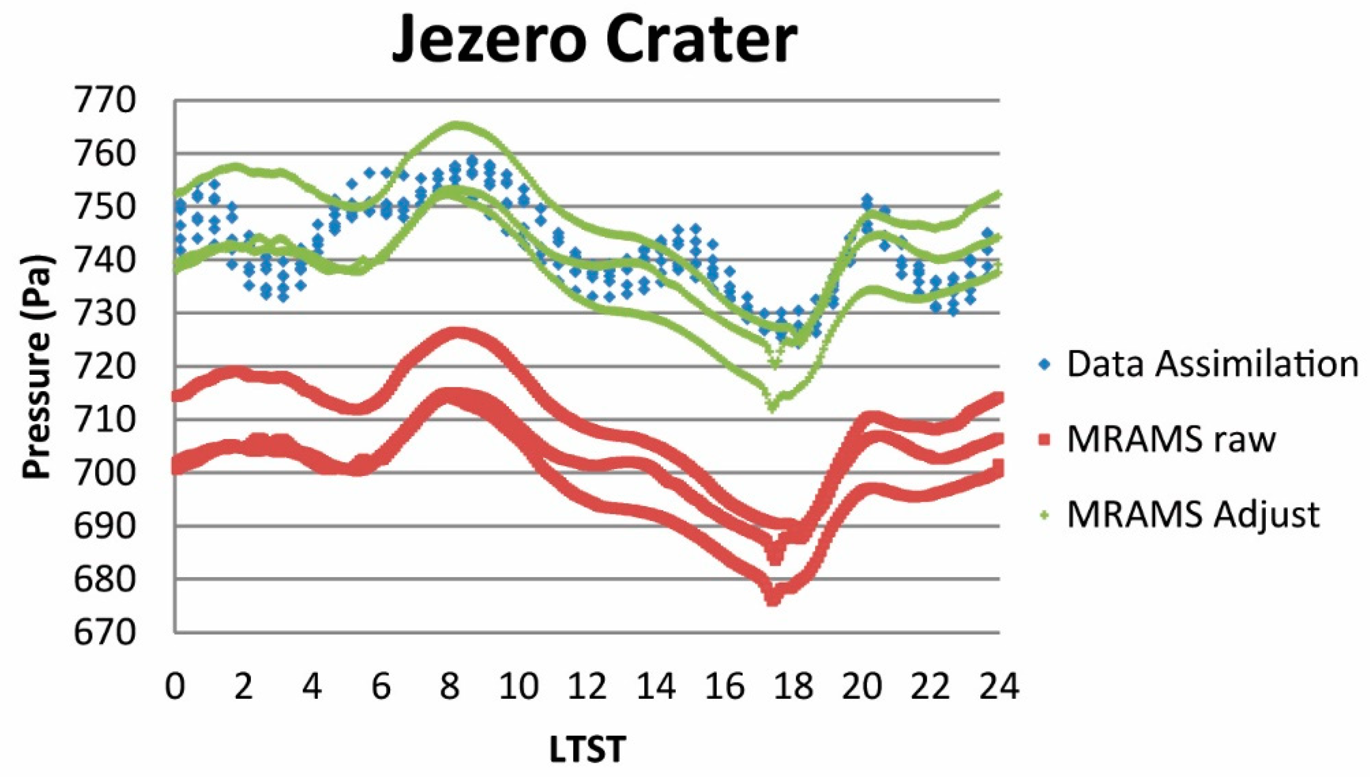
The ability of MRAMS to reproduce observed variations in pressure [11] suggests that spurious lateral flows and column compressional pressure changes must be small enough in combination such that the real dominant tidal signatures plus local, topographically-driven circulations shine through [12]. This has never been properly confirmed. MRAMS can have a difficult time reproducing the mean pressure without either adjusting the initial state with a posteriori information or adjusting the mean pressure in the post-simulation analysis. In the first case, the quasi-equilibrium solution is used to determine a domain-wide, constant scaling factor by which the initial input pressure field (and boundary condition data) from the large-scale model is adjusted so as to equal the desired, observed mean pressure. Then MRAMS is re-run with the corrected initial and boundary conditions so that the modeled mean pressure relaxes close to the desired, observed value. In the second case, the output pressure field from the initial MRAMS simulation is corrected post facto in the analysis by the scaling factor, and no additional simulations are conducted. Tests between these two methods have shown that the difference in solutions is inconsequential. Thus, for most cases, the second method is used in order to minimize computation.

Figure 1 displays an example of the pressure correction method that was applied to simulations conducted in support of entry, descent, and landing (EDL) engineering activities for the NASA Mars 2020 rover. MRAMS is capable of characterizing the variations in density, winds, and temperature, but the mean density and pressure are not constrained by MRAMS alone. An independent study using MGS Radio Science as input into a data assimilation simulation with the UK version of the Laboratoire de Météorologie Dynamique, or LMD Mars GCM was used to compute the mean diurnal pressure [13].

Deep atmospheric domains should, in principle, help to offset the pressure cooker effect, because a large volume produces a relatively small pressure response for a given temperature change. Further, a model top at low pressures should mean that the assumptions about the atmosphere above the model become less important. Fortunately, the deep circulations on Mars require deep model domains, but the response of the pressure cooker effect to changes in the model top has not been documented in the literature. Next-generation model development efforts that use a rigid z-lid should be aware of and will have to deal with the pressure-cooker effect.

3. Nested Grid Feedback

The default, two-way nesting scheme in RAMS is described by [14] and is based on a reversible and conservative methodology of the primary prognostic variables, namely ice-liquid potential temperature (θ_il) and the Exner function (π). The ice-liquid potential temperature in MRAMS is set equivalent to potential temperature since the amount of water is thermodynamically small. The average of these two atmospheric properties taken over the child grid cells contained within a single parent grid cell determines the up-scale value of the parent grid cell. Thus, $\overline{\theta }=\sum {\theta }_{ij}/N$ and $\overline{\pi }={\sum }^{ }{\pi }_{ij}/N$, where the sum is performed over the N child grid cells ij contained with the parent cell. Parent grid temperature is diagnosed from the prognostic thermodynamic variables, $C_p\overline{T}=\overline{\pi }\overline{\theta }$. The temperature in the parent cell is then $\overline{T}=\sum {\pi }_{ij}\sum {\theta }_{ij}/(N^2{C}_p)$ while the average temperature of the child cells is $\sum {\pi }_{ij}{\theta }_{ij}/\left(N{C}_p\right)$.

The baseline feedback process can produce a diagnosed temperature in the parent grid cell that differs from the average temperature over the child cells. When topography is added, the discrepancy can be amplified, because even if potential temperature is conserved, the resulting temperature depends on altitude. On Mars, this effect can and often does produce non-physical values of temperature in the parent grid cell in regions of extreme topography. For example, over the Tharsis Montes, the variation of topography within child grid cells can be several kilometers with pressure values varying accordingly. We often found that the diagnosed parent grid air temperatures in these steep topography scenarios could exceed 340K or drop well below the CO₂ condensation temperature after feedback from the child grid with reasonable temperatures. The potential temperatures of parent and child grid values were compatible, but the very different altitudes of the parent and child grids produced incompatible temperatures. These temperatures then triggered incorrect dynamical and physical responses such as cloud condensation or bizarre thermal slope flows. On occasion, they could produce numerical instabilities that would bring the model down. While this effect is necessarily present in RAMS, the far tamer Earth topography and thermal structure mute the signal to apparently acceptable levels.

In principle, the nonphysical parent grid solutions can be ignored since they are overwritten by the solutions from the child grid cells at the next time step. However, the nonphysical parent grid solutions can produce gravity waves that may propagate beyond the edge of the nested grid, as can cloud condensate. Also, the child grid utilizes parent values at the grid boundary and vice versa, which can result in substantial discontinuities. Thus, the overall solution may become contaminated. If nothing else, analyzing the parent grids’ solutions in regions of nested grids becomes impossible due to the spurious values resulting from linear averages.

One solution to this problem is to feedback density-weighted prognostic variables and then normalize those variables by the parent grid=density. In the current version of MRAMS, the parent grid values are now defined as $\overline{\theta }={\sum }^{ }{\rho }_{ij}{\theta }_{ij}/\left(N\overline{{\rho }_o}\right)$ and $\overline{\pi }=\sum {\rho }_{ij}{\pi }_{ij}/\left(N\overline{{\rho }_o}\right)$. This formulation normalizes the average child properties to a value consistent with the parent grid density. The prognostic momentum variables are also fed back by weighting with the child base state density (i.e., momentum rather than velocity), and restored to velocity components on the parent grid using the parent grid base-state density. This ensures that momentum is conserved. [15] was the first result published using the new scheme, and that study was only possible with the modified feedback scheme.

4. Physical Parameterizations

4.1. Dust and Dust Lifting

The radiative impact of dust is a crucial element of Mars atmospheric simulation. Two dust fields are now carried in the model: foreground dust and background dust, as described below. Dust lifting, sedimentation, and cloud condensation (i.e., microphysics; see 4.2) operate only on the foreground dust field.

4.1.1. Foreground and Background Dust

MRAMS 2001 utilized a simple background dust field that interfaced directly with the two-stream radiation code originating from the NASA Ames GCM available at the time [16]. The dust distribution was described via total column opacity at the 610 Pa level and followed a Conrath-ν vertical profile [17]. Below the 610 Pa level, the dust was assumed to be well-mixed and constant in mixing ratio. The column opacity was user-specified (as a constant), as were Conrath-ν parameters. Optical parameters for the dust (e.g., single scattering albedo and the visible-to-infrared albedo ratio) were fixed.

By the early 2000s, MGS-TES retrievals of total column dust opacity provided the means to initialize the background dust field with more complex and realistic distributions [18]. A zonally-averaged opacity map that mimicked the bulk properties of the TES data, which varied with season, was implemented around 2004. The opacity fields were combined with Conrath-ν parameters that also varied with latitude and season; deepest dust was prescribed near the subsolar point in a manner consistent with prior studies [19,20,21]:

$$\Delta {\mathrm{L}}_{\mathrm{s}}={\mathrm{L}}_{\mathrm{S}}-{240}^{°}$$

(1)

$$\gamma =0.023{\left|\sin \left(\Delta L_s\right)\right|}^{1.5}+0.007$$

(2)

$$\nu =0.04-\left(0.04-\gamma \right)\cos {\left(\theta \right)}^{0.75}$$

(3)

where $L_S$ is the season of interest, $\theta$ is the latitude, and $\nu$ is the traditional Conrath-ν parameter as described in [17]. A similar zonally-averaged map derived directly from TES Mars Year 24 was also added around that time, and this map was combined with the vertical distribution profiles suggested by the ESA Mars Express SPICAM dust retrievals [19]. The possibility for the user to create a custom opacity map with minor changes to the portion of the code that filled the 2D opacity array was also implemented. All of these options are still available in the current model.

The desire to simulate the dust cycle with dust lifting, sedimentation, advection, diffusion, and volatile condensation on dust as nuclei drove the development and inclusion of a secondary dust field—the foreground dust—within the model. The foreground dust field is represented via dust bins discretized by particle mass. Besides allowing for a more realistic representation of dust cycle processes, the number concentration of dust as a function of the discretized size bins also provides information to more advanced radiation transfer parameterizations that explicitly make use of the information. The number of bins and their discretization are user-defined at the start of the simulation. The foreground dust field can be initialized in the same way as the background dust, or it can be initialized to zero. Unlike the background dust field, however, the foreground dust field evolves based on physical dust processes, with the individual size bins acting independently. For example, the dust in the larger size bins falls more rapidly than in the smaller size bins, leading to a depletion of dust in the larger size bins over time.

The background and foreground dust fields are used individually or in combination to simulate a wide variety of scenarios. For example, one common implementation is to use the background dust field to represent the climatological dust distribution and then use the foreground dust to simulate positive perturbations on that climatological background. This scenario is useful for simulating dust devils or larger dust storms that result from active dust lifting on a pre-existing (background) atmospheric dust distribution. When interfacing with the radiative transfer physics, the total dust (foreground plus background) can be sent as input. In this case, the user must specify the size distribution and vertical distribution of the background field. This configuration scenario was used in [15] to simulate the spiral dust cloud above Arsia Mons. The spiral cloud was represented entirely in the foreground dust field.

The radiative transfer activity of the foreground dust can be toggled on and off. This permits the investigation of the forcing associated with the positive dust perturbations. For small positive dust perturbations (less than ~0.1 additional column opacity), the impact of the foreground dust on the model solution tends to be small, but there are exceptions. Positive dust perturbations result in heating perturbations that hydrostatically lower surface pressures, which then accelerates winds, which can lead to further dust lifting and reinforcement of the heating. The magnitude of this wind-enhanced interaction of radiation and dust (WEIRD) varies [22]. Also, it matters how the foreground dust is distributed vertically. The thermal impact of a small amount of dust spread deeply through the atmosphere is inconsequential, whereas that same amount of dust concentrated in a shallow layer can result in a notable thermal influence in the dusty layer. Generally, for dust perturbations greater than ~0.1 in column opacity, the radiative impact of the additional dust is almost always found to be important.

4.1.2. Dust Lifting Physics

Dust lifting comes in two flavors and only contributes to the foreground dust field. The fairly standard threshold lifting scheme e.g., [23] was the first to be included in the model. In this formulation, only the resolved wind acts on the dust with a lifting threshold and lifting efficiency factor that are specified by the user. These values are set domain-wide, although fairly simple modifications within the code permit the user to provide spatially-variable values, if desired. There is no sub-grid scale dust devil lifting, which is also implemented in some models e.g., [24].

A second parameterization assumes a sub-grid Weibull wind distribution centered on the model-predicted wind speed in the grid cell [25]. The width of the distribution depends on stability (i.e., convective/unstable, neutral, stable) with the convective distribution assumed to be the most turbulent and, therefore, the widest. In contrast, stable conditions are more likely to produce quasi-laminar, narrow distributions. Given the distribution, the winds above a specified lifting threshold may be calculated, and this information is used to diagnose when lifting occurs and in what amount. Thus, it is possible for the modeled winds to remain below the lifting threshold while dust is still lifted due to the stronger sub-grid scale winds in the tail of the Weibull distribution. In this way, dust devil lifting and lifting by other sub-grid scale processes that are represented in the high wind speed tail of the distribution may be captured without the need for a separate, stand-alone parameterization.

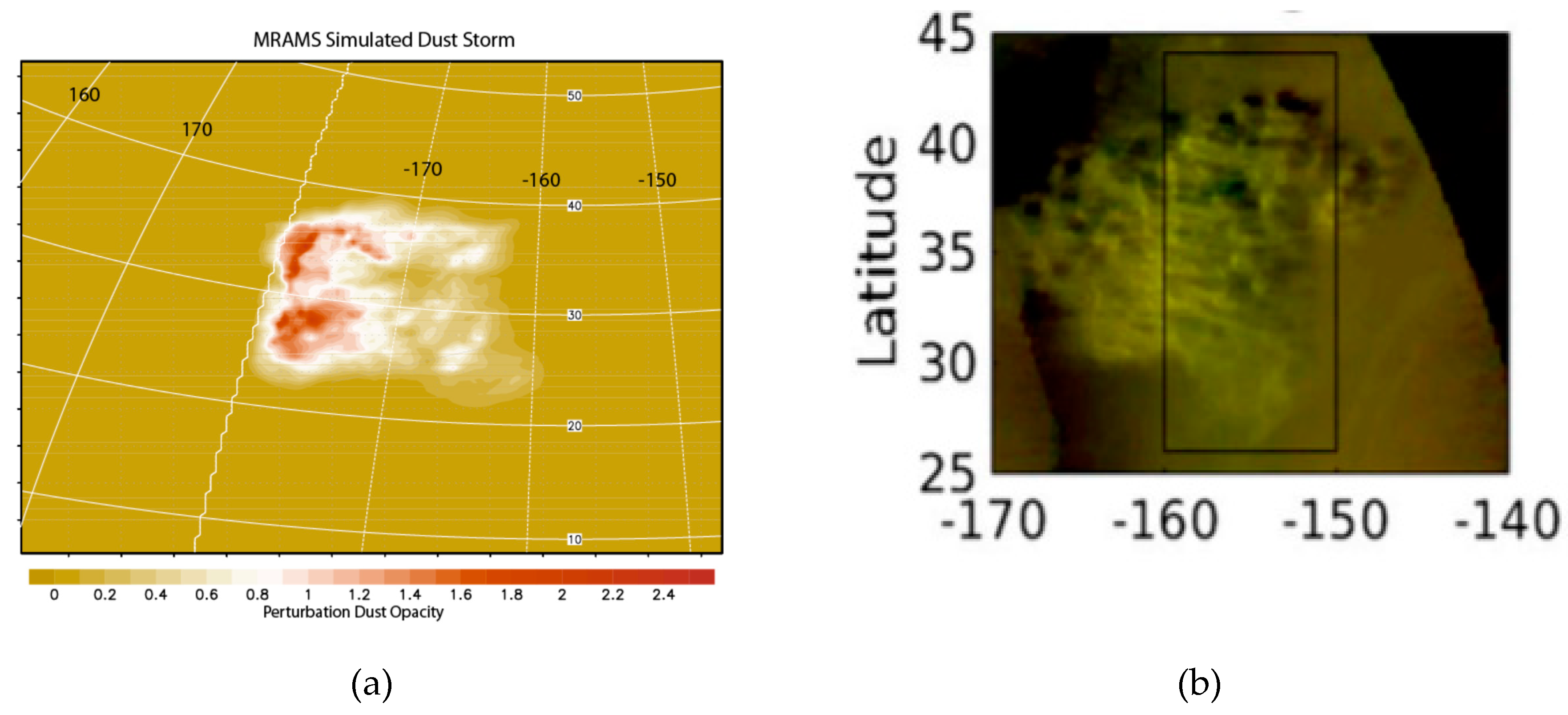
Both lifting parameterization options require the specification of poorly constrained parameters. In practice, the values are set through an iterative process, with the user examining the output from an initial simulation, adjusting the parameters up or down to drive the resulting dust field toward the desired result, and re-running the simulation. For example, [26] simulated a dust storm in Isidis Planitia, but in order to achieve dust opacities that were representative of typical storms, over a dozen simulations had to be conducted in order to appropriately tune the unknown lifting parameters. Similarly, by tuning dust lifting parameters, it was possible to generate a dust storm that was morphologically similar to the storms found in the region of Northeast Amazonis/Southwest Arcadia (Figure 2), as described by [27].

4.2. Cloud Microphysics

To enable detailed Mars cloud simulations with MRAMS e.g., [28], a suitable cloud microphysics scheme was needed. The eventual choice was the Community Aerosol and Radiation Model for Atmospheres (CARMA) model [29] adapted for Mars H₂O ice and CO₂ ice clouds as in [30,31]. A monodispersed or bulk (moment) microphysical model e.g., [32,33] was not chosen, because of the inherent limits of an analytical distribution to represent complex size distributions that might be important for Mars. CARMA discretizes the mass (size) distributions of airborne dust, H₂O ice, and/or CO2 ice particles into a user-specified number of bins with a user-specified width (e.g., eight dust bins from 0.05–5 mm; 18 H₂O ice bins from 0.07–102 mm). All modeled particles are subject to the full range of atmospheric transport, including sedimentation/precipitation in a non-zero vertical velocity environment and turbulent mixing. Sedimentation/precipitation is calculated by the CARMA-based routines, while particle advection and turbulent diffusion time rates of change are calculated by the MRAMS dynamical core and applied by the microphysical driver routine. H₂O ice is permitted to heterogeneously nucleate on or sublimate from foreground dust particles. CO₂ ice is permitted to heterogeneously nucleate on or sublimate from either foreground dust particles or H₂O ice particles. MRAMS also tracks the number/amount of airborne particles that fall to the ground, and the fallen dust may be optionally lifted again by turbulent wind gusts. Using the CARMA microphysics in MRAMS is computationally-intensive compared to a moment-based method. However, it has enabled MRAMS to simulate complex phenomena such as multimodal cloud particle size distributions in the lee clouds of the Tharsis Montes [28] and dust devil track generation [25].

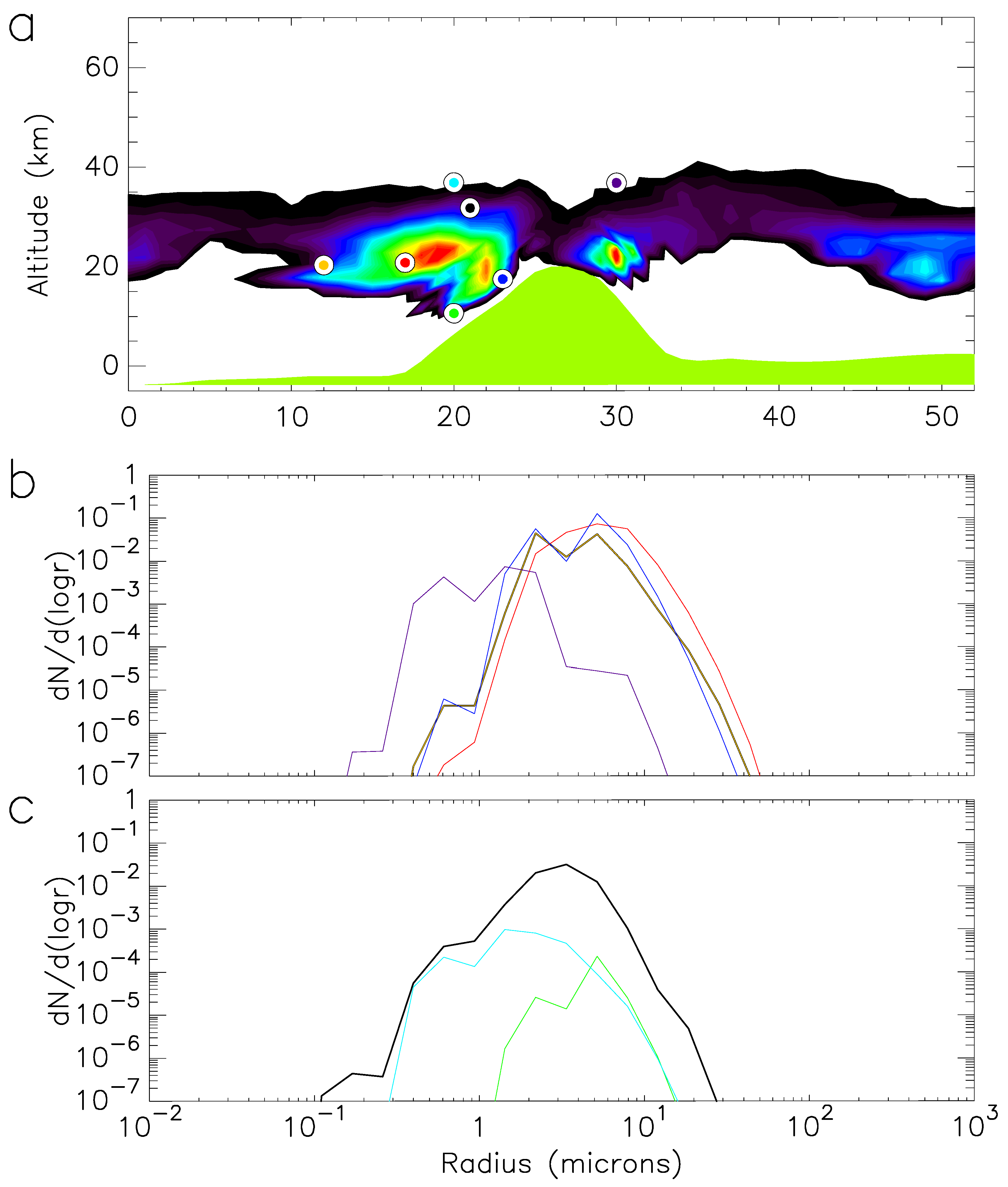
An example of the modeled microphysical details of the afternoon clouds associated with Olympus Mons is given in Figure 3. These clouds are due to thermally-induced upslope flow transporting water vapor and dust along the flanks of the volcano from lower levels. The adiabatically cooled air produces a primary cloud particle growth region in the lee of the mountain. Rapid growth results in narrow distributions of water ice particles with relatively large effective radii (r_eff ~8 µm) in the lee of Olympus Mons. As they form, these particles are transported downstream (to the west) and out of the updraft core by the large-scale horizontal winds. A substantial portion of the cloud mass quickly falls to lower elevations above the flank of the volcano (the larger particles have fall velocities near 1 m s^-1), but the smaller particles have settling times long enough to create a cloud “plume” oriented in the downstream direction, which elongates with time. A wide variety of cloud particle populations is present in the model results, as shown in Figure 3. Preferential sedimentation of large particles results in size sorting within the “plume” such that the effective radii of the condensate particles generally decreases with both height and lateral distance from the volcano. The simulated cloud particle radii and relatively broad size distributions are consistent with telescopic observations of the afternoon clouds over the Elysium Mons volcano [34]. Rapid, often violently turbulent transport of diverse water-ice particle distributions (especially in the lee, just above and below the most massive portions of the cloud) creates multiple regions of bimodal particle distributions. The simulated particle size and spatial distributions are clearly in conflict with simple microphysical representations used in some models, and also with spectrometer retrievals of the aerosol effective radius that assume particle sizes are constant with height e.g., [35]. Therefore, the magnitude of the effect of these possible significant spatial and temporal variations of aerosol size distributions should be considered when interpreting radiance-derived and model-predicted fields that are based on simpler assumptions about the aerosol size and spatial distributions.

4.3. Radiative transfer

There are now three radiative transfer options currently available, while only one was available in 2001. The new options use a two-stream correlated-k method [36] or an implementation of the DISORT discrete ordinates method [37]. One of the last two options must be used when the foreground dust is active or if microphysical species are selected to be radiatively active.

Radiative transfer calculations are computationally demanding, often requiring one or even two orders of magnitude more time than the dynamical core calculations. Taking advantage of the fact that over short time intervals the radiative transfer solution (e.g., heating rates, radiative fluxes) does not change much, the radiative transfer is generally not calculated every dynamical core timestep in an MRAMS run. Instead the radiative transfer solution is computed only every radiative transfer timestep (usually set at ~300 s for mesoscale runs and ~30 s for microscale experiments), and this fixed forcing is applied repeatedly during the often much shorter dynamical timesteps.

During the implementation of the DISORT option, a coding bug affecting the correlated-k scheme was discovered and fixed. The bug had the effect of producing slightly erroneous heating rates over a narrow range of column opacities between ~1 to 3. The bug does not affect any prior published results in any significant way to the best of our knowledge.

4.3.1. Pollack Two-Stream

The original radiation scheme in MRAMS was adapted directly from the scheme present in the stable version of the NASA Ames Mars general circulation model available at the time [38]. As described in [4], that code uses look-up tables to determine the net solar flux as a function of pressure and opacity. Infrared forcing is split into two bands: the 15 mm CO₂ emission region and wavelengths outside that region. Column opacity is fixed, and a Conrath-ν profile is assumed [17]. That original radiation parameterization is still available in the model, although it is now rarely used.

4.3.2. Correlated-k

The correlated-k radiative transfer option is based on the CARMA radiative transfer code [36] and is a two-stream plane-parallel scheme. Gas opacities are calculated using the correlated-k approach with coefficients for CO₂+H₂O mixtures, using the same spectral intervals as the most current version of the NASA Ames Research Center GCM radiative transfer code [39]. Separate mass/size distributions of foreground and background airborne dust may be used with the restriction that they must use the same dust mass/size bin discretization as the CARMA microphysical parameterization (see Section 4.2). Additionally, the radiative transfer effects of airborne water ice and CO₂ ice particles can be calculated with this scheme. As described for dust in Section 4.1.1, the radiative transfer contribution of each foreground airborne particle type (dust, H₂O ice, and/or CO₂ ice) can be individually toggled on or off.

Optical properties, as a function of particle radius and radiation wavelength, of H₂O ice particles are derived with a Mie code [40] and standard refractive indices [41], assuming sphericity. Optical properties of CO₂ ice particles are derived with the same Mie code and refractive indices from [42,43], assuming sphericity. Optical properties of dust particles are also derived using that Mie code, assuming sphericity, but one of three sets of published refractive indices may be selected. Two of these dust refractive index options are based on the optical properties of palagonite: 1) values from the ultraviolet to a wavelength of 4.23 µm [44], values from 4.23 µm to 24.88 µm [45], and 2) values from ~0.2 µm to 24.88 µm [45]. Both use a power-law dependence (λ^–0.25; as in [46]) at longer wavelengths. The third dust refractive index option uses values derived from spacecraft observations of Mars dust from the ultraviolet to ~98.5 µm [47], with the same power-law dependence (λ^–0.25) at longer wavelengths.

4.3.3. DISORT

The ability to use the DISORT radiative transfer parameterization was recently contributed by Dr. Hao Chen-Chen from the University of the Basque Country. DISORT assumes a plane-parallel atmosphere and solves the radiative transfer equation with multiple scattering over a specified number of streams using the discrete ordinates method [48]. The default in MRAMS is eight streams and can be increased up to a maximum value of 32. A key difference between DISORT and the two-stream codes is the use of dust phase function moments expressed as Legendre polynomials. In each wavelength band (i.e., stream), there are 16 quadrature points, each of which is represented by a 32-degree polynomial. The values are derived from [47].

Some additional helpful features were added during the implementation of DISORT. Firstly, the ability to reference the opacity to the surface pressure rather than a hardwired 610 Pa reference level was added. The code for the 610 Pa reference is still active and is the default setting, but it can be easily overridden by a toggle in the source code. This feature is likely to become a toggle available as an option in the namelist in future versions. Secondly, the ability of the user to more easily prescribe an arbitrary vertical dust distribution profile is now included in the source code. As a result, prior calculations that assumed a Conrath-ν shape have been generalized.

4.3.4. Topographic Effects

The use of topography in MRAMS brings up a need to consider its effects on the amount of radiation incident upon (or emitted from) the sloped surface of each horizontal grid cell. This is particularly important for downwelling shortwave radiation due to its primarily direct-beam (as opposed to omnidirectional) nature. MRAMS can be configured to take slope angle and orientation and/or horizon obstruction/extension into account—or simply assume all grid cells are flat for the purposes of radiative transfer only.

Slope angle is the vertical angle between the surface and a horizontal plane, and slope orientation (or aspect) is the horizontal circular angle between north and the direction the slope faces. The more directly a sloped surface faces a beam of radiation, the more radiative flux it will receive (and vice versa). For example, if the sun is directly to the south at an elevation angle of 40°, an unobstructed south-facing 40° slope would receive significantly more insolation than either a flat surface or a NW-facing sloped surface (or indeed, any other sloped surface). If their use is desired, during initialization, MRAMS calculates (and saves for runtime use) the slope angle and orientation values for each horizontal grid cell from the finalized topography field for that grid. At runtime, a standard trigonometric expression (dependent on orbital parameters, time, and geographic location) is used to calculate the factor which, when multiplied by the incoming radiative flux, specifies the flux incident upon the sloped surface.

In the case of zero topography, the horizon would be 90° from vertically straight overhead (Z_h; horizon zenith angle) in all directions. This is not the case with realistic (generally non-zero) topography, where the horizon may also be obstructed (i.e., Z_h < 90°; resulting in the surface being shadowed part of the time) or extended (i.e., Z_h > 90°; resulting in the surface receiving enhanced illumination before sunrise or after sunset). Note that horizon obstruction/extension is not a parameter that can be calculated using a single grid cell’s information, but instead requires taking the planet’s curvature and relatively distant topography into account. If this option is desired, during model initialization, a process akin to ray-tracing is used to determine the circular “viewshed” (Z_h profile discretized into 48 regular angular bins) around each grid cell and saves these for use during the run. For each viewshed bin, a modified 400 km long radial topographic profile (chosen to account for the greatest topographic relief on Mars) is constructed, subtracting the planet’s curvature from the usual topography values. Note that all topographic information used in this process is prepared just as the regular MRAMS topography is. This modified topographic profile is then used to determine the Z_h (as well as the lateral distance to and apparent height of an obstruction) for that viewshed bin. The process is repeated for the other viewshed bins and for all grid cells.

For each grid point and radiative transfer timestep during a model run, Z_h and any obstruction distance/height are interpolated to the current solar azimuth angle. If the solar disk is presently behind an obstructed horizon, the current local top height of the shadow is calculated from the obstruction distance and height, and all direct shortwave radiative flux is removed from that height to the ground and surface, and solar heating rates are zeroed within the shadowed portion of the column. Alternatively, if the horizon is extended, a small shortwave flux equal to that at a solar elevation angle of 87.7° (cosine of the solar zenith angle = 0.04) is used until the solar disk is higher in the sky.

4.4. Subgrid-Scale Diffusion and Steep Topography

The parameterized calculation of sub-grid turbulent diffusion requires true horizontal (i.e., not simply along a coordinate surface, which may be sloped) gradients of momentum and/or temperature. RAMS version 4.4 had an option to either use simple decomposed sigma-z coordinate gradients or a significantly more involved true horizontal (local Cartesian surface) gradient calculation. The decomposed sigma-z gradient method both better numerically conserves mass/energy and requires less computational effort. However, the scheme produces poor or non-physical results when steep topography is combined with vertically-stratified momentum and/or temperature fields—a situation frequently encountered in the mountainous regions of Earth (e.g., [49]) and for much of Mars. In particular, for deep craters or canyons with steep walls, spurious countergradient diffusion often caused the thermal fields to run away, eventually bringing down the model simulation. The existing true horizontal gradient calculation was modified to improve its ability to handle the often complex and high-relief topography of Mars. The current method involves more careful interpolation/extrapolation of fields across multiple coordinate surfaces, especially at local narrow ridgetops and narrow valley floors where a simpler scheme may run into issues. With the inclusion of the additional terms in the model core, the new scheme can be slightly non-conservative, but it does allow the model to proceed in cases where the more conservative diffusion scheme fails. The user has the option of using the original or updated diffusion scheme. Typically, MRAMS is configured to use the updated horizontal gradient method for all simulations where the topography is not extremely flat.

5. Miscellaneous Updates and Other Considerations

5.1. Initialization and Boundary Conditions

The general process by which MRAMS prepares its initial state and boundary conditions has changed little from that described in [4], with dataset-based surface characteristics (e.g., topography, albedo) being prepared first, then boundary conditions (if not an idealized run) based on GCM output. As before, the prepared surface characteristics are saved in files (“surface files”; one per grid), as well as the boundary conditions (”varfiles”; one per grid and boundary condition time interval), for later reference. However, the surface characteristic datasets and GCMs have changed over the years. Also, a simple Python-based visualization tool is now included with the model in order to assist with grid configuration and placement (particularly with respect to topography).

MRAMS currently bases its terrain and surface characteristics on up to 1/128° gridded MGS Mars Orbiter Laser Altimeter (MOLA) topography [50], 1/20° gridded MGS TES albedo [51], and 1/20° gridded MGS TES-based nighttime thermal inertia [52]. During initialization, these are all low-pass filtered at an appropriate spatial resolution for each grid to avoid variations that cannot be properly handled by the model numerics (e.g., those with a wavelength of less than or equal to two times the horizontal grid spacing). Higher-resolution grids can also be configured to use a coarser-resolution grid’s surface characteristic field, which can be useful if the underlying dataset is judged to be too noisy at smaller scales (e.g., thermal inertia) for a given application. Individual users/projects have also used custom surface characteristic datasets (e.g., as in [53], or HRSC-derived small-scale topography).

Unlike the horizontally-homogenous (idealized) initialization mode, which uses purely numerical boundary conditions, the “variable initialization” mode of MRAMS requires spatially-variable 3D initial atmospheric state and time-dependent 3D boundary conditions. To produce these, relevant input data must first be carefully processed onto the typically dissimilar MRAMS computational domain. In [4], MRAMS used a package based on RAMS called ISAN (Isentropic Analysis, modified from its terrestrial version) to do this, but for many years, a similar custom set of routines within MRAMS known internally as IPP (Ingestion and Preprocessing Package) has been solely used for this task. NASA Ames Research Center Mars GCM output is typically used as the input data source, but other GCM output or similar 3D atmospheric state information can be used with a minimal amount of coding effort.

Input data are first horizontally interpolated (using geographic latitude and longitude) to the MRAMS oblique polar stereographic projection via bilinear interpolation. However, the topography for MRAMS is locally higher or lower than that of the input because the input data’s map projection and spatial resolution differ from that of the MRAMS grids. The vertical mapping of the input data to the MRAMS computation domain is, therefore, more involved than the horizontal interpolation. The general aims of the IPP algorithm are that the atmospheric state aloft (usually MRAMS is run with a model top of 50 km altitude or more) is preserved as much as possible and that the vertical profile shapes in the lower ~5 km are retained as much as possible (since temperature and even momentum isopleths near the surface of Mars are typically more parallel to the topography than not). In the “seam” between those two zones, a portion of the atmospheric state (proportional to the disparity between the MRAMS and input data topography) must be either “deleted” (input topography < MRAMS) or extrapolated (input topography > MRAMS). The absolute values of the near-surface zone fields are then modified to ensure a monotonic transition across the “seam”. Input data with a higher spatial resolution are preferred, as it generally reduces the amount and impact of this vertical processing. After all other vertical operations have been performed, the pressure on the MRAMS grid is obtained by a hydrostatic integration downward from the model top. Preprocessors are currently available for several versions of the NASA Ames Research Center Mars GCM and the LMD Mars GCM. Additional preprocessor routines can be added by the user as needed.

Issues related to mother domain size and configuration were raised by [6], who argued that a super-hemispheric domain centered at the pole and draping over the equator was preferable over alternate configurations. Such a configuration allowed the thermal tide to propagate seamlessly around the tropics without encountering grid boundaries. There are several disadvantages, however, that were not fully considered. Locations in the tropics are in a region of highly geometrically-distorted grid geometries when the pole point of the map projection is located at the geographic pole, and the grid spacing is considerably larger (by many factors) in the opposing hemisphere compared to the spacing at the pole point. Although the bulk of the thermal tide does not pass through grid boundaries, it does propagate through rapidly changing and distorted grid cells. These changes in grid geometry can introduce nonphysical computational modes. Also, if the location of interest is strongly influenced by meridional flows from the opposing hemisphere, the solution becomes highly dependent on the treatment of the boundary, and can also be influenced by the very coarse and distorted solution of the model near the boundary. Relatedly, a great deal of computational time can be wasted simulating high latitude dynamics that may have little bearing on a tropical location.

Experience with MRAMS suggests that domain configurations should be determined on a case by case basis. When simulating the tropical location of the Mars Science Laboratory in Gale Crater, a domain centered near the landing site was found to provide good agreement with observations with little to no evidence of issues in representing the tidal signature [11]. Since different models handle lateral boundary conditions differently, the domain configuration may be a model-dependent consideration; what is true for one model may not be universally true for all models.

Frequent updates at the boundaries and large mother domains should also help to mitigate potential problems with the tide (or other waves and phenomena) entering or leaving the lateral boundaries. Typically, MRAMS uses boundary condition that updates at 1.5 h intervals. This nominal frequency was driven by the typical output frequency from the GCM, which is 1.5 h. Given the phasing and structure of tidal modes, 1.5 h could result in aliasing of the tidal forcing at the boundaries. Updates at a frequency of at least 1 h are now recommended, but this requires the source GCM to be configured to provide an output at that interval. Regardless of the boundary condition update frequency, some aliasing of the pressure field will occur. Pressure errors across the domain result in a pressure gradient that will then drive spurious accelerations. For a fixed error, the spurious pressure gradient will scale inversely with the domain dimension. Thus, all things being equal, larger domains will minimize the spurious circulations associated with the aliasing of pressure waves at the lateral boundaries.

5.2. Deprecation of Global Simulations

The original release of MRAMS included the capability for global simulations in addition to the standard limited area modeling. This was achieved by “zipping” together two super-hemispheric grids. In the simplest configuration, each grid was located at the geographic pole with an overlap in the tropics. Prognostic model properties were averaged and interpolated in the overlap region between the grids in order to provide global coverage.

Experiments with the global zipping technique showed the process to be inadequate for Mars. There were two major, but related problems. The first is that the interpolation and averaging scheme were not conservative in mass or energy. The properties in each of the grids within the overlapping regions were not identical, and the averaging technique necessarily produced values that had mass and energy distributions that were necessarily different than the already differing inputs. The second problem was a global manifestation of the local non-conservation problem: neither mass nor energy was globally conserved. In particular, the model tended to produce a near-secular trend in mass gain or loss as a function of time, which was traced to the small mass leak associated with the zipping. At any given time step, the change in global mass was small, but when integrated over time, that mass loss became substantial over seasonal to annual time scales.

A global correction scheme was implemented that computed the net global mass error and globally multiplied the pressure field by an appropriate factor to force hydrostatic mass conservation at each time step. This technique was successful in solving the mass problem without any major noticeable impacts on other fields. The correction process was, however, extremely computationally inefficient.

The correction process also proved to be irrelevant, because the model solutions, particularly in the hemispheric zipping regions, produced distorted and noisy results. The averaging technique triggered extensive gravity wave noise, the strong tropical thermal tide signal displayed poor phasing of the semi-diurnal and higher frequency modes, and the tropical jets had odd structures. Most of these poor results were assumed to be a result of the crude hemispheric zipping operator, but it is also possible, if not likely, that some of the poor results were due to numerical artifacts forced by the highly distorted and irregular grid geometries that result from a polar stereographic grid projection extending past the equator.

Ultimately, the global experiments were abandoned, and the capability and corresponding code were completely removed from the model. Better, workable solutions, such as the construction of true global grids like those in PlanetWRF [7], were on the horizon. More recently, multiscale global models designed explicitly to produce global simulations with higher resolution structured or unstructured grids now provide a general solution e.g., [53,54,55].

5.3. NetCDF and File Input/Output

In 2001, MRAMS and its early postprocessor application could only read and write files in an MRAMS-specific binary format. In order to improve portability between computer systems and data utility among users, output is now in NetCDF format. Most of the input data sets, such as topography, are now also formatted in NetCDF. The use of this data standard also permits the use of widely available tools to browse and analyze the model data.

The current MRAMS postprocessor application (postp) enables derived fields to be calculated from the native model output variables, and output to a variety of formats. The most flexible option is for postp to write NetCDF-format files (along with small corresponding descriptor files for quickly viewing the postprocessed fields with the GrADS visualization software) that can be readily used by a variety of modern visualization and analysis tools (e.g., IDL, Python). Other postp output options include the legacy GrADS binary format, and a few obscure specialized formats that are used mostly for increasingly obsolete 3D rendering applications.

5.4. Code Structure and Organization

Like its forerunner RAMS, runtime configuration is strongly preferred in MRAMS over compile-time configuration (which is used by some existing models). This enables a user to compile once, and then run many types of numerical experiments using the same executable. A single (substantial) namelist specifies the model configuration and contains inline comments with helpful short descriptions and reminders of each setting. The MRAMS postprocessor application similarly uses a single human-readable namelist for its configuration.

The primary codebase is now maintained as a modern git-format repository to enable version control and other related niceties. Build- and run-scripts written in Python and a bit of shell-script (sh) now enable the code to be more easily ported to other systems (Linux, MacOS; high-performance computing systems), simplify/automate the process of building the modeling system, and enable repetitious code to be autogenerated (reducing the chance for human coding errors). MRAMS is now primarily written in Fortran 95+ (i.e., Fortran 95 with a few Fortran 2003 items). Very little C-language code is now used, and even then, only for a few filesystem and operating system interface tasks. Almost all routines are contained within Fortran MODULEs, and their arguments are specified with INTENT attributes, allowing for comprehensive checks by modern compilers, greatly reducing memory leaks and other undesirable model behavior.

Common and/or universal constants have been put into a few Fortran modules that are used repeatedly throughout the code (instead of the error-prone practice of locally defining the values in multiple places). General modular code practice has been followed, encapsulating repeated or easily compartmentalized code as functions and subroutines called by driver routines. MRAMS now has parallel computing capability (using an MPI-based distributed machine paradigm), which is important for making large or more complex runs practical.

6. Future Directions

RAMS_2.9_r39 is the current stable release; however, the code forked at version r37 with one line maintained at SwRI and one line at SETI. Very little further development has happened on the SwRI side, except for bug fixes, but communication between the SwRI and SETI groups continues, and there is the possibility that some or all of the two branches will be merged again in the future.

SwRI is now working on a next-generation model that will eventually replace MRAMS, which is the reason that further development at SwRI has largely ceased. However, much of the physics in MRAMS is expected to transfer over to the new model.

On the SETI side, the most recent development has centered on streamlining and modernizing model output options, including adding runtime postprocessing. Other developments include the ability to use DEMs based on spacecraft imagery as part of the model topography (useful at small spatial scales) and recent observation-based dust climatologies e.g., [56] for the atmospheric dust loading.

7. Conclusions

The Mars Regional Atmospheric Modeling System has been in use for nearly two decades and has been utilized for both fundamental and applied research problems of the Mars atmosphere. Since the initial paper introducing the model [4], numerous updates, changes, and capabilities have been added. In addition, substantial experience specific to the uniqueness of Mars has been gained.

MRAMS has been fully updated to modern Fortran standards with extensive use of modules, explicit variable type, and I/O declarations. All of the original C code used primarily for dynamic memory allocation has been removed and replaced by Fortran equivalents. Supporting input data files and model output data files are almost all in the NetCDF standard. Installation of the code is now managed by modern configuration and build tools. The code base is maintained in a version control repository. All of these changes have made for a more user-friendly interface and model compared to the original release.

One of the most important changes to the model was the inclusion of full compressibility to the model core with additional modifications for the complete linearized buoyancy term. This was found to be absolutely necessary in order to properly capture the pressure signal associated with the diurnal tide. Although winds have never been comprehensively observed on Mars, it is likely that compressibility is necessary to properly represent the strong irrotational flows associated with the atmospheric tide. Fully compressible physics should be considered an absolute necessity for any future or next-generation model development.

Bin microphysics for dust, water, and CO₂ are now part of the standard release, and mixed-phase aerosols consisting of combinations of these three groups are possible. Dust may be lifted from the surface, and sources/sinks are tracked throughout its lifecycle, including lifting, condensation nuclei, sublimation of condensates, and sedimentation and precipitation on the surface. All the microphysical species can be radiatively active. Dust is represented with both a background and foreground field, which behave independently and are useful for simulating phenomena that positively perturb the nominal atmospheric dust loading (e.g., dust storms).

Numerous other updates, including more sophisticated horizontal diffusion, subgrid scale dust lifting schemes, and bug fixes have been incorporated into the current version of MRAMS. Whereas the original model was only capable of simulating the very basic mesoscale and microscale circulations of Mars, the current version can be applied over any geographical area, from pole to equator, and has the ability to represent many of the key physical processes.

The MRAMS model is still being used by many groups, and even with the development of the next generation models, MRAMS is likely to continue as a useful tool for the investigation of the atmosphere of Mars. Researchers should contact the authors if they have an interest in using the code.