Precipitation Atlas for Germany (GePrA)

Abstract

A new approach for modeling daily precipitation (RR) at very high spatial resolution (25 m × 25 m) was introduced. It was used to develop the Precipitation Atlas for Germany (GePrA). GePrA is based on 2357 RR time series measured in the period 1981–2018. It provides monthly percentiles (p) of the large-scale RR patterns which were mapped by a thin plate spline interpolation (TPS). A least-squares boosting (LSBoost) approach and orographic predictor variables (PV) were applied to integrate the small-scale precipitation variability in GePrA. Then, a Weibull distribution (Wei) was fitted to RR_p. It was found that the mean monthly sum of RR (${\overline{RR}}_{sum}$) is highest in July (84 mm) and lowest in April (49 mm). A great dependency of RR on the elevation (ε) was found and quantified. Model validation at 425 stations showed a mean coefficient of determination (R²) of 0.80 and a mean absolute error (MAE) of less than 10 mm in all months. The high spatial resolution, including the effects of the local orography, make GePrA a valuable tool for various applications. Since GePrA does not only describe ${\overline{RR}}_{sum}$, but also the entire monthly precipitation distributions, the results of this study enable the seasonal differentiation between dry and wet period at small scales.

1. Introduction

Precipitation impacts the environment in a number of ways. It drives the water cycle by determining the availability of water [1] and by affecting the exchange of water between the atmosphere and the land surface [2]. With increasing intensity, precipitation may trigger floods and increase soil vulnerability to erosion [3]. Many sectors, including forestry, agriculture, water resource management, food security, hydropower, and disaster management, depend on the spatiotemporal dynamics of precipitation regimes [2,4]. Thus, they are in need of accurate, local information on the statistical properties of precipitation [5].

However, the high spatiotemporal variability of precipitation is a major constraint for the statistical description of precipitation distributions [6]. On spatial scales, precipitation patterns are influenced by the orography [6,7,8,9,10] and land cover [11,12]. On temporal scales, precipitation patterns are driven by different temporal cycles of the large-scale atmospheric circulation [13] and diurnal warming [14].

To statistically consider the complexity of precipitation regimes in large areas, a large number of long-term precipitation measurements is required. Unfortunately, the density of precipitation gauges is often too sparse for a detailed representation of the small-scale precipitation variability [1,7,15]. Precipitation models with a high spatial resolution can fill the gaps that occur in low-density networks [16]. In general, the modeling approaches can be differentiated into two categories: (1) Atmospheric circulation models and (2) statistical models. Atmospheric circulation models are useful tools for characterizing and investigating physical processes leading to precipitation. Applying atmospheric circulation models requires deep knowledge of a large number of input parameters. Their initialization and parameterization can thus be very complex.

In contrast, statistical models are based on precipitation measurements and a variety of predictor variables associated with the precipitation pattern in certain regions. Statistical approaches do not provide deep insight into the underlying physical processes driving precipitation formation but can describe the precipitation pattern at a very high spatial resolution, even when only a limited number of precipitation measuring stations exists [8].

There are numerous investigations on the parameterization of statistical precipitation models. For instance, a linear regression model was developed to describe the variability of winter precipitation in Great Britain [17]. In another study, the monthly precipitation was modeled at a spatial resolution of 1 km × 1 km by applying a statistical downscaling approach [1]. Recently, a method for stochastic simulation of precipitation was developed based on a linear theory, which described the orographic precipitation and additional functions that consider synoptic and convective precipitation [18]. Statistical downscaling techniques were also used to build a precipitation model using satellite and land surface data [19].

Based on currently known statistical approaches, a model was developed in this study which enabled the mapping of the entire statistical precipitation distribution at a very high spatial resolution (25 m × 25 m) in a large study area. To depict the annual cycle of the precipitation regime, the model was monthly parameterized. For model development, a theoretical distribution capable to accurately mimic the empirical precipitation distribution was found, which made it possible to quantify the strong dependence of precipitation on elevation ($\epsilon$).

2. Material and Methods

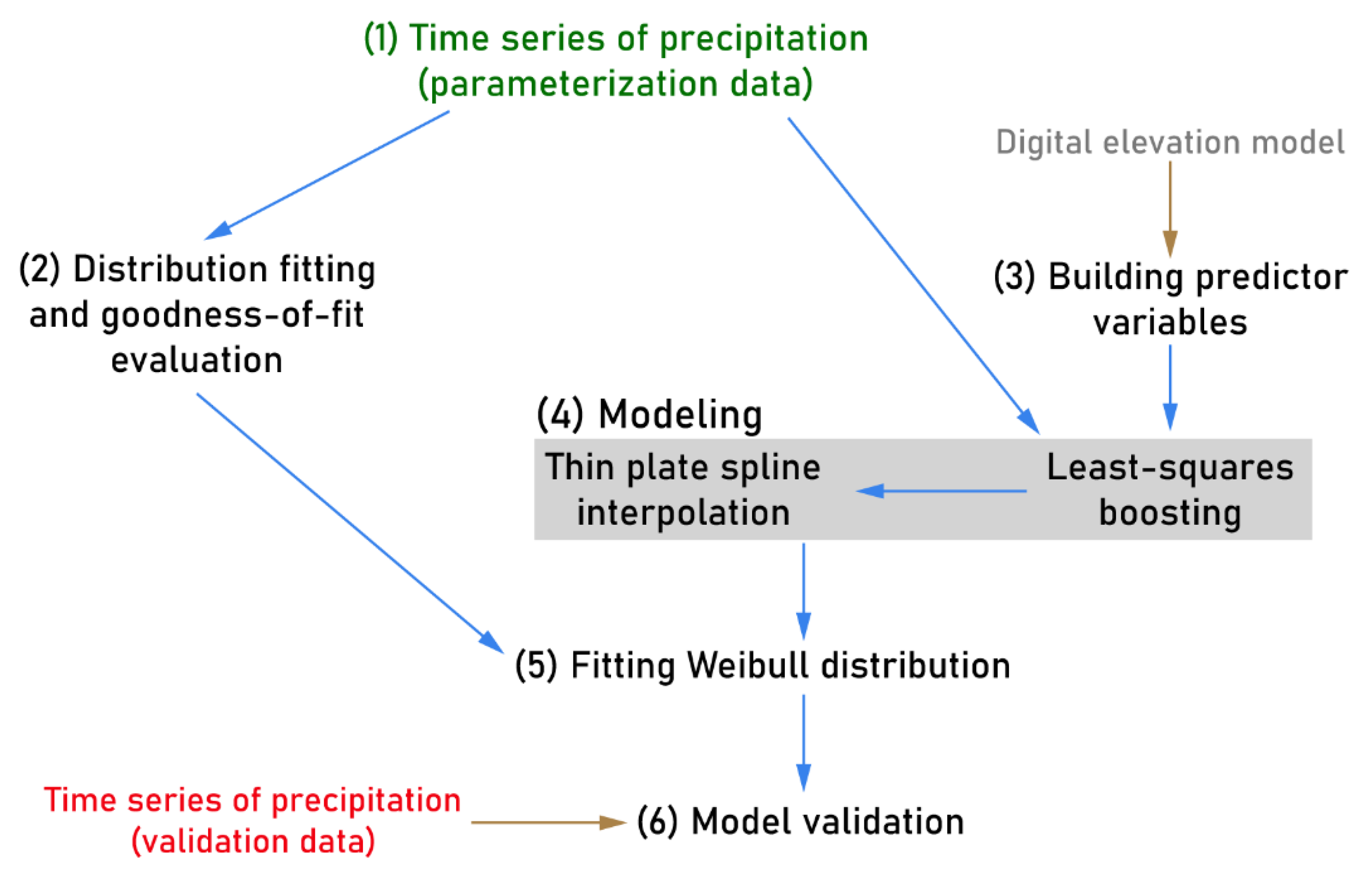
2.1. Overview

The development of GePrA was composed of the following main steps (Figure 1): (1) Obtaining daily precipitation data (parametrization data) provided by the German Meteorological Service for the period 1981–2018; (2) fitting of 18 theoretical distributions to the precipitation time series and evaluation of their goodness-of-fit; (3) building of predictor variables representing the local orography based on a digital elevation model; (4) high spatial resolution modeling (25 m × 25 m) of the percentiles by a least-squares boosting approach and thin plate spline interpolation; (5) fitting of Weibull distributions, which provide the best fits, to the modeled precipitation percentiles; and (6) model validation by independent precipitation data (validation data).

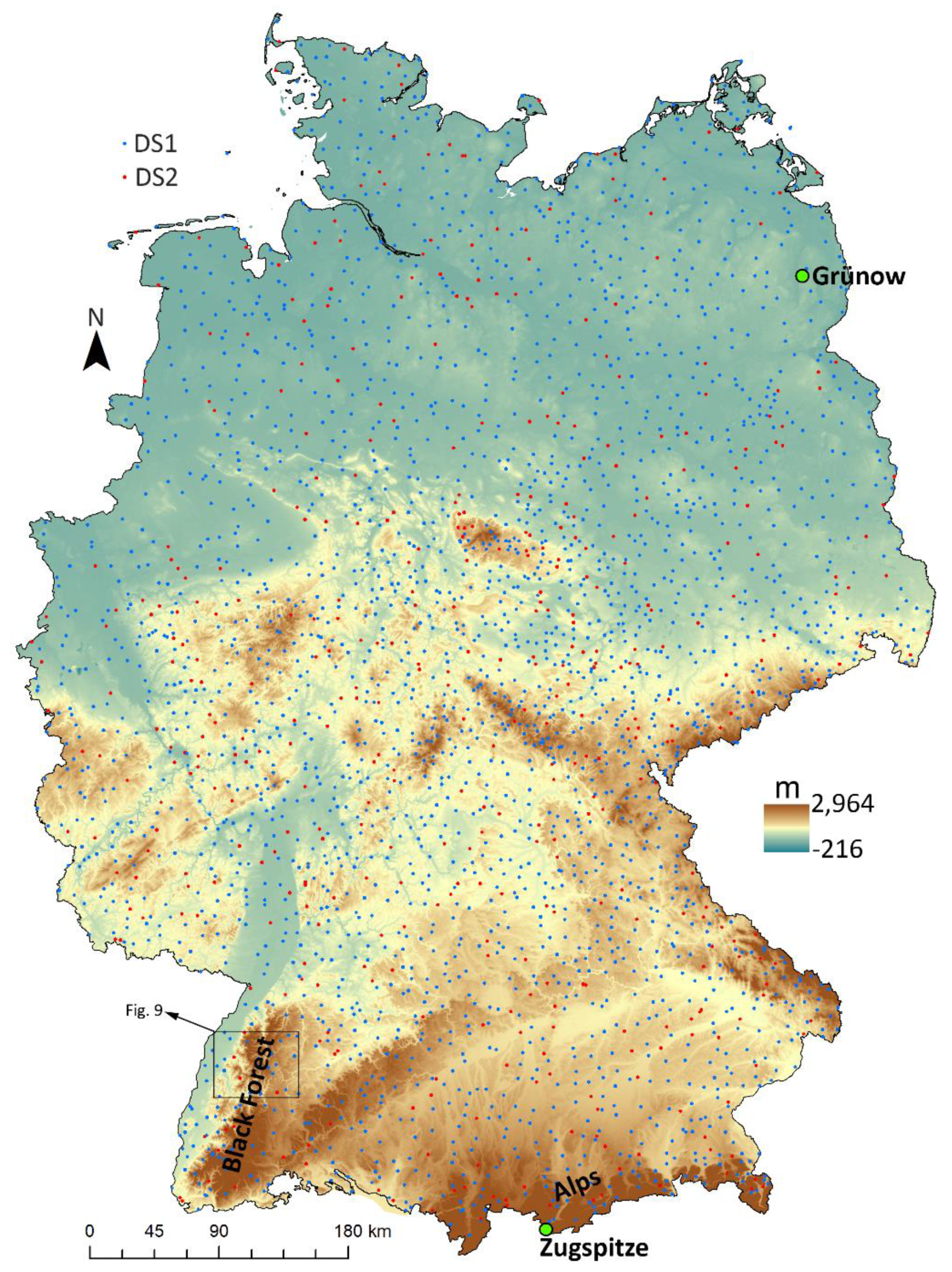
2.2. Study Area and Precipitation Data

Germany has a size of about 357,000 km². The country consists of the four large natural areas: The North German Plain, Central German Plain, Alpine Foothills, and Alps in southern Germany [20]. Its topography is complex and ε ranges from below 0 m to nearly 3000 m (Figure 2). Besides the high mountain range of the Alps, there are numerous low mountain ranges (500 m < ε < 1500 m). The highest and largest contiguous low mountain range is the Black Forest in the southwest.

The study was based on daily precipitation (RR) measurements of the period 1981–2018 available from the German Meteorological Service climate data center [21]. Depending on the availability of RR data (DA), RR time series were assigned to either the parameterization dataset (DS1) or to the validation dataset (DS2). DS1 contained 2357 RR time series with DA > 50%. DS2 included 425 RR time series with DA being in the range of 40.0% to 49.9%. All other and less complete time series were not considered for further analysis.

2.3. Distribution Fitting

The selection of suitable theoretical distributions is of great importance for the accurate description of the statistical properties of precipitation time series. Thus, different statistical distributions used in previous studies [22,23] were tested. From these distributions, those with less than four parameters were selected (

Table 1. Theoretical distributions fitted to daily precipitation (RR) including their parameters [25].

Distribution	Abbreviation	Parameters
Beta	Be	shape, shape
Birnbaum-Saunders	BS	shape, scale
Burr	Bu	shape, shape, scale
Epsilon Skew Normal	ESN	scale, location, skewness
Extreme Value	EV	location, scale
Gamma	Gam	shape, scale
Generalized Extreme Value	GEV	shape, scale, location
Generalized Pareto	GP	shape, scale, location
Inverse Gaussian	IG	scale, shape
Logistic	L	mean, scale
Log-logistic	LL	mean, scale (of logarithmic values)
Lognormal	LN	mean, standard deviation (of logarithmic values)
Nakagami	Na	shape, scale
Normal	N	mean, standard deviation
Poisson	P	mean
Rician	R	non-centrality, scale
t-Location Scale	tLS	location, scale, shape
Weibull	Wei	shape, scale

). The distributions were fitted to monthly empirical cumulative distribution functions (ecdf) of RR included in DS1 by applying the maximum likelihood method. As there is often a very high proportion of RR = 0 mm, the distributions were only fitted to RR > 0 mm. The goodness-of-fit (GoF) of each theoretical distribution was assessed by the Kolmogorov-Smirnov statistic (KS), the coefficient of determination related to the cumulative probability ($R_{PP}^2$), and the coefficient of determination related to the quantiles ($R_{QQ}^2$) [24].

The distribution fitting was made using Mathworks’ Matlab^® Software Statistics and Machine Learning Toolbox (Release 2019a; The MathWorks Inc., Natick, MA, USA).

2.4. Predictor Variables

The orographic features (

Table 2. Orographic features used as predictor variables (PV) for modeling daily precipitation (RR).

Symbol	Name	Sector (°)	Distance (m)	Data Source
lon	longitude	-	-	-
lat	latitude	-	-	-
ε	elevation	-	-	EU-DEM v.1
η1000	relative elevation	1–360	1000	EU-DEM v.1
η3000	relative elevation	1–360	3000	EU-DEM v.1
η5000	relative elevation	1–360	5000	EU-DEM v.1
η7500	relative elevation	1–360	7500	EU-DEM v.1
ηn	relative elevation	337.5–22.4	3000	EU-DEM v.1
ηne	relative elevation	22.5–67.4	3000	EU-DEM v.1
ηe	relative elevation	67.5–112.4	3000	EU-DEM v.1
ηse	relative elevation	112.5–157.4	3000	EU-DEM v.1
ηs	relative elevation	157.5–202.4	3000	EU-DEM v.1
ηsw	relative elevation	202.5–247.4	3000	EU-DEM v.1
ηw	relative elevation	247.5–292.4	3000	EU-DEM v.1
ηnw	relative elevation	292.5–337.4	3000	EU-DEM v.1
σn	sheltering	337.5–22.4	1000	EU-DEM v.1
σne	sheltering	22.5–67.4	1000	EU-DEM v.1
σe	sheltering	67.5–112.4	1000	EU-DEM v.1
σse	sheltering	112.5–157.4	1000	EU-DEM v.1
σs	sheltering	157.5–202.4	1000	EU-DEM v.1
σsw	sheltering	202.5–247.4	1000	EU-DEM v.1
σw	sheltering	247.5–292.4	1000	EU-DEM v.1
σnw	sheltering	292.5–337.4	1000	EU-DEM v.1
σsum	sheltering	1–360	1000	EU-DEM v.1

) were represented by 22 predictor variables (PV) derived from the digital elevation model EU-DEM v.1 at a 25 m × 25 m spatial resolution [26]. The relative elevation (η) was developed by subtracting the mean elevation of an outer circle of each grid cell from the grid cell-specific ε value [27]. Four η variants with outer-circle radii of 1000 m (η₁₀₀₀), 3000 m (η₃₀₀₀), 5000 m (η₅₀₀₀), and 7500 m (η₇₅₀₀) were built. For the eight main compass directions, η was modeled with a 3000 m radius. Furthermore, the orographic sheltering (σ) was quantified. It was derived by calculating the angles between grid cell-specific elevation and the visible horizon up to a distance of 1000 m [27].

2.5. LS-Boost Modeling (LSBoost) and Thin Plate Spline Interpolation (TPS)

The RR percentiles ($R{R}_p$), being p = {1, 5, 10, 15, 20, 25, 30, 35, 40, 45, 50, 55, 60, 65, 70, 75, 80, 85, 90, 95, 99}, were modeled in a two-step procedure: (1) A least-squares boosting (LSBoost) algorithm was trained for RR included in DS1 using PV; and (2) the remaining DS1 residuals were further reduced by applying a thin plate spline interpolation (TPS). The modeling of RR return times associated with greater p > 99 (corresponding to a return period of 100 days) was omitted because they would exceed the limitations with which a reliable model can be developed given the length of the available dataset and would require an extreme value analysis [28].

The LSBoost model is a sequence of regression trees (B), i.e., decision trees with binary splits for regression [29,30,31]. The LSBoost model strives to reduce the mean squared error (MSE) between $R{R}_p$ and the aggregated $R{R}_p$ prediction (${\widehat{RR}}_p$) of B. Starting with the median of $R{R}_p$ (${\widetilde{RR}}_p$) of all DS1 stations, the regression trees B₁, …, B_m were combined in a weighted manner [29,30,31] to minimize MSE. Mathematically, the LSBoost algorithm is described as:

$${\widehat{RR}}_p\left(PV\right)={\widetilde{RR}}_p\left(PV\right)+v{{\displaystyle \sum }}_{m=1}^M{p}_m{B}_m\left(PV\right),$$

(1)

where p_m is the weight for model m, M is the total number of regression trees, and 0 < v ≤ 1 is the learning rate.

More than 5000 predictor variable combinations (PVC) were tested for their predictive power. Evaluation of the five-fold cross-validated R² revealed the most powerful PVC associated with DS1. The applied LSBoost algorithm was available from the Matlab^® Software Statistics and Machine Learning Toolbox (Release 2019a; The Math Works Inc., Natick, MA, USA).

The predictors lon and lat, which describe the geographic location of a measurement station, were used as input for TPS [32]. The applied TPS algorithm was implemented in the Matlab^® Software Curve Fitting Toolbox (Release 2019a; The Math Works Inc., Natick, MA, USA).

Wet days were defined when ${\widehat{RR}}_p$ > 0 (PR_wet). Wei, which was found to provide the best fitting accuracy, was fitted to ${\widehat{RR}}_p$ on wet days applying the least-squares estimation method [33] The probability density function of Wei (f(RR)) is defined as [33]:

$$f\left(RR;\alpha ,k\right)=\frac{k}{\alpha }{\left(\frac{RR}{\alpha }\right)}^{k-1}exp\left[-{\left(\frac{RR}{\alpha }\right)}^k\right],$$

(2)

where k is the shape parameter and $\alpha$ is the scale parameter. From PR_wet and f(RR), the mean monthly precipitation sum (${\overline{RR}}_{sum}$) was then calculated:

$${\overline{RR}}_{sum}=\alpha \Gamma \left(1+\frac{1}{k}\right)·nm·R{R}_{wet},$$

(3)

where $\Gamma$ is the Gamma function and nm is the number of days per month.

After completion of RR_p modeling and distribution fitting, the model was validated for ${\overline{RR}}_{sum}$ calculation using DS2. The model quality was assessed by applying R², mean absolute error (MAE), and mean error (ME).

2.6. Inter-Area Variability

The variability of $R{R}_{sum}$ within the study area was quantified by the interarea variability (IAV) according to:

$$IAV=\frac{S}{⟨{\overline{RR}}_{sum}\rangle },$$

(4)

where $S$ is the standard deviation of ${\overline{RR}}_{sum}$, and $⟨{\overline{RR}}_{sum}\rangle$ is the mean of ${\overline{RR}}_{sum}$ in the study area.

3. Results and Discussion

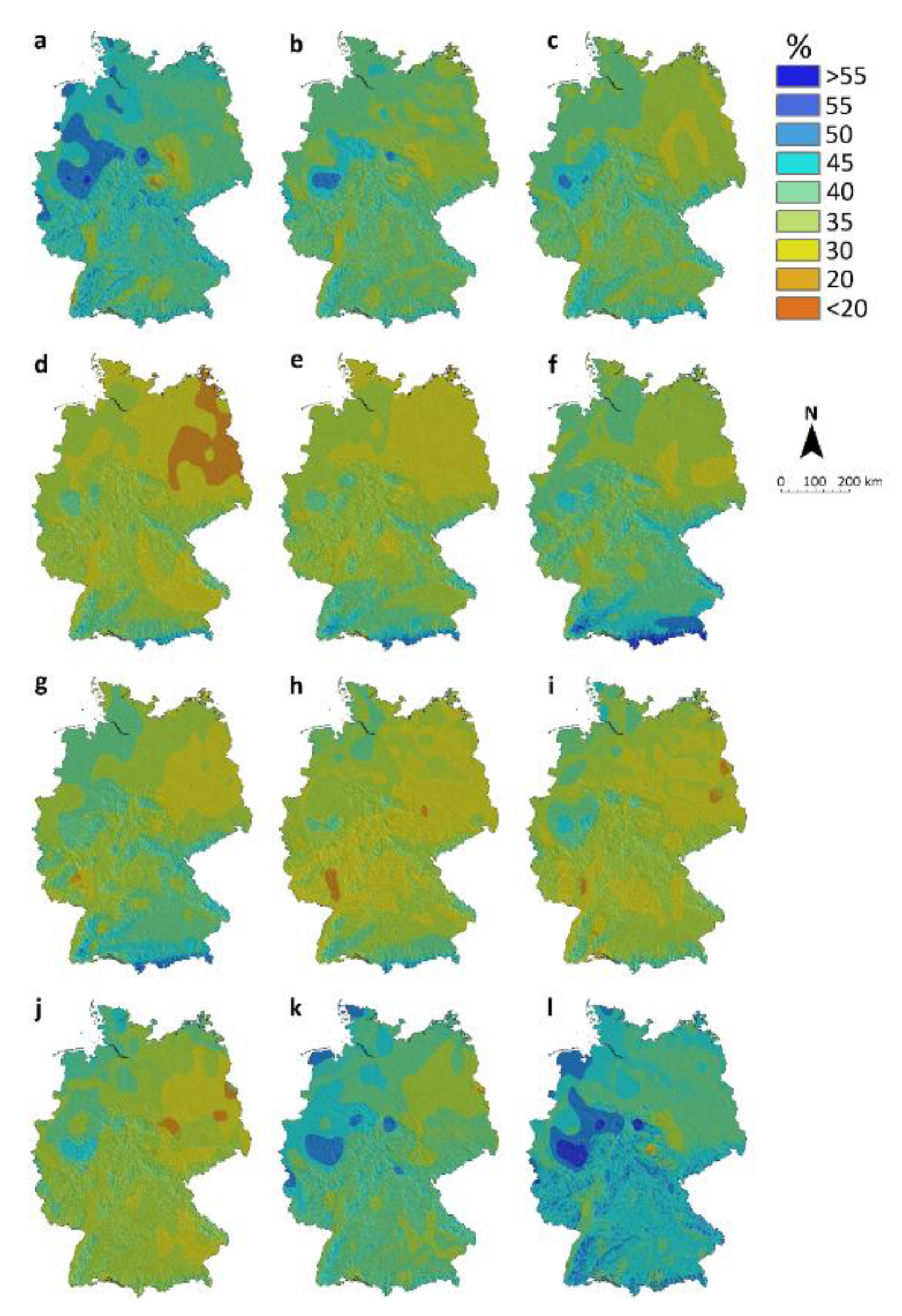
3.1. Proportion of Wet Days (PR_wet)

The monthly PR_wet is displayed in Figure 3. The mean PR_wet in the study area $(⟨P{R}_{wet}\rangle )$was lowest ($⟨P{R}_{wet}\rangle$= 33%) in April (Figure 3d) and highest ($⟨P{R}_{wet}\rangle$= 44%) in December (Figure 3l). In addition to the temporal PR_wet variability, there was also a strongly pronounced spatial PR_wet pattern. In January (Figure 3a), February (Figure 3b), March (Figure 3c), October (Figure 3j), November (Figure 3k), and December, the highest PR_wet values occurred in the west (PR_wet > 50%). The precipitation in these months was mainly caused by precipitation fronts from the west. In contrast, in May (Figure 3e), June (Figure 3f), and July (Figure 3g), the highest PR_wet values occurred in the Alps (PR_wet > 50%). During summer, the high PR_wet values in this area were caused by a high frequency of convective precipitation events [34].

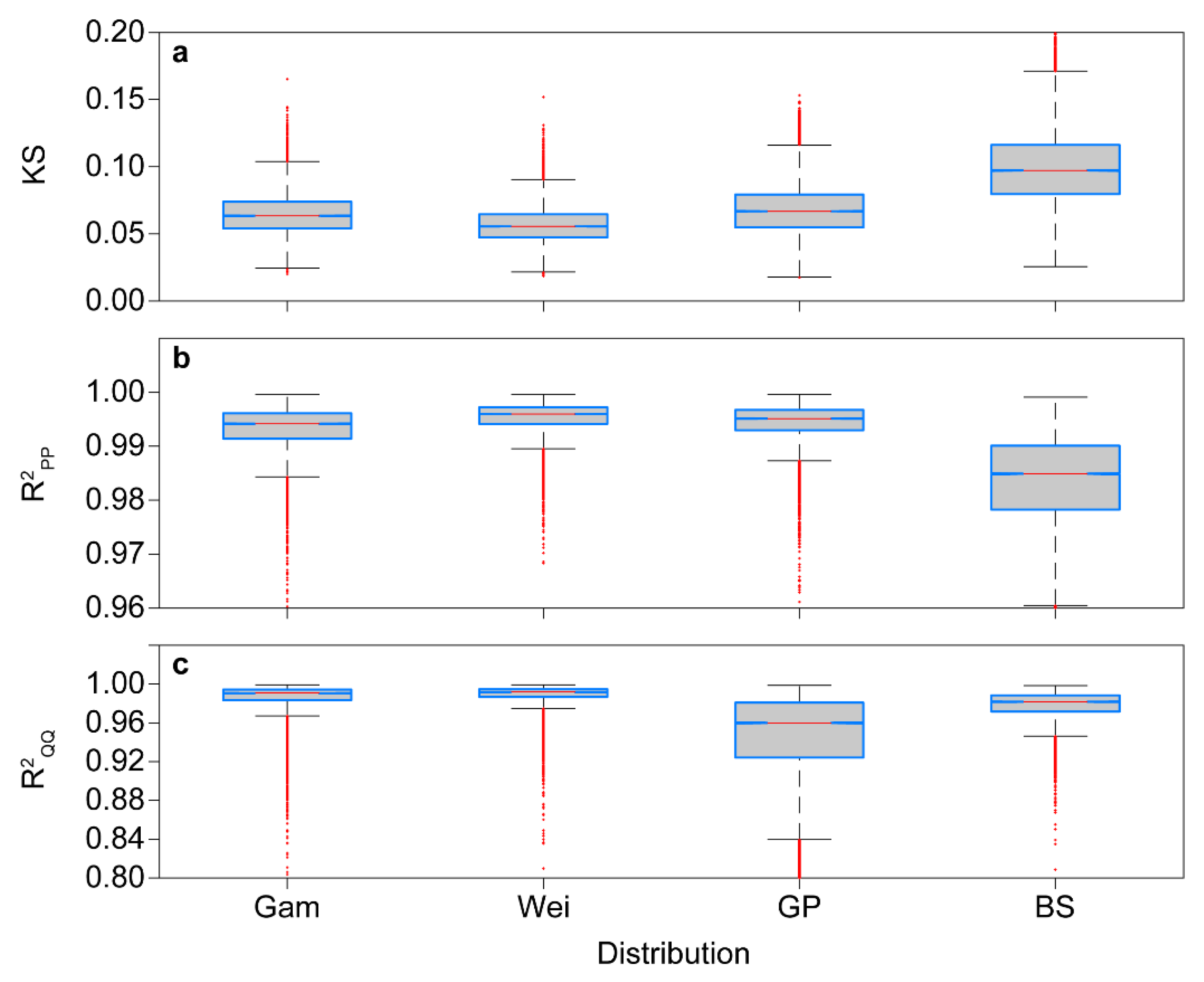
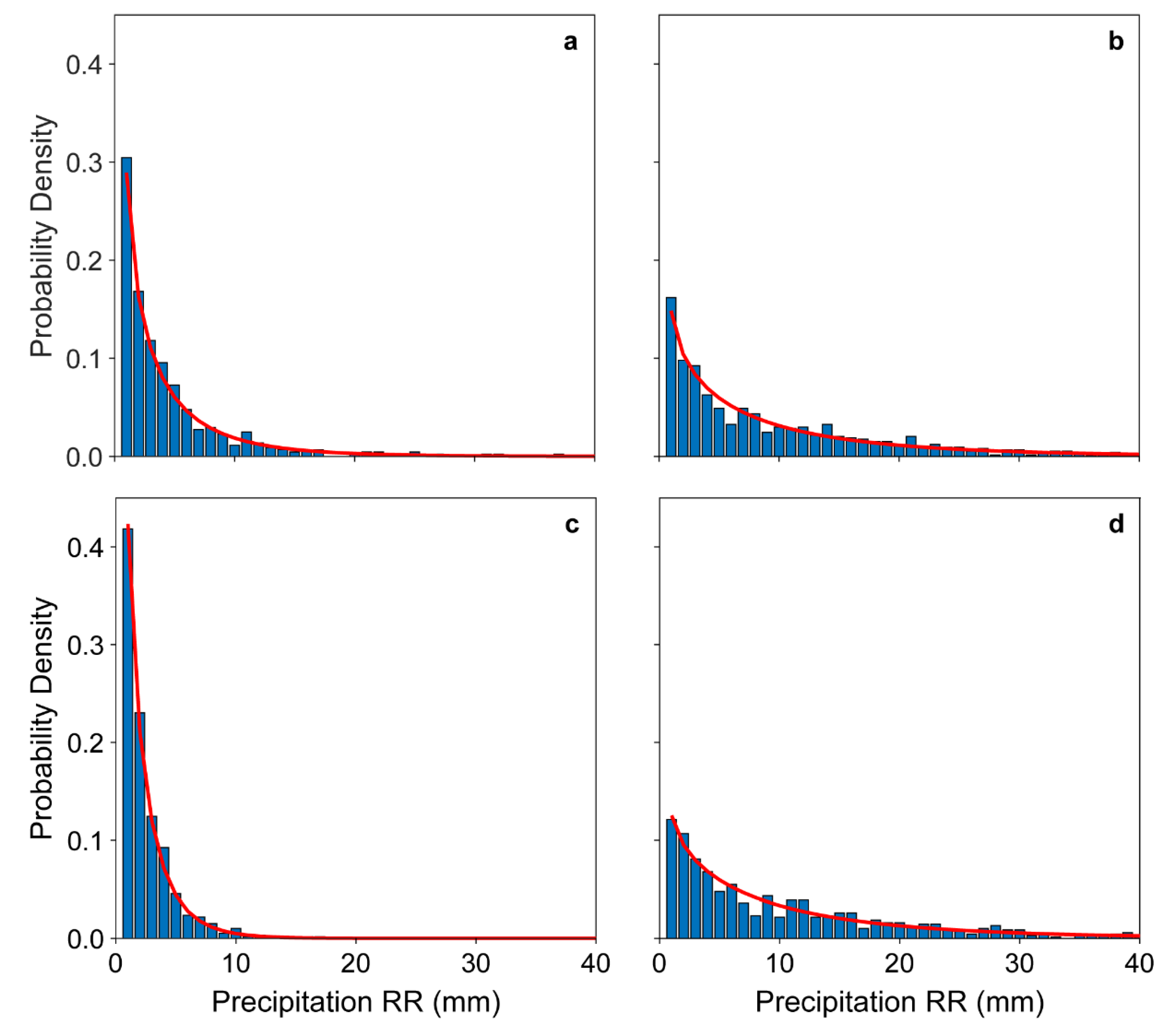
3.2. Distribution Fitting

Results from the GoF evaluation are summarized in Figure 4 for all months. Out of the 18 candidate theoretical distributions, Gam, Wei, GP, and BS could be fitted to all empirical distributions in all months yielding accurate fits. All other theoretical distributions could either not be fitted to all RR time series or their GoF was low.

According to KS, Wei was the best fitting theoretical distribution (Figure 4a). The median KS of Wei was 0.055, the first quartile was 0.047, and the third quartile was equal to 0.065. For Gam, GP, and BS, median KS varied between 0.063 and 0.097. Similar results were found for $R_{PP}^2$ (Figure 4b). The median $R_{PP}^2$ for Wei was 0.996 and was thus close to a perfect match between the theoretical and empirical distribution. For Gam and GP, the median $R_{PP}^2$ was only slightly worse (0.994 resp. 0.995). The outliers obtained by Wei were not lower than 0.97, indicating a reliable fitting accuracy. The third calculated GoF confirms the capability of Wei to mimic f(RR) (Figure 4c). Its median $R_{QQ}^2$ was 0.992. A similarly high GoF could only be achieved by Gam (median of $R_{QQ}^2$ = 0.991). Based on the GoF evaluation, Wei was assumed to be generally able to reproduce f(RR) on wet days.

All of the RR probability density functions had similar shapes. In general, (1) the lowest RR values have the highest probability density, and (2) the probability density decreases with increasing RR. As an example of the coincidence of the empirical probability density and Wei, the results for two different locations in summer (Jun–Aug, JJA) and winter (Dec–Feb, DJF) are presented in Figure 5.

For the city of Grünow, which is located in the northeast of the study area, f (RR) is shown for August (Figure 5a). From this, it can be inferred that Grünow was very dry during summer. The frequency of RR < 1.5 mm was highest (0.305). During summer, RR rarely exceeded 20 mm (0.027). The Wei function reproduced the shape of the histograms very accurately.

The second example shows f(RR) in August for Germany’s highest peak, the Zugspitze (Figure 5b). Overall, the probability density of high RR was much higher compared to Grünow. For instance, f (RR = 0 mm) was 0.148 and f (RR > 20 mm) was 0.125.

In December, the probability density of low RR values increased in Grünow (Figure 5c), with f(RR) = 1 mm being 0.42. The exceedance probability of 10.4 mm was only 0.01, indicating that high RR values were extremely rare.

On the Zugspitze, the differences between f(RR) in August and f(RR) in December were marginal (Figure 5d). The probability density of f (RR) > 10.4 mm was even higher (0.35) in December. The examples show a broad spectrum of different RR regimes. Nevertheless, the fitting of Wei was always very close to the empirical histogram.

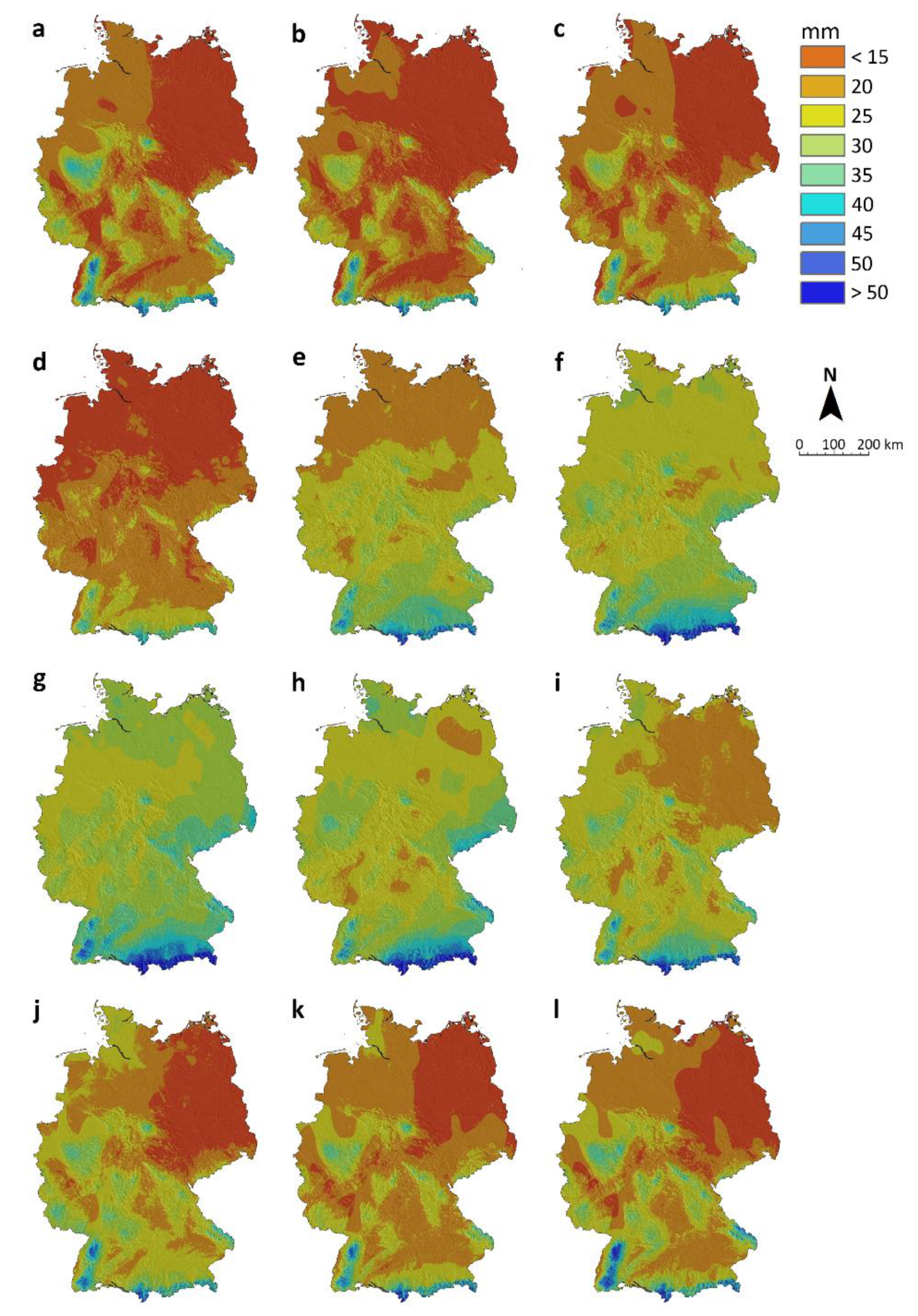
3.3. Heavy Precipitation

As an example of heavy precipitation, ${\widehat{RR}}_{99}$ is shown in Figure 6. It corresponds to a return period of 100 days. Similar to PR_wet, summer months were more precipitous than all other months. In July, the highest ${\widehat{RR}}_{99}$ values generally occurred. The mean ${\widehat{RR}}_{99}$ in the study area ($⟨{\widehat{RR}}_{99}\rangle$) in July was equal to 28.3 mm (Figure 6g). In contrast, $⟨{\widehat{RR}}_{99}\rangle$in February was only 16.0 mm (Figure 6b). In May and September, $⟨{\widehat{RR}}_{99}\rangle$corresponded to 23.3 mm, whereas in March, April, and November, $⟨{\widehat{RR}}_{99}\rangle$ < 20 mm.

The ${\widehat{RR}}_{99}$ gradient in DJF is west-east oriented whereas in the summer months it is more northwest-southeast oriented. An important reason for this could be that heavy precipitation in winter is mainly stratiform [35] and predominantly from western directions. In summer, precipitation is predominantly convective. However, there are also regions in DJF were ${\widehat{RR}}_{99}$ is very high. In the low mountain ranges, especially on their west-east oriented slopes, ${\widehat{RR}}_{99}$ is often higher in winter than in the summer. In December, ${\widehat{RR}}_{99}$ frequently exceeds 50 mm in the Black Forest and near the Alps (Figure 6l). By comparison, in eastern Germany, ${\widehat{RR}}_{99}$ is clearly lower at less than 15 mm. Overall, the ${\widehat{RR}}_{99}$ variability is greater in winter than in summer. This indicates that the small-scale properties of the orography determine the heavy precipitation pattern in winter.

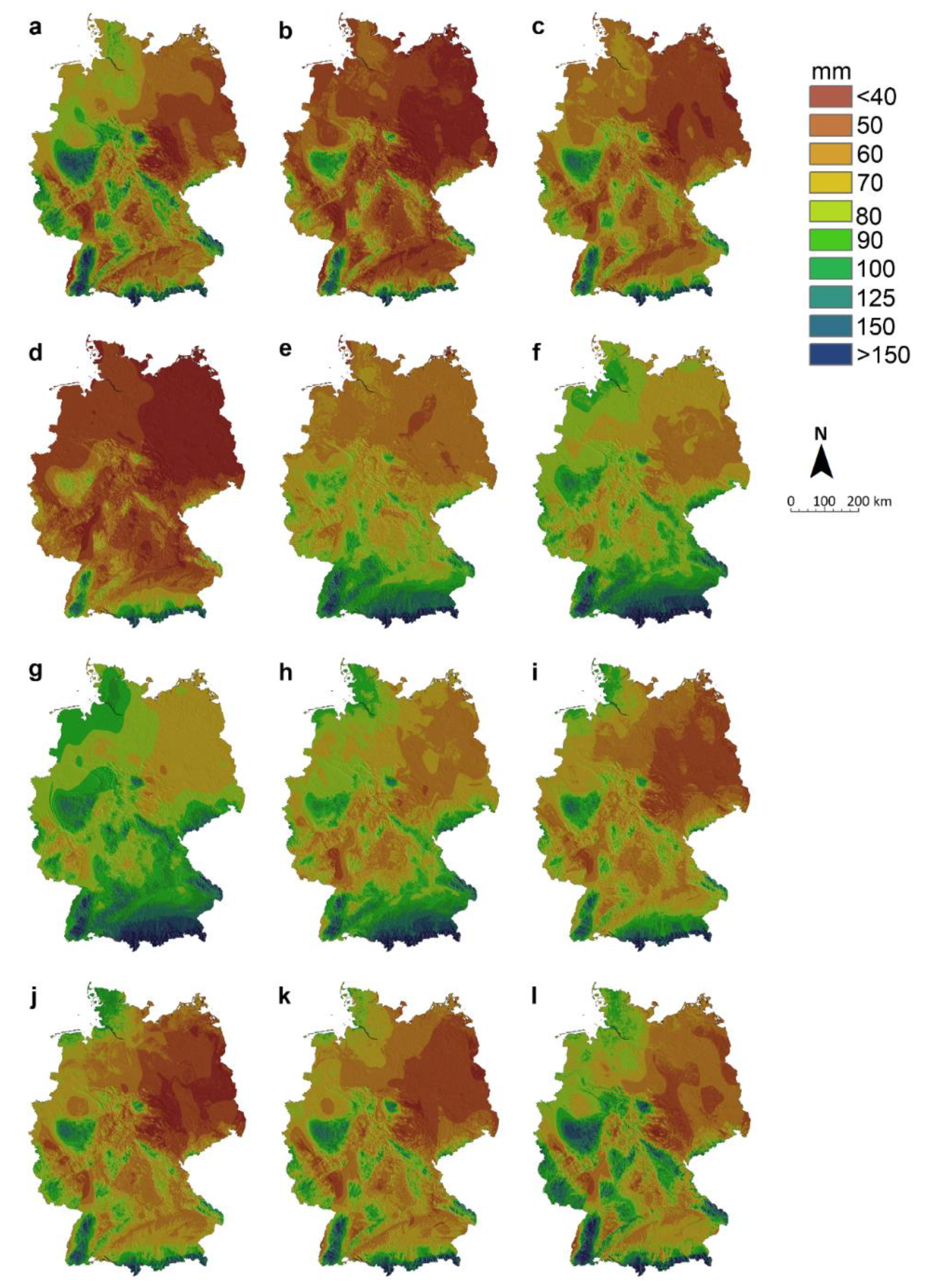
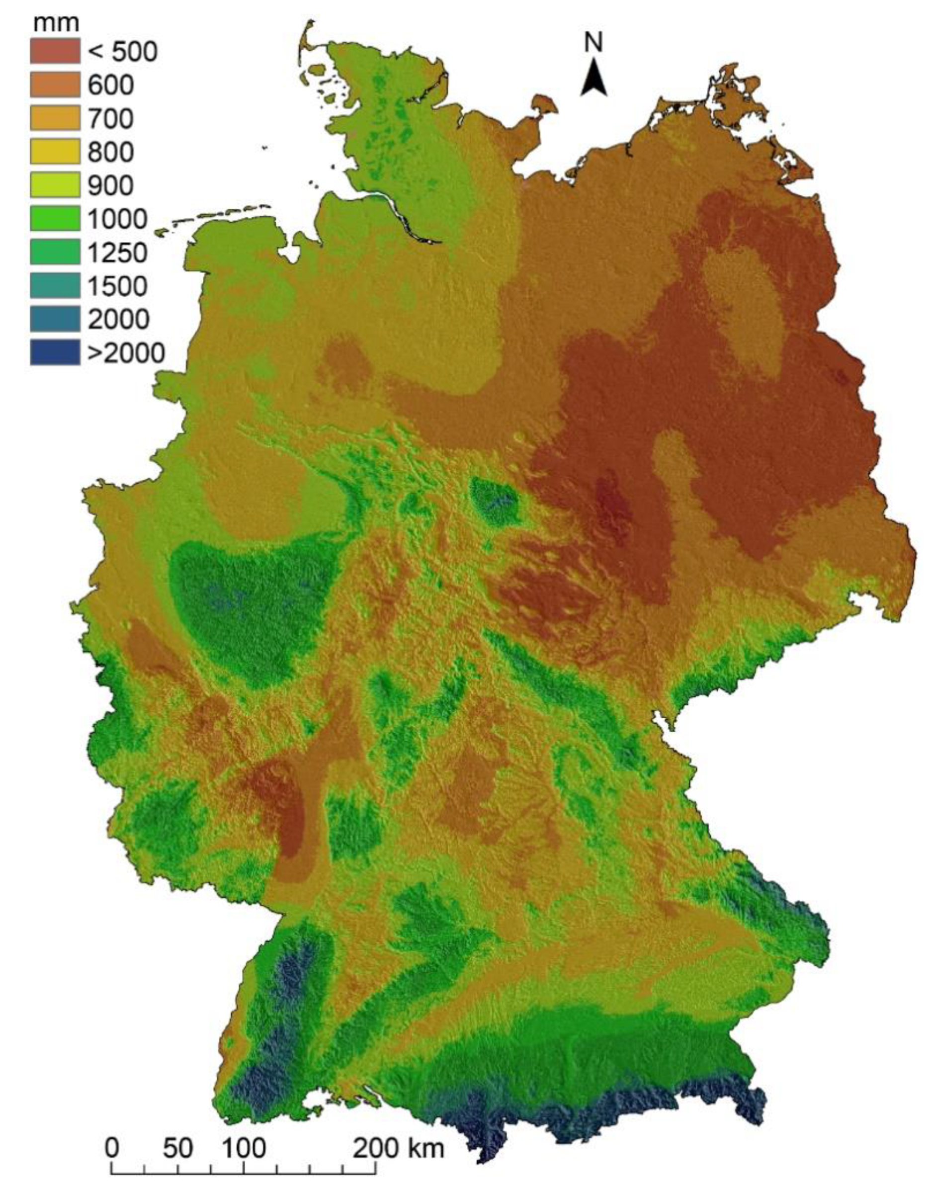
3.4. Monthly and Annual Precipitation Sums

In Figure 7, ${\overline{RR}}_{sum}$ is presented. The large-scale spatial pattern shows similarities to the ${\widehat{RR}}_{99}$ pattern. In January (Figure 7a) and December (Figure 7l), ${\overline{RR}}_{sum}$ was highest on the west–east oriented slopes of the western low mountain ranges, where it often exceeded 150 mm. In contrast, in the eastern parts of Germany, ${\overline{RR}}_{sum}$was frequently below 50 mm.

In the study area, ${\overline{RR}}_{sum}$ was highest ($⟨{\overline{RR}}_{sum}\rangle$ = 84 mm) in July (Figure 7g) and lowest ($⟨{\overline{RR}}_{sum}\rangle$ = 49 mm) in April (Figure 7d). The annual ${\overline{RR}}_{sum}$ cycle in the study area had two maxima: One in July and a second in December. At the regional scale, the annual ${\overline{RR}}_{sum}$ cycle may differ from $⟨{\overline{RR}}_{sum}\rangle$. For instance, in the vicinity of the Alps, ${\overline{RR}}_{sum}$ was often more than twice as high in JJA compared to DJF. In contrast, in some areas of the western low mountain ranges, the maximum ${\overline{RR}}_{sum}$ was modeled in December.

The interarea variability of ${\overline{RR}}_{sum}$ in the study area was highest (IAV = 3.6) in September (Figure 7i), October (Figure 7j), and November (Figure 7k). This indicates that both the large-scale and orographic influence on ${\overline{RR}}_{sum}$ in these months were strong. In contrast, ${\overline{RR}}_{sum}$ was more evenly distributed (IAV = 2.9) in April (Figure 7d).

The mean annual precipitation sum (${\overline{RR}}_{sum,yr}$) is displayed in Figure 8. In the study area, it corresponded to $⟨{\overline{RR}}_{sum,yr}\rangle$ = 790 mm and tended to increase toward the south and decrease toward the east. In most of the low mountain ranges, ${\overline{RR}}_{sum,yr}$ usually exceeded 1000 mm. In the southern low mountain ranges and close to the Alps, ${\overline{RR}}_{sum,yr}$ often exceeded 1500 mm. At individual sites, ${\overline{RR}}_{sum,yr}$ may even be higher than 2000 mm.

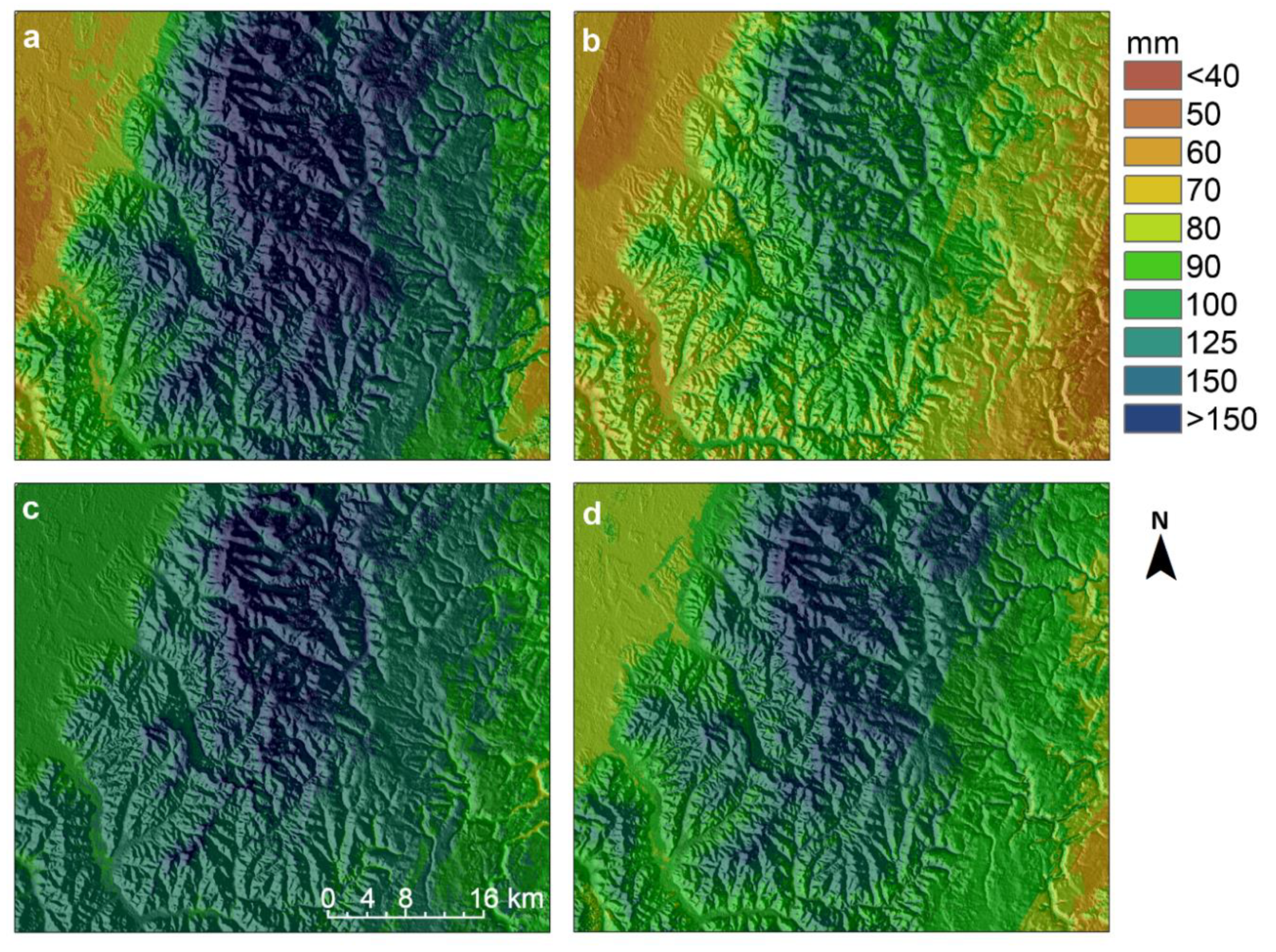
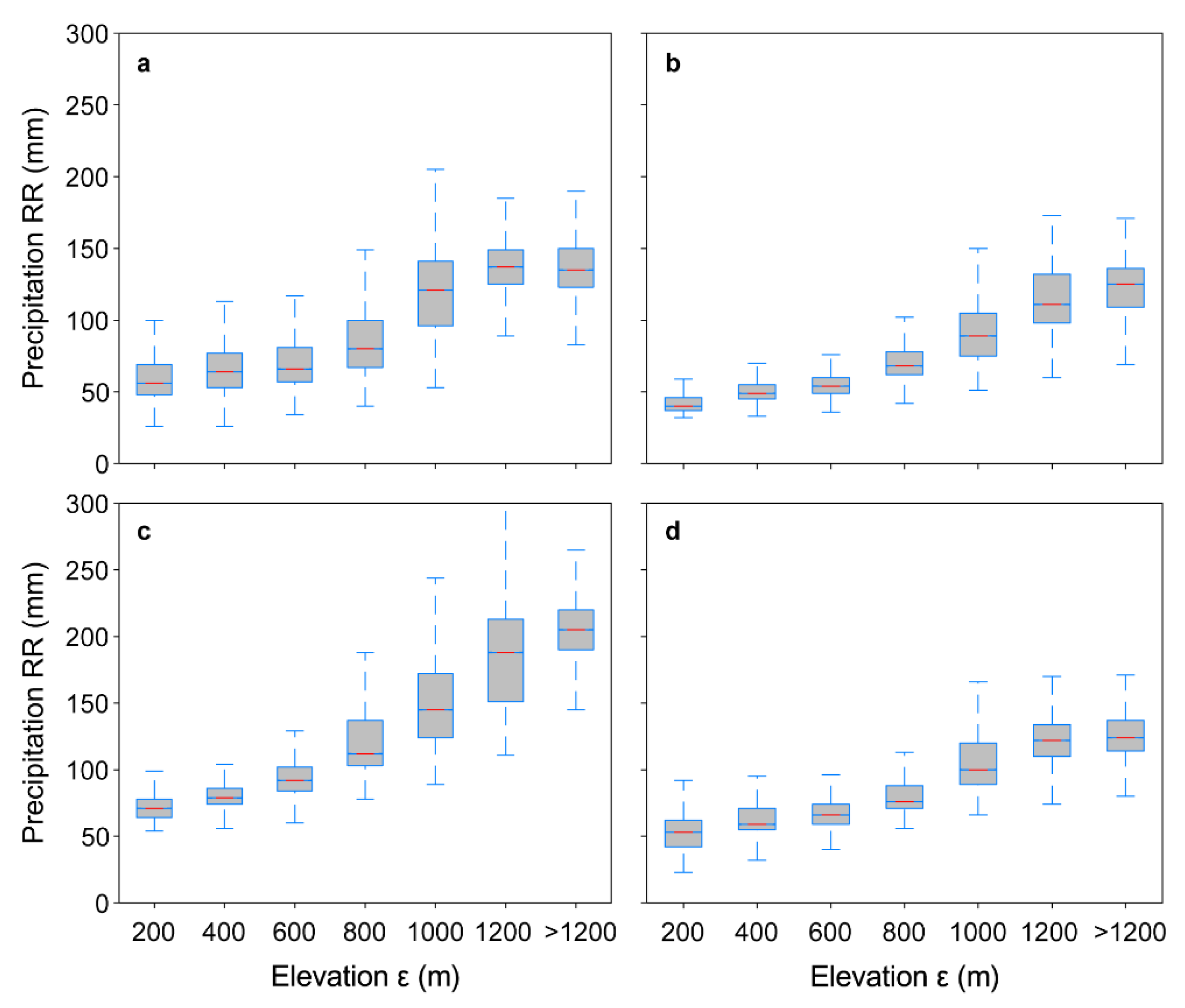
3.5. Orographic Influence on Precipitation Sums

The small-scale variability of precipitation over the course of the year is highlighted for the low mountain range of the Black Forest in Figure 9. In January, ${\overline{RR}}_{sum}$ varied from ≈ 50 mm to almost 200 mm over a distance of less than 30 km (Figure 9a). The highest ${\overline{RR}}_{sum}$ values occurred on the high mountain slopes exposed to the west. The lowest ${\overline{RR}}_{sum}$ values can be found in the lowest regions of the map extract. The spatial pattern of ${\overline{RR}}_{sum}$ remained similar in April (Figure 9b). However, the ${\overline{RR}}_{sum}$ variability decreased compared to January. This was mainly due to the fact that ${\overline{RR}}_{sum}$ was lower at high elevations compared to January. In July, ${\overline{RR}}_{sum}$ increased in the entire study area (Figure 9c). In almost the entire map extract, ${\overline{RR}}_{sum}$ > 90 mm. In the high elevation regions, ${\overline{RR}}_{sum}$ was slightly lower compared to January. In October, ${\overline{RR}}_{sum}$ tendencies remained similar to the other months (Figure 9d). ${\overline{RR}}_{sum}$ ranged from 75 mm to 160 mm. From the presented figure, it can be deduced that (1) elevation had a significant influence on ${\overline{RR}}_{sum}$ and (2) its effect on ${\overline{RR}}_{sum}$ varied over the course of the year.

To quantify the dependency of ${\overline{RR}}_{sum}$ on ε, boxplots of ${\overline{RR}}_{sum}$ as a function of ε are shown in Figure 10. In January, ${\overline{RR}}_{sum}$ increased only slightly, with increasing ε until 600 m (Figure 10a). Above 800 m, ${\overline{RR}}_{sum}$ rapidly increased. At ε > 1200 m, ${\overline{RR}}_{sum}$ remained quasi-constant. The variability of ${\overline{RR}}_{sum}$ was greatest at ε ≈ 1200 m. A possible reason for this is that the orographic features (e.g., orientation, inclination) are very diverse in this elevation range.

In April, the interquartile range of ${\overline{RR}}_{sum}$ was lower, especially at low ε (Figure 10b). In July, the rate of ${\overline{RR}}_{sum}$ change as a function of ε was greatest (Figure 10c). The median ${\overline{RR}}_{sum}$ increased from 71 mm at ε = 200 m to 205 mm at ε > 1200 m. In addition, ${\overline{RR}}_{sum}$ variability also increased. Both the general ${\overline{RR}}_{sum}$ level and the variability of ${\overline{RR}}_{sum}$ decreased in October (Figure 10d). The median of ${\overline{RR}}_{sum}$ increased from 53 mm at ε = 200 m to 124 mm at ε > 1200 m.

3.6. Model Validation

Results from model validation are summarized in

Table 3. Model validation evaluated by the coefficient of determination (R²), the mean absolute error (MAE), and mean error (ME) calculated for the mean monthly precipitation sum (${\overline{RR}}_{sum}$) and the mean annual precipitation sum (${\overline{RR}}_{sum,yr}$).

Month	R2	MAE (mm)	ME (mm)
January	0.78	9	1
February	0.70	8	1
March	0.76	9	1
April	0.75	7	1
May	0.83	8	0
June	0.87	8	0
July	0.87	9	0
August	0.85	8	0
September	0.80	8	0
October	0.79	8	1
November	0.75	8	0
December	0.78	9	0
Year	0.91	9	1

. From this summary, it can be seen that the R² ranged from 0.70 in February to 0.87 in June and July. In 11 months, the R² exceeded 0.75. From May to September, R² > 0.80, which indicates that the accuracy of the model used to simulate ${\overline{RR}}_{sum}$ was higher in summer than in winter. The ${\overline{RR}}_{sum,yr}$ model had the highest accuracy (R² = 0.91). Further, MAE indicates that the accuracy of the models was very good (below 10 mm in all months). For ${\overline{RR}}_{sum,yr}$, MAE = 9 mm. ME indicates that there was no bias in the models, because it was either 0 mm or 1 mm in all months and on the annual scale.

4. Conclusions

In this study, daily precipitation was modeled monthly at a very high resolution in Germany. It was demonstrated that the annual precipitation cycle depends on regions and orographic properties such as elevation, relative elevation, and topographic sheltering. The high resolution provided the foundation for a very detailed detection of local precipitation regimes. According to the rigorous goodness-of-fit evaluation using a parametrization dataset and a validation dataset, the accuracy of the models built was good. The coefficient of determination reached values up to 0.91, which was achieved by evaluating the results from modeling the mean annual precipitation sum.

One important feature of GePrA is that it is not limited to the mapping of large-scale precipitation patterns. It can also be used to quantify the effects of the local orography on monthly and annual precipitation. Moreover, GePrA does not only reproduce the monthly and annual precipitation sums, but also the entire monthly precipitation distributions. The two parameters of the Weibull distribution used to fit the empirical precipitation distributions and the share of wet days are available monthly for all grid cells in the study area. Using the monthly Weibull parameters and the share of wet days, it was possible to calculate any percentile and the monthly precipitation sum.

Although the developed models reflect the monthly distribution of precipitation very well, the results and the approach are not without limitations. GePrA does not indicate precipitation intensity on sub-monthly scales. The statistical approach of GePra does not allow the mapping of daily precipitation conditions. No direct relationship can be established between individual synoptic conditions and the simulated precipitation sums. Furthermore, it is not possible to map extreme heavy precipitation events with return periods exceeding 100 days. It is possible to transfer the proposed approach to the analysis of extreme precipitation events, but that would require longer time series than those used in this study.

References

1. Iqbal, M.F.; Athar, H. Validation of satellite based precipitation over diverse topography of Pakistan. Atmos. Res. 2018, 201, 247–260. [Google Scholar] [CrossRef]
2. Zuo, J.; Xu, J.; Chen, Y.; Wang, C. Downscaling Precipitation in the Data-Scarce Inland River Basin of Northwest China Based on Earth System Data Products. Atmosphere 2019, 10, 613. [Google Scholar] [CrossRef]
3. Yang, T.; Shao, Q.; Hao, Z.C.; Chen, X.; Zhang, Z.; Xu, C.Y.; Sun, L. Regional frequency analysis and spatio-temporal pattern characterization of rainfall extremes in the Pearl River Basin, China. J. Hydrol. 2010, 380, 386–405. [Google Scholar] [CrossRef]
4. Putniković, S.; Tošić, I. Relationship between atmospheric circulation weather types and seasonal precipitation in Serbia. Meteorol. Atmos. Phys. 2018, 130, 393–403. [Google Scholar] [CrossRef]
5. Hiebl, J.; Frei, C. Daily precipitation grids for Austria since 1961—Development and evaluation of a spatial dataset for hydroclimatic monitoring and modelling. Theor. Appl. Climatol. 2018, 132, 327–345. [Google Scholar] [CrossRef]
6. Henn, B.; Newman, A.J.; Livneh, B.; Daly, C.; Lundquist, J.D. An assessment of differences in gridded precipitation datasets in complex terrain. J. Hydrol. 2018, 556, 1205–1219. [Google Scholar] [CrossRef]
7. Herrnegger, M.; Senoner, T.; Nachtnebel, H.P. Adjustment of spatio-temporal precipitation patterns in a high Alpine environment. J. Hydrol. 2018, 556, 913–921. [Google Scholar] [CrossRef]
8. Basist, A.; Bell, G.D.; Meentemeyer, V. Statistical relationships between topography and precipitation patterns. J. Climate 1994, 7, 1305–1315. [Google Scholar] [CrossRef]
9. Yu, H.; Wang, L.; Yang, R.; Yang, M.; Gao, R. Temporal and spatial variation of precipitation in the Hengduan Mountains region in China and its relationship with elevation and latitude. Atmos. Res. 2018, 213, 1–16. [Google Scholar] [CrossRef]
10. Sun, Q.; Miao, C.; Duan, Q.; Ashouri, H.; Sorooshian, S.; Hsu, K.L. A review of global precipitation data sets: Data sources, estimation, and intercomparisons. Rev. Geophys. 2018, 56, 79–107. [Google Scholar] [CrossRef]
11. Perugini, L; Caporaso, L.; Marconi, S.; Cescatti, A.; Quesada, B.; de Noblet-Ducoudre, N.; House, J.I.; Arneth, A. Biophysical effects on temperature and precipitation due to land cover change. Environ. Res. Lett. 2017, 12, 053002. [Google Scholar] [CrossRef]
12. López-Espinoza, E.; Ruiz-Angulo, A.; Zavala-Hidalgo, J.; Romero-Centeno, R.; Escamilla-Salazar, J. Impacts of the Desiccated Lake System on Precipitation in the Basin of Mexico City. Atmosphere 2019, 10, 628. [Google Scholar] [CrossRef]
13. Ghada, W.; Yuan, Y.; Wastl, C.; Estrella, N.; Menzel, A. Precipitation Diurnal Cycle in Germany Linked to Large-Scale Weather Circulations. Atmosphere 2019, 10, 545. [Google Scholar] [CrossRef]
14. Long, Q.; Chen, Q.; Gui, K.; Zhang, Y. A Case Study of a Heavy Rain over the Southeastern Tibetan Plateau. Atmosphere 2016, 7, 118. [Google Scholar] [CrossRef]
15. Tang, G.; Behrangi, A.; Long, D.; Li, C.; Hong, Y. Accounting for spatiotemporal errors of gauges: A critical step to evaluate gridded precipitation products. J. Hydrol. 2018, 559, 294–306. [Google Scholar] [CrossRef]
16. Faiz, M.A.; Liu, D.; Fu, Q.; Sun, Q.; Li, M.; Baig, F.; Li, T.; Cui, S. How accurate are the performances of gridded precipitation data products over Northeast China? Atmos. Res. 2018, 211, 12–20. [Google Scholar] [CrossRef]
17. Baker, L.H.; Shaffrey, L.C.; Scaife, A.A. Improved seasonal prediction of UK regional precipitation using atmospheric circulation. Int. J. Climatol. 2018, 38, 437–453. [Google Scholar] [CrossRef]
18. Ehmele, F.; Kunz, M. Flood-related extreme precipitation in southwestern Germany: development of a two-dimensional stochastic precipitation model. Hydrol. Earth Syst. Sc. 2019, 23, 1083–1102. [Google Scholar] [CrossRef]
19. Zhang, T.; Li, B.; Yuan, M.; Gao, X.; Sun, Q.; Xu, L.; Jiang, Y. Spatial downscaling of TRMM precipitation data considering the impacts of macro-geographical factors and local elevation in the Three-River Headwaters Region. Remote Sens. Environ. 2018, 215, 109–127. [Google Scholar] [CrossRef]
20. Jung, C.; Schindler, D. Development of a statistical bivariate wind speed-wind shear model (WSWS) to quantify the height-dependent wind resource. Energy Convers. Manage. 2017, 149, 303–317. [Google Scholar] [CrossRef]
21. CDC (Climate Data Center). Available online: https://cdc.dwd.de/portal/ (accessed on 28 May 2019).
22. Martinez-Villalobos, C.; Neelin, J.D. Why do precipitation intensities tend to follow Gamma distributions? J. Atmos. Sci. 2019, 76, 3611–3631. [Google Scholar] [CrossRef]
23. Papalexiou, S.M.; Koutsoyiannis, D. A global survey on the seasonal variation of the marginal distribution of daily precipitation. Adv. Water Resour. 2016, 94, 131–145. [Google Scholar] [CrossRef]
24. Jung, C.; Schindler, D. Sensitivity analysis of the system of wind speed distributions. Energy Convers. Manag. 2018, 177, 376–384. [Google Scholar] [CrossRef]
25. Jung, C.; Schindler, D. Global comparison of the goodness-of-fit of wind speed distributions. Energy Convers. Manage. 2017, 133, 216–234. [Google Scholar] [CrossRef]
26. EU DEM. Available online: https://land.copernicus.eu/imagery-in-situ/eu-dem (accessed on 28 May 2019).
27. Jung, C.; Schindler, D. Historical Winter Storm Atlas for Germany (GeWiSA). Atmosphere 2019, 10, 387. [Google Scholar] [CrossRef]
28. Marra, F.; Nikolopoulos, E.I.; Anagnostou, E.N.; Morin, E. Metastatistical Extreme Value analysis of hourly rainfall from short records: Estimation of high quantiles and impact of measurement errors. Adv. Water Resour. 2018, 117, 27–39. [Google Scholar] [CrossRef]
29. Friedman, J. Greedy function approximation: A gradient boosting machine. Ann. Stat. 2001, 29, 1189–1232. [Google Scholar] [CrossRef]
30. Van Heijst, D.; Potharst, R.; van Wezel, M. A support system for predicting eBay end prices. Decis. Support Syst. 2008, 44, 970–982. [Google Scholar] [CrossRef]
31. Jung, C.; Schindler, D. 3D statistical mapping of Germany’s wind resource using WSWS. Energy Convers. Manaeg. 2018, 159, 96–108. [Google Scholar] [CrossRef]
32. Wood, S.N. Thin-plate regression splines. J. R. Stat. Soc. Ser. B 2003, 65, 95–114. [Google Scholar] [CrossRef]
33. Jung, C.; Schindler, D.; Laible, J.; Buchholz, A. Introducing a system of wind speed distributions for modeling properties of wind speed regimes around the world. Energy Convers. Manag. 2017, 144, 181–192. [Google Scholar] [CrossRef]
34. Giorgi, F.; Torma, C.; Coppola, E.; Ban, N.; Schär, C.; Somot, S. Enhanced summer convective rainfall at Alpine high elevations in response to climate warming. Nat. Geosci. 2016, 9, 584. [Google Scholar] [CrossRef]
35. Kyselý, J.; Rulfová, Z.; Farda, A.; Hanel, M. Convective and stratiform precipitation characteristics in an ensemble of regional climate model simulations. Clim. Dynam. 2016, 46, 227–243. [Google Scholar] [CrossRef]
Figure 1. Overview of the methodology applied to develop the Precipitation Atlas for Germany (GePrA).
Atmosphere 10 00737 g001
Figure 2. Precipitation (RR) measurement sites subdivided into a parameterization dataset (DS1) and validation dataset (DS2). Elevation (ε) in the study area varies between −216 m and 2964 m (top of the mountain Zugspitze). For the points labeled “Grünow” and “Zugspitze”, more results are presented in Figure 5. The figure inset highlights a region in the Black Forest for which detailed results are presented in Figure 9.
Atmosphere 10 00737 g002
Figure 3. Monthly proportion of wet days (PRwet) in (a) January; (b) February; (c) March; (d) April; (e) May; (f) June; (g) July; (h) August; (i) September; (j) October; (k) November; and (l) December.
Atmosphere 10 00737 g003
Figure 4. Goodness-of-fit (GoF) of theoretical distributions fitted to daily precipitation (RR) on wet days evaluated by (a) the Kolmogorov-Smirnov statistic (KS); (b) the coefficient of determination related to the cumulative probabilities ( R P P 2 ); (c) the coefficient of determination related to the quantiles ( R Q Q 2 ). The boxplots include results from all DS1 measurement stations and months.
Atmosphere 10 00737 g004
Figure 5. Weibull (Wei) probability density functions fitted to the empirical daily precipitation (RR) on wet days in (a) Grünow in August; (b) Zugspitze in August, (c) Grünow in December; (d) Zugspitze in December.
Atmosphere 10 00737 g005
Figure 6. Heavy precipitation indicated by the 99th percentile of daily precipitation ( R R ^ 99 ) in (a) January; (b) February; (c) March; (d) April; (e) May; (f) June; (g) July; (h) August; (i) September; (j) October; (k) November; (l) December.
Atmosphere 10 00737 g006
Figure 7. Mean monthly precipitation sum ( R R ¯ s u m ) in (a) January; (b) February; (c) March; (d) April; (e) May; (f) June; (g) July; (h) August; (i) September; (j) October; (k) November; (l) December.
Atmosphere 10 00737 g007
Figure 8. Mean annual precipitation sum ( R R ¯ s u m , y r ).
Atmosphere 10 00737 g008
Figure 9. Map extracts displaying the mean monthly precipitation sum ( R R ¯ s u m ) in (a) January; (b) April; (c) July; (d) October in the low mountain range of the Black Forest.
Atmosphere 10 00737 g009
Figure 10. Boxplots of the mean monthly precipitation sum ( R R ¯ s u m ) as a function of elevation (ε) in (a) January; (b) April; (c) July; (d) October.
Atmosphere 10 00737 g010