Projections of Temperature-Attributable Deaths in Portuguese Metropolitan Areas: A Time-Series Modelling Approach


Abstract
1. Introduction
2. Data and Methods
2.1. Study Area
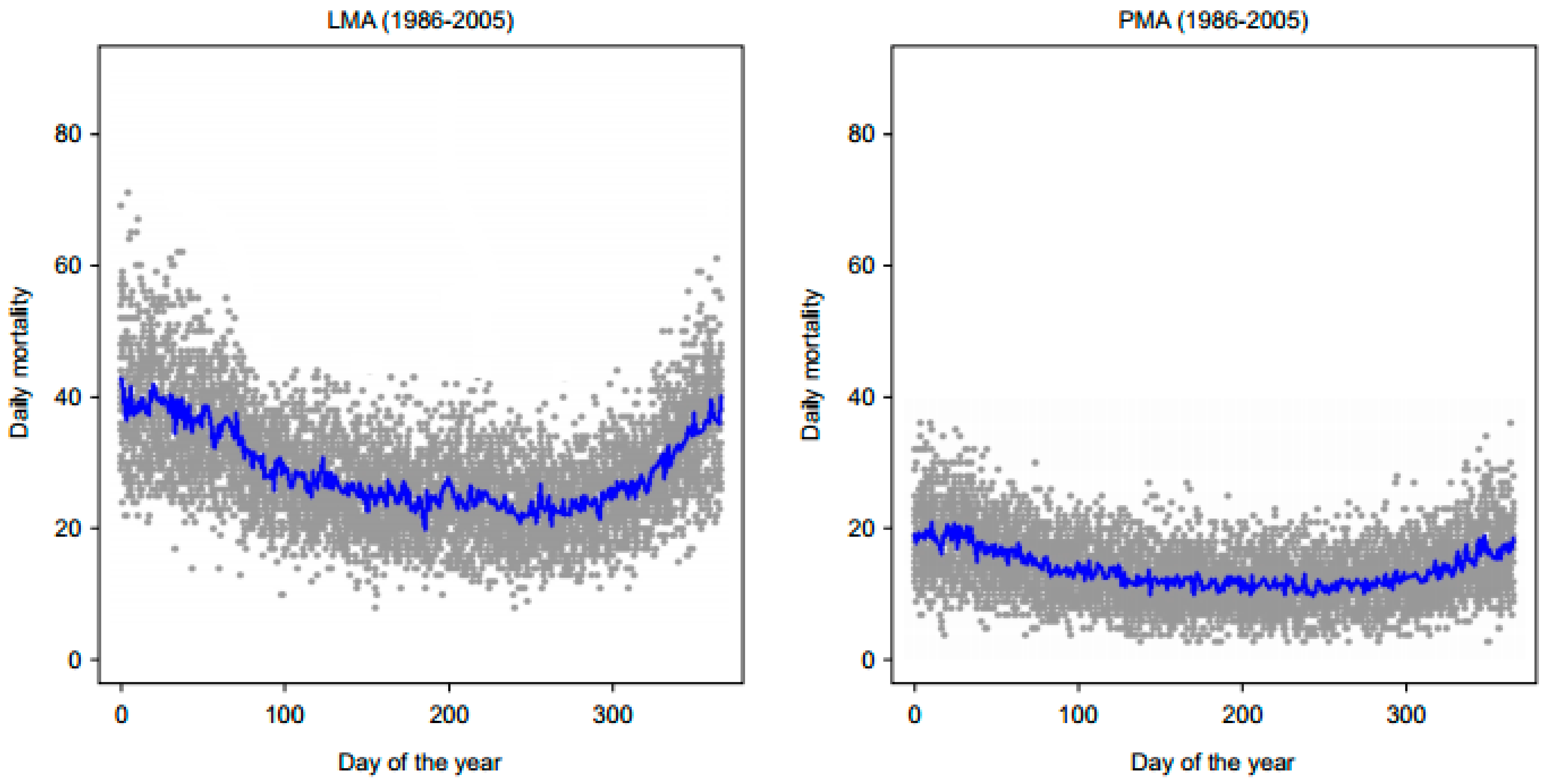
2.2. Mortality Data
2.3. Future Projected Data
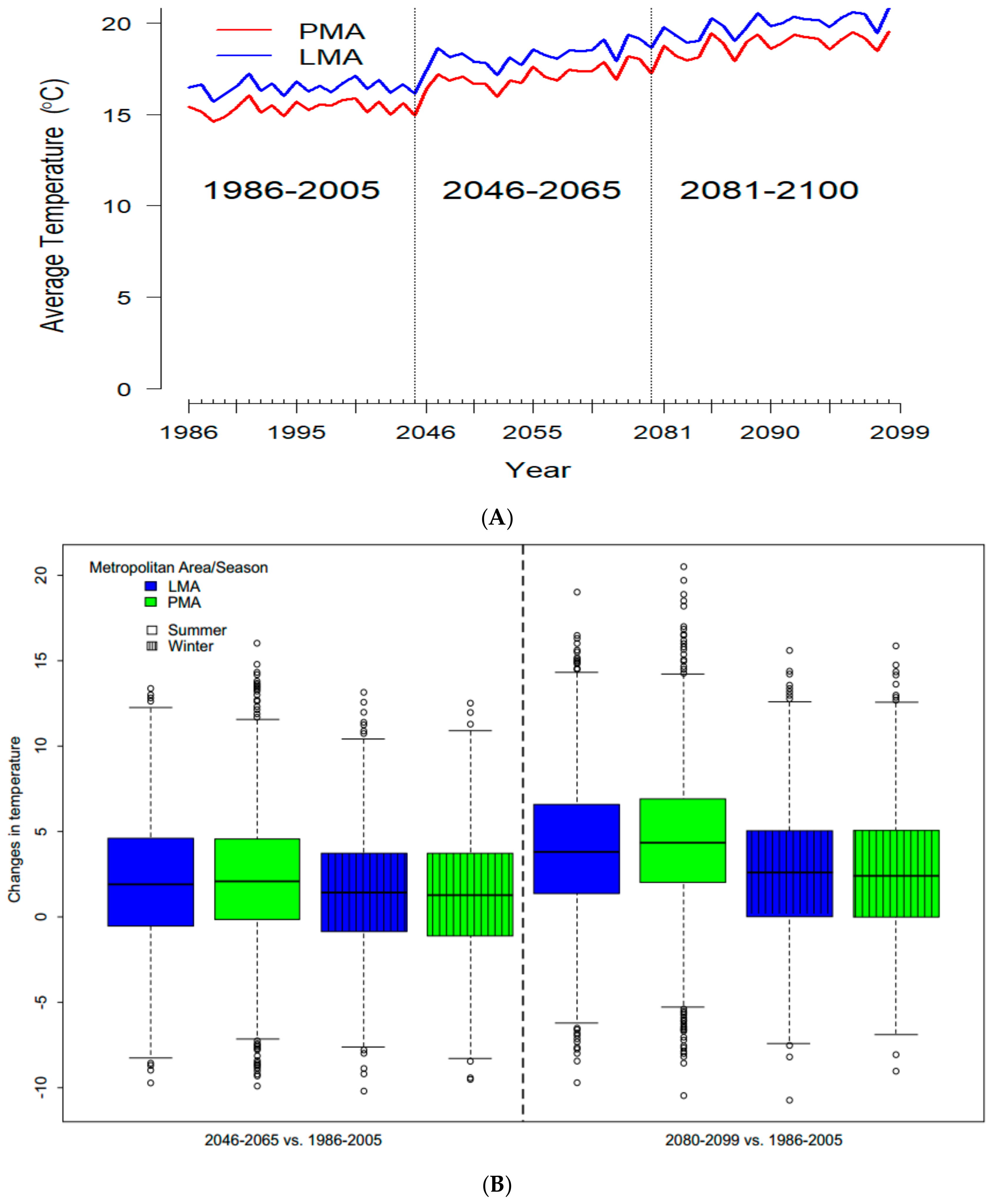
2.3.1. Temperature Projections
2.3.2. Mortality Projections
2.4. Statistical Analysis
2.4.1. Modelling the Temperature–Mortality Relationship
2.4.2. Attributable Risk from DLNMs
2.4.3. Modelling Framework and Model Assessment
3. Results
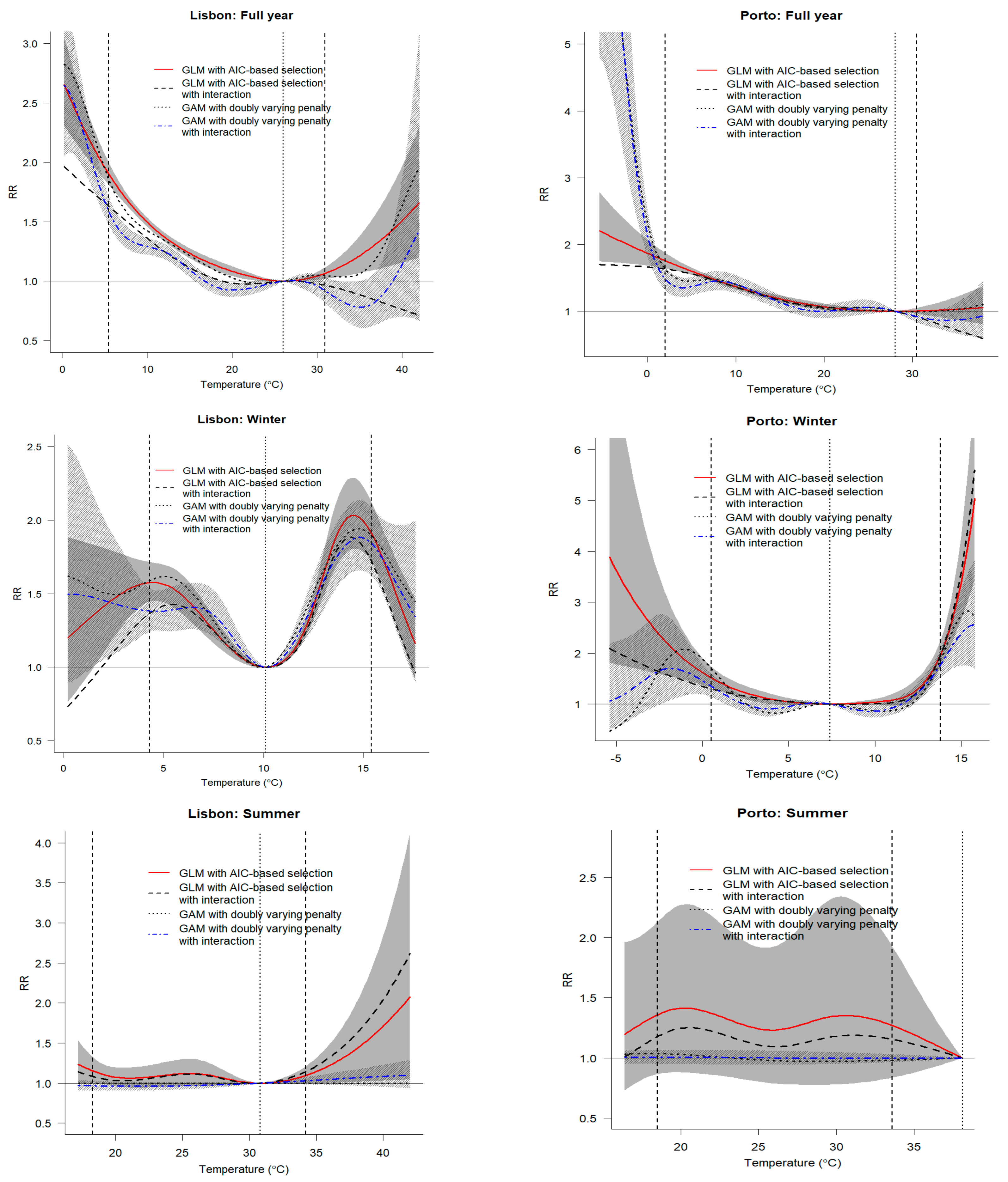
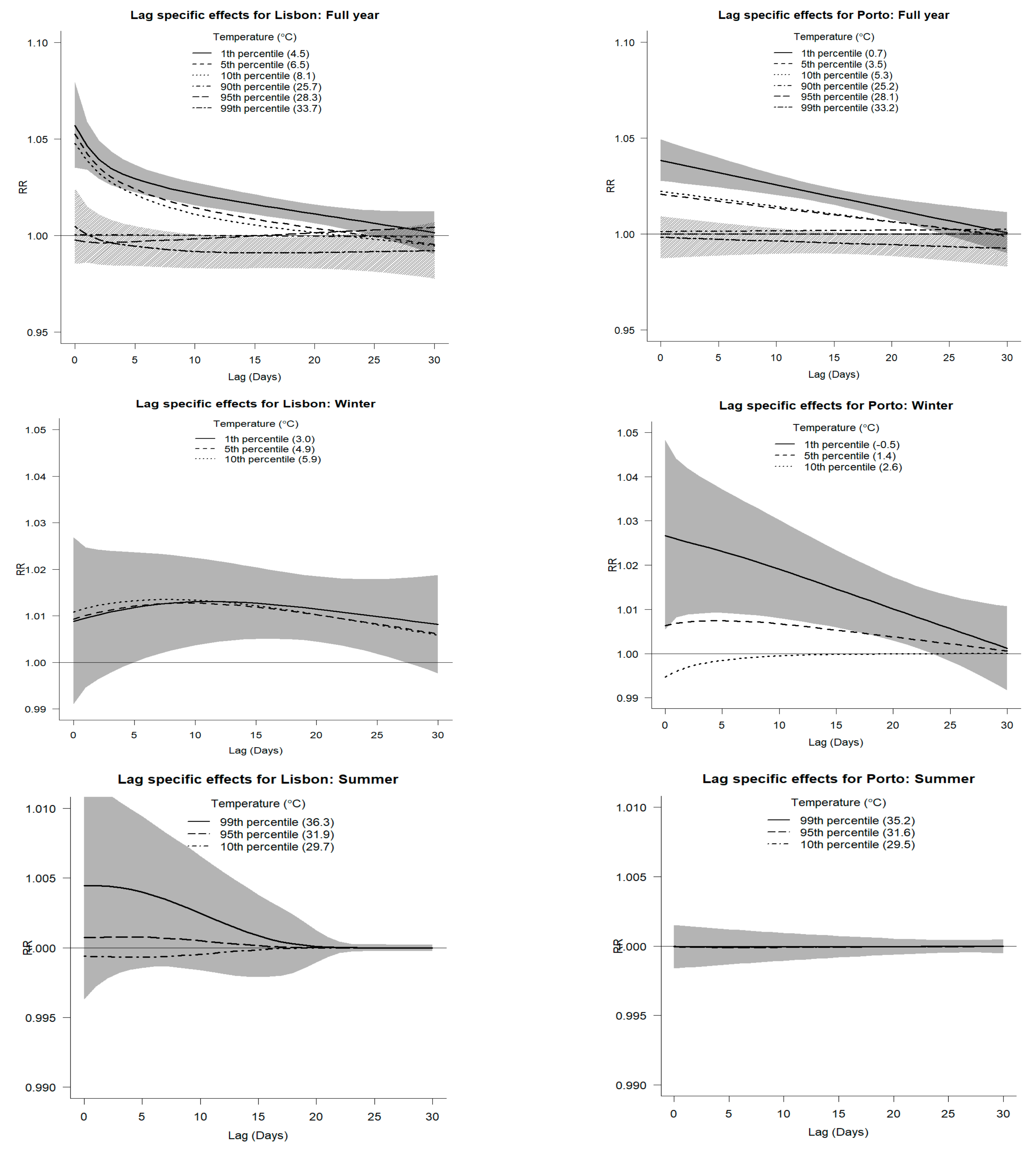
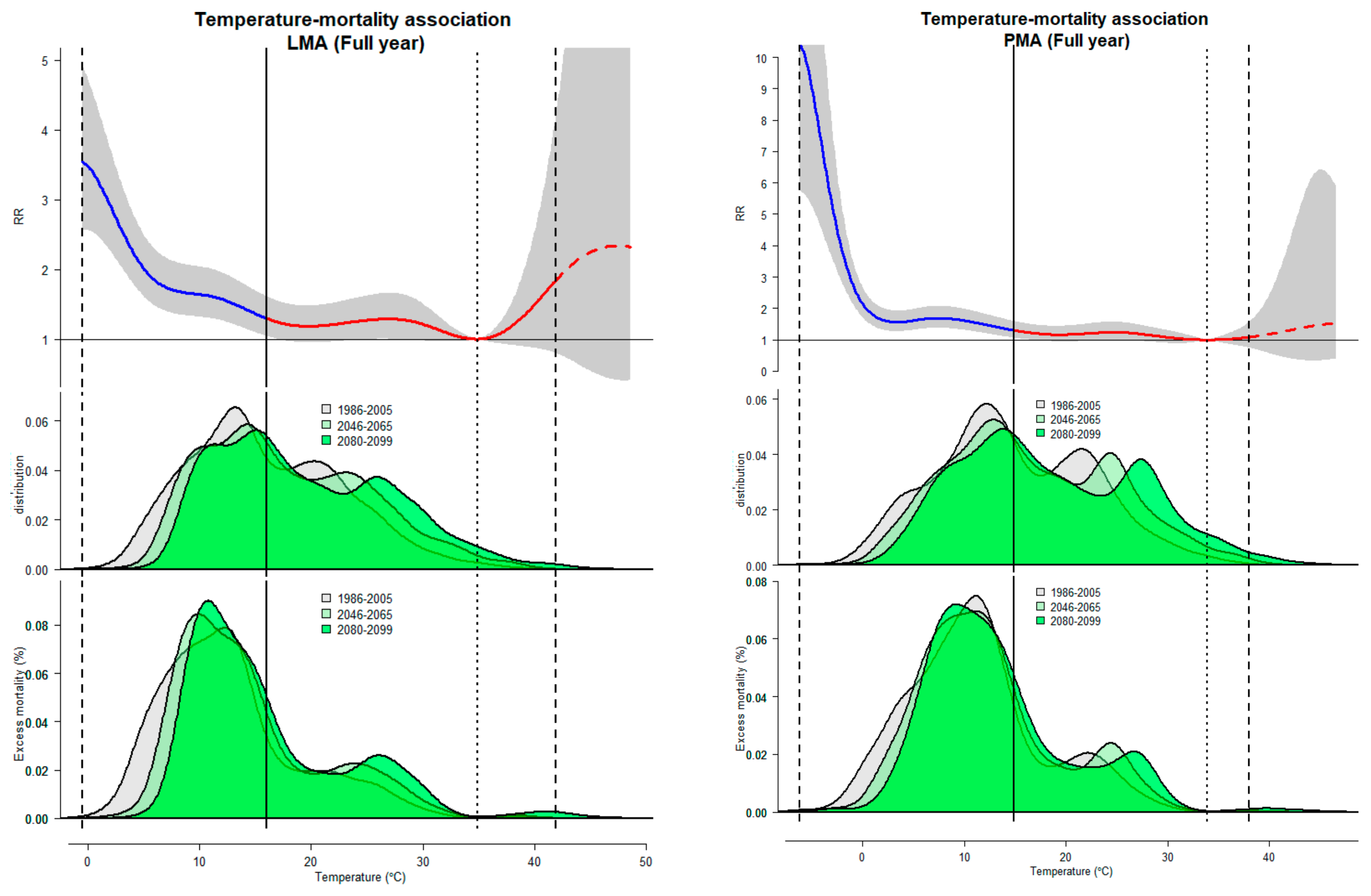
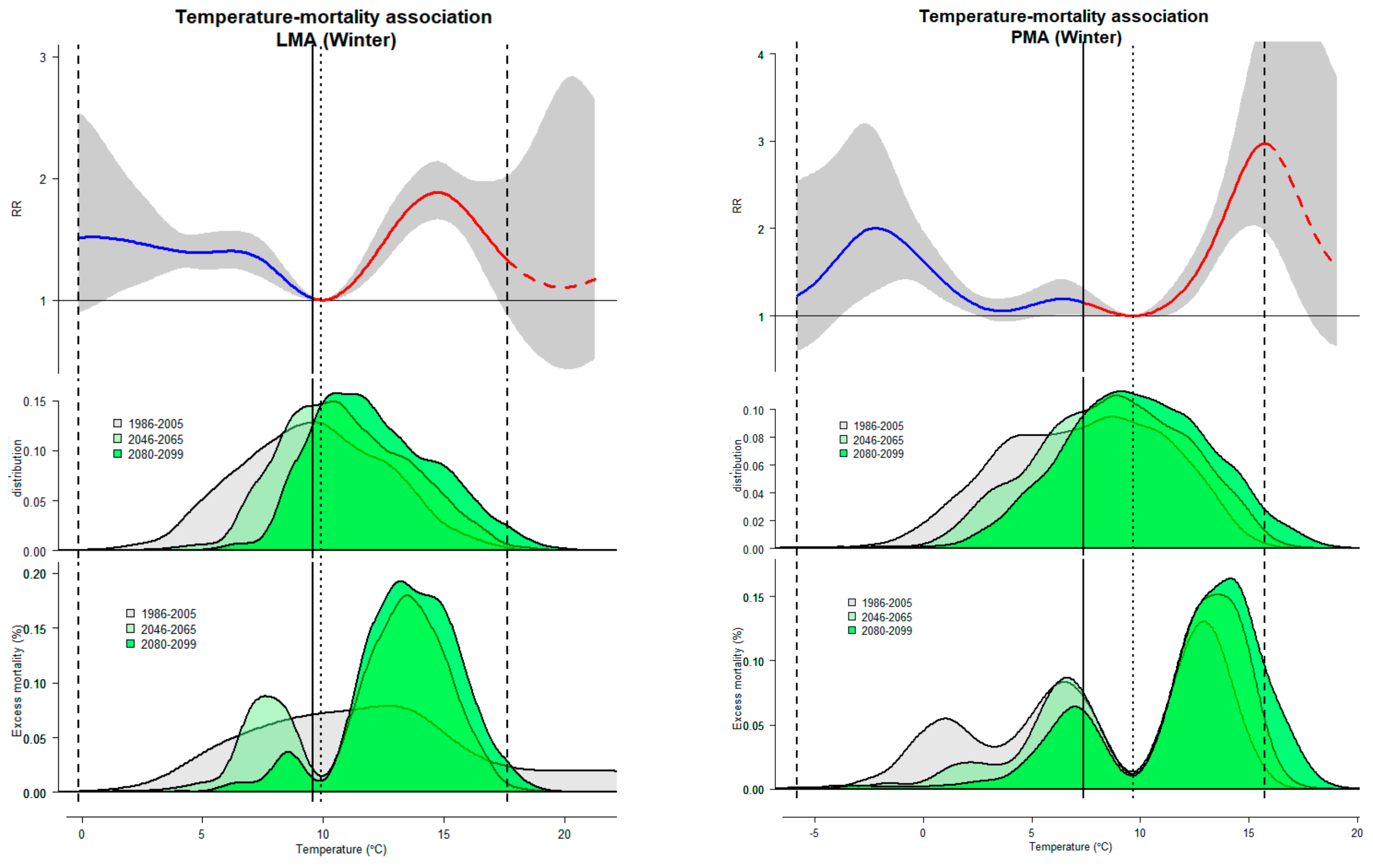
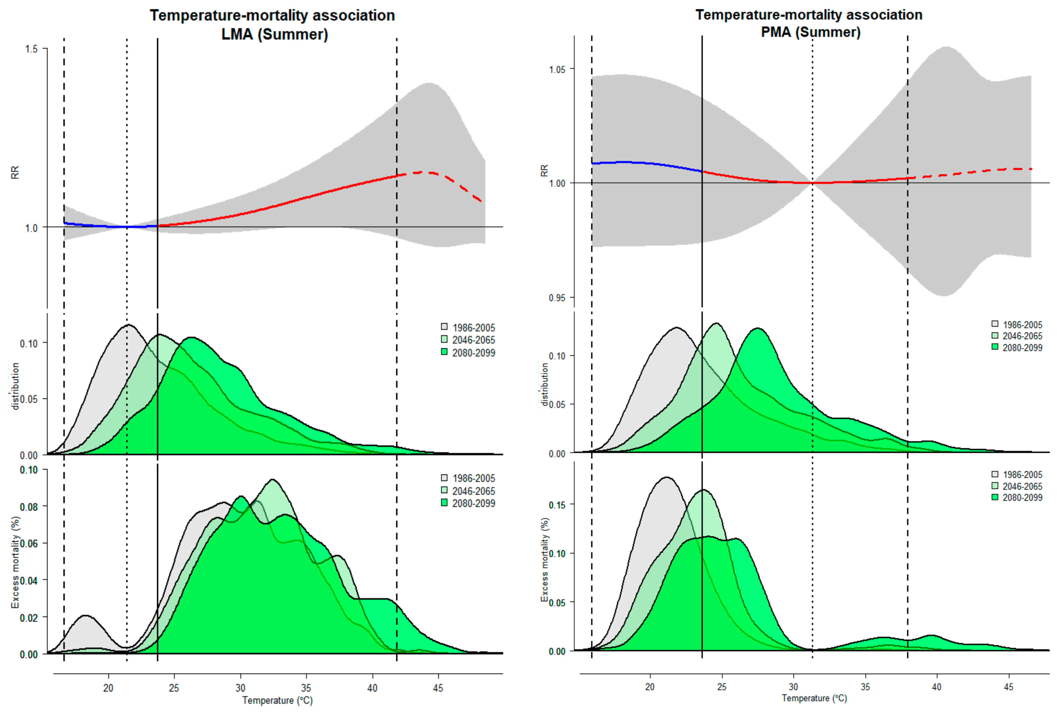
3.1. Historical Association between Temperature and Mortality
3.2. Projected Temperature-Related Mortality Rates
4. Discussion
5. Conclusions
Supplementary Materials
Author Contributions
Funding
Acknowledgments
Conflicts of Interest
References
- Gasparrini, A.; Guo, Y.; Sera, F.; Vicedo-Cabrera, A.M.; Huber, V.; Tong, S.; Coelho, M.S.Z.S.; Saldiva, P.H.N.; Lavigne, E. Projections of temperature-related excess mortality under climate change scenarios. Lancet Planet Health 2017, 1, e360–e367. [Google Scholar] [CrossRef]
- Ballester, J.; Robine, J.M.; Hermann, F.; Rodó, X. Long-term projections and acclimatization scenarios of temperature-related mortality in Europe. Nat. Commun. 2011, 2, 358. [Google Scholar] [CrossRef]
- Petkova, E.; Horton, R.; Bader, D.; Kinney, P. Projected Heat-Related Mortality in the U.S. Urban Northeast. Int. J. Environ. Res. Public Health 2013, 10, 6734–6747. [Google Scholar] [CrossRef]
- Díaz, J.; López-Bueno, J.A.; Sáez, M.; Mirón, I.J.; Luna, M.Y.; Sánchez-Martínez, G.; Carmona, R.; Barceló, M.A.; Linares, C. Will there be cold-related mortality in Spain over the 2021–2050 and 2051–2100 time horizons despite the increase in temperatures as a consequence of climate change? Environ. Res. 2019, 176, 108557. [Google Scholar] [CrossRef]
- Almendra, R.; Santana, P.; Mitsakou, C.; Heaviside, C.; Samoli, E.; Rodopoulou, S.; Vardoulakis, S. Cold-related mortality in three European metropolitan areas: Athens, Lisbon and London. Implications for health promotion. Urban Clim. 2019, 30, 100532. [Google Scholar] [CrossRef]
- Vicedo-Cabrera, A.M.; Sera, F.; Gasparrini, A. Hands-on Tutorial on a Modeling Framework for 482 Projections of Climate Change Impacts on Health. Epidemiology 2019, 30, 321–329. [Google Scholar] [CrossRef]
- Rodrigues, M.; Santana, P.; Rocha, A. Effects of extreme temperatures on cerebrovascular mortality in Lisbon: A distributed lag non-linear model. Int. J. Biometerol. 2019, 63, 549–559. [Google Scholar] [CrossRef]
- Casanueva, A.; Burgstall, A.; Kotlarski, S.; Messeri, A.; Morabito, M.; Flouris, A.D.; Nybo, L.; Spirig, C.; Schwierz, C. Overview of Existing Heat-Health Warning Systems in Europe. Int. J. Environ. Res. Public Health 2019, 16, 2657. [Google Scholar] [CrossRef]
- Morabito, M.; Crisci, A.; Moriondo, M.; Profili, F.; Francesconi, P.; Trombi, G.; Bindi, M.; Gensini, G.F.; Orlandini, S. Air temperature-related human health outcomes: Current impact and estimations of future risks in Central Italy. Sci. Total Environ. 2012, 441, 28–40. [Google Scholar] [CrossRef]
- Ravindra, K.; Rattan, P.; Mor, S.; Aggarwal, A. Generalized additive models: Building evidence of air pollution, climate change and human health. Environ. Int. 2019, 132, 104987. [Google Scholar] [CrossRef]
- Kakkoura, M.; Kouis, P.; Papatheodorou, S.I.; Paschalidou, A.K.; Ziogas, K. The effect of ambient temperature on cardiovascular and respiratory mortality in Thessaloniki, Greece. Sci. Total. Environ. 2018, 647, 1351–1358. [Google Scholar]
- Martínez, G.S.; Díaz, J.; Hooyberghs, H.; Lauwaet, D.; De Ridder, K.; Linares, C.; Carmona, R.; Ortiz, C.; Kendrovski, V.; Aerts, R.; et al. Heat and health under climate change in Antwerp: Projected impacts and implications for prevention. Environ. Int. 2018, 111, 135–143. [Google Scholar] [CrossRef] [PubMed]
- Gasparrini, A. Distributed lag linear and non-linear models in R: The package dlnm. J. Stat. Softw. 2011, 43, 1–20. [Google Scholar] [CrossRef] [PubMed]
- Neophytou, A.M.; Picciotto, S.; Brown, D.M.; Gallagher, L.E.; Checkoway, H.; Eisen, E.A.; Costello, S. Exposure-lag-response in longitudinal studies: Application of distributed lag non-linear models in an occupational cohort. Am. J. Epidemiol. 2018, 187, 1539–1548. [Google Scholar] [CrossRef] [PubMed]
- Hajat, S.; Vardoulakis, S.; Heaviside, C.; Eggen, B. Climate change effects on human health: Projections of temperature-related mortality for the UK during the 2020s, 2050s and 2080s. J. Epidemiol. Community Health 2014, 68, 641–648. [Google Scholar] [CrossRef]
- Baaghideh, M.; Mayvaneh, F. Climate Change and Simulation of Cardiovascular Disease Mortality: A Case Study of Mashhad, Iran. Iran J. Public Health 2017, 46, 396–407. [Google Scholar]
- Giang, P.N.; Dung, D.V.; Giang, K.B.; Vinhc, H.V.; Rocklöv, J. The effect of temperature on cardiovascular disease hospital admissions among elderly people in Thai Nguyen Province, Vietnam. Glob. Health Action 2014, 7, 23649. [Google Scholar] [CrossRef]
- Messner, T. Environmental variables and the risk of disease. Int. J. Circumpolar Health 2005, 64, 523–533. [Google Scholar] [CrossRef]
- Nocera, R.; Petrucelli, P.; Park, J.; Stander, E. Meteorological Variables Associated with Stroke. Int. Sch. Res. Not. 2014, 2014, 597106. [Google Scholar] [CrossRef]
- Li, T.; Horton, R.M.; Kinney, P. Future projections of seasonal patterns in temperature-related deaths for Manhattan, New York. Nat. Clim. Chang. 2013, 3, 717–721. [Google Scholar] [CrossRef]
- Baccini, M.; Kosatsky, T.; Analitis, A.; Anderson, H.R.; D’Ovidio, M.; Menne, B.; Michelozzi, P.; Biggeri, A.; PHEWE Collaborative Group. Impact of heat on mortality in 15 European cities: Attributable deaths under different weather scenarios. J. Epidemiol. Community Health 2011, 65, 64–70. [Google Scholar] [CrossRef] [PubMed]
- Kinney, P.L. Temporal Trends in Heat-Related Mortality: Implications for Future Projections. Atmosphere 2018, 9, 409. [Google Scholar] [CrossRef]
- Scovronick, N.; Sera, F.; Acquaotta, F.; Garzena, D.; Fratianni, S.; Wright, C.Y.; Gasparrini, A. The association between ambient temperature and mortality in South Africa: A time-series analysis. Environ. Res. 2018, 161, 229–235. [Google Scholar] [CrossRef] [PubMed]
- Achebak, H.; Devolder, D.; Ballester, J. Trends in temperature-related age-specific and sex-specific mortality from cardiovascular diseases in Spain: A national time-series analysis. Lancet Planet. Heal. 2019, 3, e297–e306. [Google Scholar] [CrossRef]
- Moss, R.; Babiker, M.; Brinkman, S.; Calvo, E.; Carter, T.; Edmonds, J.; Elgizouli, I.; Emori, S.; Erda, L.; Hibbard, K.; et al. Towards New Scenarios for Analysis of Emissions, Climate Change, Impacts, and Response Strategies; Intergovernmental Panel on Climate Change: Geneva, Switzerland, 2008. [Google Scholar]
- Moss, R.H.; Edmonds, J.A.; Hibbard, K.A.; Manning, M.R.; Rose, S.K.; Van Vuuren, D.P.; Carter, T.R.; Emori, S.; Kainuma, M.; Meehl, G.A.; et al. The next generation of scenarios for climate change research and assessment. Nature 2010, 463, 747. [Google Scholar] [CrossRef] [PubMed]
- Riahi, K.; Rao, S.; Krey, V.; Cho, C.; Chirkov, V.; Fischer, G.; Kindermann, G.; Nakicenovic, N.; Rafaj, P. RCP 8.5 - A scenario of comparatively high greenhouse gas emissions. Clim. Chang. 2011, 109, 33. [Google Scholar] [CrossRef]
- Intergovernmental Panel on Climate Change (IPCC). The Physical Science Basis. Contribution of Working Group I to the Fifth Assessment Report of the Intergovernmental Panel on Climate Change; Cambridge University Press: Cambridge, NY, USA, 2013; p. 1535. [Google Scholar]
- Giorgetta, M.A.; Jungclaus, J.; Reick, C.H.; Legutke, S.; Bader, J.; Bottinger, M.; Brovkin, V.; Crueger, T.; Esch, M.; Fieg, K. Climate and carbon cycle changes from 1850 to 2100 in MPI-ESM simulations for the Coupled Model Intercomparison Project phase 5. J. Adv. Model. Earth Syst. 2013, 5, 572–597. [Google Scholar] [CrossRef]
- Marta-Almeida, M.; Teixeira, J.C.; Carvalho, M.J.; Melo-Gonçalves, P.; Rocha, A.M. High resolution WRF climatic simulations for the Iberian Peninsula: Model validation. Phys. Chem. Earth 2016, 94, 94–105. [Google Scholar] [CrossRef]
- Viceto, C.; Cardoso Pereira, S.; Rocha, A. Climate Change Projections of Extreme Temperatures for the Iberian Peninsula. Atmosphere 2019, 10, 229. [Google Scholar] [CrossRef]
- Fonseca, D.; Carvalho, M.J.; Marta-Almeida, M.; Melo-Gonçalves, P.; Rocha, A. Recent trends of extreme temperature indices for the Iberian Peninsula. Phys. Chem. Earth 2016, 94, 66–76. [Google Scholar] [CrossRef]
- Pereira, S.C.; Marta-Almeida, M.; Carvalho, A.C.; Rocha, A. Heat wave and cold spell changes in Iberia for a future climate scenario. Int. J. Climatol. 2017, 37, 5192–5205. [Google Scholar] [CrossRef]
- Rodrigues, M.; Santana, P.; Rocha, A. Bootstrap approach to validate the performance of models for predicting mortality risk temperature in Portuguese metropolitan areas. Environ. Health 2019, 18, 25. [Google Scholar] [CrossRef] [PubMed]
- Gasparrini, A.; Leone, M. Attributable risk from distributed lag models. BMC Med. Res. Methodol. 2014, 14, 55. [Google Scholar] [CrossRef] [PubMed]
- Gasparrini, A.; Guo, Y.; Hashizume, M.; Lavigne, E.; Zanobetti, A.; Schwartz, J.; Tobias, A.; Tong, S.; Rocklöv, J.; Forsberg, B.; et al. Mortality risk attributable to high and low ambient temperature: A multicountry observational study. Lancet 2015, 386, 369–375. [Google Scholar] [CrossRef]
- Forzieri, G.; Cescatti, A.; Silva, F.B.; Feyen, L. Increasing risk over time of weather-related hazards to the European population: A data-driven prognostic study. Lancet Planet Health 2017, 1, e200–e208. [Google Scholar] [CrossRef]
- Weinberger, K.R.; Haykin, L.; Eliot, M.N.; Schwartz, J.D.; Gasparrini, A.; Wellenius, G.A. Projected temperature-related deaths in ten large US metropolitan areas under different climate change scenarios. Environ. Int. 2017, 107, 196–204. [Google Scholar] [CrossRef]
- Guo, Y.; Barnett, A.G.; Tong, S. High temperatures-related elderly mortality varied greatly from year to year: Important information for heat-warning systems. Sci. Rep. 2012, 2, 830. [Google Scholar] [CrossRef]
- Martínez-Solanas, E.; Basagaña, X. Temporal changes in temperature-related mortality in Spain and effect of the implementation of a Heat Health Prevention Plan. Environ. Res. 2018, 169, 102–113. [Google Scholar] [CrossRef]
- Benmarhnia, T.; Bailey, Z.; Kaiser, D.; Auger, N.; King, N.; Kaufman, J.S. A difference-in-differences approach to assess the effect of a heat action plan on heat-related mortality, and differences in effectiveness according to sex, age, and socioeconomic status (Montreal, Quebec). Environ. Health Perspect. 2016, 124, 1694–1699. [Google Scholar] [CrossRef]
- Knowlton, K.; Lynn, B.; Goldberg, R.A.; Rosenzweig, C.; Hogrefe, C.; Rosenthal, J.K.; Kinney, P.L. Projecting heat-related mortality impacts under a changing climate in the New York City region. Am. J. Public Health 2007, 97, 2028–2034. [Google Scholar] [CrossRef]
- Gasparrini, A.; Scheipl, F.; Armstrong, B.; Kenward, M.G. A penalized framework for distributed lag non-linear models. Biometrics 2017, 73, 938–948. [Google Scholar] [CrossRef]
- DGS—Direção Geral de Saúde. Plano de Contingência para Temperaturas Extremas Adversas—Módulo de Calor 2014. Available online: https://www.dgs.pt/documentos-e-publicacoes/plano-de-contingencia-para-temperaturas-extremas-adversas-modulo-calor-2014.aspx (accessed on 18 September 2019).
- DGS—Direção Geral de Saúde. Plano de Contingência Para Temperaturas Extremas Adversas—Módulo Inverno 2016. Available online: https://www.dgs.pt/documentos-e-publicacoes/saude-sazonal-inverno-saude-.aspx (accessed on 18 September 2019).
- Watts, N.; Amann, M.; Arnell, N.; Ayeb-Karlsson, S.; Belesova, K.; Berry, H.; Bouley, T.; Boykoff, M.; Byass, P.; Cai, W.; et al. The 2018 report of the Lancet Countdown on health and climate change: Shaping the health of nations for centuries to come. Lancet 2018, 392, 2479–2514. [Google Scholar] [CrossRef]
- Martinez, G.S.; Linares, C.; Ayuso, A.; Kendrovski, V.; Boeckmann, M.; Diaz, J. Heat-health action plans in Europe: Challenges ahead and how to tackle them. Environ. Res. 2019, 176, 108548. [Google Scholar] [CrossRef]
- Sheridan, S.C.; Kalkstein, L.S. Progress in heat watch-warning system technology. Bull. Am. Meteorol. Soc. 2004, 85, 1931–1941. [Google Scholar] [CrossRef]
- Lowe, D.; Ebi, K.; Forsberg, B. Heatwave early warning systems and adaptation advice to reduce human health consequences of heatwaves. Int. J. Environ. Res. Public Health 2011, 8, 4623–4648. [Google Scholar] [CrossRef]


| Metropolitan Area | Season | Total Deaths | Daily Temperature † (1986–2005) | Projected Temperature (2046–2065) | Projected Temperature (2080–2099) | d MMT (95% CI) |
|---|---|---|---|---|---|---|
| Lisbon | Full year | 209,964 | 15.4 (11.4–21.3) a | 17.0 (12.6–23.7) | 18.5 (13.7–25.8) | 26 (24.8–27.1) |
| Summer | 58,376 | 23.3 (21.1–26.4) c | 25.8 (23.4–28.8) | 28.1 (25.7–31.1 | ||
| Winter | 86,559 | 9.8 (7.6–11.9) b | 10.9 (9.2–13.0) | 12.0 (10.4–14.2) | ||
| Porto | Full year | 100,280 | 14.5 (10.0–26.0) a | 15.9 (11.0–23.7) | 17.5 (12.2–26.3) | 29.9 (24.1–41.5) |
| Summer | 28,029 | 23.1 (21.2–26.0) c | 25.5 (23.6–28.8) | 28.2 (26.2–31.2) | ||
| Winter | 40,722 | 7.8 (4.7–10.4) b | 8.9 (6.4–11.3) | 10.0 (7.7–12.4) |
| Metropolitan Area/Season | Temperature | RR (95% CI) | AN (95% eCI) | AF% (95% eCI) | AF rel (%) |
|---|---|---|---|---|---|
| Historical (1986–2005) | |||||
| Lisbon/Full year | 1th percentile: 4.5 | 2.30 (1.84, 2.88) | 1546.67 (1294.51, 1730.92) | 0.74 (0.62, 0.82) | 0 |
| 99th percentile: 33.7 | 1.03 (0.96, 1.09) | 92.70 (−34.73, 183.78) | 0.04 (−0.02, 0.09) | 0 | |
| Lisbon/Winter | 1th percentile: 3.0 | 1.45 (1.16, 1.82) | 1894.54 (1378.90, 2312.19) | 0.67 (0.49, 0.82) | 0 |
| 99th percentile: 16.3 | 1.67 (1.41, 1.99) | 316.47 (145.23, 451.03) | 0.11 (0.05, 0.16) | 0 | |
| Lisbon/Summer | 1th percentile: 17.7 | 1.01 (0.97, 1.05) | 37.98 (−227.48, 294.64) | 0.02 (−0.14, 0.18) | 0 |
| 99th percentile: 36.3 | 1.09 (1.00, 1.19) | 59.39 (−2.66, 116.64) | 0.04 (0.00, 0.07) | 0 | |
| Porto/Full year | 1th percentile: 0.70 | 2.07 (1.66, 2.58) | 811.95 (691.33, 910.25) | 0.81 (0.69, 0.91) | 0 |
| 99th percentile: 33.30 | 1.00 (0.95, 1.06) | 8.64 (−47.03, 54.79) | 0.01 (−0.05, 0.05) | 0 | |
| Porto/Winter | 1th percentile: −0.5 | 1.82 (1.41, 2.34) | 382.95 (−108.21, 802.38) | 0.14 (−0.04, 0.28) | 0 |
| 99th percentile: 14.4 | 2.43 (1.91, 3.10) | 2868.99 (2093.18, 3374.93) | 1.02 (0.74, 1.20) | 0 | |
| Porto/Summer | 1th percentile: 18 | 1.01 (0.97, 1.05) | 5.86 (−25.46, 34.17) | 0 (−0.02, 0.02) | 0 |
| 99th percentile: 35.2 | 1.00 (0.98, 1.02) | 14.28 (−69.73, 89.78) | 0.01 (−0.04, 0.05) | 0 | |
| Future (2046–2065) | |||||
| Lisbon/Full year | 1th percentile: 6.9 | 1.81 (1.45, 2.25) | 231.83 (193.49, 259.78) | 0.11 (0.09, 0.12) | −0.63 (−0.7, −0.52) |
| 99th percentile: 36.4 | 1.03 (0.95, 1.12) | 298.43 (−118.67, 592.22) | 0.14 (−0.06, 0.28) | 0.10 (−0.04, 0.19) | |
| Lisbon/Winter | 1th percentile: 5.5 | 1.39 (1.25, 1.55) | 259.29 (189.10, 316.34) | 0.09 (0.07, 0.11) | −0.58 (−0.71, −0.42) |
| 99th percentile: 17.1 | 1.47 (1.10, 1.98) | 887.76 (264.19, 1308.12) | 0.31 (0.09, 0.46) | 0.20 (0.04, 0.30) | |
| Lisbon/Summer | 1th percentile: 19.1 | 1.00 (0.98, 1.03) | 9.50 (−60.04, 79.43) | 0.01 (−0.04, 0.05) | −0.02 (−0.13, 0.10) |
| 99th percentile: 38.4 | 1.11 (1.00, 1.25) | 188.91 (−9.35, 371.79) | 0.11 (−0.01, 0.22) | 0.08 (0.00, 0.15) | |
| Porto/Full year | 1th percentile: 2.5 | 1.64 (1.33, 2.03) | 192.51 (168.52, 209.75) | 0.19 (0.17, 0.21) | −0.62 (−0.70, −0.52) |
| 99th percentile: 36.4 | 1.03 (0.85, 1.24) | 54.82 (−259.08, 292.64) | 0.05 (−0.26, 0.29) | 0.05 (−0.22, 0.24) | |
| Porto/Winter | 1th percentile: 1.3 | 1.37 (1.17, 1.61) | 49.95 (−13.44, 105.34) | 0.02 (0.00, 0.04) | −0.12 (−0.25, 0.03) |
| 99th percentile: 15.4 | 2.92 (2.03, 4.19) | 6459.91 (4563.58, 7642.42) | 2.29 (1.62, 2.71) | 1.27 (0.88, 1.52) | |
| Porto/Summer | 1th percentile: 19.1 | 1.01 (0.97, 1.05) | 0.45 (−2.02, 2.68) | 0 (0.00, 0.00) | 0 (−0.02, 0.01) |
| 99th percentile: 37.5 | 1.00 (0.97, 1.04) | 21.85 (−122.99, 157.10) | 0.01 (−0.07, 0.09) | 0.00 (−0.04, 0.04) | |
| Future (2080–2099) | |||||
| Lisbon/Full year | 1th percentile: 8.6 | 1.69 (1.36, 2.10) | 25.03 (20.45, 28.34) | 0.01 (0.01, 0.01) | −0.73 (−0.81, −0.61) |
| 99th percentile: 39.4 | 1.37 (0.89, 2.10) | 1050.35 (−462.24, 1898.65) | 0.50 (−0.22, 0.90) | 0.46 (−0.21, 0.82) | |
| Lisbon/Winter | 1th percentile: 7.1 | 1.38 (1.23, 1.55) | 23.42 (16.53, 29.06) | 0.01 (0.01, 0.01) | −0.66 (−0.81, −0.48) |
| 99th percentile: 18.5 | 1.20 (0.65, 2.22) | 1820.53 (−387.48, 3054.90) | 0.65 (−0.14, 1.08) | 0.53 (−0.18, 0.92) | |
| Lisbon/Summer | 1th percentile: 20.6 | 1.00 (0.99, 1.01) | 1.10 (−8.91, 10.95) | 0.00 (−0.01, 0.01) | −0.02 (−0.17, 0.13) |
| 99th percentile: 42.2 | 1.14 (0.97, 1.36) | 444.65 (−30.75, 891.90) | 0.27 (−0.02, 0.54) | 0.23 (−0.02, 0.47) | |
| Porto/Full year | 1th percentile: 3.9 | 1.56 (1.27, 1.93) | 120.83 (105.94, 131.60) | 0.12 (0.11, 0.13) | −0.69 (−0.78, −0.58) |
| 99th percentile: 39.3 | 1.14 (0.65, 1.99) | 216.01 (−1004.00, 890.65) | 0.22 (−1.00, 0.89) | 0.21 (−0.98, 0.83) | |
| Porto/Winter | 1th percentile: 2.8 | 1.11 (1.00, 1.24) | 5.14 (−5.64, 14.37) | 0.00 (0.00, 0.01) | −0.13 (−0.28, 0.04) |
| 99th percentile: 17.1 | 2.49 (1.36, 4.56) | 10761.18 (6706.74, 13068.30) | 3.81 (2.38, 4.63) | 2.80 (1.63, 3.44) | |
| Porto/Summer | 1th percentile: 20.6 | 1.01 (0.97, 1.05) | 0.24 (−2.53, 3.29) | 0 (0.00, 0.00) | 0 (−0.02, 0.02) |
| 99th percentile: 41.2 | 1.00 (0.95, 1.06) | 24.58 (−158.76, 187.31) | 0.01(−0.10, 0.11) | 0.01 (−0.06, 0.06) |
© 2019 by the authors. Licensee MDPI, Basel, Switzerland. This article is an open access article distributed under the terms and conditions of the Creative Commons Attribution (CC BY) license (http://creativecommons.org/licenses/by/4.0/).
Share and Cite
Rodrigues, M.; Santana, P.; Rocha, A. Projections of Temperature-Attributable Deaths in Portuguese Metropolitan Areas: A Time-Series Modelling Approach. Atmosphere 2019, 10, 735. https://doi.org/10.3390/atmos10120735
Rodrigues M, Santana P, Rocha A. Projections of Temperature-Attributable Deaths in Portuguese Metropolitan Areas: A Time-Series Modelling Approach. Atmosphere. 2019; 10(12):735. https://doi.org/10.3390/atmos10120735
Chicago/Turabian StyleRodrigues, Mónica, Paula Santana, and Alfredo Rocha. 2019. "Projections of Temperature-Attributable Deaths in Portuguese Metropolitan Areas: A Time-Series Modelling Approach" Atmosphere 10, no. 12: 735. https://doi.org/10.3390/atmos10120735
APA StyleRodrigues, M., Santana, P., & Rocha, A. (2019). Projections of Temperature-Attributable Deaths in Portuguese Metropolitan Areas: A Time-Series Modelling Approach. Atmosphere, 10(12), 735. https://doi.org/10.3390/atmos10120735