Abstract
Climate studies based on global climate models (GCMs) project a steady increase in annual average temperature and severe heat extremes in central North America during the mid-century and beyond. However, the agreement of observed trends with climate model trends varies substantially across the region. The present study focuses on two different locations: Des Moines, IA and Austin, TX. In Des Moines, annual extreme temperatures have not increased over the past three decades unlike the trend of regionally-downscaled GCM data for the Midwest, likely due to a “warming hole” over the area linked to agricultural factors. This warming hole effect is not evident for Austin over the same time period, where extreme temperatures have been higher than projected by regionally-downscaled climate (RDC) forecasts. In consideration of the deviation of such RDC extreme temperature forecasts from observations, this study statistically analyzes RDC data in conjunction with observational data to define for these two cities a 95% prediction interval of heat extreme values by 2040. The statistical model is constructed using a linear combination of RDC ensemble-member annual extreme temperature forecasts with regression coefficients for individual forecasts estimated by optimizing model results against observations over a 52-year training period.
1. Introduction
Extreme urban heat events can have significant societal impact. They not only cause serious health risks [1,2] but they strain the existing energy infrastructure in the United States (U.S.). Nearly three-fourths of all U.S. electricity is associated with buildings [3]; approximately 86% of all buildings use air conditioning [4]. Thus, extreme heat events not only result in increased electricity loads due to a high demand for residential and commercial building cooling but they also impact electricity generation, distribution, and transmission [5]. During a heat wave, electricity generation can be reduced by more than 1% per 1 °C temperature increase [6].
For purposes of long-term electricity generation planning, the energy sector is dependent on reliable projections of future heat extreme events. Studies using global climate models (GCMs) predict increased average temperatures for mid-latitude localities (within a range of 1.5–5 °C) in North America from 1990 to the current mid-century [7,8,9,10]. Along with an increase in average temperature, an increase in extreme heat events is also projected, both in terms of peak temperature and frequency. By mid-century, the annual average number of days with temperatures exceeding 37.8 °C (100 °F) is predicted to more than double in the Great Plains as compared to the end of the previous century. This increase will occur even with a substantial reduction in greenhouse gas emissions [11] (p. 444).
GCM projections, however, can deviate from what is observed for specific locations. Due to the urban heat island effect, as has been documented in various studies [12,13,14,15], temperatures are anticipated to be even higher for areas of increased urbanization. On the other hand, it has been shown that between 1981–1990 the maximum number of annually averaged temperatures from GCM data tend to be 1 °C higher than actual observations for cities in the large crop-producing region of central North America. In the last quarter of the past century, these cities have shown a cooling trend by as much as 0.8 °C [8,16,17] (p. 190). This apparent discrepancy in temperatures among climate models and observations is associated with a “warming hole” in the Midwest [18,19]. Pan et al. (2004) [16] propose that changes in the low-level jet frequency in the central U.S. have resulted in stronger moisture convergence and higher precipitation in the upper Midwest and thus in enhanced evapotranspiration and reduced surface warming in the summer. Mueller et al. (2015) [20] offer evidence that cropland intensification (such as growing crops with a larger leaf area index and increased photosynthetic rates) and the associated increase in evapotranspiration causes a reduction in summer temperature extremes and more precipitation in the Midwest. Their study also shows that in times of drought for non-irrigated regions, evapotranspiration is reduced, thus allowing for higher peak temperatures during heat waves.
It is not surprising that GCM models with a spatial resolution of 1–2° do not account well for local regional effects. Regionally downscaled climate (RDC) datasets, such as through the coupled model intercomparison project phase 5 (CMIP5) multi-model ensemble [21,22], are available. However, even if at a spatial resolution of 1/8°, RDC data cannot recoup relatively small-scale (i.e., regional) signatures if they are not present in the source GCM data. It is true that certain bias-correction techniques are used to construct these RDC datasets [23,24], but the effectiveness of such techniques must be analyzed region by region. Here, the focus is on the appropriateness of using RDC data to account for future extreme high temperature projections specifically for the central U.S., which involves a comparison of historical RDC temperature forecasts with observations over previous decades.
A divergence between RDC data and observations would suggest that it is important to incorporate not only RDC temperature forecast trends but also past observations to project the occurrence of future heat extremes for specific localities. The objective of this study is to identify the most likely ranges of annual peak temperatures (defined by a 95% prediction interval, PI) by mid-century in urban areas by incorporating both RDC and observational data. We present a statistical model based on the ensemble model output statistics (EMOS) method [25] that can calibrate RDC projections with observations. Among available RDC projections, we select the most influential to improve predictions in future years.
Two cities in the central U.S.—Des Moines, Iowa and Austin, Texas—are considered here. The Austin metro area has a population of around two million; the Des Moines metro is about one-third that, although their urban population densities are similar, with 2500 people per square mile in Des Moines and a population density that is roughly 30% higher in Austin [26,27]. Both cities are similar in their summer weather in that mid-summers are very warm to hot, and rather humid. One key difference is that cold frontal passages occur in Des Moines from time to time allowing some periods of cooler weather, which are much rarer in Austin. Therefore, the average July temperature in Austin of about 35 °C is 4 °C higher than the 31 °C average July temperature in Des Moines [28].
These two cities were selected, in particular, because of the availability of detailed data relating to energy use and because both will be used in a subsequent study of urban energy use during future extreme heat events. The study will compare trends seen in both the observational record and climate model projections to determine if a single best approach would work in both cities for statistically modeling plausible values of future annual peak temperatures, and to compensate for apparent inadequacies in the ability of RDC forecasts to account for the Midwest warming hole and urban heat island effects.
In Section 2, we describe the RDC and observational data used for Des Moines and Austin as well as the theoretical basis for the EMOS statistical model used to predict the future range in annual heat extremes. In Section 3, we discuss the means for formulating the EMOS model as appropriate for both cities and the resultant 95% PI on annual peak temperatures for both cities by mid-century. A summary of results is given in Section 4 along with implications for the energy sector.
2. Data and Methodology
This work is motivated by a larger project focused on the projected energy use and peak energy demands of urban areas, specifically Des Moines and Austin, during heat extreme events from the present to 2040. This year was arbitrarily chosen; it coincides with the year that a draft U.N. report projects global warming will result in an exceedance of the average global temperature ceiling as set by the Paris Agreement [29]. Given the projected increase in average temperatures for central North America, it could be anticipated that an increase in extreme heat wave temperatures will also occur. To investigate a “most likely” range of extreme high temperatures by 2040, this study investigates the long-term trends during a historical period (1950–2017) in both observational and climate model forecasts as well as trends projected by climate models through 2040.
2.1. Data
Recorded temperatures at 2 m above ground level (AGL) are acquired from Automatic Sensing Observing Systems (ASOS) stations in Austin and Des Moines [30]. ASOS provide a continuous record of daily maximum high and low temperatures since 1950 for both cities. The Austin ASOS site KATT (latitude 30.32°, longitude –97.76°) was selected among other ASOS sites in the metro area because it is in a region of higher urban density compared to the other sites. The single Des Moines ASOS site KDSM (latitude 41.53°, longitude –93.66°) is located at the commercial airport on the south side of the urban area.
The RDC data used here originates from the CMIP5 multi-model ensemble, as previously mentioned. These RDC datasets have a spatial resolution of 1/8° and provide climate projections of daily maximum temperature (among other variables) for the period from 1950 to 2100. RDC datasets were contributed by a number of meteorological entities worldwide using different configurations of 15 different climate models (Table 1) to generate an ensemble of multiple climate projections. Ensemble members exist for climates with predefined future projections of greenhouse gas (GHG) concentration known as representative concentration pathways (RCP) [31]. RDC ensembles based on two specific RCP scenarios are considered here, which represent GHG concentrations and associated radiative forcing that either increase through mid-century but then stabilize (RCP4.5) or continue increasing throughout the century (RCP8.5). Among the range of RCP scenarios, these two are chosen to represent a moderate mitigation scenario (RCP4.5) and worst-case (RCP8.5) climate scenario. Under RCP 4.5 (8.5) scenario, 42 (41) RDC projections are used in this study. Time series of annual maximum temperature are extracted respectively for both cities from RDC data at a single grid point closest to the latitude and longitude locations of the two ASOS sites, KATT and KDSM.

Table 1.
List of models contributing to CMIP5 GCM and associated RDC model data used.
Figure 1 presents annual high temperature extremes from the full ensemble set of RDC projections as well as ASOS observations for both Des Moines and Austin since 1950. ASOS observations are given through 2017. Analysis of these data and the means for identifying most likely high extreme temperatures by 2040 for Des Moines and Austin are described in subsequent sections.
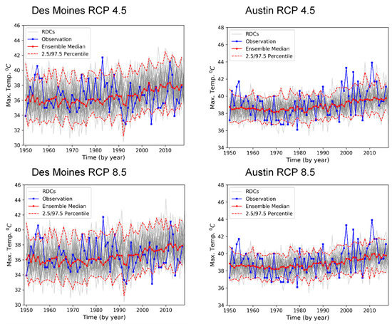
Figure 1.
Annual peak temperatures from RDC ensemble data (light gray) and ASOS observations (dark blue) for Des Moines (left) and Austin (right) and by climate scenarios of RCP 4.5 (top row) and RCP 8.5 (bottom row) showing also RDC ensemble median (red line) with ensemble 2.5 and 97.5 percentile values (pink dashed lines).
2.2. Comparison of Observed and RDC Forecast Annual Heat Extremes
To compare RDC forecast performance to observations, least-squares quadratic trends are formulated based on times series data of observed and RDC forecast annual peak temperatures for the historical period (1950–2017) for both cities. Considering the 42 (41) RDC projections for RCP 4.5 (8.5) available, we calculate two quadratic trends of the RDC projections. First, observations are compared against the mean trend across the 42 (41)-member ensemble. Second, we fit a trend using projections from the “best fit” RDC member, which has the smallest mean absolute error relative to observations during the historical period (1950–2017). The results suggest that the trend predicted by RDC projections do not agree with the trend from observations, as shown in detail in Section 3.1. In the following section, we propose a new method that supplements RDC projections with actual observations.
2.3. EMOS Method for Defining Most Likely Future Heat Extremes
In order to identify an envelope of values that define a “most likely” range of annual maximum temperatures by 2040, it is necessary to project the RDC data ensemble mean and variance (or uncertainty) of annual temperature extremes into the future. However, it is also necessary to consider RDC data deviation (if any) from observations during the historical period. Here, an ensemble of multiple RDC projections is considered along with observational data as part of an integrative statistical approach known as the EMOS method, which was previously mentioned. The EMOS approach uses a parametric distribution, such as a normal, truncated normal, log-normal, or generalized extreme value distribution, or a combination thereof, to make predictions [25,32,33,34,35]. For temperature predictions as considered here, the overall forecast is formulated as a linear combination of M individual RDC forecasts called covariates or predictors. Specifically, the annual maximum temperature, , for a given year is modeled by:
where is the annual peak temperature from the th RDC projection in year t, and the error term, , is assumed to follow a normal distribution with zero mean. The coefficients, , can be estimated using linear regression. The original EMOS approach assumes that the variance of increases, as the variability of RDC forecasts increases, that is, where denotes the ensemble variance and c and d are nonnegative coefficients. However, our analysis shows that the variability of the annual peak temperature is not necessarily correlated with the ensemble variance. Therefore, we employ a constant variance in our analysis, that is,
The typical EMOS approach uses all the ensemble covariates, which consists of 42 (41) RDC projections for RCP 4.5 (8.5) in our case. However, when a relatively large number of covariates are included, there exists the possibility of overfitting, such that the predictive model conforms nearly identically to historical data points during the training period but the model forecast can degrade significantly over the testing period [36].
To avoid overfitting, one remedy is to use penalized regression—e.g., Ridge regression [37] or least absolute shrinkage and selection operator (LASSO) regression [38]—which imposes a penalty on the number and/or magnitude of the regression coefficients employed, a process that typically requires additional splitting of the dataset for cross validation to identify the regularization parameter. Preliminary work using annual extreme temperature RDC data for Austin and Des Moines since 1950 (not shown here) to evaluate the effectiveness of LASSO and Ridge regression techniques for identifying appropriate model covariates revealed that both techniques help to avoid overfitting. These methods can provide a simpler model than results when one uses all RDC covariates and can improve overall prediction capability. However, these penalized regression approaches do not provide a PI in closed form, because the estimated regression coefficients associated with their use are biased [39]. Another approach to prevent overfitting is to use a variable selection method such as forward selection. Our analysis also showed that application of the forward selection procedure results in the need for no fewer than 20 covariates (RDC forecasts) for both cities, which still leads to some overfitting.
In order to determine the appropriate number of covariates and include only those that are most influential for the model solution, it was decided here to use a cross-validation technique—in particular, the leave-one-out cross-validation (LOOCV) technique. This technique uses the data points in the training period for suitably selecting covariates with respect to observations [35,39]. In our analysis, we use 1950–2002 as the model training period. Suppose we use data points (years) in the model training period, over which the LOOCV technique is applied. Here, data points are used for fitting the model, while the remaining one data point, treated as the validation data point, is used for evaluating the prediction error. We repeat this procedure times with all the different validation data points (Figure 2) and compute the MSE using all the validation data points as follows:
where is the observed annual peak temperature at the th validation data point and represents its predicted annual peak temperature.
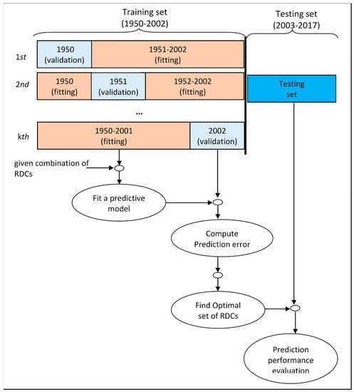
Figure 2.
The LOOCV procedure for covariate selection and model evaluation when data in 1950–2002 are used for training in the prediction model (modified based on a figure originally available in Byon et al. 2010. [40]).
To select the best model, one that generates the lowest MSE in the LOOCV, would require comparison of all possible model alternatives. With 42 (41) covariates for RCP 4.5 (RCP 8.5), such a full (or exhaustive) comparison would require () LOOCV tests, which is computationally intensive. Instead, we devise what is known as a “greedy” procedure. Specifically, in the first step, we begin with 42 (41) single covariate models for RCP 4.5 (RCP 8.5). We compare the MSE in LOOCV validation data points from each single-covariate model and select that covariate which generates the lowest MSE. In the second step, we add only one new covariate, while the covariate selected in the first step is maintained in the model. Among the 41 (40) candidate covariates, we again choose that one covariate that yields the lowest MSE. We continue this procedure until we get the lowest MSE from the 42-covariate (or 41-covariate) model for RCP 4.5 (RCP 8.5).
This greedy procedure produces 42 (41) models, where each model has covariates, , for RCP 4.5 (RCP 8.5). As our objective is to find the mostly likely annual peak temperatures in terms of PI, herein we consider probabilistic measures, as well as point measures such as MSE, for identifying the best “reduced-order” EMOS model. The best model would exhibit a relatively narrow PI (to reduce model uncertainty) and a wide enough PI that would include a relatively large percentage of observations (and thus a high prediction interval coverage probability, PICP). The continuous ranked probability score (CRPS) takes these two metrics—i.e., PI width and PICP—into consideration as a single criterion and evaluates probabilistic forecasting performance [25]. The procedure for formulating such a “reduced-order” EMOS model as used here with 95% PI is outlined in the Appendix A.
3. Results
3.1. RDC Annual Peak Temperature Forecasts Compared to Observations
Figure 3 shows quadratic trends based on observed and RDC historical forecasts of annual peak temperatures in both cities for RCP 4.5 and 8.5 scenarios. The trend in observed annual maximum temperatures for Des Moines indicates a decrease of 0.25 °C between 1980 and 2017, which is inconsistent with the increase of more than a 2 °C in the mean trend across 42 (and 41) RDC forecasts of annual maximum temperature over the same period, respectively, for the RCP4.5 (and RCP 8.5) climate scenarios. The most extreme event of 42 °C by the single “best fit” RDC RCP4.5 data set is more than 1 °C warmer than the hottest observed event in Des Moines in the past 10 years. Overall, the historical RDC temperature forecasts for Des Moines are higher than what has been observed. This apparent discrepancy in temperatures between climate models and observations is consistent with the Midwest warming hole discussed by Pan et al. (2004) and Mueller et al. (2015) [16,20]. A lack of warming is evident for observational trends in rural areas as well (not shown), which is consistent with this warming hole as a regional effect.
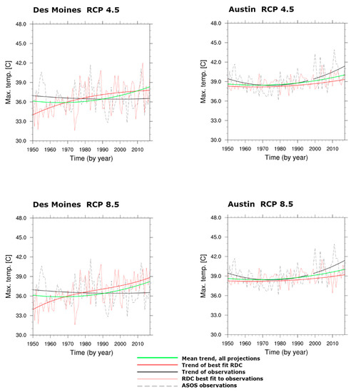
Figure 3.
Trend of annual maximum temperatures (black solid line) for Des Moines (left) and Austin (right) based on 67-years (1950–2017) historical observations compared to RDC data for RCP 4.5 (top) and RCP 8.5 (bottom) climate scenarios. Data and trends are identified by color and line type as given in the legend.
The trend in observed annual maximum temperature for Austin is different from that for Des Moines (Figure 3), with an increase of 3 °C between years 1980 through 2017, which is higher than the 1 °C increase in the mean temperature trend across the 42 (and 41) RDC forecasts of RCP 4.5 (and RCP 8.5) ensembles over the same period. The hottest extreme heat event of the “best fit” RDC forecast is more than 3 °C cooler than the hottest observed temperature for Austin, which occurred in 2011.
In general, the RDC annual maximum temperatures for Austin are cooler for most years than what has been observed, possibly suggesting an inability of GCMs to account sufficiently for the urban island heat effect and changes in urbanization due to their relatively coarse spatial resolution [13,14,15]. The GCMs that generated these RDC data do not invoke an urban canopy model, which is an option incorporated in certain regional models [41,42].
The opposing trends observed in both cities, Des Moines and Austin, between RDC temperature projections and observations since 1950 present a challenge in defining the most likely scenario for future heat extreme events using RDC data alone. Using both RDC forecasts and observations, a statistical approach is used here to define most likely future extreme temperatures based on the EMOS method as introduced in Section 2., and details of which are described in subsequent sections. Note that this projection of extreme temperatures using this statistical model is not to be interpreted as a specific forecast for a given point in time, but it aims to provide a statistical assessment of a reasonable range of future observations (within a 95% PI) by mid-century.
3.2. Constructing a Reduced-Order EMOS Model for Des Moines and Austin
The dataset of annual extreme temperatures from 1950 to 2017 is divided into training and testing periods. The training period is used for selecting the most influential covariates for each M-covariate reduced-order EMOS model while the testing period is used for model evaluation and model order selection. When the data size is limited, the training data can typically consist of, say, 70%–90% of the samples from the whole dataset (here 67 years, from 1950 to 2017) for capturing important trends and changes in historical data [43]. Accordingly, we consider three different training periods (with data up to 1997, 2002, and 2010) and associated testing periods (from 1998, 2003 and 2011, respectively, and all ending in 2017), which correspond to around 70%, 80%, and 90% training periods. In all three cases, we obtain fairly consistent prediction results; thus, we include here only results with the second combination, namely, data from 1950 to 2002 for the training period while the remaining data from 2003 to 2017 comprise the testing period. We omit results from other combinations in the interest of brevity.
We apply the greedy procedure combined with LOOCV, discussed in Section 2, to data from the training period, 1950 to 2002, for deciding on the covariates (or RDC projections) to be included in each -covariate model. Then, to decide on the final M, ideally we should choose a model with the lowest MSE and CRPS and highest PICP. However, a single fixed value of does not satisfy all three criteria. We note that four and five covariates, respectively, provide relatively low MSE and CRPS and high PICP values for Des Moines and Austin in the LOOCV. Therefore, we use M = 4 and 5 in our reduced-order model for predicting the annual peak temperature in Des Moines and Austin for the testing period.
Our analysis demonstrates that the reduced EMOS model can significantly improve prediction results over the full model that uses all RDC projections as covariates. For Des Moines, the MSE values over the testing period from the reduced model are 5.50 and 6.13, for RCP 4.5 and 8.5, respectively, whereas for Austin, these corresponding values are 4.08 and 3.87. In contrast, the MSE values from the full model are 13.97 (RCP 4.5) and 12.56 (RCP 8.5) for Des Moines and 13.84 (RCP 4.5) and 8.66 (RCP 8.5) for Austin. In effect, the reduced model leads to a reduction in MSE by 51%~71%. We also see substantial improvement in CRPS and PICP values. In the regression analysis, predictors are used as deterministic factors, so we do not make any assumptions on the distribution of the predictors. To validate the normality assumption, we perform the normality test with residuals (the difference between annual peak temperature and its predicted value) using a Kolmogorov–Smirnov test, the results of which support the normality assumption in most cases (not shown).
We note that the EMOS model prediction for Austin is more accurate than that for Des Moines. As discussed earlier, in addition to climate change, the cropland intensification in Des Moines has a substantial influence on the temperature in Des Moines. The current statistical model does not account for such factors and thus exhibits a larger deviation from observations in Des Moines compared to Austin. We plan to substantiate the combined effects of the regional warming hole and localized urban heating in a future study.
3.3. Determining Most Likely Range of Future Annual Peak Temperatures
Figure 4 compares prediction results from the reduced-order EMOS model with observed temperatures for Des Moines and Austin under the RCP 4.5 and 8.5 scenarios. The shaded band represents the 95% PI. The predicted highest temperatures (red line in Figure 4) from the statistical model are seen to generally be lower than what was observed (blue line) and predicted lowest temperatures are seen to be higher than what has been observed. This is because the model prediction makes use of a weighted linear combination of covariates, which tends to reduce data extremes. The PI, however, is proportional to the variance of the covariate data and can be interpreted as an envelope of likely values for the annual peak temperature. We note that the 95% PI includes most observational data points. Depending on the chosen climate scenario, RCP 4.5 or 8.5, it is projected that future annual peak temperatures will likely fall within the 95% PIs, as predicted annually out to 2040 in Figure 4 for Austin and Des Moines.
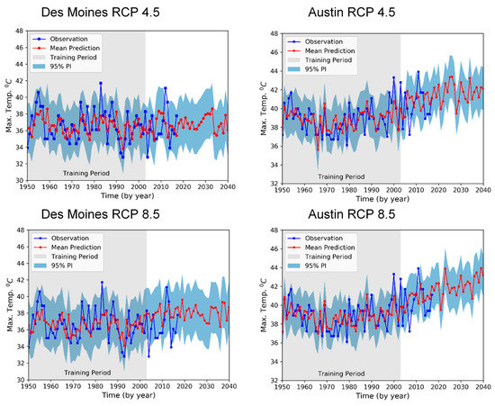
Figure 4.
Annual mean peak temperature predictions (red lines) with envelope for 95% PI (aqua) and observed annual maximums (blue lines) from 1950 to 2017 for Des Moines and Austin. Predicted values are based on RDC projections of RCP 4.5 (top) and 8.5 (bottom) climate scenarios.
Overall, the 95% PI for Des Moines is predicted to remain nearly the same as present values out to 2040 for both the RCP 4.5 and 8.5 climate scenarios, albeit with relatively strong year-to-year variations in the period around 2030. For Austin, there is a predicted increase in annual extreme temperatures (Figure 4). The Austin 95% PI median value for RCP 4.5 increases by roughly 1 °C between the mid-2010′s and the mid-2020′s, but levels out thereafter through 2040 (Figure 4). The Austin 95% PI median value for RCP 8.5 increases by roughly 2 °C between the mid-2010′s through 2040.
Figure 5 compares observed temperatures with predicted temperatures from the reduced-order EMOS model (see the mean prediction trajectories) and with the RDC projections included in the reduced-order EMOS model (see the gray trajectories). Although the RDC models project increasing temperatures in the future in Des Moines (Figure 5, left panel), the reduced-order EMOS model diverges from these RDC projections, resulting in future heat extremes that are lower than those of the RDC projections. This discrepancy may be caused by increased evapotranspiration linked to crop intensification in the Midwest, an effect not well represented by the RDC projections but considered in the reduced-order EMOS model prediction of annual extreme temperatures.
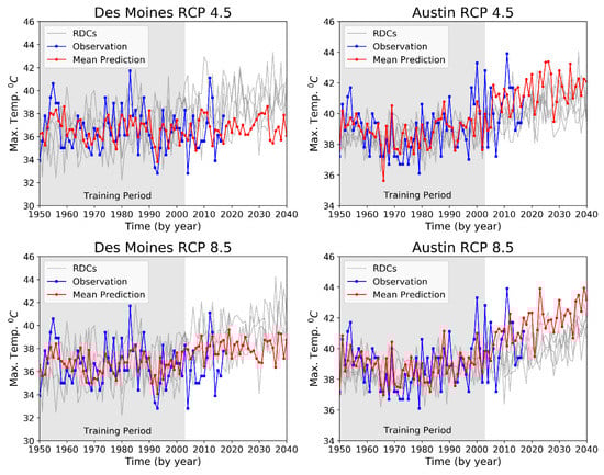
Figure 5.
Annual maximum temperature observations (blue lines with square markers), predictions from the reduced-order EMOS model (red lines with circle markers) and RDC projections (gray lines) for Des Moines and Austin.
On the contrary, the right panel of Figure 5 shows that in Austin, the reduced-order EMOS model annual peak temperature predictions are slightly higher than those from the suite of RDC projections. RDC data do not sufficiently account for the impact of localized warm areas due to urban heat islands in densely populated city environments such as Austin. By incorporating observations along with RDC data, the statistical model is able to account for such local urban heat island effects.
4. Discussion and Conclusions
Using the EMOS method, the likely range (95% PI) of future extreme high temperatures is found for Austin to trend higher by 1–2 °C by 2040, but to remain nearly the same for Des Moines. These EMOS model results do not identically align with RDC projections. For Austin, the RDC data likely do not effectively account for the heat island effect for large and densely populated areas; this causes RDC extreme temperature projections to be slightly lower than those with the EMOS method, which takes into account observational data along with RDC projections to formulate future extreme temperature projections. For Des Moines, the RDC projections are warmer compared to those from the EMOS model. Cropland intensification in the Midwest has been influential in preventing an increase in temperature extremes over the past decades, a factor that is not accounted for in the RDC projections but is implicitly included in the EMOS model as long as such effect, even if non-linear, is of sufficient consequence as to influence temperature solutions during the training period. The relatively wide 95% PI for Des Moines, compared to that for Austin, suggests greater prediction uncertainty for Des Moines climate projections, which is possibly dependent on a change in crop production as well as future precipitation that allows continued substantial evapotranspiration and has an impact on whether or not such a warming hole persists in the Midwest.
The results of the present study not only suggest that a careful comparison should be made between observation trends and climate model trends to account for regional differences in the fidelity of the climate models when estimating future impacts of climate change on energy needs in specified locations, but that the same care should be exercised when considering changes in other weather and land parameters. For example, modeled regional changes in precipitation and agricultural practices must be considered in order to account for the Midwest warming hole as well as changes in urban population density that will modify the urban heat island effect. Moreover, changes in regional characteristics in the future, such as increasing urbanization, growing urban population, and different land use, will affect future extreme heat events. This study does not account for such changes, as we assume a similar trend exhibited in 1950–2017 will continue until mid-century. In the future, we plan to investigate the influence of the changes in regional characteristics on the urban extreme temperatures.
Predictions of the occurrence of extreme heat events in large cities, such as through the use of the models and methods developed in this work, are of great importance in a wide range of applications and, in particular, for electric grid resource planning. Given that electricity demand and production are highly dependent on ambient temperatures, there are periods where the highest peak temperatures occur that cause stress for an electric grid, increasing electricity prices, and grid congestion, with a reduced reserve margin. Thus, for a utility company or municipality, the findings from this work of the importance of localized considerations for extreme event predictions help point to a need for further in-depth analysis of such predictions. This will help to set aside necessary investments to balance generation and consumption and to ensure sufficient capacity of transmission and distribution to maintain grid reliability. Thus, the results of this work can be utilized for regional planning purposes. They also motivate the need for further work to integrate weather predictions with localized condition considerations such as urban heat island effects.
Author Contributions
Conceptualization, D.E.J., W.A.G.J., K.C., E.B., L.M., and Y.Z.; methodology, D.E.J., W.A.G.J., P.T.T.N., E.B., L.M., K.C., Q.P., and E.J.; software, D.E.J., P.T.T.N., and Q.P.; formal analysis, D.E.J., W.A.G.J., P.T.T.N., E.B., L.M., K.C., Q.P., and E.J.; writing—original draft preparation, D.E.J., P.T.T.N., E.B., and K.C.; writing—review and editing, D.E.J., P.T.T.N., E.B., K.C., W.A.G.J., and L.M.; visualization, D.E.J., P.T.T.N., and Q.P.; supervision, D.E.J., K.C., E.B., and L.M.; project administration, K.C., W.A.G.J., and D.E.J.; funding acquisition, K.C. and W.A.G.J.
Funding
This material is based upon work supported by the U.S. National Science Foundation under Grant Nos. CMMI-1662691, CMMI-1663044, and CMMI-1662553. Any opinions, findings, and conclusions or recommendations expressed in this material are those of the authors and do not necessarily reflect the views of the National Science Foundation.
Acknowledgments
We acknowledge the World Climate Research Program’s Working Group on Coupled Modelling, which is responsible for CMIP, and we thank the climate modeling groups (listed in Table 1 of this paper) for producing and making available their model output. For CMIP, the U.S. Department of Energy’s Program for Climate Model Diagnosis and Intercomparison provides coordinating support and led development of software infrastructure in partnership with the Global Organization for Earth System Science Portals. Also, we acknowledge the insightful comments of the reviewers, which helped us to improve the manuscript.
Conflicts of Interest
The authors declare no conflict of interest.
Appendix A
Formulation of the Reduced-Order EMOS Model
First, for quantifying prediction uncertainty, we note that the assessment of probabilistic models should consider the reliability and the sharpness of predictive output density. Accordingly, to measure first the reliability, we use the PICP which is the percentage of observations that fall within the PI, defined as
where and denote upper and lower bounds of the PI corresponding to the th data point in the studied period, and if ; otherwise, . Ideally, it is expected that the value of the should be close to 95%, and the model is not reliable if is much less than 95%.
When the PI is wide, the desired 95% coverage value for the metric of can be easily satisfied. A wide PI, however, implies large prediction uncertainty and it conveys little information for predictions. Therefore, secondarily, we may also consider the average width of PIs which can quantify the sharpness of the predictive density [44,45]. A narrower PI implies a sharper forecast, asserting that the uncertainty in the predictions is concentrated and lower; the prediction is thus more valuable.
Although it would be ideal to obtain a narrow PI with a high coverage probability, theoretically these two criteria work against each other. The CRPS combines these two metrics into a single criterion that is useful for comparing different models when the aim of the probabilistic forecasting is to maximize the sharpness of the predictive distribution under proper reliability [25]. The CRPS of a normal distribution is defined as
where and denote the probability density function (PDF) and the cumulative distribution function (CDF), respectively, of a standard normal random variable. We use the average CRPS score as:
Once -covariate models, , for RCP 4.5 (RCP 8.5) are selected using the aforementioned greedy procedure, we collectively evaluate their MSEs, 95% PICPs and CRPS and choose the model that best minimizes MSE and CRPS while also maximizing coverage probability.
References
- Koppe, C.; Kovats, S.; Jendritzky, G.; Menne, B. Heat-Waves: Risks and Responses. In WHO Report: Health and Global Environmental Change Series; No. 2; WHO: Geneva, Switzerland, 2004; p. 123. ISBN 92-890-1094-0. [Google Scholar]
- Harmon, K. How Does a Heat Wave Affect the Human Body? Scientific American, 2010. Available online: https://www.scientificamerican.com/article/heat-wave-health (accessed on 19 April 2018).
- U.S. Department of Energy. Energy Information Administration Retail Use of Electricity, Annual, Independent Statistics & Analysis. 2017. Available online: https://www.eia.gov/electricity/data.php (accessed on 20 March 2018).
- U.S. Department of Energy. Energy Information Administration, Residential Consumption Survey. Independent Statistics & Analysis. 2015. Available online: https://www.eia.gov/consumption/residential/data/2015/hc/php/hc7.6.php (accessed on 20 March 2018).
- Añel, J.A.; Fernández-González, M.; Labandeira, X.; López-Otero, X.; de la Torre, L. Impact of cold waves and heat waves on the energy production sector. Atmosphere 2017, 8, 209. [Google Scholar] [CrossRef]
- Rademaekers, K.; van der Laan, J.; Boeve, S.; Lise, W.; van Hienen, J.; Metz, B.; Haigh, P.; de Groot, K.; Dijkstra, S.; Jansen, J. Investment Needs for Future Adaptation Measures in EU Nuclear Power Plants and Other Electricity Generation Technologies due to Effects of Climate Change; Technical Report; European Commission: Brussels, Belgium, 2011. [Google Scholar]
- Global Climate Change Impacts in the United States. United States Global Change Research Program; Thomas, R.K., Melillo, J.M., Peterson, T.C., Eds.; Cambridge University Press: New York, NY, USA, 2009.
- U.S. Global Change Research Program. Climate Science Special Report: Fourth National Climate Assessment; Wuebbles, D.J., Fahey, D.W., Hibbard, K.A., Dokken, D.J., Steward, B.C., Maycock., T.K., Eds.; U.S. Global Change Research Program: Washington, DC, USA, 2017; p. 470. [CrossRef]
- Collins, M.; Knutti, R.; Arblaster, J.; Dufresne, J.-L.; Fichefet, T.; Friedlingstein, P.; Gao, X.; Gutowski, W.J.; Johns, T.; Krinner, G.; et al. Long-term Climate Change: Projections, Commitments and Irreversibility. In Climate Change 2013: The Physical Science Basis; Contribution of Working Group I to the Fifth Assessment Report of the Intergovernmental Panel on Climate Change; Stocker, T.F., Qin, D., Plattner, G.-K., Tignor, M., Allen, S.K., Boschung, J., Nauels, A., Xia, Y., Bex, V., Midgley, P.M., Eds.; Cambridge University Press: Cambridge, UK; New York, NY, USA, 2013. [Google Scholar]
- Pachauri, R.K.; Meyer, L.A. (Eds.) Climate Change 2014: Synthesis Report. In Contribution of Working Groups I, II and III to the Fifth Assessment Report of the Intergovernmental Panel on Climate Change; IPCC: Geneva, Switzerland, 2014; p. 151. [Google Scholar]
- Pryor, S.C.; Scavia, D.; Downer, C.; Gaden, M.; Iverson, L.; Nordstrom, R. Climate Change Impacts in the United States: The Third National Climate Assessment. In National Climate Assessment Report; Melillo, J.M., Richmond, T.C., Yohe, G.W., Eds.; U.S. Global Change Research Program: Washington, DC, USA, 2014. [Google Scholar]
- Oke, T.R. City size and the urban heat island. Atmos. Environ. 1967, 7, 769–779. [Google Scholar] [CrossRef]
- Oke, T.R. The energetic basis of the Urban Heat Island. Q. J. R. Meteorol. Soc. 1982, 108, 1–24. [Google Scholar] [CrossRef]
- Arnfield, A.J. Two decades of urban climate research: A review of turbulence, exchanges of energy and water, and the urban heat island. Int. J. Climatol. 2003, 23, 1–26. [Google Scholar] [CrossRef]
- Quattrochi, D.A.; Luvall, J.C.; Rickman, D.L.; Estes, M.G.; Laymon, C.A.; Howell, B.F. A decision support information system for urban landscape management using thermal infrared data: Decision support systems. Photogramm. Eng. Remote Sens. 2000, 66, 1195–1207. [Google Scholar]
- Pan, Z.; Arritt, R.W.; Takle, E.S.; Gutowski, W.J., Jr.; Anderson, C.J.; Segal, M. Altered hydrologic feedback in a warming climate introduces a “warming hole”. Geophys. Res. Lett. 2004, 31, L17109. [Google Scholar] [CrossRef]
- Sillmann, J.; Kharin, V.V.; Zhang, X.; Zwiers, F.W.; Bronaugh, D. Climate extremes indices in the CMIP5 multimodel ensemble: Part 1. Model evaluation in the present climate. J. Geophys. Res. 2013, 118, 1716–1733. [Google Scholar] [CrossRef]
- Meehl, G.A.; Arblaster, J.M.; Branstator, G. Mechanisms Contributing to the Warming Hole and the Consequent U.S. East–West Differential of Heat Extremes. J. Clim. 2012, 25, 6394–6408. [Google Scholar] [CrossRef]
- Mascioli, N.R.; Previdi, M.; Fiore, A.M.; Ting, M.F. Timing and seasonality of the United States ‘warming hole’. Environ. Res. Lett. 2017, 12, 034008. [Google Scholar] [CrossRef]
- Mueller, N.D.; Butler, E.E.; McKinnon, K.A.; Rhines, A.; Tingley, M.; Holbrook, N.M.; Huybers, P. Cooling of US Midwest summer temperature extremes from cropland intensification. Nat. Clim. Chang. 2015, 6, 317–324. [Google Scholar] [CrossRef]
- Hurrell, J.; Visbeck, M.; Pirani, A. WCRP Coupled Model Intercomparison Project—Phase 5: Special Issue of the CLIVAR Exchanges Newsletter; No. 56, 15, No. 2; CLIVAR Exchanges: Qingdao, China, 2011. [Google Scholar]
- Taylor, K.E.; Stouffer, R.J.; Meehl, G.A. An Overview of CMIP5 and the experiment design. Bull. Am. Meteorol. Soc. 2012, 93, 485–498. [Google Scholar] [CrossRef]
- Maurer, E.P.; Brekke, L.; Pruitt, T.; Duffy, P.B. Fine-resolution climate projections enhance regional climate change impact studies. Eos Trans. 2007, 88, 504. [Google Scholar] [CrossRef]
- Brekke, L.; Thrasher, B.L.; Maurer, E.P.; Pruitt, T. Downscaled CMIP3 and CMIP5 Climate and Hydrology Projections: Release of Downscaled CMIP5 Climate Projections, Comparison with Preceding Information, and Summary of User Needs; The U.S. Department of the Interior, Bureau of Reclamation, Technical Services Center: Denver, CO, USA, 2013; p. 47.
- Gneiting, T.; Raftery, A.E.; Westveld, A.H.; Goldman, T. Calibrated probabilistic forecasting using ensemble model output statistics and minimum CRPS estimation. Mon. Weather Rev. 2005, 133, 1098–1118. [Google Scholar] [CrossRef]
- United States Census Bureau. Annual Estimates of the Resident Population for Incorporated Places of 50,000 or More, Ranked by July 1, 2018 Population: April 1, 2010 to July 1, 2018. Available online: https://factfinder.census.gov/faces/tableservices/jsf/pages/productview.xhtml?src=bkmk (accessed on 8 November 2019).
- United States Census Bureau. 2016 U.S. Gazetteer Files. Available online: https://www2.census.gov/geo/docs/mapsdata/data/gazetteer/2016_Gazetteer/2016_Gaz_tracts_national.zip (accessed on 8 November 2019).
- U.S. Climate Data. Available online: http://usclimatedata.com (accessed on 8 November 2019).
- Doyle, A. Global Warming Set to Exceed 1.5 °C, Slow Growth—U.N. Draft. Environment. Available online: https://www.reuters.com/article/us-climatechange-report-exclusive/exclusive-global-warming-set-to-exceed-1-5c-slow-growth-u-n-draft-idUSKBN1JA1HD (accessed on 24 August 2018).
- Iowa State University, Iowa Environmental Mesonet: ASOS Network Historical Data. Available online: https://mesonet.agron.iastate.edu/ASOS (accessed on 20 September 2017).
- Van Vuuren, D.P.; Edmonds, J.; Kainuma, M.; Riahi, K.; Thomson, A.; Hibbard, K.; Hurtt, G.C.; Kram, T.; Krey, V.; Lamarque, J.-F.; et al. The representative concentration pathways: An overview. Clim. Chang. 2011, 109, 5–31. [Google Scholar] [CrossRef]
- Thorarinsdottir, T.L.; Gneiting, T. Probabilistic forecasts of wind speed: Ensemble model output statistics by using heteroscedastic censored regression. J. R. Stat. Soc. 2010, 173, 371–388. [Google Scholar] [CrossRef]
- Friederichs, P.; Thorarinsdottir, T.L. Forecast verification for extreme value distributions with an application to probabilistic peak wind prediction. Environmetrics 2012, 23, 579–594. [Google Scholar] [CrossRef]
- Baran, S.; Lerch, S. Log-normal distribution based Ensemble Model Output Statistics models for probabilistic wind-speed forecasting. Q. J. R. Meteorol. Soc. 2015, 141, 2289–2299. [Google Scholar] [CrossRef]
- Baran, S.; Lerch, S. Mixture EMOS model for calibrating ensemble forecasts of wind speed. Environmetrics 2016, 27, 116–130. [Google Scholar] [CrossRef]
- Friedman, J.; Hastie, T.; Tibshirani, R. The Elements of Statistical Learning: Data Mining, Inference, and Prediction, 2nd ed.; Springer Series in Statistics; Springer: New York, NY, USA, 2009; p. 737. [Google Scholar]
- Hoerl, A.; Kennard, R. Ridge regression. Encycl. Stat. Sci. 1988, 8, 129–136. [Google Scholar]
- Tibshirani, R. Regression shrinkage and selection via the lasso. J. R. Stat. Soc. B 1996, 58, 267–288. [Google Scholar] [CrossRef]
- Goeman, J.; Meijer, R.; Chaturvedi, N. L1 and L2 Penalized Regression Models: Documentation for the Penalized Package for the Statistical Environment R. Available online: https://cran.r-project.org/web/packages/penalized/vignettes/penalized.pdf (accessed on 15 November 2018).
- Byon, E.; Shrivastava, A.K.; Ding, Y. A classification procedure for highly imbalanced class sizes. IIE Trans. 2010, 42, 288–303. [Google Scholar] [CrossRef]
- Kusaka, H.; Kondo, H.; Kikegawa, Y.; Kimura, F. A simple single-layer urban canopy model for atmospheric models: Comparison with multi-layer and slab models. Bound. Layer Meteorol. 2001, 101, 329–358. [Google Scholar] [CrossRef]
- Kusaka, H.; Kimura, F. Coupling a single-layer urban canopy model with a simple atmospheric model: Impact on urban heat island simulation for an idealized case. J. Meteorol. Soc. Jpn. 2004, 82, 67–80. [Google Scholar] [CrossRef]
- Lee, G.; Byon, E.; Ntaimo, L.; Ding, Y. Bayesian spline method for assessing extreme loads on wind turbines. Ann. Appl. Stat. 2013, 7, 2034–2061. [Google Scholar] [CrossRef]
- Khosravi, A.; Nahavandi, S.; Creighton, D.; Atiya, A.F. Lower upper bound estimation method for construction of neural network-based prediction intervals. IEEE Trans. Neural Netw. 2011, 22, 337–346. [Google Scholar] [CrossRef] [PubMed]
- Shrestha, D.L.; Solomatine, D.P. Machine learning approaches for estimation of prediction interval for the model output. Neural Netw. 2006, 19, 225–235. [Google Scholar] [CrossRef]
© 2019 by the authors. Licensee MDPI, Basel, Switzerland. This article is an open access article distributed under the terms and conditions of the Creative Commons Attribution (CC BY) license (http://creativecommons.org/licenses/by/4.0/).