Comparison of PM_2.5 Chemical Components over East Asia Simulated by the WRF-Chem and WRF/CMAQ Models: On the Models’ Prediction Inconsistency

Abstract

High levels of atmospheric concentration of PM_2.5 (particulate matters less than 2.5 μm in size) are one of the most urgent societal issues over the East Asian countries. Air quality models have been used as an essential tool to predict spatial and temporal distribution of the PM_2.5 and to support relevant policy making. This study aims to investigate the performance of high-fidelity air quality models in simulating surface PM_2.5 chemical composition over the East Asia region in terms of a prediction consistency, which is a prerequisite for accurate air quality forecasts and reliable policy decision. The WRF-Chem (Weather Research and Forecasting-Chemistry) and WRF/CMAQ (Weather Research and Forecasting/Community Multiscale Air Quality modeling system) models were selected and uniquely configured for a one-month simulation by controlling surface emissions and meteorological processes (model options) to investigate the prediction consistency focusing the analyses on the effects of meteorological and chemical processes. The results showed that the surface PM_2.5 chemical components simulated by both the models had significant inconsistencies over East Asia ranging fractional differences of 53% ± 30% despite the differences in emissions and meteorological fields were minimal. The models’ large inconsistencies in the surface PM_2.5 concentration were attributed to the significant differences in each model’s chemical responses to the meteorological variables, which were identified from the multiple linear regression analyses. Our findings suggest that the significant models’ prediction inconsistencies should be considered with a great caution in the PM_2.5 forecasts and policy support over the East Asian region.

1. Introduction

Public concerns have been explosively increased over the East Asian countries since atmospheric particulate matters with an aerodynamic diameter less than 2.5 μm (PM_2.5) had been classified as a first-grade carcinogen risk by the World Health Organization (WHO) in 2013 [1]. Many studies have reported adverse impacts of PM_2.5 on human health (e.g., [2,3,4,5,6,7,8]). For example, Laden et al. [9] showed that the PM_2.5 enhancement of 10 μg m⁻³ from motor vehicle exhaust increased the daily mortality rate by 3.4% in six cities of the United States (U.S.). Ostro et al. [2] demonstrated statistical associations between PM_2.5 and daily mortality in nine California counties in U.S. Many studies based on a time-series analysis suggested that specific PM_2.5 chemical components have higher correlations with daily mortality than the total PM_2.5 mass concentration, showing the statistical relations between the PM_2.5 chemical components of sulfates, element carbon, and organic carbon with cardiovascular deaths (e.g., [3,4]). Besides, the atmospheric PM_2.5 have been known to have significant influences on ecosystems, visibility, and meteorological and climatological changes (e.g., [10]).

Air quality models (AQMs) predict spatial and temporal variations of the PM_2.5 chemical composition over the area of interest, which have been developed as an essential tool for air quality forecasts, health and environmental impact assessments, and policy support [11,12,13]. The Community Multiple Air Quality (CMAQ) model [14,15] and the Weather Research and Forecast-Chemistry (WRF-Chem) model [16] have been frequently used to study local/regional scale air quality problems (e.g., [17,18,19,20,21]). Appel et al. [22] applied the CMAQ model to simulate the PM_2.5 concentration over the U.S. and the Europe, and found that the simulated PM_2.5 concentration was underestimated by 45–65% against measurements. Zhang et al. [23] conducted a 7-year long-term simulation for the eastern U.S. using the CMAQ model and showed a significant underestimation of organic carbon (OC) but a reasonable performance in nitrates (NO₃⁻) and sulfates (SO₄²⁻). Lang et al. [24] used the CMAQ model to simulate the PM_2.5 chemical composition in Beijing, China and suggested to reduce secondary inorganic aerosols (SIA) for improvement of the air quality due to their high fraction of more than 50% in the PM_2.5 concentration. Qin et al. [25] studied characteristics of the PM_2.5 chemical composition in the Pearl River Delta region, China using the CMAQ model and showed the model tended to underestimate total PM_2.5 and OC concentrations by 21–28% and approximately 59% against measurements, respectively. Song et al. [26] evaluated the performance of the CMAQ model in simulating the PM_2.5 chemical components over East Asia and showed the underestimation in sulfates but the overestimation in nitrates for most of the simulation domain, being attributed to inaccurate SO₂ aqueous chemical reaction. Zhou et al. [27] evaluated the performance of the WRF-Chem model in PM_2.5 forecasts over the eastern China and found that the daily average PM_2.5 concentration was underestimated by approximately 13% on average. In general, the AQMs underestimated SO₄²⁻ and OC but overestimated NO₃⁻, overall resulting in underestimation of total PM_2.5 concentration. In most previous studies, a single AQM was used and the model’s performance was evaluated against measurements at different time and space before their applications.

Some studies have compared the performance between the two models in simulating the PM_2.5 chemical composition [28,29,30,31,32,33]. Matsui et al. [28] examined the spatial and temporal variations of PM_2.5 around Beijing in summer 2006 using the WRF/CMAQ model. In the study, the performance of the WRF-Chem model was also compared against intensive field measurements with the WRF/CMAQ model. The results showed that the WRF-Chem model simulated primary aerosol species (e.g., EC) higher by approximately 20% than the WRF/CMAQ in Beijing, attributing to the lower vertical mixing in the WRF-Chem model. The model discrepancy was reduced by less than 10–20% in secondary inorganic components (e.g., SO₄²⁻, NO₃⁻, NH₄⁺) due to chemical production within the atmospheric boundary layer. Zhang et al. [32] compared the performances of the WRF-Chem model and the MM5/CMAQ model for the East Asian domain against meteorological and chemical measurements for one year of 2006. The MM5/CMAQ model performed better than the WRF-Chem model in simulating the meteorological variables of 2-m temperature and 10-m wind speed in South Korea and Japan, while both the models underestimated the PM_2.5 concentration ranging from approximately −25% to −74% against surface measurements in Taiwan. Though the models’ performances in simulating PM_2.5 chemical components at different geographic locations and times have been statistically evaluated through comparison with available chemical measurements, overall, characteristic differences between the models have not been carefully considered.

The purpose of this study is to investigate the performance of high-fidelity AQMs of WRF-Chem and WRF/CMAQ in simulating surface PM_2.5 chemical components over the East Asian region focusing on the models’ prediction consistency. The surface PM_2.5 chemical components were analyzed because that plays a key role in air quality forecasts and policy making. A better understanding of the models’ relative consistency between the models is prerequisite for more accurate forecasts and reliable policy decision supports. In this study, large model-model inconsistencies in mass concentrations of the PM_2.5 chemical components over East Asia were identified, and the causes of the inconsistencies had been investigated in association with meteorological influences on the chemical processes of the models. The remainder of the manuscript is structured as follows: Section 2 describes the selected air quality models and an experimental design to identify the models’ prediction inconsistency and possible causes to explain the relative inconsistencies. Section 3 compares first the PM_2.5 chemical components over East Asia simulated by the WRF-Chem and WRF/CMAQ models along with validation of the simulated meteorological fields against measurements. Then, the meteorological influences on the models’ inconsistencies in the simulated PM_2.5 chemical components are examined. Summary and conclusions follow in Section 4.

2. Methods

2.1. Air Quality Models: WRF-Chem and WRF/CMAQ

The regional scale AQMs of WRF-Chem [16] and WRF/CMAQ [15] were used to simulate and compare the surface PM_2.5 chemical components over East Asia. First, the WRF model is a three-dimensional Eulerian meteorological model that solves a set of prognostic conservation equations for mass, momentum, energy, and moisture and associated atmospheric physical processes such as short- and long-wave radiative transfer, atmospheric boundary layer turbulent mixing, surface-atmosphere interactions, and precipitation [34]. The WRF-Chem model is an ‘on-line’ 3-dimensional Eulerian air quality model that calculates anthropogenic and biogenic emissions processes, chemical transport and transformation processes, dry and wet depositions of gaseous and aerosol species on an interactive mode with the WRF model. Since the model integrates the meteorological and chemical processes simultaneously at a model’s integration time step, it is capable of realistically representing complex physical and chemical interactions occurred in the atmosphere. Meanwhile, the CMAQ model is another 3-dimensional Eulerian air quality model that has been developed primarily for regional air quality forecasts by the U.S. Environmental Protection Agency (EPA). It calculates the meteorological and chemical processes for atmospheric evolution of the gaseous and aerosol species. However, meteorological fields are independently prepared first by the WRF model, and then they are fed to the CMAQ model through a Meteorology-Chemistry Interface Processor (MCIP) package to calculate the chemical processes (‘WRF/CMAQ’). Unlike the WRF-Chem model, the WRF/CMAQ model is an ‘offline’ air quality model that computes the meteorological and chemical fields sequentially [31]. Both the air quality models have been widely applied in air quality forecasts (e.g., [27,35]), top-down emission verification (e.g., [36,37]), regulatory suggestion (e.g., [24]), and scientific problems (e.g., [38,39,40,41,42,43]).

2.2. Experimental Setup

The WRF-Chem and WRF/CMAQ models were uniquely configured to simulate the PM_2.5 chemical components over the East Asia region and to examine characteristic features in terms of the models’ prediction consistency. Both the meteorological options and the anthropogenic/biogenic emissions were assigned identically except for cumulus parameterization, while the chemical processes (e.g., gaseous and aerosols chemistry, dry and wet depositions) were used their own options. These model configurations can reduce the diversity of the models’ performance from direct meteorological effects (e.g., transport, turbulent mixing) as well as emission processes. The meteorological influences on the simulations of PM_2.5 chemical components may be largely attributed to the physical integration mode, that is, ‘on-line’ and ‘off-line’.

2.2.1. Model Configuration

The spatial domains of the WRF-Chem (ver. 3.6) and WRF/CMAQ (ver. 3.4.1/ver. 4.7.1) models cover identically a large East Asian region including China, Korea, and Japan (Figure 1). The horizontal grid resolution was set by 30 km (190 × 135 mesh) and the vertical grid was irregularly configured stretching from ~15 m above ground level at the lowest grid to ~20 km (50 hPa) at the domain top. The 18 lower vertical layers are below 2000 m to better represent the physical chemical processes within the planetary boundary layer (PBL). The WRF-Chem model simulated the meteorological fields and the chemical concentration fields at the same 43 sigma levels, while the CMAQ model calculated the chemical concentration fields at 23 reduced sigma levels, for which the MCIP produced the meteorological fields compatible to the CMAQ grid from the WRF-predicted meteorological fields at 43 sigma levels. The use of reduced vertical grid resolution in the WRF/CMAQ model was frequently selected for a computational efficiency (e.g., [44])

The meteorological physics options were configured identically for both the models except for cumulus parametrization: the Dudhia scheme [45] and RRTMG [46] for shortwave and longwave radiation, the YSU scheme [47] for PBL turbulence mixing, the NoahLSM [48] for surface-atmosphere interactions, and the WSM3 scheme [49] for grid-scale microphysics. For cumulus parameterization, the WRF-Chem and WRF/CMAQ models used the Grell-Freitas scheme [50] and the Kain-Fritsch scheme [51], respectively. Since none of them were available for both the models, the sub-grid cloud physics were set differently in the models. Meanwhile, chemical gaseous and aerosol mechanisms were configured with their own mechanisms. The WRF-Chem used the Regional Atmospheric Chemistry Mechanism (RACM) [52] and the Modal Aerosol Dynamics model for Europe/Secondary ORGanic Aerosol Model (MADE/SORGAM) [53,54] for gaseous and aerosol chemistry, respectively. Meanwhile, the WRF/CMAQ used the Statewide Air Pollution Research Center, version 99 (SAPRC-99) [55] and the aerosol module version 5 (AERO5) [56]. The SAPRC-99 includes 93 chemical species and 213 reactions and the AERO5 module represents sizable aerosols by three functional distributions of Aitken (less than 0.1 μm), accumulation (0.1–2 μm), and coarse (2 μm or larger) modes. Aerosol dynamics of nucleation, condensational growth, and coagulation are considered with the gas-phase and heterogeneous aqueous chemistry. The gaseous and heterogeneous chemistry mechanisms used in both the models treat elemental carbon (EC), primary organic aerosols (POA), secondary organic aerosols (SOA), and secondary inorganic aerosols (SIA) along with coarse particulate matters of soil dust, sea salt, and other non-reactive anthropogenic particulate matters. The SOA are primarily formed by homogeneous reaction between ozone (O₃), hydroxyl radicals (OH), oxygenated NO_x (NO₃) and organic compounds, and the POA are assumed to be non-volatile and inert primary emission components such as EC [57]. Overall, the meteorological and chemical options used for conducting the models are given in

Table 1. Configuration of the Weather Research and Forecasting-Chemistry (WRF-Chem) and Weather Research and Forecasting/Community Multiscale Air Quality modeling system (WRF/CMAQ) models.

	WRF-Chem	WRF/CMAQ
Horizontal grid	190 × 135 (ΔX = 30 km)	190 × 135 (ΔX = 30 km)
Vertical layer	43	43/23
Shortwave radiation	Dudhia [45]	Dudhia
Longwave radiation	RRTMG [46]	RRTMG
Turbulence	YSU [47]	YSU
Land-surface	Noah LSM [48]	Noah LSM
Microphysics	WSM3 [49]	WSM3
Cumulus parameterization	Grell-Freitas [50]	Kain-Fritsch [51]
Gas phase chemistry	RACM [52]	SAPRC−99 [55]
Aerosol mechanism	MADE/SORGAM [53,54]	AERO5 [56]

.

The simulations were conducted over the East Asian domain for a month period of April 2010, which is a base year of the anthropogenic emission inventories used in this study. The meteorological initial and boundary conditions were obtained from the National Centers for Environmental Prediction-Final Analysis (NCEP-FNL) that is a global reanalysis data with a spatial resolution of 1° × 1° and a temporal resolution of 6 hrs. The meteorological fields of 3-dimensional air temperature, specific humidity, and horizontal wind vector simulated by the WRF model were nudged to the corresponding large-scale meteorological fields using the 4-dimensional data assimilation (4DDA) technique during the whole simulation period [58]. Lee et al. [42] suggested to use approximately 56-days chemical spin-up time from the WRF-Chem simulation of a similar size East Asian domain. Thus, the analyses were primarily conducted with the simulation results of 24 days, discarding initial 6 days results for the models’ spin-up. The six sub-regions of the northern China (R1), central China (R2), southern China (R3), North Korea (R4), South Korea (R5), and Japan (R6) were defined to characterize the models’ relative performance at different geographical locations (Figure 1).

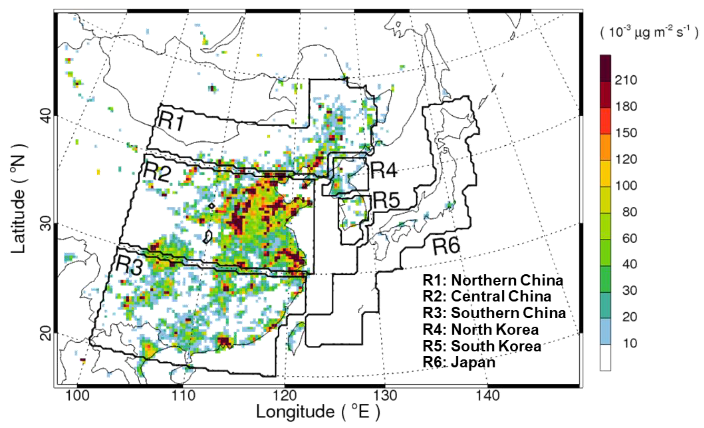
2.2.2. Anthropogenic and Biogenic Emissions

The anthropogenic emissions inventory that was developed for the Model Inter-Comparison Study for Asia 2010 (MICS-Asia 2010) [59,60] was used to process for gridded anthropogenic emissions. The inventory combined 29 Asian countries’ emission inventories primarily including the Regional Emission Inventory in Asia (REAS) [61], the Multi-resolution Emission Inventory China (MEIC) (http://www.meicmodel.org), the Japan Auto-Oil Program emission inventory (JATOP), and the Korean Clear Air Policy Support System (CAPSS) [62]. The emission chemical species in the MICS-Asia 2010 include black carbon (BC), carbon monoxide (CO), sulfur dioxide (SO₂), nitrogen oxides (NO_x), ammonia (NH₃), non-methane volatile organic compounds (VOCs), organic carbon (OC), and primary particulate matters of PM_2.5 and PM₁₀. The primary anthropogenic emission species were gridded compatible to the model using the Sparse Matrix Operator Kernel for Emissions (SMOKE) module [63]. The non-methane VOCs emissions were decomposed into the SAPRC−99 chemical species for the WRF/CMAQ model, which were then converted into the RACM chemical species for the WRF-Chem model using a chemical conversion table followed by Lee et al. [42]. The spatial distributions of the gridded anthropogenic emissions processed for the simulation in this study are presented in Figure 2. Strong continental emissions were clearly identified especially in the central and southern China (R2 and R3).

The biogenic VOCs emitted from the Earth’s terrestrial biosphere include hydrocarbons such as isoprene, monoterpenes, and sesquiterpenes as well as oxygenated organic compounds. The chemical species are highly reactive in the troposphere, leading to formation of CO, OH, and O₃ (e.g., [64]) as well as biogenic SOA (e.g., [65,66]). The emission fluxes of the biogenic VOCs change with meteorological and environmental conditions (e.g., temperature, radiation, ozone, carbon dioxide) [67,68,69] as well as vegetation species. This study used the Model of Emissions of Gases and Aerosols from Nature, version 2.04 (MEGAN-2) [70], which calculates 134 chemical species including isoprene, monoterpenes, sesquiterpenes, and other oxygenated VOCs by considering various vegetation species and time-varying environmental conditions. The biogenic emissions were calculated over the East Asian domain for the simulation period in an offline mode using the global land-cover dataset (1 km² resolution) and the meteorological conditions simulated by the WRF model. It is worthy to note that the WRF-Chem model has a capability to calculate the biogenic emissions at every time step during the model integration (‘online’). Here, the pre-calculated biogenic emissions were applied identically in both the models to control the emissions in the simulations.

2.3. Measurements

2.3.1. Meteorological Measurements

The five meteorological variables of 2-m temperature, 10-m wind speed, relative humidity, precipitation, and PBL height are generally considered as important meteorological controlling factors that can modulate the atmospheric concentrations (e.g., [71,72,73]). The three surface meteorological variables (2-m temperature, 10-m wind speed, relative humidity) simulated by the WRF-Chem and WRF/CMAQ models were compared each other and also validated against the measurements obtained from the Meteorological Assimilation Data Ingest System (MADIS). The MADIS is a meteorological measurement database operated by the National Oceanic and Atmospheric Administration (NOAA) (https://madis.ncep.noaa.gov/), which archives global surface and upper meteorological measurements obtained from various observational platforms such as in-situ surface meteorological station, radiosonde, wind profiler, aircraft, and satellites. All the measurements are quality-controlled during data processing before archived, thus it can give reliable confidence for the purpose of model validation. For precipitation, the satellite-estimated precipitation data from the Tropical Rainfall Measuring Mission (TRMM) were used to validate the simulated precipitations over the East Asian domain (https://pmm.nasa.gov/trmm) [74]. The data have a temporal resolution of 3 hrs and a spatial resolution of 0.25° × 0.25°, which have been widely used for model validations such as tropical cyclones and regional climates (e.g., [75,76]). The PBL heights were only compared between the two simulations due to absence of available measurements.

2.3.2. Surface PM_2.5 Chemical Measurements

The daily-averaged surface PM_2.5 concentration and chemical composition measured at Seoul, South Korea (http://env.seoul.go.kr/) were used to evaluate the models’ performance in simulating the surface PM_2.5 chemical components at a site within the Seoul metropolitan area. The PM_2.5 mass concentrations were obtained based on a beta ray absorption method which measures atmospheric particulates based on the absorption amount of beta radiation by the atmospheric particulates, and which is a standard PM_2.5 monitoring method of the Korean Ministry of Environment [77].

2.4. Statistical Evaluation Metrics

Various statistical evaluation metrics may be available to compare the observed and simulated meteorological and chemical fields. This study used the fractional difference (FD) and the Pearson’s correlation coefficient (R) to compare the models’ performance and to identify the model’s prediction consistencies in the simulations of the PM_2.5 chemical components as follows:

$$FD=\frac{1}{n}{{\displaystyle \sum }}_{i=0}^n\frac{\left(p_i-p_j\right)}{\left(p_i+p_j\right)/2},$$

(1)

$$R=\frac{{{\displaystyle \sum }}_{i=1}^n\left(p_i-\overline{p_i}\right)\left(p_j-\overline{p_j}\right)}{\sqrt{{{\displaystyle \sum }}_{i=1}^n{\left(p_i-\overline{p_i}\right)}^2{{\displaystyle \sum }}_{i=1}^n{\left(p_j-\overline{p_j}\right)}^2}},$$

(2)

here, $p_i$ and $p_j$ are the predicted values by the WRF-Chem and WRF/CMAQ models, respectively, $n$ is the number of data. The surface meteorological variables were also evaluated against the measurements using a statistical evaluation measure of the mean bias error (MBE).

3. Results

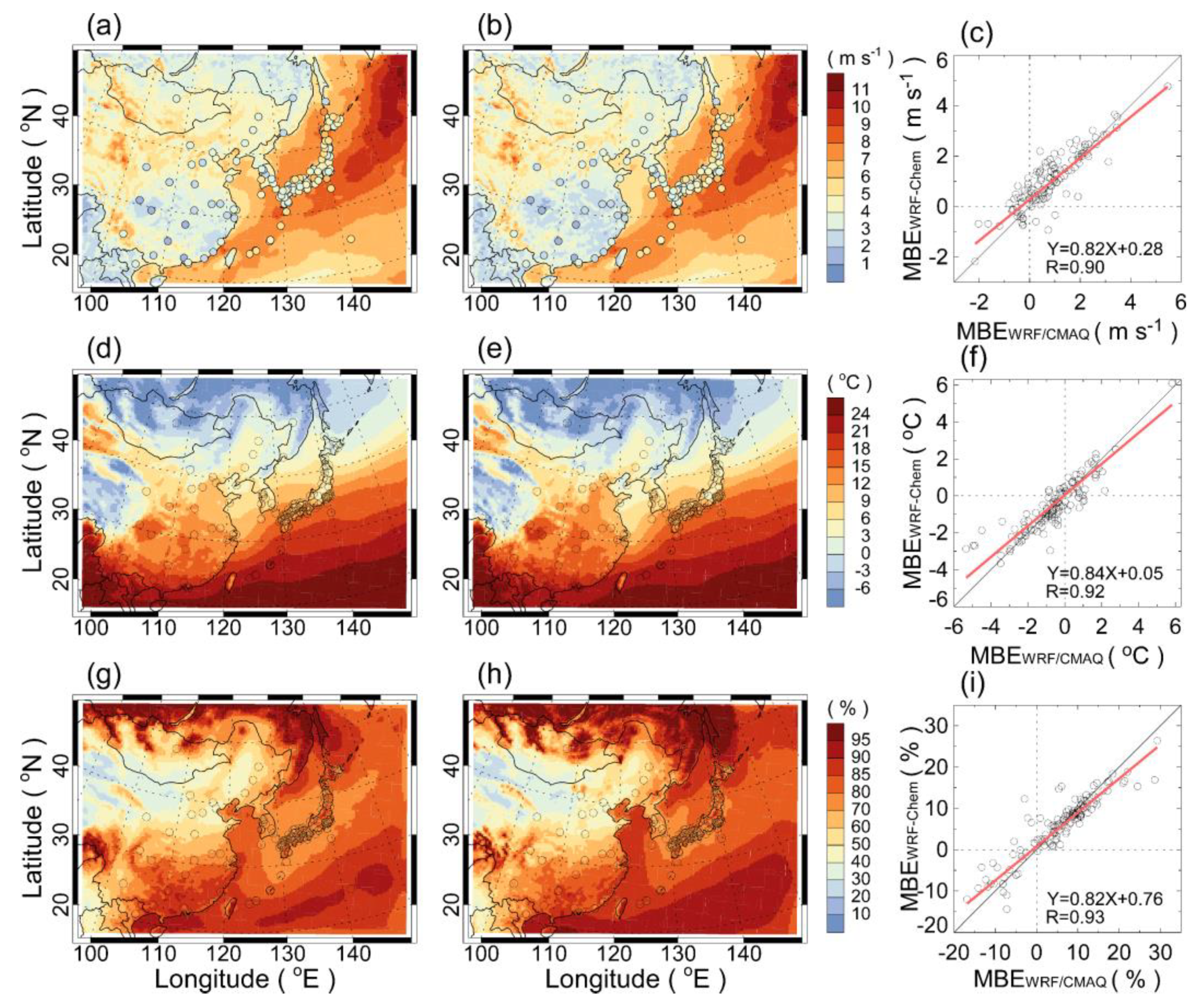
3.1. Evaluation of the Simulated Meteorological Fields

Figure 3 compares the spatial distributions of the simulated 10-m wind speed, 2-m temperature, and relative humidity by the WRF-Chem and WRF/CMAQ models against the measurements, which was used to interpret the surface PM_2.5 chemical components simulated by both the models. The simulated and measured spatial distributions were presented by the 24-days temporal mean values and the MBE values were calculated at the surface measurement sites from hourly simulated and measured data. In the East Asian domain area, the surface wind speeds were relatively higher in most maritime areas than continental areas. The central and southern China regions had relatively weak wind speeds compared to the northern China (Figure 3a,b). The simulated wind speeds in Korea and Japan ranged 2–5 m s⁻¹. The models overestimated the wind speeds at most surface sites with the MBE values ranging from −2 m s⁻¹ up to 5 m s⁻¹ (Figure 3c). The model discrepancy in surface wind speed may be attributed to inaccurate surface drag parameterization (e.g., [32,78]). The surface air temperatures were relatively high in low latitude areas. The Tibetan areas in the central China had relatively low temperatures less than 0 °C due to high altitude (Figure 3d,e). The MBE values of the models similarly ranged from −5 °C to 3 °C, showing frequent underestimation at many surface measurement sites in Korea and Japan (Figure 3d−f). The relative humidity were relatively high in the southern China and most maritime areas due to high moisture availability, which were also high in the northern boundary areas of the simulation domain due to relatively low air temperature (Figure 3g,h). The MBE values of the models ranged from −10% to 30%, showing slight overestimation at most surface measurement sites in Korea and Japan, but slight underestimation at many surface measurement sites in China (Figure 3g–i).

Figure 4 compares the spatial distributions of the monthly mean precipitation and PBL height simulated by the WRF-Chem and WRF/CMAQ models. A prominent precipitation band that is stretching from the southern China, crossing the southern sea of the Korean peninsula to Japan was clearly identified in the TRMM precipitation, which is a characteristic seasonal feature found in the mid-latitude East Asian region [79,80,81]. Meanwhile, most continental areas over the East Asian region had relatively low precipitation amount less than 30 mm mon⁻¹ (Figure 4a). Both the models reasonably captured the characteristic spatial feature found in TRMM. However, the models’ discrepancies were also founded in that the simulated precipitation band was rather narrower than TRMM and the large precipitation simulated near the southern boundary of the simulation domain was not detected in TRMM (Figure 4b,c). Oh et al. [80] had reported similar model discrepancies in their regional climate simulation over the East Asian domain with attributing partly to inaccurate cumulus parameterization. Despite the discrepancies, both the models captured successfully high precipitation in the southern China and Japan and relatively low precipitation in the central and northern China and Korea. The WRF-Chem simulated slightly less precipitation than the WRF/CMAQ model, especially in the precipitation band, which resulted largely from the use of different cumulus parameterizations in the models. Meanwhile, the PBL height was simulated by 800–1000 m in the northern China and 300–800 m in the southern China, Korea, and Japan. The PBL height was relatively high in the continental region where the surface was dry. In addition, it was relatively high over the Kuroshio warm current region where convective marine boundary layer was steadily developed (Figure 4d,e). Overall, the surface meteorological fields simulated by the models compared reasonably well with the measurements and among each other. Though the WRF-Chem model showed slight better agreement with the measurements than the WRF/CMAQ model (Figure 3c,f,i), the models’ performances were very similar with spatial correlations of R = 0.98 in 10-m wind speed, R = 1.00 in 2-m temperature, R = 0.97 in 2-m relative humidity, R = 0.92 in precipitation, and R = 0.97 in PBL height. The meteorological similarities between the two models were expected because the meteorological physics options were assigned identically.

The simulated meteorological differences between the two models were quantified before analyzing meteorological influences on the simulated PM_2.5 chemical components. Figure 5 presents the spatial distributions of relative differences of the simulated meteorological variables between the models along with the mean and FD values at six subdivisions. The red color-coded areas indicate the WRF-Chem model has the higher values than the WRF/CMAQ model and the blue color-coded areas indicate the WRF/CMAQ model has the higher values. The statistical significances of the mean meteorological differences between the two models were tested using a two-sided T-test. The results showed that the WRF-Chem model simulated the higher surface wind speeds, on average, by 0.2 m s⁻¹ ± 0.4 m s⁻¹ over the whole simulation domain than the WRF/CMAQ model. The FD values were less than 10% in the six subdivisions (Figure 5a). The 2-m temperatures by the WRF-Chem model were the lower in the central and southern China than the WRF/CMAQ model, while the differences were opposite in northern parts of the continental region. The differences ranged 0.3 °C ± 0.9 °C with the FD values less than 10% in the six subdivisions (Figure 5b). The differences in relative humidity were negatively correlated with the simulated 2-m temperatures, which ranged −1.8% ± 4.7% with the FD values less than 5% in all the six subdivisions (Figure 5c). As discussed, the WRF-Chem model simulated slightly the lower precipitation in the prominent rain band than the WRF/CMAQ model. The largest differences were found in the southern China and South Korea regions with the FD values of 40–50%. The large FD values were primarily attributed to the use of different cumulus parameterization, which were also found in the regions with low precipitation (Figure 5d). The differences in PBL height ranged 52.1 m ± 84.7 m over the simulation domain with the FD values less than 10% in the subdivisions. The PBL height differences were positively related with the 2-m temperature and negatively related with the relative humidity (Figure 5e). The relatively low 2-m temperature and PBL height and the high relative humidity in WRF-Chem were clearly identified over the central and southern China regions where the PM_2.5 concentrations were relatively high, which resulted primarily from the aerosol-radiation interaction in the online WRF-Chem simulation. The statistical significance test indicated that the models’ meteorological differences were not significant in all the variables for most of the simulation domain within a 95% significance level. This also implies that the meteorological fields predicted by the two models are very similar each other as planned in the experimental design.

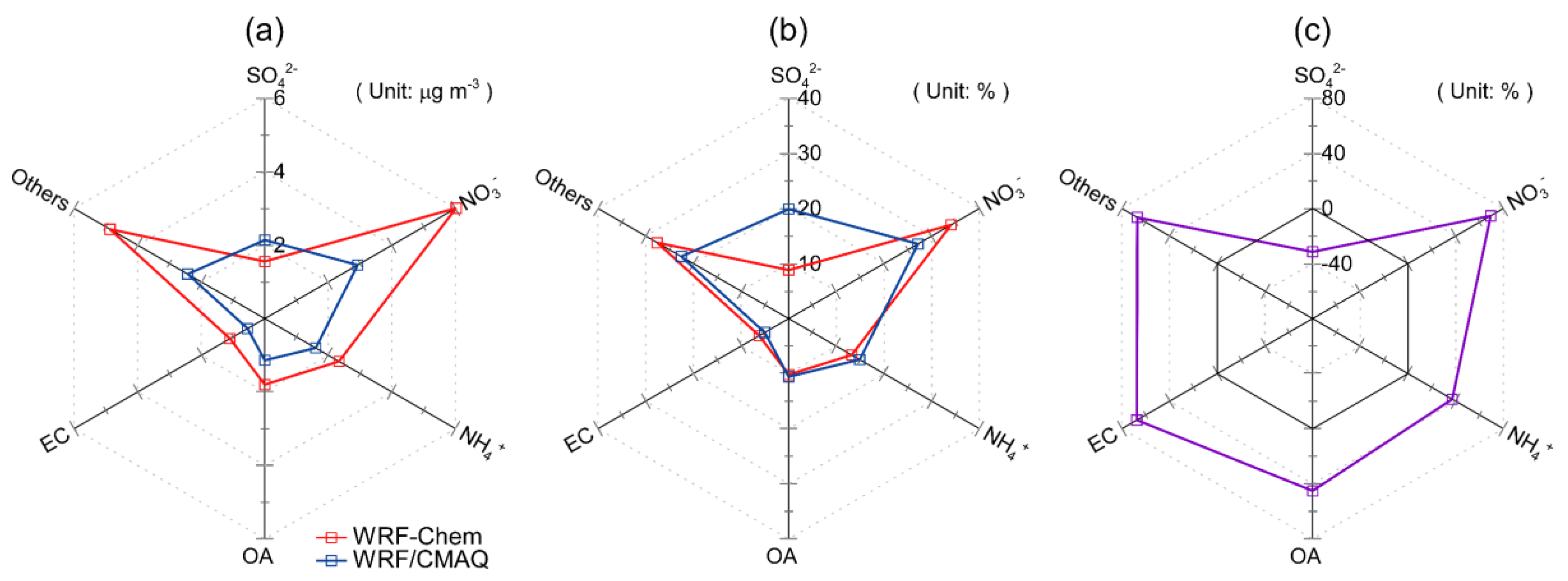
3.2. Characteristics of the Simulated Surface PM_2.5 Chemical Components over East Asia

The surface PM_2.5 chemical components over the East Asian domain simulated by the WRF-Chem and WRF/CMAQ models were compared to identify characteristic features of the PM_2.5 chemical composition and to investigate relative differences between the two models. The PM_2.5 concentration was calculated by the summation of the simulated sulfate (SO₄²⁻), nitrate (NO₃⁻), ammonium (NH₄⁺), organic aerosols (OA), elemental carbon (EC), and other non-reactive PM_2.5 components. The primary natural sources of soil dust and sea salt directly emitted to the atmosphere were calculated at both the models as a function of meteorological and surface conditions. However, those natural contributions to the PM_2.5 concentration were not included in order to investigate the models’ performance and prediction consistency under the emissions controlled identically. Figure 6 presents the spatial distributions of the surface PM_2.5 concentrations simulated by the WRF-Chem and WRF/CMAQ models. At both simulations, the high levels of the PM_2.5 concentration were clearly identified in the central China (R2) where the anthropogenic emissions were high, and followed by the northern and southern China (R1 and R3) and North Korea (R4). The elevated PM_2.5 concentrations in the North and South Korea (R4 and R5) were found more closely associated with the continental polluted areas than Japan (R6) due to the geographical locations (Figure 6a,b). The WRF-Chem model simulated the higher PM_2.5 concentrations than the WRF/CMAQ model for most of the domain, and the concentration differences between the two models were found by 10–50 μg m⁻³ in the central and southern China (Figure 6c). As will be discussed in Figure 7, the large differences at both the regions were contributed by different PM_2.5 chemical components. The temporal variation in the simulated surface PM_2.5 concentration generally increased with the concentration levels at both the models (Figure 6d,e). It was also clearly identified that the WRF-Chem model had the higher temporal and spatial variabilities than the WRF/CMAQ model, which may be attributed largely to online interactions between the meteorological and chemical processes in the WRF-Chem model.

Figure 7 presents the spatial distributions of the surface PM_2.5 chemical components simulated by the WRF-Chem and WRF/CMAQ models to further investigate the models’ inconsistency in simulating the PM_2.5 chemical components. As was explained in the total PM_2.5 concentrations (Figure 6), both the models simulated high concentration levels of the PM_2.5 chemical components in the central China (R2) as a consequence of high anthropogenic emissions. The downwind influences of the continental polluted areas were more clearly identified from the elevated surface concentrations in the North and South Korea (R4 and R5) than Japan (R6), especially in the nitrate (NO₃⁻) and ammonium (NH₄⁺). The long-range influences are because the SIA components formed in the atmosphere during the downwind transport. In contrast, the relatively high concentrations of the organic matters (OA and EC) over the continental polluted areas remained around local emission areas because those chemical components were quickly diluted downwind the continental region. Meanwhile, the relative differences between the WRF-Chem and WRF/CMAQ models were also clearly identified in the atmospheric concentrations as well as the spatial distributions of the simulated PM_2.5 chemical components. In the SIA components, the WRF-Chem model tended to simulate the higher NO₃⁻ and NH₄⁺ concentrations but the lower SO₄²⁻ concentrations than the WRF/CMAQ model. The relative differences varied at different geographical locations showing that the WRF-Chem model simulated relatively high concentrations in the central and southern China but low concentrations in the northern China. The downwind influences of the continental pollution were more clearly identified in the WRF-Chem simulation, especially in NO₃⁻, than the WRF/CMAQ model. For the other three components, the WRF-Chem model simulated the higher concentrations for most source areas than the WRF/CMAQ model. The large model-model concentration differences were found around strong source regions, which were partly attributed to the weaker vertical mixing in the WRF-Chem model (e.g., [28]). Overall, the model-model prediction differences in the simulated surface PM_2.5 chemical components were clear with changing by the geographical locations despite the emissions and meteorological conditions were experimentally controlled.

The analyses were more focused on the model-model differences in the simulated surface PM_2.5 chemical components. Figure 8 compares the surface PM_2.5 chemical components averaged over the East Asian domain simulated by the WRF-Chem and WRF/CMAQ models. The WRF-Chem model simulated the higher concentrations in the PM_2.5 chemical components except for SO₄²⁻ than the WRF/CMAQ model (Figure 8a), while the mass fraction of chemical components at each model was similar to each other (Figure 8b). Tuccella et al. [40] attributed the underestimated sulfate by a factor of 2 to inaccurate representation of aqueous phase oxidation processes of SO₂ by hydrogen peroxide (H₂O₂) and O₃ in the WRF-Chem simulation over Europe. Here, a more prominent result was that the FD values changed significantly ranging from −32% in SO₄²⁻ to 69% in NO₃⁻ (Figure 8c). The results suggest that the large differences between the two models (that is, the models’ prediction inconsistency) can make a significant inconsistency in predicting PM_2.5 forecast and/or supporting policy for a certain region over East Asia if any of the models is applied independently.

To better understand the models’ prediction inconsistency, the surface PM_2.5 chemical components were quantitatively investigated by a fractional difference (FD) over the East Asian domain in Figure 9. The FD value at each grid was calculated as follows:

$$FD(\%)=\frac{\left(C_{WRF-Chem}-C_{\frac{WRF}{CMAQ}}\right)}{0.5\left(C_{WRF-Chem}+C_{\frac{WRF}{CMAQ}}\right)}\times 100,$$

(3)

here, $C$ is the simulated concentration of the PM_2.5 chemical components. The areas where the mean concentration of the two models is less than 1 μg m⁻³ were not included in the analyses. As discussed in Figure 6 and Figure 7, the large chemical differences were found near the source regions and their downwind regions. The model-model differences in PM_2.5 (∆PM_2.5 = C_WRF-Chem-C_WRF/CMAQ) ranged 7.0 μg m⁻³ ± 10.0 μg m⁻³ over the East Asian domain, which corresponded to 53% ± 30% in FD value. The coastal outflow region of the southern China (R3) showed much higher FD values over 120% (max. 141%) than the continental source regions (Figure 9a). For all the six subdivisions, the WRF-Chem model simulated the higher concentrations, on average, than the WRF/CMAQ model (Figure 9b), and the FD values were relatively high by approximately 80% in the southern China (R3) and Japan (R6) (Figure 9c). Unlike the model-model differences in the meteorological variables where no significant inconsistencies were found (Figure 5), the simulated PM_2.5 concentrations showed the large differences between the two models, and the concentration differences were also statistically significant for most regions (green dotted areas in Figure 9a).

Figure 10 shows the spatial distributions of the differences between the two models in each simulated surface PM_2.5 chemical components. The results showed that the models prediction inconsistencies can be characterized by each chemical component. In sulfate, the WRF-Chem model simulated the lower concentrations by −45% ± 33% in FD value (Figure 10a). In nitrate and ammonium components, the WRF-Chem model simulated the higher concentrations, on average, in most subdivisions than the WRF/CMAQ model except in the northern China (R1) (Figure 10b,c). The FD values in nitrate ranged from −59% at R1 to approximately 157% at R6. Meanwhile, the organic aerosols simulated by the WRF-Chem model showed the higher concentrations by 28–70% in FD value for large source regions, except for Japan (R6), than the WRF/CMAQ model (Figure 10d). The underestimation of OA in many AQMs has been frequently reported (e.g., [82,83,84]). The large distinctive differences between the two models were found by up to 50%, on average, in the continental anthropogenic source regions, especially in the central China (Figure 10d). The EC and non-reactive PM_2.5 primary chemical components had very close spatial distributions in the model-model differences ranging 50–80% in FD values at the subdivisions (Figure 10e,f). As both the chemical components were treated as passive tracers in the models, the model-model differences in each component can be attributed to the meteorological influences. Considering that the simulated surface chemical concentrations of OA, EC and Others were very small with less than 1 μg m⁻³ in Japan (R6), both the models had clear systematic inconsistencies in simulating the three chemical components over the domain. Overall, the models’ prediction inconsistencies identified in the simulated PM_2.5 chemical components were statistically significant for most of the regions and very larger than as expected based on the meteorological differences between the two models.

3.3. Meteorological Influences on the Prediction Inconsistencies in the Surface PM_2.5 Chemical Components

The models’ prediction inconsistencies in the surface PM_2.5 chemical components can be caused by the differences from meteorological and chemical processes given the anthropogenic and biogenic emissions were identical. Here, a multiple linear regression (MLR) analyses were applied to better understand the relative influences of the five meteorological variables on the differences in the PM_2.5 concentrations between the two models. The dependent variable is the relative difference of the predicted concentrations (∆C = C_WRF-Chem-C_WRF/CMAQ) and the independent variables (predictors) are the meteorological differences (∆M = M_WRF-Chem-M_WRF/CMAQ) in the 10-m wind speed ($\mathsf{\Delta }WS$), 2-m temperature ($\mathsf{\Delta }T$), relative humidity ($\mathsf{\Delta }RH$), precipitation ($\mathsf{\Delta }Pr$), and PBL height ($\mathsf{\Delta }{h}_{PBL}$). All the dependent and independent variables were normalized before the regression analyses by subtracting each mean value and dividing with standard deviation. The use of normalized variables makes a comparison of relative influences between the independent variables with different units. The MLR relation can be given as:

$$\widehat{\mathsf{\Delta }C}={\displaystyle \sum }_{i=1}^k\left({\beta }_i\mathsf{\Delta }{M}_i\right),$$

(4)

where $\widehat{\mathsf{\Delta }C}$ is the regressed surface PM_2.5 concentration difference between the two models, ${\beta }_i$ is the regression coefficients, and $\mathsf{\Delta }{M}_i$ indicates the difference in the meteorological variable $i$. The regression analysis can give better understanding on the meteorological influences of the large prediction inconsistencies in the simulated PM_2.5 chemical components.

Figure 11 shows the spatial distribution of the determinant coefficients (R²) estimated from the MLR analyses and compares the regression coefficients (${\beta }_i$) of the meteorological factors at six subdivisions. The R² values in the surface PM_2.5 concentration ranged 35% ± 15% at the model grid (Figure 11a), and the determinant coefficients of each chemical component also showed similar mean values of 34–37% and standard deviations of 16–17% (not shown). These results showed that a considerable fraction of the variance in $\mathsf{\Delta }P{M}_{2.5}$ was explained by the meteorological factors despite of the small differences in each $\mathsf{\Delta }{M}_i$. Among the meteorological factors, the regression coefficients showed the largest negative correlation in relative humidity ($\mathsf{\Delta }RH$) followed by precipitation ($\mathsf{\Delta }Pr$), PBL height ($\mathsf{\Delta }{h}_{PBL}$), 10-m wind speed ($\mathsf{\Delta }WS$), and 2-m temperature ($\mathsf{\Delta }T$) for the whole domain. In contrast, the precipitation difference ($\mathsf{\Delta }Pr$) showed a relatively high positive correlation. The relative importance of the meteorological differences changed with geographical locations at six subdivisions (Figure 6b). For example, $\mathsf{\Delta }RH$ had the largest negative correlation in R1-R3, which was not in the other downwind regions. When considered at each region, the variance in $\mathsf{\Delta }P{M}_{2.5}$ was explained by $\mathsf{\Delta }{M}_i$ was approximately 40% in the northern and central China (R1 and R2), about 55% in the southern China (R3), and the maximum correlation was found over 80% in South Korea (R5). The Japanese region (R6) showed a relatively low correlation of approximately 20%.

In order to explain the high sensitivity of the meteorological factors on $\mathsf{\Delta }P{M}_{2.5}$, each term in the above MLR equation can be split into two parts with a simple assumption. The MLR relation between $P{M}_{2.5}$ and $M_i$ for each model can be expressed by:

$$\widehat{C}={\alpha }_0+{{\displaystyle \sum }}_{i=1}^k\left({\beta }_i{M}_i\right),$$

(5)

where $\widehat{C}$ is the regressed PM_2.5 concentration, ${\alpha }_0$ is the regression constant. From the difference of the multiple regression relations of the two model $\mathsf{\Delta }\widehat{C} \left(={\widehat{C}}_{WRF-Chem}-{\widehat{C}}_{WRF/CMAQ}\right)$, the $\widehat{\mathsf{\Delta }C}$ can be approximated as

$$\widehat{\mathsf{\Delta }C}\cong \mathsf{\Delta }{\alpha }_0+{{\displaystyle \sum }}_{i=1}^k\left(M_i^{WRF-Chem}\mathsf{\Delta }{\beta }_i+{\beta }_i^{WRF/CMAQ}\mathsf{\Delta }{M}_i\right),$$

(6)

where $\mathsf{\Delta }{\beta }_{\mathrm{i}}\left(={\beta }_i^{WRF-Chem}-{\beta }_i^{WRF/CMAQ}\right)$ and $\mathsf{\Delta }{M}_i\left(=M_i^{WRF-Chem}-M_i^{WRF/CMAQ}\right)$ are the differences in ${\beta }_{\mathrm{i}}$ and $M_i$ between the WRF-Chem and WRF/CMAQ models, respectively. The regression coefficient ${\beta }_{\mathrm{i}}\left(=\frac{\partial C}{\partial M_i}\right)$ can be interpreted as a prediction response of surface PM_2.5 concentration to each meteorological factor. From the separated regression relation, the first and second terms in parenthesis explain the contributions of $\mathsf{\Delta }P{M}_{2.5}$ by $\mathsf{\Delta }{\beta }_{\mathrm{i}}$ (‘difference on chemical responses by meteorology’; term A) and $\mathsf{\Delta }{M}_i$ (‘meteorological difference’; term B). The MLR results showed that the correlation coefficients between the surface PM_2.5 concentrations and the meteorological factors in each model ranged 53% ± 19% in WRF-Chem and 48% ± 15% in WRF/CMAQ. The higher R² values in WRF-Chem imply that the online model has the stronger coupling between the meteorological and chemical processes than WRF/CMAQ. Figure 12 compares the relative contribution of the difference on chemical response by meteorology (term A) and the meteorological difference (term B) within the MLR equation. The precipitation difference between the two models had relatively large contribution in term B by approximately 30%, but the term A were predominant compared to the term B in all the other meteorological variables. This result explained why the surface PM_2.5 chemical components were significantly different between the two models despite the differences in the simulated meteorological variables were negligible. In other words, the result showed that the model-model differences in ${\beta }_{\mathrm{i}}$ were large enough to make the significant differences in the surface PM_2.5 chemical components between the two models.

Figure 13 compares the ${\beta }_{\mathrm{i}}$ values of the WRF-Chem and WRF/CMAQ models estimated from the linear regression analyses at each grid of the domain. The PM_2.5 concentrations in both the two models were correlated with the meteorological variables negatively (3rd quadrant) at most regions, and positively (1st quadrant) at some regions. The two models had the ${\beta }_{\mathrm{i}}$ values with different signs (2nd and 4th quadrants) at approximately 10–20% regions, which indicates the model’s prediction response of surface PM_2.5 concentration to the meteorological factor is opposite each other. Overall, the WRF-Chem model had the larger values than the WRF/CMAQ model, indicating that the former is more sensitive to the meteorological variables than the latter. The analysis result confirmed that the large model-model differences in ${\beta }_{\mathrm{i}}$ can explain the significant differences in the surface PM_2.5 chemical components between the WRF-Chem and WRF/CMAQ models.

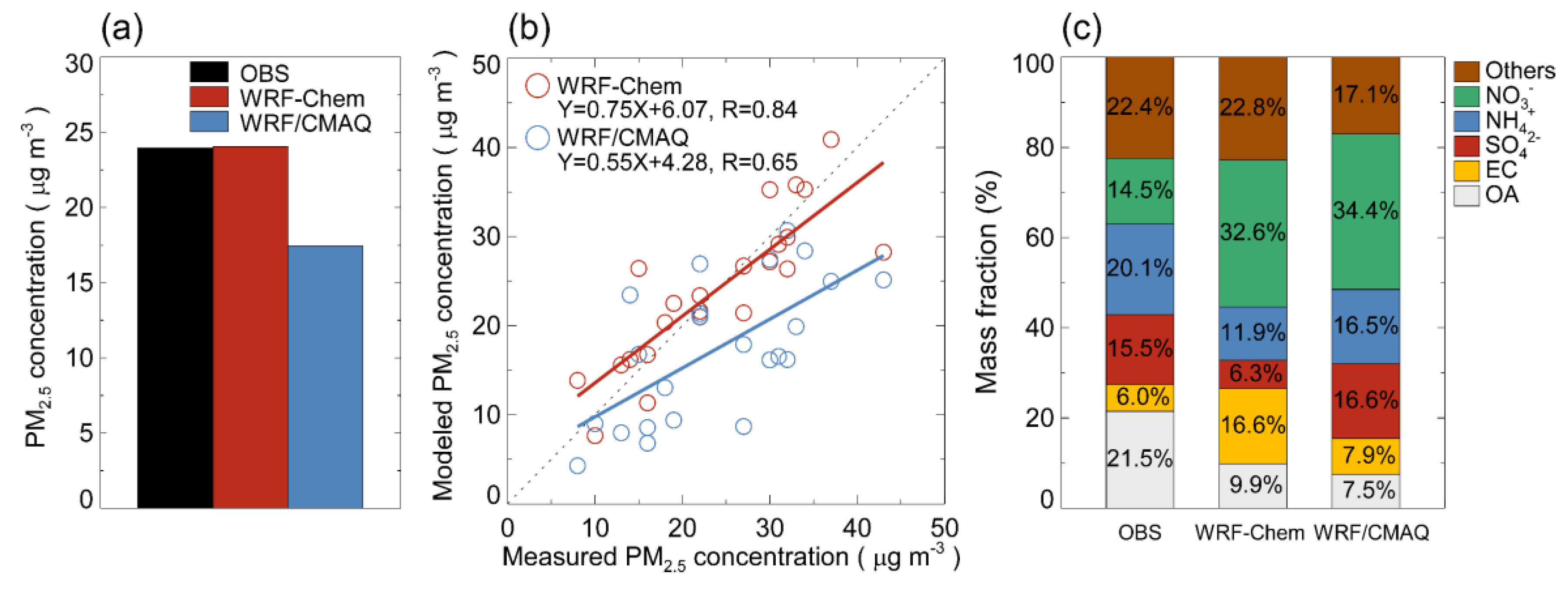
3.4. Evaluation of the Simulated PM_2.5 Chemical Components in South Korea

Finally, the simulated PM_2.5 chemical components were compared against measurements at Seoul, South Korea (R5) in Figure 14 to evaluate the models’ performances shortly. The natural soil dust and sea salt aerosols simulated by the models were included in the total PM_2.5 concentrations for comparison with the measurements. The comparison showed that the WRF-Chem model simulated the 24-days mean surface PM_2.5 concentrations better than the WRF-Chem model (Figure 14a). The performance in predicting the daily mean PM_2.5 concentrations was also superior in the WRF-Chem model (R = 0.84) compared to the WRF/CMAQ model (R = 0.65) (Figure 14b). The mean fractional bias (MFB) values were 0.02 in WRF-Chem and −0.34 in WRF/CMAQ. Ghim et al. [85] reported a similar model forecast performance of R = 0.68 and MFB = −0.36 for Seoul during the period May 2012 to December 2014 using a WRF/CMAQ forecast system. Though the WRF-Chem model performed better in simulating the total surface PM_2.5 concentration than the WRF/CMAQ model, the mass fraction of the chemical compositions was compared differently between the two models (Figure 14c).

Table 2. The measured and simulated monthly mean PM_2.5 chemical components over Seoul, South Korea in April 2010. The numbers in parentheses denote the fractional biases.

	OBS	WRF-Chem	WRF/CMAQ
Sulfate	3.6	1.4 (−0.88)	2.9 (−0.22)
Nitrate	3.4	7.2 (0.72)	6.0 (0.55)
Ammonium	4.7	2.6 (−0.58)	2.9 (−0.47)
Elemental carbon (EC)	1.4	3.7 (0.90)	1.4 (0.0)
Organic aerosols (OA)	5.0 1	2.2 (−0.78)	1.3 (−1.18)
Others	5.2	5.1 (−0.02)	3.0 (−0.54)
Total PM2.5	23.3	22.2 (−0.05)	17.5 (−0.28)

¹ The ratio of organic matters to organic carbon is applied with 1.6.

compares the measured and simulated monthly mean PM_2.5 chemical components in Seoul April 2010. The measured sulfate and ammonium aerosols were underestimated by both the models, while the nitrate aerosols were overestimated. The OA was underestimated by −78% in WRF-Chem and −118% in WRF/CMAQ. The EC was well simulated by the WRF/CMAQ model, but overestimated by the WRF-Chem model, meanwhile the non-reactive PM_2.5 chemical component was better simulated by the WRF-Chem model than the WRF/CMAQ model. These results indicated that the WRF-Chem can give a better performance than the WRF/CMAQ model in predicting the surface PM_2.5 concentrations but the model’s discrepancies in chemical composition should be further improved.

The models’ prediction inconsistencies were also identified with the FD values of 23.7% in PM_2.5, −69.8% in sulfate, 18.2% in nitrate, −10.9% in ammonium, 51.4% in OA, 90.2% in EC, and 62.1% in non-reactive PM_2.5 chemical component.

4. Summary and Conclusions

Two high-fidelity air quality models of the WRF-Chem and WRF/CMAQ models has been compared to investigate the models’ prediction inconsistencies in simulating the surface PM_2.5 chemical components over the East Asian region. The models have been frequently used for the PM_2.5 forecasts and policy support over the East Asian countries to cope with environmental issues associated with high levels of the atmospheric PM_2.5 concentrations. However, an attention of the models’ prediction consistency, which is prerequisite for accurate forecasts and reliable policy support, has not been paid. For the purpose, the PM_2.5 chemical components over the East Asian domain was simulated by the WRF-Chem and WRF/CMAQ models with a uniquely designed experimental setup in meteorological, chemical, and emissions processes. From the simulation results, the significant model-model prediction inconsistencies in the surface PM_2.5 chemical components were identified throughout the East Asian domain despite the simulated meteorological differences were minimal with FB values less than approximately 10% and the anthropogenic and biogenic emissions were identical. The WRF-Chem model simulated the higher surface PM_2.5 concentration by 53% ± 30% than the WRF/CMAQ model for most continental source regions in China and downwind regions in Korea and Japan. The prediction inconsistencies were the most prominent for nitrate aerosols in the PM_2.5 chemical components, ranging from −59% at R1 to approximately 157% at R6. The MLR analyses revealed that the models’ prediction inconsistencies between the two models were largely attributed to the sensitivity of chemical responses to meteorology, which were significantly different between the models in five meteorological variables, rather than the influence by the meteorological differences. Finally, the comparison of the simulated surface PM_2.5 chemical components against surface measurements at a site in South Korea showed the WRF-Chem model (MBE = 0.02) performed better in daily mean PM_2.5 prediction than the WRF/CMAQ model (MBE = −0.34) and both the models’ discrepancies were also identified in the PM_2.5 chemical composition as well as in total concentration.

Many studies used one of the air quality models for local PM_2.5 forecasts (e.g., [27,35]), top-down emissions verification (e.g., [36,37]), and environmental policy decision (e.g., [24]). The results of this study imply that the models’ prediction inconsistencies should be considered in these applications so as not to be biased in interpreting the model results due to the significant prediction inconsistencies in simulating the surface PM_2.5 chemical components, especially in the continental source region and downwind region over the East Asian domain.

In this study, the ‘online’ WRF-Chem model showed a tighter coupling between the simulated meteorology and the PM_2.5 chemical components than the ‘offline’ WRF/CMAQ model, which was identified from the higher correlation between the simulated meteorological variables and PM_2.5 chemical components as well as surface measurements. In this sense, the WRF-Chem model has an intrinsic potential in simulating surface PM_2.5 chemical components in a more realistic manner. However, more research is needed to improve the parameterizations of natural sources (e.g., soil dust, sea salt) and to evaluate turbulent mixing processes in the PBL against faithful measurements.

References

1. International Agency for Research on Cancer; World Health Organization (WHO). IARC: Outdoor Air Pollution a Leading Environmental Cause of Cancer Deaths; WHO: Geneva, Switzerland, 2013. [Google Scholar]
2. Ostro, B.; Broadwin, R.; Green, S.; Feng, W.-Y.; Lipsett, M. Fine particulate air pollution and mortality in nine California counties: Results from CALFINE. Environ. Health Perspect. 2006, 114, 29–33. [Google Scholar] [CrossRef] [PubMed]
3. Ostro, B.; Feng, W.-Y.; Broadwin, R.; Green, S.; Lipsett, M. The effects of components of fine particulate air pollution on mortality in California: Results from CALFINE. Environ. Health Perspect. 2007, 115, 13–19. [Google Scholar] [CrossRef] [PubMed]
4. Son, J.Y.; Lee, J.T.; Kim, K.H.; Jung, K.; Bell, M.L. Characterization of fine particulate matter and associations between particulate chemical constituents and mortality in Seoul, Korea. Environ. Health Perspect. 2012, 120, 872. [Google Scholar] [CrossRef] [PubMed]
5. Han, L.; Zhou, W.; Li, W.; Li, L. Impact of urbanization level on urban air quality: A case of fine particles PM2.5 in Chinese cities. Environ. Pollut. 2014, 194, 163–170. [Google Scholar] [CrossRef]
6. Pascal, M.; Falq, G.; Wagner, V.; Chatignoux, E.; Corso, M.; Blanchard, M.; Host, S.; Pascal, L.; Larrieu, S. Short-term impacts of particulate matter (PM10, PM10–2.5, PM2.5) on mortality in nine French cities. Atmos. Environ. 2014, 95, 175–184. [Google Scholar] [CrossRef]
7. Song, C.; Pei, T.; Yao, L. Analysis of the characteristics and evolution modes of PM2.5 pollution episodes in Beijing, China during 2013. Int. J. Environ. Res. Public Health 2015, 12, 1099–1111. [Google Scholar] [CrossRef]
8. Liang, C.S.; Duan, F.K.; He, K.B.; Ma, Y.L. Review on recent progress in observations, source identifications and countermeasures of PM2. 5. Environ. Int. 2016, 86, 150–170. [Google Scholar] [CrossRef]
9. Laden, F.; Neas, L.M.; Dockery, D.W.; Schwartz, J. Association of fine particulate matter from different sources with daily mortality in six U.S. cities. Environ. Health Perspect. 2000, 108, 941–947. [Google Scholar] [CrossRef]
10. Takemura, T.; Kaufman, Y.J.; Remer, L.A.; Nakajima, T. Two competing pathways of aerosol effects on cloud and precipitation formation. Geophys. Res. Lett. 2007, 34, L04802. [Google Scholar] [CrossRef]
11. Bey, I.; Jacob, D.J.; Yantosca, R.M.; Logan, J.A.; Field, B.D.; Fiore, A.R.; Li, Q.; Liu, H.Y.; Mickley, L.J.; Schultz, M.G. Quantifying pollution inflow and outflow over East Asia in spring with regional and global models. J. Geophys. Res. 2001, 106, 23073–23095. [Google Scholar] [CrossRef]
12. Park, R.S.; Han, K.M.; Song, C.H.; Park, M.E.; Lee, S.J.; Hong, S.Y.; Kim, J.; Woo, J.H. Current status and development of modeling techniques for forecasting and monitoring of air quality over East Asia. J. KOSAE 2013, 29, 407–438. [Google Scholar] [CrossRef]
13. Park, R.J.; Kim, S.W. Air quality modeling in East Asia: Present issues and future directions. Asia Pac. J. Atmos. Sci. 2014, 50, 105–120. [Google Scholar] [CrossRef]
14. Binkowski, F.S.; Roselle, S.J. Models−3 community multiscale air quality (CMAQ) model aerosol component 1. Model description. J. Geophys. Res. 2003, 108, 4183. [Google Scholar] [CrossRef]
15. Byun, D.; Schere, K.L. Review of the governing equations, computational algorithms, and other components of the models−3 community multiscale air quality (CMAQ) modeling system. Appl. Mech. Rev. 2006, 59, 51–77. [Google Scholar] [CrossRef]
16. Grell, G.A.; Peckham, S.E.; Schmitz, R.; McKeen, S.A.; Frost, G.; Skamarock, W.C.; Eder, B. Fully coupled “online” chemistry within the WRF model. Atmos. Environ. 2005, 39, 6957–6975. [Google Scholar] [CrossRef]
17. Liu, L.-J.S.; Curjuric, I.; Keidel, D.; Heldstab, J.; Künzli, N.; Bayer-Oglesby, L.; Ackermann-Liebrich, U.; Schindler, C.; Team the SAPALDIA. Characterization of source-specific air pollution exposure for a large population-based Swiss cohort (SAPALDIA). Environ. Health Perspect. 2007, 115, 1638–1645. [Google Scholar] [CrossRef]
18. Cohen, M.A.; Adar, S.D.; Allen, R.W.; Avol, E.; Curl, C.L.; Gould, T.; Hardie, A.; Ho, A.; Kinney, P.; Larson, T.V.; et al. Approach to estimating participant pollutant exposures in the multi-ethnic study of atherosclerosis and air pollution (MESA Air). Environ. Sci. Technol. 2009, 43, 4687–4693. [Google Scholar] [CrossRef]
19. Ritter, M.; Müller, M.D.; Jorba, O.; Parlow, E.; Sally Liu, L.-J. Impact of chemical and meteorological boundary and initial conditions on air quality modeling: WRF-Chem sensitivity evaluation for a European domain. Meteorol. Atmos. Phys. 2013, 119, 59–70. [Google Scholar] [CrossRef]
20. El-Harbawi, M. Air quality modelling, simulation, and computational methods: A review. Environ. Rev. 2013, 21, 149–179. [Google Scholar] [CrossRef]
21. Fuzzi, S.; Baltensperger, U.; Carslaw, K.; Decesari, S.; Denier van der Gon, H.; Facchini, M.C.; Fowler, D.; Koren, I.; Langford, B.; Lohmann, U.; et al. Particulate matter, air quality and climate: Lessons learned and future needs. Atmos. Chem. Phys. 2015, 15, 8217–8299. [Google Scholar] [CrossRef]
22. Appel, K.W.; Chemel, C.; Roselle, S.J.; Francis, X.V.; Hu, R.-M.; Sokhi, R.S.; Rao, S.T.; Galmarini, S. Examination of the community multiscale air quality (CMAQ) model performance over the North American and European domains. Atmos. Environ. 2012, 53, 142–155. [Google Scholar] [CrossRef]
23. Zhang, H.; Chen, G.; Hu, J.; Chen, S.-H.; Wiedinmyer, C.; Kleeman, M.; Ying, Q. Evaluation of a seven-year air quality simulation using the weather research and forecasting (WRF)/community multiscale air quality (CMAQ) models in the eastern United States. Sci. Total Environ. 2014, 473, 275–285. [Google Scholar] [CrossRef] [PubMed]
24. Lang, J.; Cheng, S.; Li, J.; Chen, D.; Zhou, Y.; Wei, X.; Han, L.; Wang, H. A monitoring and modeling study to investigate regional transport and characteristics of PM2.5 pollution. Aerosol Air Qual. Res. 2013, 13, 943–956. [Google Scholar] [CrossRef]
25. Qin, M.; Wang, X.; Hu, Y.; Huang, X.; He, L.; Zhong, L.; Song, Y.; Hu, M.; Zhang, Y. Formation of particulate sulfate and nitrate over the pearl river delta in the fall: Diagnostic analysis using the community multiscale air quality model. Atmos. Environ. 2015, 112, 81–89. [Google Scholar] [CrossRef]
26. Song, C.H.; Park, M.E.; Lee, K.H.; Ahn, H.J.; Lee, Y.; Kim, J.Y.; Han, K.M.; Kim, J.; Ghim, Y.S.; Kim, Y.J. An investigation into seasonal and regional aerosol characteristics in East Asia using model-predicted and remotely-sensed aerosol properties. Atmos. Chem. Phys. 2008, 8, 6627–6654. [Google Scholar] [CrossRef] [Green Version]
27. Zhou, G.; Xu, J.; Xie, Y.; Chang, L.; Gao, W.; Gu, Y.; Zhou, J. Numerical air quality forecasting over eastern China: An operational application of WRF-Chem. Atmos. Environ. 2017, 153, 94–108. [Google Scholar] [CrossRef]
28. Matsui, H.; Koike, M.; Kondo, Y.; Takegawa, N.; Kita, K.; Miyazaki, Y.; Hu, M.; Chang, S.-Y.; Blake, D.R.; Fast, J.D.; et al. Spatial and temporal variations of aerosols around Beijing in summer 2006: Model evaluation and source apportionment. J. Geophys. Res. 2009, 114, D00G13. [Google Scholar] [CrossRef]
29. Wilczak, J.M.; Djalalova, I.; McKeen, S.; Bianco, L.; Bao, J.-W.; Grell, G.; Peckham, S.; Mathur, R.; McQueen, J.; Lee, P. Analysis of regional meteorology and surface ozone during the TexAQS II field program and an evaluation of the NMM-CMAQ and WRF-Chem air quality models. J. Geophys. Res. 2009, 114, D00F14. [Google Scholar] [CrossRef]
30. Lin, M.; Holloway, T.; Carmichael, G.R.; Fiore, A.M. Global modeling of tropospheric chemistry with assimilated meteorology: Model description and evaluation. Atmos. Chem. Phys. 2010, 10, 4221–4239. [Google Scholar] [CrossRef]
31. Herwehe, J.A.; Otte, T.L.; Mathur, R.; Rao, S.T. Diagnostic analysis of ozone concentrations simulated by two regional-scale air quality models. Atmos. Environ. 2011, 45, 5957–5969. [Google Scholar] [CrossRef]
32. Zhang, Y.; Zhang, X.; Wang, L.; Zhang, Q.; Duan, F.; He, K. Application of WRF/Chem over East Asia: Part I. Model evaluation and intercomparison with MM5/CMAQ. Atmos. Environ. 2016, 124, 285–300. [Google Scholar] [CrossRef]
33. Zhang, Y.; Zhang, X.; Wang, K.; Zhang, Q.; Duan, F.; He, K. Application of WRF/Chem over East Asia: Part Ⅱ. Model improvement and sensitivity simulations. Atmos. Environ. 2016, 124, 301–320. [Google Scholar] [CrossRef]
34. Skamarock, W.C.; Klemp, J.B. A time-split nonhydrostatic atmospheric model for weather research and forecasting applications. J. Comput. Phys. 2008, 227, 3465–3485. [Google Scholar] [CrossRef]
35. Wang, T.; Jiang, F.; Deng, J.; Shen, Y.; Fu, Q.; Wang, Q.; Fu, Y.; Xu, J.; Zhang, D. Urban air quality and regional haze weather forecast for Yangtze River Delta region. Atmos. Environ. 2012, 58, 70–83. [Google Scholar] [CrossRef]
36. Goldberg, D.L.; Saide, P.E.; Lamsal, L.N.; de Foy, B.; Lu, Z.; Woo, J.-H.; Kim, Y.; Kim, J.; Gao, M.; Carmichael, G. A top-down assessment using OMI NO2 suggests an underestimate in the NOX emissions inventory in Seoul, South Korea, during KOURS-AQ. Atmos. Chem. Phys. 2019, 19, 1801–1818. [Google Scholar] [CrossRef]
37. Lee, J.-H.; Lee, S.-H.; Kim, H.C. Detection of strong NOX emissions from fine-scale reconstruction of the OMI tropospheric NO2 product. Remote Sens. 2019, 11, 1861. [Google Scholar] [CrossRef]
38. Kim, S.-W.; Heckel, A.; Frost, G.J.; Richter, A.; Gleason, J.; Burrows, J.P.; McKeen, S.; Hsie, E.-Y.; Granier, C.; Trainer, M. NO2 columns in the western United States observed from space and simulated by a regional chemistry model and their implications for NOX emissions. J. Geophys. Res. 2009, 114, D11301. [Google Scholar] [CrossRef]
39. Lee, S.-H.; Kim, S.-W.; Trainer, M.; Frost, G.J.; McKeen, S.A.; Cooper, O.R.; Flocke, F.; Holloway, J.S.; Neuman, J.A.; Ryerson, T.; et al. Modeling ozone plumes observed downwind of New York City over the North Atlantic Ocean during the ICARTT field campaign. Atmos. Chem. Phys. 2011, 11, 7375–7397. [Google Scholar] [CrossRef] [Green Version]
40. Tuccella, P.; Curci, G.; Visconti, G.; Bessagnet, B.; Menut, L.; Park, R.J. Modeling of gas and aerosol with WRF/Chem over Europe: Evaluation and sensitivity study. J. Geophys. Res. 2012, 117, D3303. [Google Scholar] [CrossRef]
41. Han, K.M.; Song, C.H. A budget analysis of NOx column losses over the Korean peninsula. Asia Pac. J. Atmos. Sci. 2012, 48, 55–65. [Google Scholar] [CrossRef]
42. Lee, J.-H.; Chang, L.-S.; Lee, S.-H. Simulation of air quality over South Korea using the WRF-Chem model: Impacts of chemical initial and lateral boundary conditions. Atmosphere 2015, 25, 639–657. [Google Scholar] [CrossRef]
43. Tong, D.Q.; Lamsal, L.; Pan, L.; Ding, C.; Kim, H.; Lee, P.; Chai, T.; Pickering, K.E.; Stajner, I. Long-term NOX trends over large cities in the United States during the great recession: Comparison of satellite retrievals, ground observations, and emission inventories. Atmos. Environ. 2015, 107, 70–84. [Google Scholar] [CrossRef]
44. Otte, T.L.; Pleim, J.E. The meteorology-chemistry interface processor (MCIP) for the CMAQ modeling system: Updates through MCIPv3.4.1. Geosci. Model Dev. 2010, 3, 243–256. [Google Scholar] [CrossRef]
45. Dudhia, J. Numerical study of convection observed during the winter monsoon experiment using a mesoscale two-dimensional model. J. Atmos. Sci. 1989, 46, 3077–3107. [Google Scholar] [CrossRef]
46. Iacono, M.J.; Delamere, J.S.; Mlawer, E.J.; Shephard, M.W.; Clough, S.A.; Collins, W.D. Radiative forcing by long-lived greenhouse gases: Calculations with the AER radiative transfer models. J. Geophys. Res. 2008, 113, D13103. [Google Scholar] [CrossRef]
47. Hong, S.-Y.; Noh, Y.; Dudhia, J. A new vertical diffusion package with an explicit treatment of entrainment processes. Mon. Weather Rev. 2006, 134, 2318–2341. [Google Scholar] [CrossRef]
48. Chen, F.; Dudhia, J. Coupling an advanced land surface-hydrology model with the Penn State-NCAR MM5 modeling system. Part I: Model implementation and sensitivity. Mon. Weather Rev. 2001, 129, 569–585. [Google Scholar] [CrossRef]
49. Hong, S.-Y.; Dudhia, J.; Chen, S.H. A revised approach to ice microphysical processes for the bulk parameterization of clouds and precipitation. Mon. Weather Rev. 2004, 132, 103–120. [Google Scholar] [CrossRef]
50. Grell, G.A.; Freitas, S.R. A scale and aerosol aware stochastic convective parameterization for weather and air quality modeling. Atmos. Chem. Phys. 2013, 13, 23845–23893. [Google Scholar] [CrossRef]
51. Kain, J.S. The Kain–Fritsch convective parameterization: An update. J. Appl. Meteor. 2004, 43, 170–181. [Google Scholar] [CrossRef]
52. Stockwell, W.R.; Kirchner, F.; Kuhn, M.; Seefeld, S. A new mechanism for regional atmospheric chemistry modeling. J. Geophys. Res. 1997, 102, 25847–25879. [Google Scholar] [CrossRef] [Green Version]
53. Ackermann, I.J.; Hass, H.; Memmesheimer, M.; Ebel, A.; Binkowski, F.S.; Shankar, U. Modal aerosol dynamics model for Europe: Development and first applications. Atmos. Environ. 1998, 32, 2981–2999. [Google Scholar] [CrossRef]
54. Schell, B.; Ackermann, I.J.; Hass, H.; Binkowski, F.S.; Ebel, A. Modeling the formation of secondary organic aerosol within a comprehensive air quality model system. J. Geophys. Res. 2001, 106, 28275–28293. [Google Scholar] [CrossRef]
55. Cater, W.P.L. Documentation of the SAPRC−99 Chemical Mechanism for VOC Reactivity Assessment. Final Report to the California Air Resources Board 2000. Available online: https://intra.engr.ucr.edu/~carter/pubs/s99doc.pdf (accessed on 5 September 2019).
56. Foley, K.M.; Roselle, S.J.; Appel, K.W.; Bhave, P.V.; Pleim, J.E.; Otte, T.L.; Mathur, R.; Sarwar, G.; Young, J.O.; Gilliam, R.C.; et al. Incremental testing of the community multiscale air quality (CMAQ) modeling system version 4.7. Geosci. Model Dev. 2010, 3, 205–226. [Google Scholar] [CrossRef]
57. Hutzell, W.T.; Luecken, D.J.; Appel, K.W.; Carter, W.P.L. Interpreting predictions from the SAPRC07 mechanism based on regional and continental simulations. Atmos. Environ. 2012, 46, 417–429. [Google Scholar] [CrossRef]
58. Stauffer, D.R.; Seaman, N.L. Use of four-dimensional data assimilation in a limited-area mesoscale model: Part I: Experiments with synoptic-scale data. Mon. Weather Rev. 1990, 118, 1250–1277. [Google Scholar] [CrossRef]
59. Carmichael, G.R.; Calori, G.; Hayami, H.; Uno, I.; Cho, S.-Y.; Engardt, M.; Kim, S.-B.; Ichikawa, Y.; Ikeda, Y.; Woo, J.-H.; et al. The MICS-Asia study: Model intercomparison of long-range transport and sulfur deposition in East Asia. Atmos. Environ. 2002, 36, 175–199. [Google Scholar] [CrossRef]
60. Li, M.; Zhang, Q.; Kurokawa, J.-I.; Woo, J.-H.; He, K.; Lu, Z.; Ohara, T.; Song, Y.; Streets, D.G.; Carmichael, G.R.; et al. MIX: A mosaic Asian anthropogenic emission inventory under the international collaboration framework of the MICS-Asia and HTAP. Atmos. Chem. Phys. 2017, 17, 935–963. [Google Scholar] [CrossRef]
61. Kurokawa, J.; Ohara, T.; Morikawa, T.; Hanayama, S.; Janssens-Maenhout, G.; Fukui, T.; Kawashima, K.; Akimoto, H. Emissions of air pollutants and greenhouse gases over Asian regions during 2000–2008: Regional Emission inventory in Asia (REAS) version 2. Atmos. Chem. Phys. 2013, 13, 11019–11058. [Google Scholar] [CrossRef]
62. Lee, D.G.; Lee, Y.-M.; Jang, K.-W.; Yoo, C.; Kang, K.-H.; Lee, J.-H.; Jung, S.-W.; Park, J.-M.; Lee, S.-B.; Han, J.-S.; et al. Korean national emissions inventory system and 2007 air pollutant emissions. Asian J. Atmos. Environ. 2011, 5, 278–291. [Google Scholar] [CrossRef]
63. Benjey, W.; Houyoux, M.; Susick, J. Implementation of the SMOKE Emission Data Processor and SMOKE Tool Input Data Processor in Models−3. U.S. EPA; 2001. Available online: https://nepis.epa.gov/Exe/ZyPDF.cgi/P100P6M5.PDF?Dockey=P100P6M5.PDF (accessed on 9 September 2019).
64. Pfister, G.G.; Wiedinmyer, C.; Emmons, L.K. Impacts of fall 2007 California wildfires on surface ozone: Integrating local observations with global model simulations. Geophys. Res. Lett. 2008, 35, L19814. [Google Scholar] [CrossRef]
65. Van Donkelaar, A.; Martin, R.V.; Park, R.J.; Heald, C.L.; Fu, T.-M.; Liao, H.; Guenther, A. Model evidence for a significant source of secondary organic aerosol from isoprene. Atmos. Environ. 2007, 41, 1267–1274. [Google Scholar] [CrossRef]
66. Hallquist, M.; Wenger, J.C.; Baltensperger, U.; Rudich, Y.; Simpson, D.; Claeys, M.; Dommen, J.; Donahue, N.M.; George, C.; Goldstein, A.H.; et al. The formation, properties and impact of secondary organic aerosol: Current and emerging issues. Atmos. Chem. Phys. 2009, 9, 5155–5236. [Google Scholar] [CrossRef]
67. Guenther, A.; Hewitt, C.N.; Erickson, D.; Fall, R.; Geron, C.; Graedel, T.; Harley, P.; Klinger, L.; Lerdau, M.; Mckay, W.A.; et al. Global-model of natural volatile organic-compound emissions. J. Geophys. Res. 1995, 100, 8873–8892. [Google Scholar] [CrossRef]
68. Rosenstiel, T.N.; Potosnak, M.J.; Griffin, K.L.; Fall, R.; Monson, R.K. Increased CO2 uncouples growth from isoprene emission in an agriforest ecosystem. Nature 2003, 421, 256–259. [Google Scholar] [CrossRef]
69. Velikova, V.; Pinelli, P.; Pasqualini, S.; Reale, L.; Ferranti, F.; Loreto, F. Isoprene decreases the concentration of nitric oxide in leaves exposed to elevated ozone. New Phytol. 2005, 166, 419–426. [Google Scholar] [CrossRef]
70. Guenther, A.; Karl, T.; Harley, P.; Wiedinmyer, C.; Palmer, P.I.; Geron, C. Estimates of global terrestrial isoprene emissions using MEGAN (Model of Emissions of Gases and Aerosols from Nature). Atmos. Chem. Phys. 2006, 6, 3181–3210. [Google Scholar] [CrossRef] [Green Version]
71. Solazzo, E.; Bianconi, R.; Pirovano, G.; Matthias, V.; Vautard, R.; Moran, M.D.; Appel, K.W.; Bessagnet, B.; Brandt, J.; Christensen, J.H.; et al. Operational model evaluation for particulate matter in Europe and North America in the context of AQMEII. Atmos. Environ. 2012, 53, 75–92. [Google Scholar] [CrossRef] [Green Version]
72. Vautard, R.; Moran, M.D.; Solazzo, E.; Gilliam, R.C.; Matthias, V.; Bianconi, R.; Chemel, C.; Ferreira, J.; Geyer, B.; Hansen, A.B.; et al. Evaluation of the meteorological forcing used for the air quality model evaluation international initiative (AQMEII) air quality simulations. Atmos. Environ. 2012, 53, 15–37. [Google Scholar] [CrossRef]
73. Brunner, D.; Savage, N.; Jorba, O.; Eder, B.; Giordano, L.; Badia, A.; Balzarini, A.; Barό, R.; Bianconi, R.; Chemel, C.; et al. Comparative analysis of meteorological performance of coupled chemistry-meteorology models in the context of AQMEII phase 2. Atmos. Environ. 2015, 115, 470–498. [Google Scholar] [CrossRef]
74. Islam, M.N.; Uyeda, H. Use of TRMM in determining the climatic characteristics of rainfall over Bangladesh. Remote Sens. Environ. 2007, 108, 264–276. [Google Scholar] [CrossRef]
75. Yong, B.; Liu, D.; Gourley, J.J.; Tian, Y.; Huffman, G.J.; Ren, L.; Hong, Y. Global view of real-time TRMM multisatellite precipitation analysis: Implications for its successor global precipitation measurement mission. Bull. Am. Meteorol. Soc. 2015, 96, 283–296. [Google Scholar] [CrossRef]
76. Maggioni, V.; Meyers, P.C.; Robinson, M.D. A review of merged high-resolution satellite precipitation product accuracy during the tropical rainfall measuring mission (TRMM) era. J. Hydrometeorol. 2016, 17, 1101–1117. [Google Scholar] [CrossRef]
77. Park, S.-S.; Jung, S.-A.; Gong, B.-J.; Cho, S.-Y.; Lee, S.-J. Characteristics of PM2.5 haze episodes revealed by highly time-resolved measurements at an air pollution monitoring supersite in Korea. Aerosol Air Qual. Res. 2013, 13, 957–976. [Google Scholar] [CrossRef]
78. Gao, M.; Han, Z.; Liu, Z.; Li, M.; Xin, J.; Tao, Z.; Li, J.; Kang, J.-E.; Huang, K.; Dong, X.; et al. Air quality and climate change, topic 3 of the model inter-comparison study for Asia phase III (MICS-Asia III)—Part 1: Overview and model evaluation. Atmos. Chem. Phys. 2018, 18, 4859–4884. [Google Scholar] [CrossRef]
79. Fu, Y.; Liu, G. Precipitation characteristics in mid-latitude east Asia as observed by TRMM PR and TMI. J. Meteor. Soc. Jpn. 2003, 81, 1353–1369. [Google Scholar] [CrossRef]
80. Oh, S.-B.; Byun, H.-R.; Kim, D.-W. Spatiotemporal characteristics of regional drought occurrence in East Asia. Theor. Appl. Climatol. 2014, 117, 89–101. [Google Scholar] [CrossRef]
81. Zhang, L.; Zhou, T. Drought over East Asia: A review. J. Clim. 2015, 28, 3375–3399. [Google Scholar] [CrossRef]
82. Carlton, A.G.; Bhave, P.V.; Napelenok, S.L.; Edney, E.O.; Sarwar, G.; Pinder, R.W.; Pouliot, G.A.; Houyoux, M. Model representation of secondary organic aerosol in CMAQ v4.7. Environ. Sci. Technol. 2010, 44, 8553–8560. [Google Scholar] [CrossRef]
83. Matsui, H.; Koike, M.; Kondo, Y.; Takami, A.; Fast, J.D.; Kanaya, Y.; Takigawa, M. Volatility basis-set approach simulation of organic aerosol formation in East Asia: Implications for anthropogenic-biogenic interaction and controllable amounts. Atmos. Chem. Phys. 2014, 14, 9513–9535. [Google Scholar] [CrossRef]
84. Akherati, A.; Cappa, C.D.; Kleeman, M.J.; Docherty, K.S.; Jimenez, J.L.; Griffith, S.M.; Dusanter, S.; Stevens, P.S.; Jathar, S.H. Simulating secondary organic aerosol in a regional air quality model using the statistical oxidation model—Part 3: Assessing the influence of semi-volatile and intermediate-volatility organic compounds and NOx. Atmos. Chem. Phys. 2019, 19, 4561–4594. [Google Scholar] [CrossRef]
85. Ghim, Y.S.; Choi, Y.; Kim, S.; Bae, C.H.; Park, J.; Shin, H.J. Bias correction for forecasting PM2.5 concentrations using measurement data from monitoring stations by region. Asian J. Atmos. Environ. 2018, 12, 338–345. [Google Scholar] [CrossRef]
Figure 1. Simulation domain of the Weather Research and Forecasting-Chemistry (WRF-Chem) and Weather Research Forecasting/Community Multiscale Air Quality modeling system (WRF/CMAQ) models. Six subdivisions are defined for performance comparison. R1: Northern China, R2: Central China, R3: Southern China, R4: North Korea, R5: South Korea, R6: Japan.
Atmosphere 10 00618 g001
Figure 2. Spatial distributions of anthropogenic emissions over the East Asian domain. (a) sulfur dioxide, (b) nitrogen oxides, (c) ammonia, (d) carbon monoxide, (e) non-methane volatile organic compounds, (f) primary organic carbons, (g) particulate matters less than 2.5 (PM2.5).
Atmosphere 10 00618 g002
Figure 3. Comparison of the meteorological fields of (ac) 10-m wind speed, (df) 2-m temperature, and (gi) relative humidity simulated by the WRF-Chem (left panels) and the WRF/CMAQ (middle panels). The measured data were overlaid by color-coded circles and the mean bias errors (MBE) were compared between the models (right panels).
Atmosphere 10 00618 g003
Figure 4. The spatial distributions of monthly precipitation in April 2010 estimated by (a) Tropical Rainfall Measuring Mission (TRMM) and simulated by (b) WRF-Chem and (c) WRF/CMAQ. The spatial distributions of the monthly mean planetary boundary layer (PBL) height simulated by (d) WRF-Chem and (e) WRF/CMAQ.
Atmosphere 10 00618 g004
Figure 5. The meteorological differences simulated by the WRF-Chem and WRF/CMAQ models in (a) 10-m wind speed, (b) 2-m temperature, (c) relative humidity, (d) precipitation, and (e) PBL height. The meteorological differences were calculated by MWRF-ChemMWRF/CMAQ.
Atmosphere 10 00618 g005
Figure 6. Spatial distributions of the surface PM2.5 concentrations simulated by the (a) WRF-Chem and (b) WRF/CMAQ models and (c) their concentration difference. The spatial distributions of temporal standard deviations estimated from the (d) WRF-Chem and (e) WRF/CMAQ models and (f) their fractional difference. The PM2.5 was calculated by the sum of sulfate (SO42−), nitrate (NO3), ammonium (NH4+), organic aerosols (OA), elemental carbon (EC), and other non-reactive PM2.5 components (Others).
Atmosphere 10 00618 g006
Figure 7. Spatial distributions of the surface PM2.5 chemical components simulated by the WRF-Chem (left panels) and WRF/CMAQ (middle panels) models and their concentration differences (right panels). The concentration differences were calculated by CWRF-ChemCWRF/CMAQ.
Atmosphere 10 00618 g007
Figure 8. Comparison of domain mean atmospheric concentrations of the surface PM2.5 chemical components simulated by the WRF-Chem and WRF/CMAQ models in (a) concentration, (b) mass fraction, and (c) fractional difference.
Atmosphere 10 00618 g008
Figure 9. (a) Spatial distribution of the concentration difference (shaded) and the fractional difference (line contour) in the surface PM2.5 concentrations simulated by the WRF-Chem and WRF/CMAQ models, (b) mean concentrations and (c) fractional differences at each subdivision. Green dots denote the areas where the relative difference is statistically significant within 95%.
Atmosphere 10 00618 g009
Figure 10. Spatial distribution of the concentration difference (shaded) and the fractional difference (line contour) in the surface PM2.5 chemical components simulated by the WRF-Chem and WRF/CMAQ models. (a) sulfate, (b) nitrate, (c) ammonium, (d) organic aerosols, (e) elemental carbon, and (f) non-reactive PM2.5 primary chemical components. The mean concentrations and fractional differences at six subdivisions were shown on the right in each figure. Green dots denote the areas where the relative difference is statistically significant within 95%.
Atmosphere 10 00618 g010
Figure 11. (a) Spatial distribution of the determinant coefficients (R2) from multiple linear regression analyses and (b) the regression coefficients ( β i ) of meteorological factors at six subdivisions. The differences in the PM2.5 concentration and the meteorological variables were calculated by ∆C = CWRF-ChemCWRF/CMAQ and ∆M = MWRF-ChemMWRF/CMAQ, respectively. The meteorological variables are 10-m wind speed ( Δ W S ), 2-m temperature ( Δ T ), relative humidity ( Δ R H ), precipitation ( Δ P r ), and PBL height ( Δ h P B L ).
Atmosphere 10 00618 g011
Figure 12. Relative contribution of the difference on chemical response by meteorology (term A; red) and the meteorological difference (term B; blue) within the multiple linear regression equation. The meteorological variables are 10-m wind speed ( W S ), 2-m temperature ( T ), relative humidity ( R H ), precipitation ( P r ), and PBL height ( h P B L ).
Atmosphere 10 00618 g012
Figure 13. Comparison of the regression coefficients ( β i ) estimated from the WRF-Chem and WRF/CMAQ models for (a) 10-m wind speed, (b) 2-m temperature, (c) relative humidity, (d) precipitation, and (e) PBL height.
Atmosphere 10 00618 g013
Figure 14. Comparison of the simulated and measured PM2.5 chemical components in Seoul, South Korea for (a) 24-days mean PM2.5 concentrations, (b) daily mean PM2.5 concentrations, and (c) fraction of chemical composition. The PM2.5 concentrations in (a,b) include soil dust and sea salt aerosols in the comparison.
Atmosphere 10 00618 g014