Employing the Method of Characteristics to Obtain the Solution of Spectral Evolution of Turbulent Kinetic Energy Density Equation in an Isotropic Flow

 ,
,  , , ,
, , ,
Abstract
1. Introduction
2. Theoretical Framework
2.1. The Turbulent Energy Spectrum Function
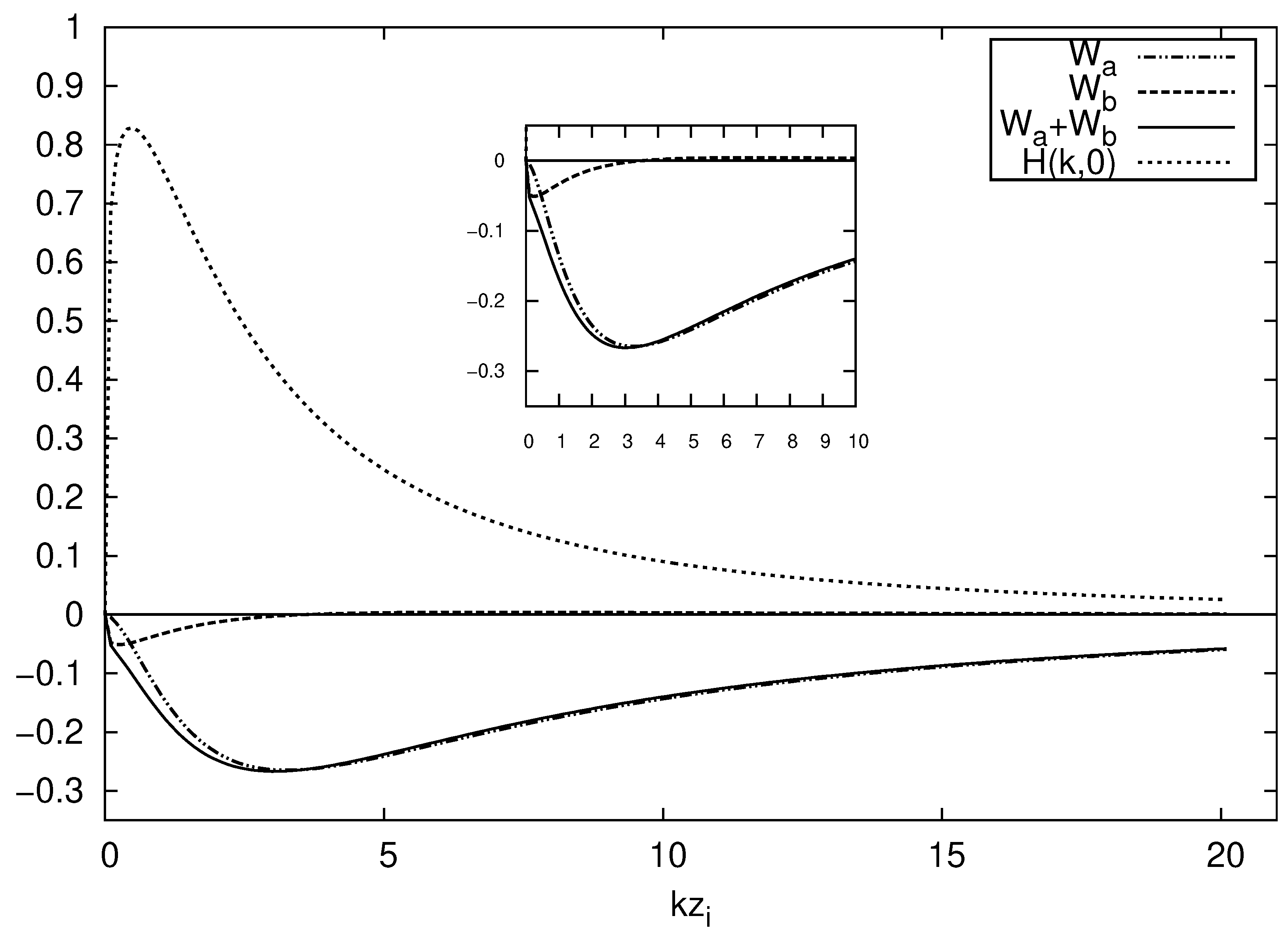
- The first region corresponds to the low number of waves (low-frequency) is divided into two parts. In general, the range that starts close to zero to does not contain most of the total turbulent energy. However, this is where the entrance of energy through mechanical sources occurs (denoted ) by the mean wind shear and thermal sources (denoted ), which produce thermal instability. In it, eddies are anisotropic and their properties depend on how they were generated. In addition, the largest eddies interact with the contours and layer of inversion of Planetary Boundary Layer (PBL) in this region. Nevertheless, the presence of the most energetic eddies is verified by the interval and, thus, these eddies contain the largest portion of the total TKE;
- The second region is called the inertial subinterval and corresponds to the range of the wave numbers to , being the turbulence isotropic or close to the isotropic condition. In this interval energy, it is neither generated nor consumed, it is only transferred from large to small eddies at a rate per unit mass. This highlights the performance of a TKE transfer mechanism, noted by , in the turbulent flow. The turbulence in this interval is stationary and entirely determined by rate [31], terefore one can apply the law of Kolmogorov to describe the STKE in this range and given by:
- The third region corresponds to high wave numbers (high-frequency), where the viscous forces of molecular origin dissipate TKE in the form of heat.
2.2. Model Evolution for the STKE in CBL
2.2.1. Thermal Convection
2.2.2. Mechanical Energy Production
2.2.3. Kinetic Energy Transfer by Inertial Effect
2.2.4. Energy Dissipation by Molecular Viscosity and Time Variation of the STKE: Dimensionless Equations
2.3. The Evolution Equation for Dimensionless STKE
2.4. First Order Linear PDEs
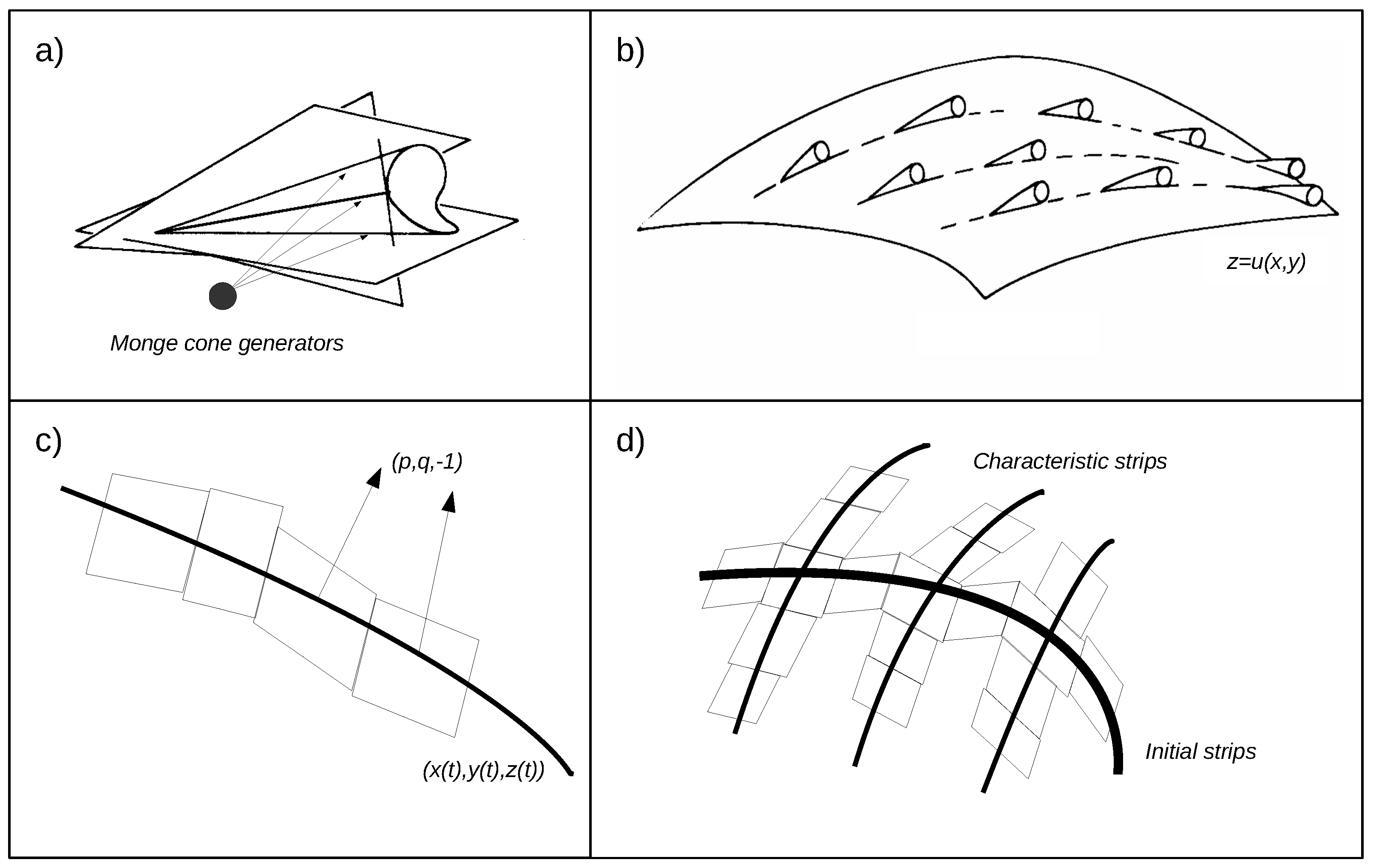
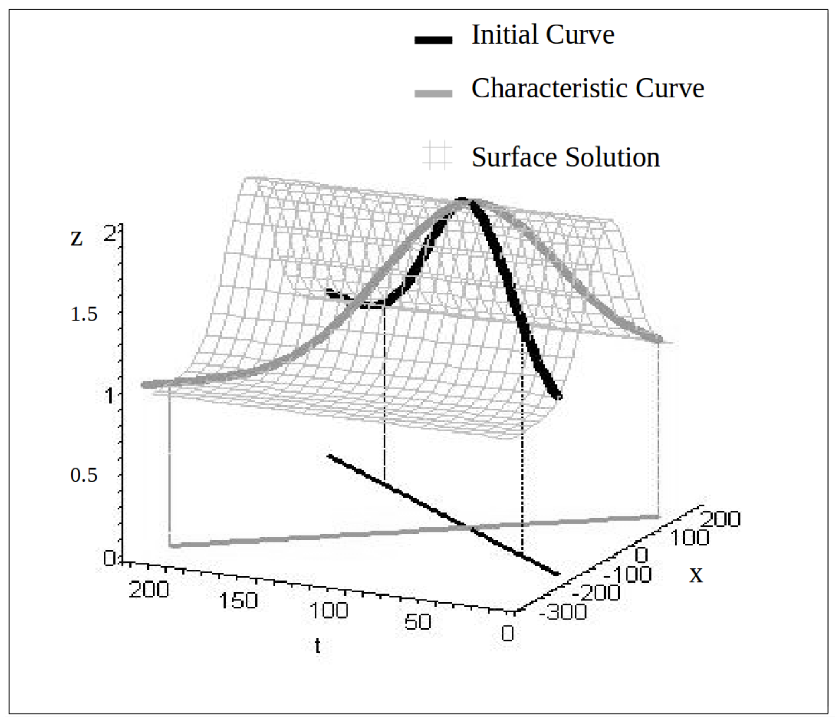
2.4.1. Method of Characteristics
2.4.2. Local Existence and Uniqueness of Solution for a Linear First Order PDE
- i.
- satisfies IC: . Indeed, , where for the purposes of simplifying notation, it is assumed that ;
- ii.
- around , given , one haswith the initial condition given by:Thus, if the characteristic curve has a point in common with the integral surface, the entire curve will be contained in it;
- iii.
- Given , according to the Chain Rule, we obtain:The matrix associated with this system is the Jacobian Matrix itself: , which has non-zero determinant due to its Non-Characteristic Condition. Thus, the above System has a unique solution;
- iv.
- From the second equation of System (35), we have: .Naming , there is a System of ODEs synthesized bywhose solution is .Note that the associated initial condition is given by: , therefore and unique. With this,Since is a solution of this System (for the same reasons as System (37)), it follows that is for .
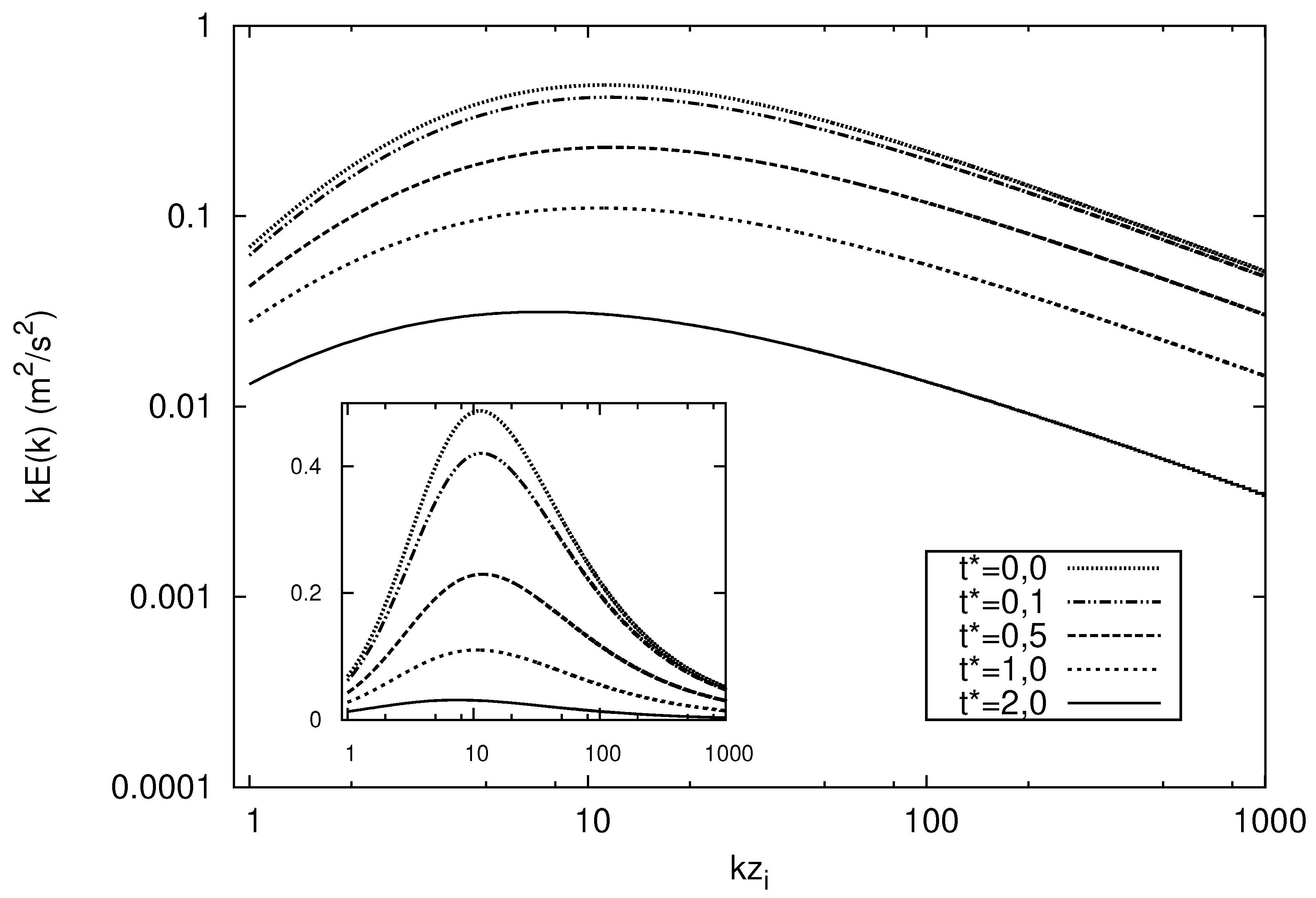
3. Isotropic Model
4. Final Considerations
Author Contributions
Funding
Acknowledgments
Conflicts of Interest
Abbreviations
| STKE | Spectral Density Turbulent Kinetic Energy Equation |
| TKE | Turbulent Kinetic Energy |
| CBL | Convective Boundary Layer |
| 3D-STKE | Three-Dimensional Energy Spectrum |
| PDE | Partial Differential Equation |
| PBL | Planetary Boundary Layer |
| 1L-PDE | Linear First Order Partial Differential Equation |
| 1st-PDE | First Order Partial Differential Equation |
| ODE | Ordinary Differential Equation |
| IC | Initial Condition |
| IVP | Initial Value Problem |
Appendix A


Non-Characteristic Condition
- i.
- The initial curve is a characteristic curve.In this case, , and considering the solution of the system: is given by .In order to obtain the bijection, we solve r and s as a function of , although the system does not allow this inversion. From it we only obtain that , and then Additionally, if is constant, there are inumerous solutions to the problem. If IC: , with non-constant f the problem does not admit solution [7].
- ii.
- If with tangent vectors parallel to the tangent vectors of the projected characteristic curve.Let, IC . At the tangent vectors of the characteristic curve and the initial curve are parallel. In this situation, a solution is obtained for r and for s, in the form: and , since .
Appendix B. Parameterization Employed in the Construction of Three-Dimensional Spectrum
- is the height above the ground and is the top of the CBL and n is the frequency;
- is the reduced frequency and is the average horizontal wind speed;
- is the convective velocity scale and is the surface friction velocity;

References
- Hinze, J.O. Turbulence; Mc Graw Hill: New York, NY, USA, 1975; p. 790. [Google Scholar]
- Tennekes, H.; Lumley, J.K. A First Course in Turbulence; The MIT Press: Cambridge, MA, USA, 1972; p. 301. [Google Scholar]
- Kristensen, L.; Lenschow, D.; Kirkegaard, P.; Courtney, M. The spectral velocity tensor for homogeneous boundary-layer turbulence. Bound.-Layer Meteorol. 1989, 47, 149–193. [Google Scholar] [CrossRef]
- Szinvelski, C.R.P. Uma Solução Para a Equação da Energia Cinética Turbulenta Empregando o Método das Características. Ph.D. Thesis, Universidade Federal de Santa Maria, Santa Maria, Brazil, 2009. [Google Scholar]
- Goulart, A.G.O. Desenvolvimento de um Modelo Espectral para o Estudo do Decaimento da Turbulência na Camada Limite Convectiva. Ph.D. Thesis, Universidade Federal De Santa Maria-UFSM, Santa Maria, Brazil, 2001. [Google Scholar]
- John, F. Partial Differential Equations, 2nd ed.; Sprienger-Verlag New York Inc.: New York, NY, USA, 1982; p. 259. [Google Scholar]
- Iório, V.M. EDP. Um Curso de Graduação, 2nd ed.; IMPA: Rio de Janeiro, Brazil, 2001; p. 300. [Google Scholar]
- Szinvelski, C.R.P.; Degrazia, G.A.; Goulart, A.G. Um modelo híbrido para evolução espectral da densidade de energia no período da manhã. Ciência Natura 2009. Edição Especial: VI Workshop Brasileiro de Micrometeorologia, 41–44. Available online: https://periodicos.ufsm.br/cienciaenatura/article/view/9512 (accessed on 20 September 2019).
- Degrazia, G.A.; Rizza, U.; Mangia, C.; Tirabassi, T. Validation of a new turbulent parameterization for dispersion models in convective conditions. Bound.-Layer Meteorol. 1997, 85, 243–254. [Google Scholar] [CrossRef]
- Folland, G.B. Introduction to Partial Differential Equations, 2nd ed.; Princeton Academic Press: Princeton, NJ, USA, 1995. [Google Scholar]
- Degrazia, G.A.; Buligon, L.; Szinvelski, C.R.P.; Moor, L.; Costa Acevedo, O. Uma revisão teórica sobre funções de Autocorrelação aplicadas a altas e baixas Velocidades do vento. Ciência Natura 2014, 36. [Google Scholar] [CrossRef]
- Taylor, G.I. Diffusition by continuous movements. Proc. Lond. Math. Soc. 1921, 20, 196–212. [Google Scholar]
- Tennekes, A.H. The exponential Lagrangian correlation function and turbulent diffusion in the inertial subrange. Atmos. Environ. 1979, 13, 1565–1568. [Google Scholar] [CrossRef]
- Batchelor, G.K. The Theory of Homogeneous Turbulence. The Theory of Homogeneous Turbulence; Cambridge University Press: Cambridge, UK, 1953. [Google Scholar]
- Degrazia, G.A.; Anfonssi, D.; Campos Velho, H.F.; Ferrero, E. A Lagrangian decorrelation time scale fin the Convective Boundary Layer. Bound.-Layer Meteorol. 1998, 86, 525–534. [Google Scholar] [CrossRef]
- Degrazia, G.A.; Anfonssi, D.; Carvalho, J.C.; Mangia, C.; Tirabassi, T.; Campos Velho, H.F. Turbulence parameterisation for PBL dispersion models in all stability conditions. Atmos. Environ. 2000, 34, 3575–3583. [Google Scholar] [CrossRef]
- Degrazia, G.A.; Moreira, D.M.; Vilhena, M.T. Derivation of an eddy diffusity depending on source distance for vertically inhomogeneous turbulence in a convective boundary layer. J. Appl. Meteorol. 2001, 40, 1233–1240. [Google Scholar] [CrossRef]
- Anfossi, D.; Oettl, D.; Degrazia, G.; Goulart, A. An analysis of sonic anemometer observations in low wind speed conditions. Bound.-Layer Meteorol. 2005, 114, 179–203. [Google Scholar] [CrossRef]
- Phillips, P.; Panofsky, H. A re-examination of lateral dispersion from continuous sources. Atmos. Environ. 1982, 16, 1851–1859. [Google Scholar] [CrossRef]
- Moor, L.; Degrazia, G.A.; Stefanello, M.B.; Mortarini, L.; Acevedo, O.C.; Maldaner, S.; Szinvelski, C.R.; Roberti, D.R.; Buligon, L.; Anfossi, D. Proposal of a new autocorrelation function in low wind speed conditions. Phys. A Stat. Mech. Appl. 2015, 438, 286–292. [Google Scholar] [CrossRef]
- Manomaiphiboon, K.; Russell, A.G. Evaluation of some proposed forms of Lagrangian velocity correlation coefficient. Int. J. Heat Fluid Flow 2003, 24, 709–712. [Google Scholar] [CrossRef]
- Szinvelski, C.R.; Buligon, L.; Stefanello, M.B.; Maldaner, S.; Roberti, D.R.; Degrazia, G.A. Testing Physical and Mathematical Criteria in a New Meandering Autocorrelation Function. In Turbulence Modelling Approaches-Current State, Development Prospects, Applications; IntechOpen: London, UK, 2017. [Google Scholar] [CrossRef]
- Gardiner, C.W. Handbook of Stochastic Methods for Physics, Chemistry and the Natural Sciences; Springer: Berlin, Germany, 1985; p. 442. [Google Scholar]
- Degrazia, G.A.; Goulart, A.G.O. Aplicações da Dinâmica de Fluidos em escoamentos na Camada Limite Planetária. Ciência e Natura 2005. Edição Especial, 10–57. Available online: https://repositorio.ufsm.br/bitstream/handle/1/2652/Guerra_Thiago.pdf?sequence=1&isAllowed=y (accessed on 20 September 201).
- Kaimal, J.C.; Wyngaard, D.A.; Haugen, D.A.; Coté, O.R.; Izumi, Y.; Caughey, S.J.; Readings, C.J. Turbulence structure in the Convective Boundary Layer. J. Atmos. Sci. 1976, 33, 2152–2226. [Google Scholar] [CrossRef]
- Yeh, T.; Atta, C. Spectral transfer of scalar and velocity fields in heated-grid turbulence. J. Fluid Mech. 1973, 58, 233–261. [Google Scholar] [CrossRef]
- Comte-Bellot, G.; Corrsin, S. The use of a contraction to improve the isotropy of grid-generated turbulence. J. Fluid Mech. 1966, 25, 657–682. [Google Scholar] [CrossRef]
- Buligon, L.; Szinvelski, C.R.P. Solução do Modelo de Pluma Gaussiana via Transformada de Fourier, 1st ed.; Gráfica Editora Pallotti: Santa Maria, Brazil, 2010; p. 240. [Google Scholar]
- Lumley, J.; Panofsky, H. The Structure of Atmospheric Turbulence; Interscience-Wiley: New York, NY, USA, 1964. [Google Scholar]
- McComb, W. The Physics of Fluid Turbulence; Clarendon Press: Oxford, UK, 1992. [Google Scholar]
- Kolmogorov, A.N. The local structure of turbulence in incompressible viscous fluid for large Reynolds number. Dokl. Akad. Nauk SSSR 1941, 30, 9–13. [Google Scholar] [CrossRef]
- Medeiros, L.E. Decaimento da Turbulência na Camada Superficial. Ph.D. Thesis, Universidade Federal De Santa Maria—UFSM, Santa Maria, Brazil, 2005. [Google Scholar]
- Stull, R.B. An Introduction to Boundary Layer Meteorology; Kluwer Academic Publishers: Dordrecht, The Netherlands, 1988; p. 666. [Google Scholar]
- Pao, Y. Structure of Turbulent Velocity and Scalar Fields at Large Wavenumbers. Phys. Fluids 1965, 8, 1063–1075. [Google Scholar] [CrossRef]
- Batchelor, G.K. Diffusion in a field of homogeneous turbulence, Eulerian analysis. Aust. J. Sci. Res. 1949, 2, 437–450. [Google Scholar] [CrossRef]
- Abentroth, R.A. Parametrização do Decaimento da turbulência na Camada Limite Convectiva. Ph.D. Thesis, Universidade Federal Do Rio Grande do Sul—UFRGS, Porto Alegre, Brazil, 2007. [Google Scholar]
- Nunes, A.B.; Campos Velho, H.F.; Satyamurty, P.; Degrazia, G.; Goulart, A.; Rizza, U. Morning Boundary-Layer Turbulent Kinetic Energy by Theoretical Models. Bound.-Layer Meteorol. 2009, 134, 23. [Google Scholar] [CrossRef]
- Goulart, A.G.; Moreira, D.M.; Vilhena, M.T.; Degrazia, G.A.; Zilitinkevich, S.S. A New Model for the CBL Growth Based on the Turbulent Kinetic Energy Equation. Environ. Fluid Mech. 2007, 007, 409–419. [Google Scholar] [CrossRef]
- Goulart, A.; Degrazia, G.A.; Rizza, U.; Anfossi, D. A Theorical Model for the Study of Convective Turbulence Decay and Comparison with Large-Eddy Simulation Data. Bound. Layer-Meteorol. 2003, 107, 143–155. [Google Scholar] [CrossRef]
- Sorbjan, Z. Decay of convective turbulence revisited. Bound.-Layer Meteorol. 1997, 82, 501–515. [Google Scholar] [CrossRef]
- Goulart, A.G.; de Vilhena, M.T.M.B.; Moreira, D.M.; Bodman, B.E.J. An Analytical Solution for the Nonlinear Spectrum Equation by the Decomposition Method. J. Phys. A 2008, 41, 8. [Google Scholar] [CrossRef]
- Degrazia, G.; Goulart, A.; Anfossi, D.; Campos Velho, H.; Lukaszcyk, P.; Palandi, J. A model based on Heisenberg’s theory for the eddy diffusivity in decaying turbulence applied to the residual layer. Nuovo Cimento-Soc. Ital. Fisica Sez. C 2003, 26, 39–52. [Google Scholar]
- Teschl, G. Ordinary Differential Equations and Dynamical Systems; American Mathematical Soc.: Providence, RI, USA, 2010; Volume 140. [Google Scholar]
- Doering, C.I.; Lopes, A.O. Equações Diferencias Ordinárias, 1st ed.; IMPA: Rio de Janeiro, Brazil, 2005; p. 421. [Google Scholar]
- Biezuner, R.J. Notas de Aula: Equações Diferenciais Parciais I/II. 2010. Disponível em. Available online: http://arquivoescolar.org/bitstream/arquivo-e/151/1/edp.pdf (accessed on 8 October 2019).
- Alonso, I.P. Primer Curso de Ecuaciones en Derivadas Parciales. Almeria, ES, 2005. p. 334. Available online: http://matematicas.uam.es/~ireneo.peral/libro.pdf (accessed on 8 October 2019).
- Evans, L.C. Partial Diferential Equations—Graduate Studies in Mathematics—Volume 19, 2nd ed.; Americam Mathematical Society: Providence, RI, USA, 2010; p. 662. [Google Scholar]
- Buligon, L.; Degrazia, G.; Szinvelski, C.; Goulart, A. Algebraic Formulation for the Dispersion Parameters in an Unstable Planetary Boundary Layer: Application in the Air Pollution Gaussian Model. Open Atmos. Sci. J. 2008, 2, 153–159. [Google Scholar] [CrossRef][Green Version]
- Goulart, A.G.; Vilhena, M.T.; Degrazia, G.A.; Flores, D.T. Vertical, lateral and longitudinal eddy diffusivities for a decaying turbulence in the convective boundary layer. Ecol. Model. 2007, 204, 516–522. [Google Scholar] [CrossRef]
- Goulart, A.G.; Degrazia, G.A.; Campos, C.; Silveira, C.P. Coeficientes de difusão turbulentos para a camada residual. Rev. Bras. De Meteorol. 2004, 19, 123–128. [Google Scholar]
- Moeng, C.; Sullivan, P. Evaluation of Turbulent Transport and Dissipation Closures in Second-Order Modeling. J. Atmos. Sci. 1989, 46, 2311–2330. [Google Scholar] [CrossRef]
- Levandosky, J. Math 220A. Partial Differential Equations of Applied Mathematics. Stanford, CA, USA, 2002. Disponível em. Available online: http://www.stanford.edu/class/math220a/handouts/firstorder.pdf (accessed on 8 October 2019).
- Lima, E.L. Curso de Análise Volume 2, 6th ed.; Instituto de Matemática Pura e Aplicada: Rio de Janeiro, Brazil, 2000; p. 557. [Google Scholar]
- Champagne, F.H.; Friehe, C.A.; Larve, J.C.; Wyngaard, J.C. Flux measurements, flux estimation techniques, and fine scale turbulence measurements in the instable surface layer over land. J. Atmos. Soc. 1977, 34, 515–520. [Google Scholar] [CrossRef]
- Sorbjan, Z. Structure of the Atmospheric Boundary Layer; Prentice Hall: Englewood Cliffs, NJ, USA, 1989; p. 317. [Google Scholar]
- Caughey, S.J.; Palmer, S.G. Some aspects of turbulence structure through the depth of the convective boundary layer. Q. J. R. Meteorol. Soc. 1979, 105, 811–827. [Google Scholar] [CrossRef]
- Hϕjstrup, J. Velocty spectra in the unstable surface planetary boundary layer. J. Atmos. Sci. 1982, 39, 2239–2248. [Google Scholar]
- Wilson, K. A three-dimensional correlation/spectral model for turbulent velocities in a convective boundary layer. Bound.-Layer Meteorol. 1997, 85, 35–52. [Google Scholar] [CrossRef]
- Moeng, C. A large-eddy-simulation model for the study of planetary boundary-layer turbulence. J. Atmos. Sci. 1984, 41, 2052–2062. [Google Scholar] [CrossRef]
- Caughey, S.J. Observed Characteristics of the Atmospheric Boundary Layer. In Atmospheric Turbulence and Air Pollution Modelling; Nieuwstdat, F.T.M., van Dop, H., Eds.; Springer: Dordrecht, The Netherlands, 1982; pp. 107–158. [Google Scholar] [CrossRef]
- Degrazia, G.A.; Anfonssi, D. Estimation of the Kolmogorov constant C0 from classical statistical diffusion theory. Atmos. Environ. 1998, 32, 3611–3614. [Google Scholar] [CrossRef]
- Moeng, C.; Sullivan, P. A comparison of shear-and buoyancy-driven planetary boundary layer flows. J. Atmos. Sci. 1994, 51, 999–1022. [Google Scholar] [CrossRef]
- Nieuwstadt, F.; Brost, R. The Decay of Convective Turbulence. J. Atmos. Sci. 1986, 43, 532–546. [Google Scholar] [CrossRef]


© 2019 by the authors. Licensee MDPI, Basel, Switzerland. This article is an open access article distributed under the terms and conditions of the Creative Commons Attribution (CC BY) license (http://creativecommons.org/licenses/by/4.0/).
Share and Cite
Paveglio Szinvelski, C.R.; Buligon, L.; Annes Degrazia, G.; Tirabassi, T.; Costa Acevedo, O.; Roberti, D.R. Employing the Method of Characteristics to Obtain the Solution of Spectral Evolution of Turbulent Kinetic Energy Density Equation in an Isotropic Flow. Atmosphere 2019, 10, 612. https://doi.org/10.3390/atmos10100612
Paveglio Szinvelski CR, Buligon L, Annes Degrazia G, Tirabassi T, Costa Acevedo O, Roberti DR. Employing the Method of Characteristics to Obtain the Solution of Spectral Evolution of Turbulent Kinetic Energy Density Equation in an Isotropic Flow. Atmosphere. 2019; 10(10):612. https://doi.org/10.3390/atmos10100612
Chicago/Turabian StylePaveglio Szinvelski, Charles Rogério, Lidiane Buligon, Gervásio Annes Degrazia, Tiziano Tirabassi, Otavio Costa Acevedo, and Débora Regina Roberti. 2019. "Employing the Method of Characteristics to Obtain the Solution of Spectral Evolution of Turbulent Kinetic Energy Density Equation in an Isotropic Flow" Atmosphere 10, no. 10: 612. https://doi.org/10.3390/atmos10100612
APA StylePaveglio Szinvelski, C. R., Buligon, L., Annes Degrazia, G., Tirabassi, T., Costa Acevedo, O., & Roberti, D. R. (2019). Employing the Method of Characteristics to Obtain the Solution of Spectral Evolution of Turbulent Kinetic Energy Density Equation in an Isotropic Flow. Atmosphere, 10(10), 612. https://doi.org/10.3390/atmos10100612