Downscaling Precipitation in the Data-Scarce Inland River Basin of Northwest China Based on Earth System Data Products

Abstract

Precipitation is a key climatic variable that connects the processes of atmosphere and land surface, and it plays a leading role in the water cycle. However, the vast area of Northwest China, its complex geographical environment, and its scarce observation data make it difficult to deeply understand the temporal and spatial variation of precipitation. This paper establishes a statistical downscaling model to downscale the monthly precipitation in the inland river basin of Northwest China with the Tarim River Basin (TRB) as a typical representation. This method combines polynomial regression and machine learning, and it uses the batch gradient descent (BGD) algorithm to train the regression model. We downscale the monthly precipitation and obtain a dataset from January 2001 to December 2017 with a spatial resolution of 1 km × 1 km. The results show that the downscaling model presents a good performance in precipitation simulation with a high resolution, and it is more effective than ordinary polynomial regression. We also investigate the temporal and spatial variations of precipitation in the TRB based on the downscaling dataset. Analyses illustrate that the annual precipitation in the southern foothills of the Tianshan Mountains and the North Kunlun Mountains showed a significant upward trend during the study periods, while the annual precipitation in the central plains presented a significant downward trend.

1. Introduction

Precipitation is a crucial part of the water and energy cycle [1,2]. As an important indicator of climate change and hydrological processes, changes in precipitation will inevitably affect the distribution of water resources in the river basins [3,4]. The variations of precipitation and its impacts on ecosystems have gradually become crucial issues in hydrology and ecology, especially in Northwest China [5]. The ecosystems based on the supply of precipitation and meltwater in the arid regions of Northwest China are more vulnerable under global warming [6,7,8]. Northwest China is rich in natural resources with an extremely vulnerable ecological environment due to its limited water resources [6,7]. Under the background of global warming, the climate change in Northwest China has presented a warm-wet trend during the past decades [4,6,9]. The significant increases in precipitation are mainly due to the increases in summer precipitation. Precipitation has a significant effect on regional climate change [2,10,11]. Consequently, it is critical to understand the temporal and spatial variation of precipitation.

However, traditional precipitation data usually come from meteorological stations and rely heavily on observation data [12]. A complex geographical environment, limited meteorological stations, and sparse observation data have made it hard to further investigate the variation of precipitation in Northwest China [2,12]. High mountains and basins widely distribute in Northwest China, which constitutes this particular natural unit with characteristics of the three significant ecosystems of mountain, oasis, and desert [13]. Its vast area, complicated geographical environment, and rare observation data make it difficult for people to deeply understand the temporal and spatial variation of precipitation of the data-scarce inland river basins in Northwest China. For the data-scarce inland river basins in Northwest China with complicated terrain and sparse meteorological stations, it is convenient to obtain precipitation data from Earth system data products [12]. The Tropical Rainfall Measuring Mission (TRMM)—a joint mission of NASA (National Aeronautics and Space Administration) and JAXA (Japanese Aerospace Exploration Agency) which was launched in 1997 to study precipitation and climate change—has good research potential [14,15]. TRMM Multi-Satellite Precipitation Analysis (TMPA, 3B43 V.7) is a new dataset that can accurately estimate precipitation distribution. The TMPA data could adequately capture the change of precipitation at the regional scale and have good correlation with the rain gauge data in China [16]. Compared with other versions of the dataset, TMPA performs better in the arid regions of Northwest China. Its long-term average annual precipitation produces a reasonable spatial distribution, and its average monthly precipitation trend is reasonable [17,18,19,20,21]. However, when applied to hydrological research in river basins, TMPA data still require downscaling to achieve a high resolution.

Downscaling methods are the universal solutions to address the problems of a low resolution. Conventional methods include linear regression, polynomial regression, and other machine learning methods [22,23,24,25,26]. Previous studies have established the relationships between precipitation, the normalized difference vegetation index (NDVI), and topography information by linear regression or polynomial regression to achieve downscaling precipitation [18,25,26,27,28]. However, the relationships between precipitation and topography information are not just linear, especially in Northwest China [12,25,29]. The downscaling results of Heihe river basin of Northwest China suggested that the downscaling simulation of quadratic polynomial regression is closer to the observed precipitation [25]. However, the downscaling methods of polynomial regression are based on normal equation methods, such as the least-squares method. The least-squares method is sensitive to noise and suitable for relatively small samples [30,31]. Gradient descent algorithms are often used as the core methods of training algorithms in the field of machine learning, and they is commonly used to recursively approximate a minimum deviation model, such as regression and artificial neural networks [32,33,34,35,36,37]. The batch gradient descent (BGD) algorithm is a conventional method of gradient descent that is widely used in the field of machine learning [35,38,39,40]. This algorithm can move towards the minimum value of cost function, and it is relatively stable, less affected by noise, and suitable for large samples [41,42].

In order to investigate the temporal and spatial variation of precipitation in the data-scarce river basin of Northwest China, this paper establishes a statistical downscaling method based on polynomial regression and BGD algorithm to simulate the spatial variation of monthly precipitation with a high resolution (1 km × 1 km). We selected the Tarim River Basin (TRB) as a typical representation of a data-scarce river basin in Northwest China. Based on the TMPA, NDVI, and DEM (Digital Elevation Model) data, we established a quadratic polynomial regression model of precipitation, DEM, the NDVI, aspect, and slope. We trained the regression model through the BGD algorithm (BGD-based polynomial regression) to downscale the monthly precipitation with a high spatial resolution (1 km × 1 km) from January 2001 to December 2017 and investigate the change in precipitation. Moreover, we compared the results of this statistical downscaling model and ordinary polynomial regression with the observation data and TMPA, respectively. This study improves the previous downscaling methods based on polynomial regression and enhances the downscaling accuracy, which will be helpful for future research about climate change and the downscaling of Northwest China.

2. Study Area and Materials

2.1. Description of the Study Area

The TRB is the most vast inland river basin in Northwest China (Figure 1), with a total area of about 1.02 × 10⁶ km² [13,43]. Due to extreme climate drought and limited water resources, the main source of water in the river basin is glacial snowmelt and precipitation [1,44]. The TRB is a closed river basin with unique water cycle processes which has a large temporal and spatial differences in precipitation distribution [2,45]. It is surrounded by high mountains, like the Tianshan Mountains, the Pamirs, the Karakorum Mountains, the Kunlun Mountains, and the Altun Mountains [46]. The middle region distributes the Taklimakan Desert. The complicated geographical environments of the TRB generate a closed basin with a typical continental climate [47].

2.2. Data Source

This paper mainly constructed the downscaling model of precipitation based on Earth system data products (topography, vegetation, and precipitation data), and it verified the downscaling simulation results with observation data. We used the TRMM Multi-Satellite Precipitation Analysis data (TMPA, 3B43 V.7) from January 2001 to December 2018 with a spatial resolution of 0.25° × 0.25°. Its units are in mm/hr, which we needed to convert to mm/month. (https://pmm.nasa.gov/TRMM). The NDVI data came from the MOD13A3 (Moderate-Resolution Imaging Spectroradiometer, Product ID: MOD13A3) NDVI monthly data with a spatial resolution of 1 km × 1 km and were provided by NASA Terra satellite. The time range of the NDVI was from January 2001 to December 2018 (https://lpdaac.usgs.gov/). The data, such as radiation correction, atmospheric correction, and geometric correction, were preprocessed by the data provider. To easily reflect the vegetation changes and process data, we needed to convert the projection to the World Geodetic System 1984 and splice the data from subregions by the row number. This research used the Global Bathymetry and Elevation Data at 30 Arc Seconds Resolution of SRTM (Shuttle Radar Topography Mission) DEM (https://topex.ucsd.edu/WWW_html/srtm30_plus.html). The data were developed by the Scripps Institute of Oceanography, University of California, San Diego. Their grid resolution was 30 seconds, which was about 1 km. Moreover, the aspect and slope were generated by the DEM. To verify the effectiveness of predicted precipitation, we also used the observation data of precipitation from January 2001 to December 2012 at ten stations in the TRB. The observation data of precipitation were downloaded from the Nation Meteorological Information Center (NMIC) (http://data.cma.cn/).

3. Methods

Firstly, we fit the quadratic polynomial regression of precipitation, DEM, the NDVI, aspect, and slope based on Earth system data products from January 2001 to December 2017. Secondly, we trained the regression through the BGD algorithm of machine learning. Then, we established a statistical downscaling model to downscale the monthly precipitation with a high resolution (1 km × 1 km) from January 2001 to December 2017 in the TRB. Based on the observation data of precipitation, we evaluated the downscaling results by calculating the correlation coefficient, the determination coefficient, the root mean square error, the mean absolute error, and the normalized mean square error [48,49,50,51]. Finally, we used the Mann-Kendall test to examine the variation of precipitation in the TRB during the past 17 years (Figure 2). The quantities of these methods are defined below in Section 3.3.

3.1. The BGD-Based Polynomial Regression

Precipitation alters the growth of vegetation, and vegetation can influence precipitation variation through seasonal variations [52,53]. Furthermore, precipitation is impacted by terrain, especially in mountains areas [12]. Bringing vegetation variation and terrain information into the downscaling simulation of monthly precipitation could be useful [54]. In this research, we used the DEM, aspect, and slope to represent the regional terrain information, and we used the NDVI to show the regional vegetation variation. We constructed a quadratic polynomial regression model based on the DEM, the NDVI, aspect, slope, and TMPA data to train the regression through the BGD algorithm to build the downscaling model. The downscaling model can be expressed as follows:

$$P=F\left(X,Y,Z,K\right)+\mathrm{\Delta }P,$$

(1)

where $F\left(X,Y,Z,K\right)$ represents the estimated values of quadratic polynomial regression, X is DEM, Y is the NDVI, Z is the aspect, and K is the slope. $\mathrm{\Delta }P$ (mm) is the residuals of the precipitation distribution caused by topography and vegetation factors. The cost function of linear regression is:

$$J\left(\theta \right)=\frac{1}{2m}{{\displaystyle \sum }}_{i=1}^m{\left(h_{\theta }\left(x^{\left(i\right)}\right)-y^{\left(i\right)}\right)}^2,$$

(2)

where x⁽ⁱ⁾ represents the feature of the samples, y⁽ⁱ⁾ is the target value, and m is the number of the samples. We trained the dataset to minimize the cost function, which allows one to find the optimal solution and solve the parameter θ of $minJ\left(\theta \right)$.

The unconstrained optimization problem is the basis of optimization theory, and an iterative method is usually used to find its optimal solutions [41,55]. Classical numerical optimization algorithms such as the gradient descent and Newton methods can allow one to an optimal solution. The gradient descent methods are usually used as the core methods of training algorithms in machine learning to recursively approximate the minimum deviation model. The BGD algorithm is a gradient descent method which is widely used in machine learning. The BGD algorithm searches for the most significant decline of the cost function in each iteration until the change in the cost function is minimized and stabilized. It is different from the Stochastic gradient descent (SGD) algorithm. The SGD algorithm only updates the parameters for one sample and randomly optimizes the cost function on a specific training data so that the training speed is accelerated. However, a single sample does not represent the trend of the entire sample, and the training speed comes at the expense of accuracy [41]. In this paper, we applied the gradient descent method to minimize the cost function, which was needed to find the partial derivative of $J\left(\theta \right)$:

$$\frac{\partial }{\partial {\theta }_j}J\left(\theta \right)=\frac{1}{m}{\displaystyle \sum }_{i=1}^m\left(h_{\theta }\left(x^{\left(i\right)}\right)-y^{\left(i\right)}\right)x_j^{\left(i\right)}.$$

(3)

The updating function of θ is:

$${\theta }_j={\theta }_j-\alpha \frac{1}{m}{\displaystyle \sum }_{i=1}^m\left(h_{\theta }\left(x^{\left(i\right)}\right)-y^{\left(i\right)}\right)x_j^{\left(i\right)},$$

(4)

where α is the learning rate and m is the number of samples. The iterative updating of θ uses all samples; this is called the BGD algorithm. The BGD algorithm uses all samples in a data set when iteratively updating parameters. Its time complexity is O (n). To improve the convergence speed, we could scale the feature samples:

$$x_j^{\left(i\right)}=\frac{x_j^{\left(i\right)}-{\mu }_j}{S_j},$$

(5)

where ${\mu }_j$ is the average value of $x_j$ and $S_j$ is the standard deviation of the sample.

3.2. Specific Steps of the Downscaling Model

(1) We resampled the DEM, the NDVI, aspect, and slope data to a low resolution (LR) of 0.25° × 0.25°; then, the high resolution (HR) became 1 km × 1 km.

(2) Then, we fit the polynomial regression equations for the multi-year average monthly data at the low resolution (0.25°) based on the correlations between DEM_LR, NDVI_LR, aspect_LR, slope_LR, and TMPA_LR. The predictor variables were DEM_LR, NDVI_LR, aspect_LR, and slope_LR, and the response variable was TMPA_LR. The regression model was trained by the BGD algorithm to obtain the polynomial regression equation and the regression coefficients C_LR of the twelve months.

(3) Based on the dataset (at the low resolution) from January 2001 to December 2017, we calculated the estimated values P_LR of polynomial regression at a low resolution and subtracted the P_LR from the TMPA original data to obtain the residual $\mathrm{\Delta }{P}_{LR}$. Then, we resampled $\mathrm{\Delta }{P}_{LR}$ by the ordinary Kriging interpolation to the high resolution of 1 km × 1 km to get the $\mathrm{\Delta }{P}_{HR}$.

(4) Based on the dataset (at the high resolution) from January 2001 to December 2017, we used the DEM_HR, NDVI_HR, aspect_HR, and slope_HR as predictor data in polynomial regression at a high resolution to obtain the estimated values P_HR. As a result, the predicted precipitation could be calculated by the equation:

$$P=P_{HR}+\mathrm{\Delta }{P}_{HR}.$$

(6)

3.3. The Evaluation of Downscaling Simulation

Based on the monthly precipitation data of the meteorological stations, we calculated the correlation coefficient (R), the determination coefficient (R²), the root mean square error (RMSE), the mean absolute error (MAE), and the normalized mean square error (NMSE) to evaluate the simulation results [49,50,56,57]. The methods are as follows:

$$R^2=1-\frac{{{\displaystyle \sum }}_{i=1}^n{\left(y_i-{\widehat{y}}_i\right)}^2}{{{\displaystyle \sum }}_{i=1}^n{\left(y_i-{\overline{y}}_i\right)}^2},$$

(7)

$$RMSE=\sqrt{\frac{{{\displaystyle \sum }}_{i=1}^n{\left(y_i-{\widehat{y}}_i\right)}^2}{N}},$$

(8)

$$MAE={{\displaystyle \sum }}_{i=1}^n\left|y_i-{\widehat{y}}_i\right|/N,$$

(9)

$$NMSE=\frac{\frac{1}{N}{{\displaystyle \sum }}_{i=1}^N{\left(y_i-{\widehat{y}}_i\right)}^2}{var\left(y\right)},$$

(10)

where $y_i$ is the observed value, ${\widehat{y}}_i$ is the predicted value, ${\overline{y}}_i$ is the average of observed value, and N is the number of samples.

3.4. Mann-Kendall Test

The Mann-Kendall test is a nonparametric test which can be used to examine the significance of the trend for climate hydrological time series [58,59]. This paper used the Mann-Kendall trend test to explore the trend of precipitation in the TRB of Northwest China. For a time series $Xt=\left(x_1,x_2,\dots ,x_n\right)$, the statistic S of the Mann-Kendall trend test can be calculated as follows:

$$S={\displaystyle \sum }_{i=1}^{n-1}{\displaystyle \sum }_{k=i+1}^{n}sgn\left(x_k-x_i\right).$$

(11)

For a set with a sample size greater than 8, the statistic S is close to a normal distribution with a mean value of 0, and its variances are:

$$Var\left(s\right)=\frac{n\left(n-1\right)\left(2n+5\right)-{{\displaystyle \sum }}_i{t}_i\left(t_i-1\right)\left(2t_i+5\right)}{18},$$

(12)

where $t_i$ is the number of i groups.

The calculation formula of the standardized statistic $Z_c$ is:

$$Z_c=\{\begin{array}{ll}\frac{S-1}{\sqrt{Var\left(S\right)}}& ,S>0\\ 0& ,S=0\\ \frac{S+1}{\sqrt{Var\left(S\right)}}& ,S<0\end{array},$$

(13)

where the $Z_c$ value is the trend statistics. Positive values indicate that the tested sequences show an increasing trend, and the negative values indicate a decreasing trend; if the absolute value of the $Z_c$ value is greater than the statistical value of 1.64 (95% confidence level—the 95% significant level indicates this test will erroneously detect significant trends 5% of the time), the trend of the sequences is significant.

The slope β is commonly used to measure the magnitude and direction of the variation trend, and its formula is:

$$\beta =Median\left(\frac{x_i-x_j}{i-j}\right),\forall j<i,$$

(14)

where 1 < j < i < n, and n is the number of the samples. When β > 0, there is an upward trend; otherwise, there is a downward trend. The absolute value of β represents the magnitude of the change.

4. Results

4.1. Downscaling Precipitation

Combining the supervised learning method and the cost function, we trained polynomial regression through the BGD algorithm to fit the regression equations with optimal parameters of 12 months from 2001 to 2017. We used the TMPA, DEM, NDVI, aspect, and slope at a 0.25° × 0.25° resolution as the training dataset. The testing dataset consisted of the DEM, NDVI, aspect, and slope, and it had the relatively high resolution of 1 km × 1 km. The initial learning rate of the algorithm α was 0.001, and the initial θ was a random value. The training results of the BGD algorithm are mapped in Figure 3. We compared the descent results at different learning rates within the limited iterations (Figure 3a), which indicates that the optimal learning rate α was equal to one. When α = 0.001 (initial learning rate) and α = 0.01, the cost function was hard to converge. When α = 0.1, the effectiveness of the convergence was unsatisfactory. When α = 1, the effectiveness of the convergence was relatively good. Consequently, we set the learning rate equal to 1. Moreover, we can see that the cost function continuously reduced and eventually stabilized after many iterations (Figure 3b). There were some differences in the relationships between cost function and iterations in each month. The cost functions of January, November, and December were relatively high, but they were relatively low in March, April, May, June, and July. This is because the relationship between vegetation and precipitation in summer and spring was more significant than in autumn and winter. Moreover, the increases in precipitation of the Northwest was mainly due to the variation of precipitation in summer and spring [11].

In order to verify the effectiveness of the downscaling model, we used the DEM, NDVI, slope, and aspect to downscale precipitation based on the 2018 dataset. We selected the observation data of four meteorological stations to test the significance of the downscaling results at different learning rates. We can conclude from Figure 4 and

Table 1. Validation of the downscaling model based on the observation data in 2018.

Meteorological Stations	Learning Rates	R	R2	RMSE	MAE	NMSE
Tazhong	0.001	0.6674 *	0.4454	4.4290	3.7167	0.5121
	0.01	0.7475 *	0.5587	4.1845	3.7584	0.4572
	0.1	0.7925 *	0.6280	3.7869	3.4501	0.3744
	1	0.8648 *	0.7470	2.9803	2.5185	0.2319
	1.2	0.8279 *	0.6854	3.4823	3.1418	0.3166
Tieganlik	0.001	0.7246	0.5251	5.0187	4.1417	0.4349
	0.01	0.7529	0.5668	4.3454	3.6417	0.4210
	0.1	0.7917	0.6268	3.6246	3.1250	0.3625
	1	0.9224 *	0.8012	2.5699	1.8721	0.1822
	1.2	0.8735	0.7630	3.4869	3.0667	0.3355
Yarkant	0.001	0.7590 *	0.5760	4.1774	3.2417	0.4140
	0.01	0.7988 *	0.6381	4.1333	3.1583	0.3519
	0.1	0.8604 *	0.7402	3.5451	2.7583	0.2360
	1	0.9326 *	0.8651	1.9327	1.4685	0.1236
	1.2	0.9218 *	0.8497	2.8875	2.4417	0.2760
Hotan	0.001	0.4001 *	0.1600	6.6599	4.5917	0.9540
	0.01	0.6284 *	0.3949	5.3728	3.7250	0.6209
	0.1	0.7317 *	0.5354	4.6860	2.8667	0.4723
	1	0.8938 *	0.7819	3.0488	2.2269	0.1999
	1.2	0.8168 *	0.6672	3.8255	3.0083	0.3148

Note: R is the correlation coefficient, R² is the determination coefficient, RMSE is the root mean square error, and MAE is the mean absolute error. The units of RMSE and MAE are mm. * represents a 0.01 significant level. NMSE is the normalized mean square error.

that the downscaling results were relatively optimal in the cases where the learning rate was equal to 1. The results showed that the trend of downscaling precipitation in 2018 was mainly consistent with the observation data (Figure 4). We can see that the four stations had relatively high precipitation in summer. Moreover, the downscaling data presented a good correlation with observation data at the learning rate of 1, with R in a range from 0.8648 to 0.9326, R² equal to 0.7470~0.8651, RMSE equal to 1.9327~3.0488, MAE equal to 1.4685~2.5185, and NMSE equal to 0.1236~0.2319; these values indicate that the downscaling model performed well in the downscaling simulation (Table 1). Consequently, we could continue to simulate precipitation with a high resolution

According to the validation of this downscaling model, the downscaling effectiveness was acceptable. Then, we used the DEM, NDVI, aspect, slope, and TMPA data from 2001 to 2017 to downscale the monthly precipitation based on BGD-based polynomial regression (the optimal parameters of BGD-based polynomial regression are provided in the Supplementary Materials).

4.2. Accuracy Test of Downscaling Results

In order to better evaluate the effect and accuracy of the downscaling model, we compared the downscaling results of polynomial regression and BGD-based polynomial regression with observation data and TMPA in 2001, respectively. On the other hand, we verified the downscaling precipitation from 2001 to 2017 of BGD-based polynomial regression by using the observation data.

4.2.1. Comparing the Downscaling Results of Ordinary Polynomial Regression and BGD-Based Polynomial Regression

In order to evaluate the effectiveness of the downscaling model, we downscaled the monthly precipitation in 2001 by using ordinary polynomial regression and BGD-based polynomial regression. Moreover, we also compared the downscaling results of these two methods with observation data and TMPA. Under the 0.01 significant level, TMPA had a good correlation with observation data in 2001, with R ranging from 0.7162 to 0.9789 and R² ranging from 0.5129 to 0.9000. Moreover, the downscaling model based on BGD-based polynomial regression performed better in the simulation than that based on ordinary polynomial regression. As shown in Figure 5 and

Table 2. Comparing the TRMM (Tropical Rainfall Measuring Mission) Multi-Satellite Precipitation Analysis (TMPA) and downscaling results based on observation data.

Meteorological Stations	Category	R	R2	RMSE	MAE	NMSE
Kumux	TMPA	0.7162 *	0.5129	3.8102	2.9245	0.4647
	PR	0.7192 *	0.5173	3.9872	3.2548	0.5089
	BGD	0.9763 *	0.9531	1.2257	0.9911	0.0481
Bayanbulak	TMPA	0.9394 *	0.8334	9.7502	7.0894	0.1527
	PR	0.8791 *	0.7727	21.7066	15.6610	0.7568
	BGD	0.9722 *	0.9264	6.4804	4.7365	0.0675
Korla	TMPA	0.8456 *	0.6406	1.4138	1.0941	0.3294
	PR	0.7669 *	0.5789	1.5303	1.1367	0.3860
	BGD	0.9871 *	0.9483	0.5363	0.4694	0.0474
Kalpin	TMPA	0.9415 *	0.8860	3.3912	2.3654	0.1045
	PR	0.7991 *	0.6385	8.1513	6.0004	0.6035
	BGD	0.9659 *	0.9239	2.7704	2.1234	0.0697
Alaer	TMPA	0.7262 *	0.5273	3.9437	2.1817	0.5797
	PR	0.7168 *	0.5139	3.8866	2.1003	0.5630
	BGD	0.9350 *	0.8365	2.0055	1.1281	0.1499
Tazhong	TMPA	0.7505 *	0.5632	1.4524	0.6817	0.4094
	PR	0.8056 *	0.6469	1.5500	1.2753	0.4663
	BGD	0.9722 *	0.9403	0.5311	0.2698	0.0547
Tieganlik	TMPA	0.9542 *	0.8339	0.3235	0.2131	0.1522
	PR	0.8016 *	0.6425	0.6717	0.6016	0.6563
	BGD	0.9765 *	0.9425	0.1904	0.1471	0.0527
Yarkant	TMPA	0.9682 *	0.9000	1.6390	1.3038	0.0917
	PR	0.7154 *	0.5118	3.7256	3.0942	0.4737
	BGD	0.9715 *	0.9438	1.6639	1.2537	0.0945
Pishan	TMPA	0.9789 *	0.8115	3.0822	2.2317	0.1773
	PR	0.8000 *	0.6399	4.5850	3.5451	0.3924
	BGD	0.9864 *	0.8066	3.0425	1.9604	0.1728
Hotan	TMPA	0.8630 *	0.7316	1.5303	1.0287	0.2460
	PR	0.7550 *	0.5700	2.0259	1.6649	0.4311
	BGD	0.9156 *	0.8217	1.2473	0.8306	0.1634

Note: TMPA is the precipitation at the low resolution of 0.25°, PR is the downscaling result of polynomial regression, and BGD is the downscaling result of BGD-based polynomial regression. R is the correlation coefficient, R² is the determination coefficient, RMSE is the root mean square error, and MAE is the mean absolute error. The units of RMSE and MAE are mm. * represents a 0.01 significant level. NMSE is the normalized mean square error.

, the results of the BGD-based polynomial regression showed similarly variation with observation data and TMPA, and they showed a higher correlation with the observation data than TMPA and ordinary polynomial regression, with R ranging from 0.9156 to 0.9871 and R² ranging from 0.8066 to 0.9531. The RMSE, MAE, and NMSE in Table 2 illustrate that the effectiveness of ordinary polynomial regression was relatively inadequate. The low RMSE (0.1904~6.4804), MAE (0.1471~4.7365), and NMSE (0.0474~0.1728) indicate that the effectiveness of BGD-based polynomial regression was acceptable.

4.2.2. The Accuracy Test for Downscaling Precipitation

In order to verify the downscaling results from 2001 to 2017, we extracted the downscaling precipitation of meteorological stations by the nearest neighbor method according to their locations. Then, we selected a total of 204 months of precipitation data (from January 2001 to December 2017) at each station for the verification of downscaling results, and we fit the scatter plots of calibration and validation between observation data and downscaling data. The calibration used the data of 2018, and the validation used the data from 2001 to 2017. The results of validation showed that there were good linear relationships between the downscaling data and observation data of the meteorological stations in the TRB, with R² ranging from 0.7243 to 0.9147 (Figure 6 and

Table 3. Accuracy test of downscaling precipitation from 2001 to 2017 based on observation data.

Meteorological Stations	R	R2	RMSE	MAE	NMSE
Kumux	0.8842 *	0.7243	3.8320	2.8080	0.2744
Bayanbulak	0.9506 *	0.8366	12.0196	8.1375	0.1626
Korla	0.9592 *	0.9147	2.9264	2.0685	0.0849
Kalpin	0.9088 *	0.8184	7.0488	4.7426	0.1807
Alaer	0.9035 *	0.7855	3.6482	2.4421	0.2135
Tazhong	0.8761 *	07421	2.8438	1.6513	0.2566
Tieganlik	0.9477 *	0.8957	2.2782	1.3692	0.1038
Yarkant	0.8958 *	0.7649	5.0749	2.7532	0.2339
Pishan	0.8660 *	0.7352	5.9348	3.6784	0.2635
Hotan	0.8878 *	0.7754	3.4006	2.3494	0.2235

Note: R is the correlation coefficient, R² is the determination coefficient, RMSE is the root mean square error, and MAE is the mean absolute error. The units of RMSE and MAE are mm. * represents 0.01 significant level. NMSE is the normalized mean square error.

). The correlation coefficients between the observation data and downscaling data of Kumux, Bayanbulak, Korla, Kalpin, Alaer, Tazhong, Tieganlik, Yarkant, Pishan, Hotan were 0.8842, 0.9506, 0.9592, 0.9088, 0.9035, 0.8761, 0.9477, 0.8958, 0.8660, and 0.8878, respectively. All these coefficients passed the 0.01 significant test, which illustrates that the downscaling data had a significant positive correlation with the observation data. Additionally, the RMSE, MAE, and NMSE of the downscaling data and observation data of each station revealed that the downscaling model had relatively good performance in the simulation. The validation results showed that the downscaling simulation had great accuracy.

Overall, the downscaling results were close to the observation data (Figure 7). The average, maximum, and minimum values were generally captured well in the downscaling simulation. However, there were still some outliers in the downscaling results (Figure 7a). Based on the comparison of monthly variation between downscaling results and observation data, we could see that these outliers were also present in the observation data, mainly in summer. The presentence of outliers in summer indicates the maximum in precipitation during the month, which was mainly due to the ununiform temporal variation of precipitation with high precipitation in summer and low precipitation in spring and winter [1,60]. Summer precipitation took over 50% of the total precipitation in the TRB, and the maximum precipitation in summer affect the overall annual precipitation in the TRB [2,8,61,62]. The downscaling model captured the precipitation extremes well, which means the very high and very low values were captured well in the downscaling results.

4.2.3. Comparing the Spatial Distribution of Downscaling Results and TMPA

This research input the DEM, NDVI, aspect, and slope data with a 1 km × 1 km resolution from January 2001 to December 2017 into the downscaling model. Based on the downscaling results, we obtained a monthly precipitation dataset with a high resolution (1 km × 1 km) from January 2001 to December 2017 in the TRB. As shown in Figure 8, we partly extracted the downscaling precipitation as a representation (April, August and December 2017) to compare with the original TMPA data of corresponding times. The spatial distribution of downscaling precipitation was consistent with the original TMPA data. The precipitation of TRB was mainly concentrated in the southern foothills of the Tianshan Mountains, and it was scarce in the central plains [1,2,60].

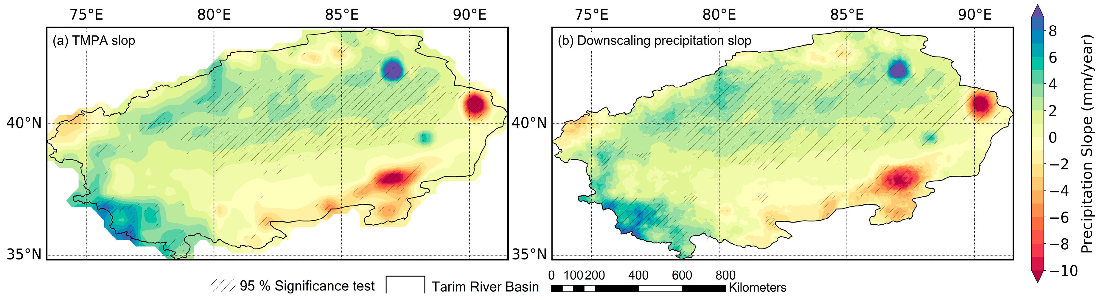
4.3. The Temporal and Spatial Variation of Precipitation

Based on the downscaling results, precipitation was mapped (Figure 9) to analyze its spatial distribution. We were able to illustrate that the precipitation in the TRB from 2001 to 2017 was mainly concentrated in the north and southwest mountainous, and it was scarce in the central and east plains (Figure 6). The spatial distribution characteristics of precipitation in the basin were similar to those of vegetation cover. [43,52]. The annual average maximum precipitation was about 411 mm, and the annual average precipitation reached about 110 mm.

The precipitation slope is mapped in Figure 10, which shows the variation of precipitation slope at the high resolution was consistent with the change at the low resolution. In the TRB, the areas where annual precipitation presented an increasing trend account for 72% of the total basins, and the overall variations of annual precipitation in this basin presented an upward trend. The increasing trend of annual precipitation was significantly high in the Kunlun Mountains and in the surrounding mountains of the South Tianshan Mountains. Additionally, the annual precipitation presented a more significant decline in Lop Nor and the North Altun Mountains than other areas. The increased amplitude of precipitation in the TRB from 2001 to 2017 decreased from the northwest to the southeast, with heavy precipitation in the northwest and southwest mountains and rare precipitation in the southeast. The results showed that the annual precipitation around the southern foothills of the Tianshan Mountains and the North Kunlun Mountains presented a significant upward trend, while the annual precipitation in the Lop Nor and the North Altun Mountains exhibited a significant downward trend (Figure 10).

5. Discussion

This paper established a statistical downscaling model based on BGD-based polynomial regression by simulating the relationship between the NDVI, DEM, aspect, slope, and precipitation. Based on the downscaling model, we downscaled the resolution of monthly precipitation in the TRB and investigated its temporal and spatial variation from 2001 to 2017. The cross-validations showed that the statistical downscaling model based on BGD-based polynomial regression could effectively downscale the monthly precipitation at a high resolution in the data-scarce inland river basin of Northwest China.

The learning rate impacted each iteration of the gradient descent algorithm. If the learning speed was too small, the algorithm needed more iterations to find the optimal parameters [42]. If the learning rate was too large, the algorithm probably missed the local minimum of cost function and resulted in an unsuccessful convergence. Usually choosing the appropriate learning rate α in the range of 0.001 ≤ α ≤ 10 [41,42]. We find the optimal learning rate of 1 after iterations and cross-validation. The BGD algorithm needed the updates of all parameters θ in each iteration, so the algorithm convergence was slow and the number of iterations was relatively large. On the other hand, the BGD algorithm could move towards the minimum value of cost function, and it was relatively stable. In this paper, polynomial regression was transformed into the form of linear regression. The cost function $J\left(\theta \right)$ of linear regression was a quadratic function with the global optimal solution. Therefore, training a regression model through the BGD algorithm could effectively minimize the cost function and find optimal parameters [39,41].

Quadratic polynomial regression could efficiently capture the information of precipitation that varied with terrain, consequently simulating the precipitation variation of complex terrain [12,25]. Constructing a downscaling model by fitting a linear regression model of the DEM, NDVI, and precipitation could simulate precipitation [27], while the relationships between precipitation, topographic factors, and vegetation were complicated in the areas with complex geographical environments [12,25]. We constructed a statistical downscaling model based on BGD-based polynomial regression to simulate monthly precipitation with a relatively high resolution in the TRB. In order to evaluate the effectiveness of the downscaling model, we compared the results of ordinary polynomial regression and BGD-based polynomial regression. The accuracy assessment of downscaling results in 2001 indicates that the BGD-based polynomial regression was more effective in the downscaling simulation. The reason for this is that ordinary polynomial regression was based on least-squares regression, but least squares regression was sensitive to noise [30,31]. The BGD algorithm can be used to solve least-squares problems, as it is less affected by noise and can be applied to large samples [41].

Moreover, the evaluations of downscaling precipitation from 2001 to 2017 showed that the downscaling precipitation based on this statistical downscaling model presented good linear relationships and significant correlations with the observation data. The RMSE, MAE, and NMSE of observation data and downscaling data were small, which illustrates that downscaling data were close to the observed data. The NMSE generally showed the most striking differences among models. If a model has a very low NMSE, then it is well-performing both in space and time [63,64]. Consequently, the NMSE (ranging from 0.0849 to 0.2744; Table 2) of the validation results indicate that the downscaling model performed well in the simulation.

Based on the downscaling precipitation model, precipitation in the TRB was mainly distribute in the mountains and was scarce in the plains. Precipitation was mostly concentrated in the South Tianshan Mountains and the Kunlun Mountains of this river basin, where there is relatively more coverage of vegetation [2,8,60,62]. The central plains had scarce precipitation. The spatial distribution of precipitation was consistent with the previous studies [5,65]. The annual precipitation in the TRB from 2001 to 2017 mainly showed an increasing trend, and the precipitation decreased from the northwest mountains to the southeast desert [2,66]. The upward variation of precipitation in the TRB is closely related to global warming and is deeply affected by the warm and humid climate change in the arid regions of Northwest China. This illustrates the responses of regional climate change to global warming [10,60].

However, there are still some uncertainties in the downscaling model. We used various earth system products from different satellites. The downscaling model can be impacted by atmospheric correction, data accuracy, and surface parameters [67,68,69,70]. Errors in observation instruments and data processing procedures could influence the model [71]. However, these uncertainties may be inevitable in the current technologies. To improve these issues, we can integrate and merge multiple data in later research to improve accuracy and reduce model uncertainty from data sources [72].

According to the accuracy test of the downscaling model, although the downscaling results had some deviations, their effectiveness was acceptable. We can conclude that the statistical downscaling model based on BGD-based polynomial regression can be used to simulate precipitation at a high resolution, and its downscaling result can be applied to investigate climate change in the inland river basins of Northwest China.

6. Conclusions

Based on earth system data products, this research established a statistical downscaling model by integrating polynomial regression and the BGD algorithm for the precipitation in the data-scarce inland river basins of Northwest China. We selected the TRB as a typical representation of the inland river basin of Northwest China, and we downscaled the monthly precipitation from January 2001 to December 2017 with a high resolution. The conclusions are as follows:

(1) The downscaling model based on BGD-based polynomial regression can efficiently downscale monthly precipitation with a high resolution in the data-scarce inland river basins of Northwest China. Based on this statistical downscaling model, we can effectively simulate precipitation at a high resolution (1 km × 1 km).

(2) The downscaling model based on BGD-based polynomial regression is more effective in the downscaling simulation than ordinary polynomial regression.

(3) Spatially, the precipitation from 2001 to 2017 was mainly concentrated in the surrounding mountains and was scarce in the central plains. Temporally, the variation of annual precipitation in the TRB presented a significant increasing trend during the study periods.

(4) Though we selected the TRB as a research target, the geographical environment conditions of the inland river basins in Northwest China are similar. Therefore, this statistical downscaling model can be used to simulate precipitation in other inland river basins of Northwest China.

References

1. Xu, Z.; Liu, Z.; Fu, G.; Chen, Y. Trends of major hydroclimatic variables in the Tarim River basin during the past 50 years. J. Arid Environ. 2010, 74, 256–267. [Google Scholar] [CrossRef]
2. Chen, Y.; Xu, C.; Hao, X.; Li, W.; Chen, Y.; Zhu, C.; Ye, Z. Fifty-year climate change and its effect on annual runoff in the Tarim River Basin, China. Quat. Int. 2009, 208, 53–61. (In Chinese) [Google Scholar] [CrossRef]
3. Chen, Y.; Takeuchi, K.; Xu, C.; Chen, Y.; Xu, Z. Regional climate change and its effects on river runoff in the Tarim Basin, China. Hydrol. Process. 2006, 20, 2207–2216. [Google Scholar] [CrossRef]
4. Zhang, Q.; Xu, C.; Tao, H.; Jiang, T.; Chen, Y.D. Climate changes and their impacts on water resources in the arid regions: A case study of the Tarim River basin, China. Stoch. Environ. Res. Risk Assess. 2009, 24, 349–358. [Google Scholar] [CrossRef]
5. Xu, J.; Chen, Y.; Li, W.; Liu, Z.; Tang, J.; Wei, C. Understanding temporal and spatial complexity of precipitation distribution in Xinjiang, China. Theor. Appl. Climatol. 2016, 123, 321–333. [Google Scholar] [CrossRef]
6. Xu, J.; Wang, C.; Li, W.; Zuo, J. Multi-temporal scale modeling on climatic-hydrological processes in data-scarce mountain basins of Northwest China. Arab. J. Geosci. 2018, 11, 423. [Google Scholar] [CrossRef]
7. Zhu, N.; Xu, J.; Li, W.; Li, K.; Zhou, C. A Comprehensive Approach to Assess the Hydrological Drought of Inland River Basin in Northwest China. Atmosphere 2018, 9, 370. [Google Scholar] [CrossRef]
8. Guo, P.W.; Zhang, X.K.; Shuyu, Z.Y.; Wang, C.L.; Zhang, X. Decadal variability of extreme precipitation days over Northwest China from 1963 to 2012. J. Meteorol. Res. 2014, 28, 1099–1113. [Google Scholar] [CrossRef]
9. Zuo, J.; Xu, J.; Li, W.; Yang, D. Understanding shallow soil moisture variation in the data-scarce area and its relationship with climate change by GLDAS data. PLoS ONE 2019, 14, e0217020. [Google Scholar] [CrossRef]
10. Shi, Y.F.; Shen, Y.P.; Kang, E.; Li, D.L.; Ding, Y.J.; Zhang, G.W.; Hu, R.J. Recent and future climate change in northwest china. Clim. Chang. 2007, 80, 379–393. [Google Scholar] [CrossRef]
11. Chen, Z. Quantitative Identification of River Runoff Change and Its Attribution in the Arid Region of Northwest China; East China Normal University: Shanghai, China, 2016. (In Chinese) [Google Scholar]
12. Wang, C.; Xu, J.; Chen, Y.; Bai, L.; Chen, Z. A hybrid model to assess the impact of climate variability on streamflow for an ungauged mountainous basin. Clim. Dyn. 2017, 50, 2829–2844. [Google Scholar] [CrossRef]
13. Zhao, R.; Chen, Y.; Zhou, H.; Li, Y.; Qian, Y.; Zhang, L. Assessment of wetland fragmentation in the Tarim River basin, western China. Environ. Geol. 2008, 57, 455–464. [Google Scholar] [CrossRef]
14. Huffman, G.J.; Bolvin, D.T.; Nelkin, E.J.; Wolff, D.B.; Adler, R.F.; Gu, G.; Hong, Y.; Bowman, K.P.; Stocker, E.F. The TRMM Multisatellite Precipitation Analysis (TMPA): Quasi-Global, Multiyear, Combined-Sensor Precipitation Estimates at Fine Scales. J. Hydrometeorol. 2007, 8, 38–55. [Google Scholar] [CrossRef]
15. Yong, B.; Liu, D.; Gourley, J.J.; Tian, Y.; Huffman, G.J.; Ren, L.; Hong, Y. Global View of Real-Time Trmm Multisatellite Precipitation Analysis: Implications for Its Successor Global Precipitation Measurement Mission. Bull. Am. Meteorol. Soc. 2015, 96, 283–296. [Google Scholar] [CrossRef]
16. Chen, F.; Gao, Y. Evaluation of precipitation trends from high-resolution satellite precipitation products over Mainland China. Clim. Dyn. 2018, 51, 3311–3331. [Google Scholar] [CrossRef]
17. Yang, Y.; Luo, Y. Evaluating the performance of remote sensing precipitation products CMORPH, PERSIANN, and TMPA, in the arid region of northwest China. Theor. Appl. Climatol. 2014, 118, 429–445. [Google Scholar] [CrossRef]
18. Zhang, Q.; Shi, P.; Singh, V.P.; Fan, K.; Huang, J. Spatial downscaling of TRMM-based precipitation data using vegetative response in Xinjiang, China. Int. J. Climatol. 2017, 37, 3895–3909. [Google Scholar] [CrossRef]
19. Adeyewa, Z.D.; Nakamura, K. Validation of TRMM Radar Rainfall Data over Major Climatic Regions in Africa. J. Appl. Meteorol. 2003, 42, 331–347. [Google Scholar] [CrossRef]
20. Franchito, S.H.; Rao, V.B.; Vasques, A.C.; Santo, C.M.E.; Conforte, J.C. Validation of TRMM precipitation radar monthly rainfall estimates over Brazil. J. Geophys. Res. 2009, 114. [Google Scholar] [CrossRef]
21. Karaseva, M.O.; Prakash, S.; Gairola, R.M. Validation of high-resolution TRMM-3B43 precipitation product using rain gauge measurements over Kyrgyzstan. Theor. Appl. Climatol. 2011, 108, 147–157. [Google Scholar] [CrossRef]
22. Ahmed, K.; Shahid, S.; Nawaz, N.; Khan, N. Modeling climate change impacts on precipitation in arid regions of Pakistan: A non-local model output statistics downscaling approach. Theor. Appl. Climatol. 2019, 137, 1347–1364. [Google Scholar] [CrossRef]
23. Sachindra, D.A.; Ahmed, K.; Rashid, M.M.; Shahid, S.; Perera, B.J.C. Statistical downscaling of precipitation using machine learning techniques. Atmos. Res. 2018, 212, 240–258. [Google Scholar] [CrossRef]
24. Sachindra, D.A.; Ahmed, K.; Shahid, S.; Perera, B.J.C. Cautionary note on the use of genetic programming in statistical downscaling. Int. J. Climatol. 2018, 38, 3449–3465. [Google Scholar] [CrossRef]
25. Fan, D.; Xue, H.; Dong, G.; Jiang, X.; Zhang, W.; Yin, H.; Guo, X. Downscaling Study on TRMM 3B43 Data of the Heihe River Basin Based on Quadratic Polynomial Regression Model. Res. Soil Water Conserv. 2017, 24, 146–151. (In Chinese) [Google Scholar] [CrossRef]
26. Fan, X.; Liu, H. Downscaling Method of TRMM Satellite Precipitation Data over the Tianshan Mountains. J. Nat. Resour. 2018, 33, 478–488. (In Chinese) [Google Scholar] [CrossRef]
27. Jia, S.; Zhu, W.; Lű, A.; Yan, T. A statistical spatial downscaling algorithm of TRMM precipitation based on NDVI and DEM in the Qaidam Basin of China. Remote Sens. Environ. 2011, 115, 3069–3079. [Google Scholar] [CrossRef]
28. Daly, C.; Neilson, R.P.; Phillips, D.L. A Statistical-Topographic Model for Mapping Climatological Precipitation over Mountainous Terrain. J. Appl. Meteorol. 1994, 33, 140–158. [Google Scholar] [CrossRef] [Green Version]
29. Wang, C.; Zhao, C. A Study of the Spatio-Temporal Distribution of Precipitation in Upper Reaches of Heihe River of China Using TRMM Data. J. Nat. Resour. 2013, 28, 862–872. (In Chinese) [Google Scholar] [CrossRef]
30. Knopov, P.; Kasitskaya, E. Consistency of least-square estimates for parameters of the Gaussian regression model. Cybern. Syst. Anal. 1999, 35, 19–25. [Google Scholar] [CrossRef]
31. Xu, W.; Chen, W.; Liang, Y. Feasibility study on the least square method for fitting non-Gaussian noise data. Phys. A Stat. Mech. Its Appl. 2018, 492, 1917–1930. [Google Scholar] [CrossRef] [Green Version]
32. Hu, T.; Wu, Q.; Zhou, D.X. Convergence of Gradient Descent for Minimum Error Entropy Principle in Linear Regression. IEEE Trans. Signal Process. 2016, 64, 6571–6579. [Google Scholar] [CrossRef]
33. Wang, J.; Wen, Y.; Gou, Y.; Ye, Z.; Chen, H. Fractional-order gradient descent learning of BP neural networks with Caputo derivative. Neural Netw. 2017, 89, 19–30. [Google Scholar] [CrossRef] [PubMed]
34. Chattopadhyay, S.; Chattopadhyay, G. Conjugate gradient descent learned ANN for Indian summer monsoon rainfall and efficiency assessment through Shannon-Fano coding. J. Atmos. Sol. Terr. Phys. 2018, 179, 202–205. [Google Scholar] [CrossRef]
35. Nakama, T. Theoretical analysis of batch and on-line training for gradient descent learning in neural networks. Neurocomputing 2009, 73, 151–159. [Google Scholar] [CrossRef]
36. Lee, C.-H. A gradient approach for value weighted classification learning in naive Bayes. Knowl. Based Syst. 2015, 85, 71–79. [Google Scholar] [CrossRef]
37. Kaoudi, Z.; Quiané-Ruiz, J.-A.; Thirumuruganathan, S.; Chawla, S.; Agrawal, D. A Cost-based Optimizer for Gradient Descent Optimization. arXiv 2017. [Google Scholar] [CrossRef]
38. Liu, Y.; Yang, D. Convergence analysis of the batch gradient-based neuro-fuzzy learning algorithm with smoothing L1/2 regularization for the first-order Takagi–Sugeno system. Fuzzy Sets Syst. 2017, 319, 28–49. [Google Scholar] [CrossRef]
39. Liu, Y.; Li, Z.; Yang, D.; Mohamed, K.S.; Wang, J.; Wu, W. Convergence of batch gradient learning algorithm with smoothing L1/2 regularization for Sigma–Pi–Sigma neural networks. Neurocomputing 2015, 151, 333–341. [Google Scholar] [CrossRef]
40. Shao, H.M.; Xu, D.P.; Zheng, G.F. Convergence of a Batch Gradient Algorithm with Adaptive Momentum for Neural Networks. Neural Process. Lett. 2011, 34, 221–228. [Google Scholar] [CrossRef]
41. Sun, Y.; Lin, W. Application of gradient descent method in machine learning. J. Suzhou Univ. Sci. Technol. 2018, 35, 26–31. (In Chinese) [Google Scholar] [CrossRef]
42. Ruder, S. An Overview of Gradient Descent Optimization Algorithms. 2017. Available online: https://arxiv.org/abs/1609.04747 (accessed on 9 October 2019).
43. Zhao, R.; Chen, Y.; Shi, P.; Zhang, L.; Pan, J.; Zhao, H. Land use and land cover change and driving mechanism in the arid inland river basin: A case study of Tarim River, Xinjiang, China. Environ. Earth Sci. 2012, 68, 591–604. [Google Scholar] [CrossRef]
44. Su, B.; Wang, A.; Wang, G.; Wang, Y.; Jiang, T. Spatiotemporal variations of soil moisture in the Tarim River basin, China. Int. J. Appl. Earth Obs. Geoinf. 2016, 48, 122–130. [Google Scholar] [CrossRef]
45. Lyu, J.; Shen, B.; Li, H. Dynamics of major hydro-climatic variables in the headwater catchment of the Tarim River Basin, Xinjiang, China. Quat. Int. 2015, 380–381, 143–148. [Google Scholar] [CrossRef]
46. Ling, H.; Xu, H.; Fu, J. Changes in intra-annual runoff and its response to climate change and human activities in the headstream areas of the Tarim River Basin, China. Quat. Int. 2014, 336, 158–170. [Google Scholar] [CrossRef]
47. Chen, Y.; Xu, C.; Chen, Y.; Liu, Y.; Li, W. Progress, challenges and prospects of eco-hydrological studies in the Tarim river basin of Xinjiang, China. Environ. Manag. 2013, 51, 138–153. [Google Scholar] [CrossRef]
48. Kendall, M.; Gibbons, J. Rank Correlation Method. Biometrika 1990, 11, 12. [Google Scholar] [CrossRef]
49. Shekhar, S.; Xiong, H. Root-Mean-Square Error. In Encyclopedia of GIS; Shekhar, S., Xiong, H., Eds.; Springer US: Boston, MA, USA, 2008; p. 979. [Google Scholar] [CrossRef]
50. Nahler, G. Pearson correlation coefficient. In Dictionary of Pharmaceutical Medicine; Nahler, G., Ed.; Springer Vienna: Vienna, Austria, 2009; p. 132. [Google Scholar] [CrossRef]
51. Poli, A.A.; Cirillo, M.C. On the use of the normalized mean square error in evaluating dispersion model performance. Atmos. Environ. Part A Gen. Top. 1993, 27, 2427–2434. [Google Scholar] [CrossRef]
52. Fang, J.; Piao, S.; Zhou, L.; He, J.; Wei, F.; Myneni, R.B.; Tucker, C.J.; Tan, K. Precipitation patterns alter growth of temperate vegetation. Geophys. Res. Lett. 2005, 32. [Google Scholar] [CrossRef] [Green Version]
53. Brunsell, N. Characterization of land-surface precipitation feedback regimes with remote sensing. Remote Sens. Environ. 2006, 100, 200–211. [Google Scholar] [CrossRef]
54. Wu, C.; Gonsamo, A.; Gough, C.M.; Chen, J.M.; Xu, S. Modeling growing season phenology in North American forests using seasonal mean vegetation indices from MODIS. Remote Sens. Environ. 2014, 147, 79–88. [Google Scholar] [CrossRef]
55. Sun, W.; Yuan, Y. Optimization Theory and Methods; Springer: Boston, MA, USA, 2006. [Google Scholar] [CrossRef]
56. Nagelkerke, N.J.D. A More General Definition of the Coefficient of Determination. Biometrika 1991, 78. [Google Scholar] [CrossRef]
57. Hassen, B.; Christian, A.G. Fast short-term global solar irradiance forecasting with wrapper mutual information. Renew. Energy 2019, 133, 1055–1065. [Google Scholar] [CrossRef]
58. Mann, H.B. Nonparametric Tests Against Trend. Econometrica 1945, 13, 245–259. [Google Scholar] [CrossRef]
59. Kossack, C.F.; Kendall, M.G. Rank Correlation Methods. Am. Math. Mon. 1950, 57, 425. [Google Scholar] [CrossRef]
60. Yang, P.; Xia, J.; Zhang, Y.; Hong, S. Temporal and spatial variations of precipitation in Northwest China during 1960–2013. Atmos. Res. 2017, 183, 283–295. [Google Scholar] [CrossRef]
61. Yan, G.; Lu, G.; Wu, Z. Analysis of Spatiotemporal Distribution of Precipitation in Tarim River Basin. Water Resour. Power 2009, 27, 1–3. (In Chinese) [Google Scholar] [CrossRef]
62. Mo, K.; Chen, Q.; Chen, C.; Zhang, J.; Wang, L.; Bao, Z. Spatiotemporal variation of correlation between vegetation cover and precipitation in an arid mountain-oasis river basin in northwest China. J. Hydrol. 2019, 574, 138–147. [Google Scholar] [CrossRef]
63. Singh, P.; Dwivedi, P. A novel hybrid model based on neural network and multi-objective optimization for effective load forecast. Energy 2019, 182, 606–622. [Google Scholar] [CrossRef]
64. Ferrero, E.; Oettl, D. An evaluation of a Lagrangian stochastic model for the assessment of odours. Atmos. Environ. 2019, 206, 237–246. [Google Scholar] [CrossRef]
65. Xu, J.; Chen, Y.; Lu, F.; Li, W.; Zhang, L.; Hong, Y. The Nonlinear trend of runoff and its response to climate change in the Aksu River, western China. Int. J. Climatol. 2011, 31, 687–695. [Google Scholar] [CrossRef]
66. Tao, H.; Gemmer, M.; Bai, Y.; Su, B.; Mao, W. Trends of streamflow in the Tarim River Basin during the past 50years: Human impact or climate change? J. Hydrol. 2011, 400, 1–9. [Google Scholar] [CrossRef]
67. Fensholt, R.; Proud, S.R. Evaluation of Earth Observation based global long term vegetation trends-Comparing GIMMS and MODIS global NDVI time series. Remote Sens. Environ. 2012, 119, 131–147. [Google Scholar] [CrossRef]
68. Brown, M.E.; Pinzon, J.E.; Didan, K.; Morisette, J.T.; Tucker, C.J. Evaluation of the consistency of long-term NDVI time series derived from AVHRR, SPOT-Vegetation, SeaWiFS, MODIS, and Landsat ETM+ sensors. IEEE Trans. Geosci. Remote Sens. 2006, 44, 1787–1793. [Google Scholar] [CrossRef]
69. Mukherjee, S.; Joshi, P.K.; Mukherjee, S.; Ghosh, A.; Garg, R.D.; Mukhopadhyay, A. Evaluation of vertical accuracy of open source Digital Elevation Model (DEM). Int. J. Appl. Earth Obs. Geoinf. 2013, 21, 205–217. [Google Scholar] [CrossRef]
70. Chen, J.; Brissette, F.P.; Leconte, R. Uncertainty of downscaling method in quantifying the impact of climate change on hydrology. J. Hydrol. 2011, 401, 190–202. [Google Scholar] [CrossRef]
71. Montanari, A.; Di Baldassarre, G. Data errors and hydrological modelling: The role of model structure to propagate observation uncertainty. Adv. Water Resour. 2013, 51, 498–504. [Google Scholar] [CrossRef]
72. Zhao, Y.; Huang, B.; Wang, C. Multi-temporal MODIS and Landsat reflectance fusion method based on super-resolution reconstruction. J. Remote Sens. 2013, 17, 590–608. (In Chinese) [Google Scholar] [CrossRef]
Figure 1. Study area locations of meteorological stations.
Atmosphere 10 00613 g001
Figure 2. The framework of the integrated model for downscaling precipitation.
Atmosphere 10 00613 g002
Figure 3. The relationship between cost function and iterations of batch gradient descent (BGD)-based polynomial regression. (a) The relationship between cost function and iterations under different learning rates. (b) The relationship between cost function and iterations in each month.
Atmosphere 10 00613 g003
Figure 4. The comparison of observation data and downscaling results of 2018. (ad) are the subgraphs of Tazhong, Tieganlik, Yarkant, Hotan.
Atmosphere 10 00613 g004
Figure 5. The comparison of the change in precipitation of 2001. (aj) are the variations of Kumux, Bayanbulak, Korla, Kalpin, Alaer, Tazhong, Tieganlik, Yarkant, Pishan, Hotan.
Atmosphere 10 00613 g005
Figure 6. The scatter plots of calibration and validation for the observation data and downscaling data of each meteorological station. (aj) are the scatter plots of Kumux, Bayanbulak, Korla, Kalpin, Alaer, Tazhong, Tieganlik, Yarkant, Pishan, Hotan.
Atmosphere 10 00613 g006
Figure 7. The outliers of precipitation from 2001 to 2017. (a) The boxplot of observation data and downscaling results for each station. (bk) present a comparison of the monthly precipitation between observation data and the downscaling of each station.
Atmosphere 10 00613 g007
Figure 8. The comparison of TMPA data (left) and downscaling precipitation (right). (a,c,e) represent the TMPA data of April, August, and December of 2017, respectively; (b,d,f) represent the downscaling precipitation of corresponding time.
Atmosphere 10 00613 g008
Figure 9. The spatial distribution of the annual average precipitation.
Atmosphere 10 00613 g009
Figure 10. The precipitation slope from 2001 to 2017. (a) Precipitation at the low resolution of 0.25°; (b) precipitation at the low resolution of 1 km.
Atmosphere 10 00613 g010