Inversion Models for the Retrieval of Total and Tropospheric NO₂ Columns

Abstract

Inversion models for retrieving the total and tropospheric nitrogen dioxide (${\mathrm{NO}}_2$) columns from spaceborne remote sensing data are presented. For total column retrieval, we propose the so-called differential radiance models with internal and external closure and solve the underlying nonlinear equations by using the method of Tikhonov regularization and the iteratively regularized Gauss–Newton method. For tropospheric column retrieval, we design a nonlinear and a linear model by using the results of the total column retrieval and the value of the stratospheric ${\mathrm{NO}}_2$ column delivered by a stratosphere–troposphere separation method. We also analyze the fundamentals of the commonly used differential optical absorption spectroscopy (DOAS) model and outline its relationship to the proposed inversion models. By a numerical analysis, we analyze the accuracy of the inversion models to retrieve total and tropospheric ${\mathrm{NO}}_2$ columns.

1. Introduction

Nitrogen dioxide (${\mathrm{NO}}_2$) is an important trace gas in the Earth’s stratosphere and troposphere. The stratospheric ${\mathrm{NO}}_2$ is strongly related to halogen compound reactions and ozone destruction [1]. In the troposphere, nitrogen oxides (NO_x = ${\mathrm{NO}}_2$ + NO) serve as a precursor of ozone in the presence of volatile organic compounds and a precursor of secondary aerosols through gas-to-particle conversion [2]. As a greenhouse gas, ${\mathrm{NO}}_2$ contributes significantly to radiative forcing locally [3]. As a prominent air pollutant affecting human health and ecosystems, substantial amounts of ${\mathrm{NO}}_2$ are produced in the boundary layer by industrial processes, power generation, transportation, and biomass burning.

Atmospheric remote sensing measurements in the UV and visible region, for instance, from nadir-viewing satellite instruments such as the Ozone Monitoring Instrument (OMI) [4] and Global Ozone Monitoring Experiment-2 (GOME-2) [5,6], have been monitoring global ${\mathrm{NO}}_2$ on a long-term scale. A new generation of instruments like the TROPOspheric Monitoring Instrument (TROPOMI) [7] aboard the Sentinel-5 Precursor satellite, with high spatial resolution, and geostationary missions like Sentinel-4 [8], with a fast revisit time, enable the continuous monitoring of ${\mathrm{NO}}_2$ concentrations for the following years. ${\mathrm{NO}}_2$ measurements from satellite instruments have been thoroughly validated using correlative ground-based measurements [9,10,11] and have been widely used to characterize the distribution, evolution, or transport of ${\mathrm{NO}}_2$ [12,13,14], to estimate ${\mathrm{NO}}_x$ emission [15,16], and to interpret ozone variation [17,18].

Based on a linearity assumption of the log of the radiances on the total column, the differential optical absorption spectroscopy (DOAS) model [19] is commonly used to derive the ${\mathrm{NO}}_2$ columns [20,21,22,23,24,25]. In DOAS, the spectral structure of a measured spectrum is separated into a narrowband absorption structure of trace gases and a broadband contribution approximated by a low-order polynomial. Effectively, the differential spectrum, used to obtain the trace gas information, is distinguished from the smooth background, such as Rayleigh scattering, cloud and aerosol extinction, and surface reflection.

In this paper, we aim to design inversion models that are more general than the DOAS model, for the retrieval of total and tropospheric ${\mathrm{NO}}_2$ columns. The underlying nonlinear equations of the inversion models are solved by using classical regularization methods. The paper is organized as follows. In Section 2, we describe the regularization methods for stably solving nonlinear ill-posed problems. In Section 3, we present two nonlinear inversion models for total ${\mathrm{NO}}_2$ column retrieval, while in Section 4, we design a nonlinear and a linear inversion model for tropospheric ${\mathrm{NO}}_2$ column retrieval. In Section 5, we analyze the theoretical basis of the DOAS model and outline its relationship to the general inversion models. The numerical accuracy of the proposed inversion models is investigated in Section 6.

2. Regularization Methods

In our analysis, we consider the nonlinear data model [26]

$${\mathbf{y}}^{\delta }=\mathbf{F}(\mathbf{x})+\mathbf{\delta },$$

(1)

where $\mathbf{F}:{\mathbb{R}}^n\to {\mathbb{R}}^m$ is the forward model, $\mathbf{x}\in {\mathbb{R}}^n$ is the state vector, ${\mathbf{y}}^{\delta }\in {\mathbb{R}}^m$ is the noisy data vector, and $\mathbf{\delta }\in {\mathbb{R}}^m$ is the measurement error vector. In a deterministic setting, the measurement error vector $\mathbf{\delta }$ is characterized by the noise level $\Delta$ (defined as an upper bound for $\mathbf{\delta }$, i.e., $\left|\right|\mathbf{\delta }\left|\right|\le \Delta$), the state vector $\mathbf{x}$ is a deterministic vector, and we are faced with the solution of the nonlinear equation

$${\mathbf{y}}^{\delta }=\mathbf{F}(\mathbf{x}).$$

(2)

In a stochastic setting, $\mathbf{\delta }$ and $\mathbf{x}$ are random vectors, and the data Model (1) is solved by means of a Bayesian approach.

Because the nonlinear Equation (2) is usually ill-posed, a regularization method should be used to compute a solution with physical meaning. In classical regularization theory, two widely used methods are the method of Tikhonov regularization and the iteratively regularized Gauss–Newton method.

2.1. Tikhonov Regularization

In the framework of Tikhonov regularization [27], a regularized solution to the nonlinear Equation (2) is computed as the minimizer of the Tikhonov function

$${\mathcal{F}}_{\alpha }(\mathbf{x})={∥{\mathbf{y}}^{\delta }-\mathbf{F}(\mathbf{x})∥}^2+\alpha {∥\mathbf{L}(\mathbf{x}-{\mathbf{x}}_{\mathrm{a}})∥}^2,$$

(3)

where $\alpha$ is the regularization parameter, $\mathbf{L}$ is the regularization matrix, and ${\mathbf{x}}_{\mathrm{a}}$ is the a priori state vector, the best beforehand estimate of the solution. The regularization matrix $\mathbf{L}$, controlling the magnitude or the smoothness of the solution, can be chosen as the identity matrix, a diagonal matrix, the discrete approximations to the first- and second-order derivative operators, or as the Cholesky factor of the inverse of an a priori covariance matrix.

The minimization of the Tikhonov function in Equation (3) can be formulated as a least-squares problem, and the regularized solution can be computed by using optimization methods, such as step-length and trust-region methods [28,29]. These nonlinear optimization methods are iterative methods, which compute the new iterate by approximating the objective function around the actual iterate by a quadratic model.

Belonging to the category of step-length methods, the Gauss–Newton method for least-squares problems has an important practical interpretation. At the iteration step i, considering a linearization of $\mathbf{F}(\mathbf{x})$ around the current iterate ${\mathbf{x}}_{\alpha i}^{\delta }$,

$$\mathbf{F}(\mathbf{x})\approx \mathbf{F}({\mathbf{x}}_{\alpha i}^{\delta })+{\mathbf{K}}_{\alpha i}(\mathbf{x}-{\mathbf{x}}_{\alpha i}^{\delta }),$$

(4)

where

$${\mathbf{K}}_{\alpha i}=\mathbf{K}({\mathbf{x}}_{\alpha i}^{\delta })=\frac{\partial \mathbf{F}}{\partial \mathbf{x}}({\mathbf{x}}_{\alpha i}^{\delta })\in {\mathbb{R}}^{m\times n}$$

(5)

is the Jacobian matrix evaluated at ${\mathbf{x}}_{\alpha i}^{\delta }$, and replacing $\mathbf{F}(\mathbf{x})$ in Equation (2) by its linearization (4), the result is

$${\mathbf{K}}_{\alpha i}(\mathbf{x}-{\mathbf{x}}_{\mathrm{a}})={\mathbf{y}}_i^{\delta },$$

(6)

where

$${\mathbf{y}}_i^{\delta }={\mathbf{y}}^{\delta }-\mathbf{F}({\mathbf{x}}_{\alpha i}^{\delta })+{\mathbf{K}}_{\alpha i}({\mathbf{x}}_{\alpha i}^{\delta }-{\mathbf{x}}_{\mathrm{a}})$$

(7)

is the linearized data vector at iteration step i. Since the nonlinear problem is ill-posed, its linearization is also ill-posed. Thus, we solve the linearized Equation (6) by means of Tikhonov regularization with the penalty term $\alpha \left|\right|\mathbf{L}(\mathbf{x}-{\mathbf{x}}_{\mathrm{a}}){\left|\right|}^2$.

The Tikhonov function for the linearized equation takes the form

$${\mathcal{F}}_{\mathrm{l}\alpha i}(\mathbf{x})={∥{\mathbf{y}}_i^{\delta }-{\mathbf{K}}_{\alpha i}(\mathbf{x}-{\mathbf{x}}_{\mathrm{a}})∥}^2+\alpha {∥\mathbf{L}(\mathbf{x}-{\mathbf{x}}_{\mathrm{a}})∥}^2,$$

(8)

and its minimizer, i.e., the new iterate ${\mathbf{x}}_{\alpha i+1}^{\delta }$, is given by

$${\mathbf{x}}_{\alpha i+1}^{\delta }={\mathbf{x}}_{\mathrm{a}}+{\mathbf{K}}_{\alpha i}^{†}{\mathbf{y}}_i^{\delta },$$

(9)

where

$${\mathbf{K}}_{\alpha i}^{†}={({\mathbf{K}}_{\alpha i}^T{\mathbf{K}}_{\alpha i}+\alpha {\mathbf{L}}^T\mathbf{L})}^{-1}{\mathbf{K}}_{\alpha i}^T$$

(10)

is the regularized generalized inverse, also known as the gain matrix [30], at iteration step i. The iterative process is stopped according to

• the relative X-convergence test [28], when the iterates ${\mathbf{x}}_{\alpha i}^{\delta }$ converge, and/or
• the relative function convergence test [30,31], when the residuals $\left|\right|{\mathbf{y}}^{\delta }-\mathbf{F}({\mathbf{x}}_{\alpha i}^{\delta })\left|\right|$ converge.

Therefore, the solution of a nonlinear ill-posed problem by means of Tikhonov regularization is equivalent to the solution of a sequence of ill-posed linearizations of the forward model about the current iterate.

The selection of the optimal value of the regularization parameter ${\alpha }_{\mathrm{opt}}$ is a crucial issue of Tikhonov regularization. With too little regularization, reconstructions deviate significantly from the a priori, and the solution is said to be underegularized. With too much regularization, the reconstructions are too close to the a priori, and the solution is said to be over-regularized. Several regularization parameter choice methods have been discussed in [26,32], including the expected error estimation method, the maximum likelihood estimation, generalized cross-validation [33], and the nonlinear L-curve method [34].

The idea of the expected error estimation method is to perform a random exploration of a domain, in which the exact solution ${\mathbf{x}}^{†}$ is supposed to lie, and for each state vector realization ${\mathbf{x}}_i^{†}$, to compute the optimal regularization parameter for error estimation as ${\alpha }_{\mathrm{opt}i}=arg{min}_{\alpha }\mathcal{E}\{||{\mathbf{e}}_{\alpha }^{\delta }({\mathbf{x}}_i^{†}){\left|\right|}^2\}$, where

$$\mathcal{E}\left\{{∥{\mathbf{e}}_{\alpha }^{\delta }({\mathbf{x}}^{†})∥}^2\right\}={∥{\mathbf{e}}_{\mathrm{s}\alpha }({\mathbf{x}}^{†})∥}^2+\mathcal{E}\{{∥{\mathbf{e}}_{\mathrm{n}\alpha }^{\delta }∥}^2$$

(11)

is the expected value of the total error vector ${\mathbf{e}}_{\alpha }^{\delta }({\mathbf{x}}^{†})={\mathbf{x}}^{†}-{\mathbf{x}}_{\alpha }^{\delta }$, ${\mathbf{e}}_{\mathrm{s}\alpha }({\mathbf{x}}^{†})=({\mathbf{I}}_n-{\mathbf{A}}_{\alpha })({\mathbf{x}}^{†}-{\mathbf{x}}_{\mathrm{a}})$ is the smoothing error vector, ${\mathbf{e}}_{\mathrm{n}\alpha }^{\delta }=-{\mathbf{K}}_{\alpha }^{†}\mathbf{\delta }$ is the noise error vector, ${\mathbf{x}}_{\alpha }^{\delta }$ is the regularized solution, and ${\mathbf{A}}_{\alpha }={\mathbf{K}}_{\alpha }^{†}{\mathbf{K}}_{\alpha }$ is the averaging kernel matrix at the solution ${\mathbf{x}}_{\alpha }^{\delta }$. Under the assumption that $\delta$ is white noise with variance ${\sigma }^2$, we compute the exponent $p_i=log{\alpha }_{\mathrm{opt}i}/log\sigma$ and choose the optimal regularization parameter as ${\alpha }_{\mathrm{opt}}={\sigma }^{\overline{p}}$, where $\overline{p}=(1/N_{\mathrm{x}}){\sum }_{i=1}^{N_{\mathrm{x}}}{p}_i$ is the sample mean exponent, and $N_{\mathrm{x}}$ is the sample size.

2.2. Iteratively Regularized Gauss–Newton Method

Unfortunately, at the present time, there is no fail-safe regularization parameter choice method that guarantees small solution errors in any circumstance, that is, for any noisy data vector. An amelioration of the problems associated with regularization parameter selection is achieved in the framework of the so-called iterative regularization methods, of which the iteratively regularized Gauss–Newton method [35] is a relevant representative. These approaches, in which the amount of regularization is gradually decreased during the iterative process, are less sensitive to overestimations of the regularization parameter but require more iteration steps to achieve convergence.

Essentially, the iteratively regularized Gauss–Newton method relies on the solution of the linearized equation (cf. Equation (6)) ${\mathbf{K}}_i(\mathbf{x}-{\mathbf{x}}_{\mathtt{a}})={\mathbf{y}}_i^{\delta }$ by means of Tikhonov regularization with the penalty term ${\alpha }_i\left|\right|\mathbf{L}(\mathbf{x}-{\mathbf{x}}_{\mathrm{a}}){\left|\right|}^2$. The new iterate minimizing the function

$${\mathcal{F}}_{\mathrm{l}i}(\mathbf{x})={∥{\mathbf{y}}_i^{\delta }-{\mathbf{K}}_i(\mathbf{x}-{\mathbf{x}}_{\mathrm{a}})∥}^2+{\alpha }_i{∥\mathbf{L}(\mathbf{x}-{\mathbf{x}}_{\mathrm{a}})∥}^2$$

(12)

is given by

$${\mathbf{x}}_{i+1}^{\delta }={\mathbf{x}}_{\mathrm{a}}+{\mathbf{K}}_i^{†}{\mathbf{y}}_i^{\delta },$$

(13)

where

$${\mathbf{K}}_i^{†}={({\mathbf{K}}_i^T{\mathbf{K}}_i+{\alpha }_i{\mathbf{L}}^T\mathbf{L})}^{-1}{\mathbf{K}}_i^T.$$

(14)

For iterative regularization methods, the number of iteration steps i plays the role of the regularization parameter, and the iterative process is stopped after an appropriate number of steps $i^{\star }$ in order to avoid an uncontrolled expansion of the errors in the data. In fact, a mere minimization of the residual $\left|\right|{\mathbf{r}}_i^{\delta }\left|\right|$, where

$${\mathbf{r}}_i^{\delta }={\mathbf{y}}^{\delta }-\mathbf{F}({\mathbf{x}}_i^{\delta })$$

is the residual vector at ${\mathbf{x}}_i^{\delta }$, leads to a semi-convergent behavior of the iterated solution: while the error in the residual decreases as the number of iteration steps increases, the error in the solution starts to increase after an initial decay.

A widely used a posteriori choice for the stopping index $i^{\star }$ in dependence of the noise level $\Delta$ is the discrepancy principle [36]. According to this stopping rule, the iterative process is terminated after $i^{\star }$ steps such that

$${∥{\mathbf{r}}_{i^{\star }}^{\delta }∥}^2\le \tau {\Delta }^2<{∥{\mathbf{r}}_i^{\delta }∥}^2,0\le i<i^{\star },$$

(15)

with $\tau >1$. Hence, the regularized solution of the iteratively regularized Gauss–Newton method is ${\mathbf{x}}_{i^{\star }}^{\delta }$. As in many practical problems arising in atmospheric remote sensing, the noise level cannot be a priori estimated, so we adopt a practical approach. This is based on the observation that the square residual $\left|\right|{\mathbf{r}}_i^{\delta }{\left|\right|}^2$ decreases during the iterative process and attains a plateau at approximately ${\Delta }^2$. Thus, if the nonlinear residuals $\left|\right|{\mathbf{r}}_i^{\delta }\left|\right|$ converge to $\left|\right|{\mathbf{r}}_{\infty }^{\delta }\left|\right|$ within a prescribed tolerance, we use the estimate

$${\Delta }^2=\left|\right|{\mathbf{r}}_{\infty }^{\delta }{\left|\right|}^2.$$

The above heuristic stopping rule does not have any mathematical justification but works sufficiently well in practice.

At first glance, this method seems to be identical to the method of Tikhonov regularization, but the following differences exist:

• the regularization parameters are the terms of a decreasing (geometric) sequence, i.e., ${\alpha }_i=q{\alpha }_{i-1}$, with $q<1$;
• the iterative process is stopped according to the discrepancy principle (15) instead of requiring the convergence of iterates.

The numerical experiments performed in [26] showed that at the solution ${\mathbf{x}}_{k^{\star }}^{\delta }$, ${\alpha }_{k^{\star }}$ is close to ${\alpha }_{\mathrm{opt}}$ and so that ${\mathbf{x}}_{k^{\star }}^{\delta }$ is close to the Tikhonov solution corresponding to the optimal value of the regularization parameter ${\mathbf{x}}_{{\alpha }_{\mathrm{opt}}}^{\delta }$. Another positive feature of the method is that by decreasing the regularization parameter at each iteration step, problems that do not require regularization (or a small amount of regularization) can be handled.

In the following, the method of Tikhonov regularization and the iteratively regularized Gauss–Newton method will be used to solve the nonlinear equations corresponding to different inversion models for total and tropospheric column retrievals.

3. Total NO₂ Column Retrieval

Consider a discretization of the atmosphere in $N_{\mathrm{lay}}$ layers, and let the stratosphere extend from layer 1 to layer $N_{\mathrm{t}}-1$ and the troposphere extend from layer $N_{\mathrm{t}}$ to layer $N_{\mathrm{lay}}$. The total column of a gas g is defined by

$$X_g=\sum _{j=1}^{N_{\mathrm{lay}}}{x}_{g,j},$$

(16)

while the stratospheric and tropospheric total columns are given respectively by

$$X_{\mathrm{s}g}=\sum _{j=1}^{N_{\mathrm{t}}-1}{x}_{g,j},$$

(17)

and

$$X_{\mathrm{t}g}=\sum _{j=N_{\mathrm{t}}}^{N_{\mathrm{lay}}}{x}_{g,j},$$

(18)

where $x_{g,j}$ is the partial column of gas g on later j. Obviously, we have $X_g=X_{\mathrm{t}g}+X_{\mathrm{s}g}$.

An important task of the retrieval is the computation of the partial derivative of the radiance I with respect to the total column $X_g$ of gas g. In a radiative transfer model, I is a function of $x_{g,j}$, i.e., $I=I(x_{g,1},\dots ,x_{g,N_{\mathrm{lay}}})$, and the partial derivatives $\partial I/\partial x_{g,j}$, $j=1,\dots ,N_{\mathrm{lay}}$ are computable quantities (delivered by a linearized radiative transfer model). Under the assumptions that the profile $\{x_{g,1},\dots ,x_{g,N_{\mathrm{lay}}}\}$ is a scaled version of an a priori profile $\{x_{\mathrm{a}g,1}\dots ,x_{\mathrm{a}g,N_{\mathrm{lay}}}\}$ and that $s_g$ is the scale factor of gas g, i.e., $x_{g,j}=s_g{x}_{\mathrm{a}g,j}$, for all $j=1,\dots ,N_{\mathrm{lay}}$, we have $s_g=X_g/X_{\mathrm{a}g}$ and hence the one-to-one correspondence $x_{g,j}=(X_g/X_{\mathrm{a}g})x_{\mathrm{a}g,j}$. Consequently, the partial derivative of I with respect to $X_g$ can be computed as

$$D_g=\sum _{j=1}^{N_{\mathrm{lay}}}\frac{\partial I}{\partial x_{g,j}}\frac{\partial x_{g,j}}{\partial X_g}=\sum _{j=1}^{N_{\mathrm{lay}}}\frac{x_{\mathrm{a}g,j}}{X_{\mathrm{a}g}}\frac{\partial I}{\partial x_{g,j}}.$$

For the retrieval of the total columns $X_g$ of $N_{\mathrm{g}}$ gases, we regard the radiance I as a function of $\mathbf{X}=[X_1,\dots ,X_{N_{\mathrm{g}}}]$, i.e., $I=I(\mathbf{X})$. In principle, the retrieval can be performed by considering the radiance model

$$ln{I}_{\mathrm{mes}}^{\delta }({\lambda }_k)=ln{I}_{\mathrm{sim}}({\lambda }_k,\mathbf{X})+\sum _{j=1}^{N_{\mathrm{s}}}{b}_j{S}_j({\lambda }_k),k=1,\dots ,N_{\lambda },$$

(19)

where $I_{\mathrm{mes}}^{\delta }({\lambda }_k)$ is the Sun-normalized spectral radiance measured by the instrument at wavelength ${\lambda }_k$ with $k=1,\dots N_{\lambda }$, $I_{\mathrm{sim}}({\lambda }_k,\mathbf{X})$ is the radiance computed by a radiative transfer model, $S_j({\lambda }_k)$ with $j=1,\dots ,N_{\mathrm{s}}$ are the correction spectra describing different kinds of instrumental effects, such as the polarization correction spectrum, undersampling spectrum, offset correction spectrum, and more complex physical phenomena (e.g., Ring spectrum), and finally, the wavelength-independent coefficients $b_j$, encapsulated in the row vector $\mathbf{b}=[b_1,\dots ,b_{N_{\mathrm{s}}}]$, are the amplitudes of the correction spectra. Another option, which is adopted in our analysis, is to consider the following two differential radiance models:

• the differential radiance model with internal closure (DRMI), relying on the solution of the nonlinear equation

  $$\begin{array}{cc}\hfill R_{\mathrm{mes}}^{\delta }({\lambda }_k)& =R_{\mathrm{sim}}({\lambda }_k,\mathbf{X})+\sum _{j=1}^{N_{\mathrm{s}}}{b}_j{S}_j({\lambda }_k),k=1,\dots ,N_{\lambda },\hfill \end{array}$$

  (20)

  for the state vector $\mathbf{x}={[\mathbf{X},\mathbf{b}]}^T$, where

  $$R_{\mathrm{mes}}^{\delta }({\lambda }_k)=ln{I}_{\mathrm{mes}}^{\delta }({\lambda }_k)-P_{\mathrm{mes}}({\lambda }_k,{\mathbf{c}}_{\mathrm{mes}})$$

  (21)

  is the differential measured spectrum and

  $$R_{\mathrm{sim}}({\lambda }_k,\mathbf{X})=ln{I}_{\mathrm{sim}}({\lambda }_k,\mathbf{X})-P_{\mathrm{sim}}({\lambda }_k,{\mathbf{c}}_{\mathrm{sim}}(\mathbf{X}))$$

  (22)

  is the differential simulated spectrum, and
• the differential radiance model with external closure (DRME), relying on the solution of the nonlinear equation

  $$\begin{array}{cc}\hfill R_{\mathrm{mes}}^{\delta }({\lambda }_k)& =ln{I}_{\mathrm{sim}}({\lambda }_k,\mathbf{X})+\sum _{j=1}^{N_{\mathrm{s}}}{b}_j{S}_j({\lambda }_k)\hfill \\ \hfill & -P({\lambda }_k,\mathbf{c}),k=1,\dots ,N_{\lambda },\hfill \end{array}$$

  (23)

  for the state vector $\mathbf{x}={[\mathbf{X},\mathbf{b},\mathbf{c}]}^T$.

In Equations (21)–(23), the polynomials $P_{\mathrm{mes}}(\lambda ,{\mathbf{c}}_{\mathrm{mes}})$, $P_{\mathrm{sim}}(\lambda ,{\mathbf{c}}_{\mathrm{sim}}(\mathbf{X}))$, and $P(\lambda ,\mathbf{c})$ are intended to account for the low-order frequency structure due to scattering mechanisms, e.g., by clouds and aerosols. The coefficients ${\mathbf{c}}_{\mathrm{mes}}=[c_{\mathrm{mes}1},\dots ,c_{\mathrm{mes}N}]\mathrm{and}{\mathbf{c}}_{\mathrm{sim}}(\mathbf{X})=[c_{\mathrm{sim}1}(\mathbf{X}),\dots ,c_{\mathrm{sim}N}(\mathbf{X})]$ of the smoothing polynomials $P_{\mathrm{mes}}(\lambda ,{\mathbf{c}}_{\mathrm{mes}})$ and $P_{\mathrm{sim}}(\lambda ,{\mathbf{c}}_{\mathrm{sim}}(\mathbf{X}))$ with degree $N-1$, respectively, are the solutions of the least-squares problems

$${\mathbf{c}}_{\mathrm{mes}}=arg\underset{\mathbf{c}}{min}\sum _{k=1}^{N_{\lambda }}{\left[ln{I}_{\mathrm{mes}}^{\delta }({\lambda }_k)-P_{\mathrm{mes}}({\lambda }_k,\mathbf{c})\right]}^2$$

(24)

and

$${\mathbf{c}}_{\mathrm{sim}}(\mathbf{X})=arg\underset{\mathbf{c}}{min}\sum _{k=1}^{N_{\lambda }}{\left[ln{I}_{\mathrm{sim}}({\lambda }_k,\mathbf{X})-P_{\mathrm{sim}}({\lambda }_k,\mathbf{c})\right]}^2,$$

(25)

respectively. These coefficients are uniquely determined by $ln{I}_{\mathrm{mes}}^{\delta }({\lambda }_k)$ and $ln{I}_{\mathrm{sim}}({\lambda }_k,\mathbf{X})$, and thus they are not included in the state vector $\mathbf{x}$. In contrast, the coefficients $\mathbf{c}=[c_1,\dots ,c_N]$ of the smoothing polynomial $P(\lambda ,\mathbf{c})$ with degree $N-1$ in Equation (23) are included in the state vector $\mathbf{x}$.

Comparing the inversion models relying on Equations (20) and (23), we note the following differences:

• in DRMI, we fit the differential measured and simulated spectra, while in DRME we fit the differential measured spectrum with a simulated spectrum from which we extract its smooth component;
• in DRMI, the dimension of the state vector $\mathbf{x}$ is smaller, and possible correlations between the components of the state vector can be avoided; however, the computational complexity is higher because the partial derivative of ${\mathbf{c}}_{\mathrm{sim}}(\mathbf{X})$ with respect to $\mathbf{X}$ needs to be computed.

The regularization matrix is chosen as a diagonal matrix. Specifically, the penalty term $\alpha \left|\right|\mathbf{L}(\mathbf{x}-{\mathbf{x}}_{\mathrm{a}}){\left|\right|}^2$ is taken as

$$\alpha \left[\sum _{g=1}^{N_{\mathrm{g}}}\frac{w_g}{X_{\mathrm{a}g}}{(X_g-X_{\mathrm{a}g})}^2+\sum _{j=1}^{N_{\mathrm{s}}}\frac{w_{\mathrm{b}j}}{b_{\mathrm{a}j}}{(b_j-b_{\mathrm{a}j})}^2\right]$$

(26)

for DRMI and

$$\alpha \left[\sum _{g=1}^{N_{\mathrm{g}}}\frac{w_g}{X_{\mathrm{a}g}}{(X_g-X_{\mathrm{a}g})}^2+\sum _{j=1}^{N_{\mathrm{s}}}\frac{w_{\mathrm{b}j}}{b_{\mathrm{a}j}}{(b_j-b_{\mathrm{a}j})}^2+\sum _{p=1}^N\frac{w_{\mathrm{c}p}}{c_{\mathrm{a}p}}{(c_p-c_{\mathrm{a}p})}^2\right]$$

(27)

for DRME. Here, the scalars ${\left\{w_g\right\}}_{g=1}^{N_{\mathrm{g}}}$, ${\left\{w_{\mathrm{b}j}\right\}}_{j=1}^{N_{\mathrm{s}}}$, and ${\left\{w_{\mathrm{c}p}\right\}}_{p=1}^N$ give the weight of each component of the state vector into the regularization matrix. Note that if a weighting factor is very large, the component is close to the a priori, while for a very small weighting factor, the component is practically unconstrained.

In the above inversion models, the wavelength shift $\Delta \lambda$ is not included in the retrieval. To take the wavelength shift into account, we replace $R_{\mathrm{mes}}^{\delta }({\lambda }_k)$ in the left-hand sides of Equations (20) and (23) by $R_{\mathrm{mes}}^{\delta }({\lambda }_k+\Delta \lambda )$ and consider $\Delta \lambda$ as a component of the state vector $\mathbf{x}$. Therefore, Equations (20) and (23) are nonlinear with respect to the total column $\mathbf{X}$ and the wavelength shift $\Delta \lambda$ but linear with respect to the amplitudes $\mathbf{b}$ of the correction spectra and the coefficients $\mathbf{c}$ of the smoothing polynomial (in the case of DRME).

4. Tropospheric NO₂ Column Retrieval

The UV-visible ${\mathrm{NO}}_2$ columns measured by satellite instruments consist of stratospheric and tropospheric contributions, which show comparable magnitudes and contribute to the signal with different weights, particularly for polluted scenarios. As the nadir-viewing measurements do not contain information on the vertical distribution, the a priori vertical ${\mathrm{NO}}_2$ profiles are typically obtained from chemistry transfer models. The models are usually characterized by considerable differences [37], and currently, there is no consensus in the models on what the vertical profile of ${\mathrm{NO}}_2$ over a given area is. Therefore a direct retrieval of tropospheric ${\mathrm{NO}}_2$ columns is practically impossible, and a careful estimation and removal of stratospheric contribution is essential for the determination of tropospheric ${\mathrm{NO}}_2$ columns.

The retrieval of the tropospheric column of gas $\overline{g}$ (specifically, ${\mathrm{NO}}_2$) is performed under the assumption that we have some a priori knowledge about the stratospheric column. More precisely, we assume that $X_{\mathrm{s}\overline{g}}$ can be approximated by

$$X_{\mathrm{s}\overline{g}}\approx X_{\mathrm{s}\overline{g}}^{\star },$$

(28)

where $X_{\mathrm{s}\overline{g}}^{\star }$ is delivered by the reference sector method [38,39,40] or from data assimilation [41,42], a procedure we refer to as stratosphere–troposphere separation [43].

For tropospheric column retrieval, we propose a nonlinear and a linear model.

4.1. Nonlinear Model

In principle, considering the approximation

$$I=I(\mathbf{X})=I(X_{\mathrm{t}\overline{g}},X_{\mathrm{s}\overline{g}},{\mathbf{X}}_{-\overline{g}})\approx I(X_{\mathrm{t}\overline{g}},X_{\mathrm{s}\overline{g}}^{\star },{\mathbf{X}}_{-\overline{g}}),$$

(29)

where ${\mathbf{X}}_{-\overline{g}}$ is the set of all total columns excepting $X_{\overline{g}}$, i.e., $\mathbf{X}=\left\{X_{\overline{g}}\right\}\cup {\mathbf{X}}_{-\overline{g}}$, the tropospheric column can be retrieved by solving the nonlinear Equations (20) and (23) with

$$I_{\mathrm{sim}}({\lambda }_k,\mathbf{X})\to I_{\mathrm{sim}}({\lambda }_k,X_{\mathrm{t}\overline{g}},X_{\mathrm{s}\overline{g}}^{\star },{\mathbf{X}}_{-\overline{g}})$$

(30)

for the state vector $\mathbf{x}={[X_{\mathrm{t}\overline{g}},{\mathbf{X}}_{-\overline{g}},\mathbf{b}]}^T$ and $\mathbf{x}={[X_{\mathrm{t}},{\mathbf{X}}_{-\overline{g}},\mathbf{b},\mathbf{c}]}^T$, respectively. However, our numerical experiments showed that the accuracy in retrieving $X_{\mathrm{t}\overline{g}}$ is higher if we fix the columns ${\mathbf{X}}_{-\overline{g}}$ and the amplitudes $\mathbf{b}$ of the correction spectra to the values computed by a total column retrieval; following [44], we refer to this inversion step as pre-processing step. In this regard, we compute $X_{\mathrm{t}\overline{g}}$ by solving

• the nonlinear equation of DRMI

  $$\begin{array}{cc}\hfill R_{\mathrm{mes}}^{\delta }({\lambda }_k)& =R_{\mathrm{sim}}^{\delta }({\lambda }_k,X_{\mathrm{t}\overline{g}},X_{\mathrm{s}\overline{g}}^{\star },{\mathbf{X}}_{-\overline{g}})+\sum _{j=1}^{N_{\mathrm{s}}}{b}_j{S}_j({\lambda }_k),k=1,\dots ,N_{\lambda },\hfill \end{array}$$

  (31)

  for the state vector $\mathbf{x}=\left[X_{\mathrm{t}\overline{g}}\right]$, and
• the nonlinear equation of DRME

  $$\begin{array}{cc}\hfill R_{\mathrm{mes}}^{\delta }({\lambda }_k)& =ln{I}_{\mathrm{sim}}({\lambda }_k,X_{\mathrm{t}\overline{g}},X_{\mathrm{s}\overline{g}}^{\star },{\mathbf{X}}_{-\overline{g}})+\sum _{j=1}^{N_{\mathrm{s}}}{b}_j{S}_j({\lambda }_k)\hfill \\ \hfill & -P({\lambda }_k,\mathbf{c}),k=1,\dots ,N_{\lambda },\hfill \end{array}$$

  (32)

  for the state vector $\mathbf{x}={[X_{\mathrm{t}\overline{g}},\mathbf{c}]}^T$.

In summary, this approach involves the following steps.

Step 1.

Solve the nonlinear Equation (20) of DRMI for $\mathbf{x}={[\mathbf{X},\mathbf{b}]}^T$ or the nonlinear Equation (23) of DRME for $\mathbf{x}={[\mathbf{X},\mathbf{b},\mathbf{c}]}^T$.

Step 2.

With $X_{\mathrm{s}\overline{g}}^{\star }$ delivered by a stratosphere–troposphere separation method and ${\mathbf{X}}_{-\overline{g}}$ and $\mathbf{b}$ determined at Step 1, solve the nonlinear Equation (31) of DRMI for $\mathbf{x}=\left[X_{\mathrm{t}\overline{g}}\right]$ or the nonlinear Equation (32) of DRME for $\mathbf{x}={[X_{\mathrm{t}\overline{g}},\mathbf{c}]}^T$.

4.2. Linear Model

Recalling that $\mathbf{X}=\left\{X_{\overline{g}}\right\}\cup {\mathbf{X}}_{-\overline{g}}=\{X_{\mathrm{t}\overline{g}},X_{\mathrm{s}\overline{g}}\}\cup {\mathbf{X}}_{-\overline{g}}$, we consider the following linearizations around the a priori:

$$\begin{array}{cc}\hfill ln{I}_{\mathrm{sim}}({\lambda }_k,\mathbf{X})& \approx ln{I}_{\mathrm{sim}}({\lambda }_k,{\mathbf{X}}_{\mathrm{a}})+(X_{\overline{g}}-X_{\mathrm{a}\overline{g}})W_{\overline{g}}({\lambda }_k,{\mathbf{X}}_{\mathrm{a}})\hfill \\ \hfill & +\sum _{g=1,g\ne \overline{g}}^{N_{\mathrm{g}}}(X_g-X_{\mathrm{a}g})W_g({\lambda }_k,{\mathbf{X}}_{\mathrm{a}})\hfill \end{array}$$

(33)

and

$$\begin{array}{cc}\hfill ln{I}_{\mathrm{sim}}({\lambda }_k,\mathbf{X})& \approx ln{I}_{\mathrm{sim}}({\lambda }_k,{\mathbf{X}}_{\mathrm{a}})+(X_{\mathrm{t}\overline{g}}-X_{\mathrm{a}\mathrm{t}\overline{g}})W_{\mathrm{t}\overline{g}}({\lambda }_k,{\mathbf{X}}_{\mathrm{a}})\hfill \\ \hfill & +(X_{\mathrm{s}\overline{g}}-X_{\mathrm{a}\mathrm{s}\overline{g}})W_{\mathrm{s}\overline{g}}({\lambda }_k,{\mathbf{X}}_{\mathrm{a}})\hfill \\ \hfill & +\sum _{g=1,g\ne \overline{g}}^{N_{\mathrm{g}}}(X_g-X_{\mathrm{a}g})W_g({\lambda }_k,{\mathbf{X}}_{\mathrm{a}})\hfill \end{array}$$

(34)

to obtain

$$\begin{array}{cc}\hfill (X_{\overline{g}}-X_{\mathrm{a}\overline{g}})W_{\overline{g}}({\lambda }_k,{\mathbf{X}}_{\mathrm{a}})& =(X_{\mathrm{t}\overline{g}}-X_{\mathrm{a}\mathrm{t}\overline{g}})W_{\mathrm{t}\overline{g}}({\lambda }_k,{\mathbf{X}}_{\mathrm{a}})\hfill \\ \hfill & +(X_{\mathrm{s}\overline{g}}-X_{\mathrm{a}\mathrm{s}\overline{g}})W_{\mathrm{s}\overline{g}}({\lambda }_k,{\mathbf{X}}_{\mathrm{a}})\hfill \end{array}$$

(35)

with

$$W_g({\lambda }_k,{\mathbf{X}}_{\mathrm{a}})=\sum _{j=1}^{N_{\mathrm{lay}}}\frac{x_{\mathrm{a}g,j}}{X_{\mathrm{a}g}}\frac{\partial ln{I}_{\mathrm{sim}}}{\partial x_{g,j}}({\lambda }_k,{\mathbf{X}}_{\mathrm{a}}),$$

(36)

$$W_{\mathrm{s}g}({\lambda }_k,{\mathbf{X}}_{\mathrm{a}})=\sum _{j=1}^{N_{\mathrm{t}}-1}\frac{x_{\mathrm{a}g,j}}{X_{\mathrm{a}g}}\frac{\partial ln{I}_{\mathrm{sim}}}{\partial x_{g,j}}({\lambda }_k,{\mathbf{X}}_{\mathrm{a}}),$$

(37)

and

$$W_{\mathrm{t}g}({\lambda }_k,{\mathbf{X}}_{\mathrm{a}})=\sum _{j=N_{\mathrm{t}}}^{N_{\mathrm{lay}}}\frac{x_{\mathrm{a}g,j}}{X_{\mathrm{a}g}}\frac{\partial ln{I}_{\mathrm{sim}}}{\partial x_{g,j}}({\lambda }_k,{\mathbf{X}}_{\mathrm{a}}).$$

(38)

For scaled profiles, it can be shown that similar to Equation (35), we have

$$\begin{array}{cc}\hfill X_{\overline{g}}{W}_{\overline{g}}({\lambda }_k,{\mathbf{X}}_{\mathrm{a}})& =X_{\mathrm{t}\overline{g}}{W}_{\mathrm{t}\overline{g}}({\lambda }_k,{\mathbf{X}}_{\mathrm{a}})+X_{\mathrm{s}\overline{g}}{W}_{\mathrm{s}\overline{g}}({\lambda }_k,{\mathbf{X}}_{\mathrm{a}}).\hfill \end{array}$$

(39)

Now, if $X_{\overline{g}}$ is known from the total column retrieval and $X_{\mathrm{s}\overline{g}}=X_{\mathrm{s}\overline{g}}^{\star }$, we may compute $X_{\mathrm{t}\overline{g}}$ from Equation (39) at a reference wavelength ${\lambda }_0={\lambda }_{k_0}$ for some $k_0\in \{1,\dots ,N_{\lambda }\}$, i.e.,

$$X_{\mathrm{t}\overline{g}}=\frac{X_{\overline{g}}{W}_{\overline{g}}({\lambda }_0,{\mathbf{X}}_{\mathrm{a}})-X_{\mathrm{s}\overline{g}}^{\star }{W}_{\mathrm{s}\overline{g}}({\lambda }_0,{\mathbf{X}}_{\mathrm{a}})}{W_{\mathrm{t}\overline{g}}({\lambda }_0,{\mathbf{X}}_{\mathrm{a}})},$$

(40)

or as the solution of a least-squares problem in the spectral domain, i.e.,

$$X_{\mathrm{t}\overline{g}}=arg\underset{X_{\mathrm{t}}}{min}\sum _{k=1}^{N_{\lambda }}{\left[X_t{W}_{\mathrm{t}\overline{g}}({\lambda }_k,{\mathbf{X}}_{\mathrm{a}})+X_{\mathrm{s}\overline{g}}^{\star }{W}_{\mathrm{s}\overline{g}}({\lambda }_k,{\mathbf{X}}_{\mathrm{a}})-X_{\overline{g}}{W}_{\overline{g}}({\lambda }_k,{\mathbf{X}}_{\mathrm{a}})\right]}^2.$$

(41)

This approach involves the following computational steps.

Step 1.

Solve the nonlinear Equation (20) of DRMI for $\mathbf{x}={[\mathbf{X},\mathbf{b}]}^T$ or the nonlinear Equation (23) of DRME for $\mathbf{x}={[\mathbf{X},\mathbf{b},\mathbf{c}]}^T$.

Step 2.

With $X_{\mathrm{s}\overline{g}}^{\star }$ delivered by a stratosphere–troposphere separation method and $X_{\overline{g}}$ determined at Step 1, compute $X_{\mathrm{t}\overline{g}}$ by means of Equation (40) or as the solution of the least-squares problem (41).

Comparing the two inversion models, the following conclusions can be drawn.

• In both models, we compute in the pre-processing step the total columns of all gases $\mathbf{X}$ and the amplitudes $\mathbf{b}$ of the correction spectra by means of DRMI or DRME.
• In the nonlinear model, we compute the tropospheric column $X_{\mathrm{t}\overline{g}}$ of gas $\overline{g}$ by using ${\mathbf{X}}_{-\overline{g}}$ and $\mathbf{b}$ determined in the pre-processing step and by solving a nonlinear equation corresponding to DRMI or DRME. The accuracy in computing $X_{\mathrm{t}\overline{g}}$ is affected by the accuracy in computing ${\mathbf{X}}_{-\overline{g}}$ and $\mathbf{b}$.
• In the linear model, we compute the tropospheric column $X_{\mathrm{t}\overline{g}}$ of gas $\overline{g}$ by using $X_{\overline{g}}$ determined in the pre-processing step and by solving a linear equation. The accuracy in computing $X_{\mathrm{t}\overline{g}}$ is affected by the accuracy in computing $X_{\overline{g}}$ and the linearity assumptions (33) and (34).

5. DOAS Model

In this section, we describe the standard DOAS inversion model [19] for total and tropospheric ${\mathrm{NO}}_2$ column retrievals.

5.1. Total ${NO}_2$ Column Retrieval

In the DOAS model, the equation

$$\begin{array}{cc}\hfill ln{I}_{\mathrm{mes}}^{\delta }({\lambda }_k)& =-\sum _{g=1}^{N_{\mathrm{g}}}{S}_g{C}_{\mathrm{abs}g}({\lambda }_k)+\sum _{j=1}^{N_{\mathrm{s}}}{b}_j{S}_j({\lambda }_k)\hfill \\ \hfill & +P_{\mathrm{D}}({\lambda }_k,{\mathbf{c}}_{\mathrm{D}}),k=1,\dots ,N_{\lambda },\hfill \end{array}$$

(42)

is solved for the state vector $\mathbf{x}={[\mathbf{S},\mathbf{b},{\mathbf{c}}_{\mathrm{D}}]}^T$, where $\mathbf{S}=[S_1,\dots ,S_{N_{\mathrm{g}}}]$, $S_g$ is the slant column of gas g, and $C_{\mathrm{abs}g}({\lambda }_k)$ is the differential absorption cross section of gas g at wavelength ${\lambda }_k$. The total column $X_g$ is then computed from the slant column $S_g$ by means of the relation

$$S_g=\mathrm{A}(X_{\mathrm{a}g})X_g,$$

(43)

where $\mathrm{A}(X_{\mathrm{a}g})$ is the air-mass factor of gas g. Note that the slant column and the air-mass factor are assumed to be wavelength-independent and that the air-mass factor is defined with respect to the a priori. Also note that in the DOAS model, the measured spectrum is fitted by the sum of a differential component (the first two terms on the right-hand side of Equation (42)) and a smooth component (the last term in Equation (42)).

In the framework of the DOAS model, the main problem that has to be solved is the computation of the air-mass factor. Inserting Equation (43) in Equation (42) and comparing the resulting equation with Equation (19), we deduce that $ln{I}_{\mathrm{sim}}({\lambda }_k,\mathbf{X})$ is of the form

$$ln{I}_{\mathrm{sim}}({\lambda }_k,\mathbf{X})=-\sum _{g=1}^{N_{\mathrm{g}}}\mathrm{A}(X_{\mathrm{a}g})C_{\mathrm{abs}g}({\lambda }_k)X_g+{\tilde{P}}_{\mathrm{D}}({\lambda }_k,{\tilde{\mathbf{c}}}_{\mathrm{D}}),k=1,\dots ,N_{\lambda },$$

(44)

where the polynomial ${\tilde{P}}_{\mathrm{D}}({\lambda }_k,{\tilde{\mathbf{c}}}_{\mathrm{D}})$, extracting the smooth component of $ln{I}_{\mathrm{sim}}({\lambda }_k,\mathbf{X})$, is close but not identical with the smoothing polynomial $P_{\mathrm{D}}({\lambda }_k,{\mathbf{c}}_{\mathrm{D}})$, matching the smooth component of $ln{I}_{\mathrm{mes}}^{\delta }({\lambda }_k)$ in Equation (42). The above equation gives recipes for computing the air-mass factor. Two frequently used methods are described below.

• Setting $\mathbf{X}={\mathbf{X}}_{\mathrm{a}}$ in Equation (44) gives

  $$ln{I}_{\mathrm{sim}}({\lambda }_k,{\mathbf{X}}_{\mathrm{a}})=-\sum _{g=1}^{N_{\mathrm{g}}}\mathrm{A}(X_{\mathrm{a}g})C_{\mathrm{abs}g}({\lambda }_k)X_{\mathrm{a}g}+{\tilde{P}}_{\mathrm{D}}({\lambda }_k,{\tilde{\mathbf{c}}}_{\mathrm{D}}).$$

  (45)

  From Equations (44) and (45), we obtain

  $$ln{I}_{\mathrm{sim}}({\lambda }_k,\mathbf{X})=ln{I}_{\mathrm{sim}}({\lambda }_k,{\mathbf{X}}_{\mathrm{a}})-\sum _{g=1}^{N_{\mathrm{g}}}\mathrm{A}(X_{\mathrm{a}g})C_{\mathrm{abs}g}({\lambda }_k)(X_g-X_{\mathrm{a}g}).$$

  (46)

  Consequently, by means of the linearization

  $$ln{I}_{\mathrm{sim}}({\lambda }_k,\mathbf{X})=ln{I}_{\mathrm{sim}}({\lambda }_k,{\mathbf{X}}_{\mathrm{a}})+\sum _{g=1}^{N_{\mathrm{g}}}(X_g-X_{\mathrm{a}g})W_g({\lambda }_k,{\mathbf{X}}_{\mathrm{a}})$$

  (47)

  and Equation (46), we find

  $$\mathrm{A}(X_{\mathrm{a}g})=-\frac{1}{C_{\mathrm{abs}g}({\lambda }_k)}{W}_g({\lambda }_k,{\mathbf{X}}_{\mathrm{a}}),$$

  (48)

  for any $k=1,\dots ,N_{\lambda }$.
• Let $I_{\mathrm{sim}}({\lambda }_k,{\mathbf{X}}_{\mathrm{a}})$ be the radiance for a complete atmosphere with $N_{\mathrm{g}}$ gases and $I_{\mathrm{sim}}({\lambda }_k,{\mathbf{X}}_{\mathrm{a}-\overline{g}})$ for an atmosphere without the gas $\overline{g}$. In view of Equation (45), we can write

  $$ln{I}_{\mathrm{sim}}({\lambda }_k,{\mathbf{X}}_{\mathrm{a}-\overline{g}})=-\sum _{g=1,g\ne \overline{g}}^{N_{\mathrm{g}}}\mathrm{A}(X_{\mathrm{a}g})C_{\mathrm{abs}g}({\lambda }_k)X_{\mathrm{a}g}+{\tilde{P}}_{\mathrm{D}}({\lambda }_k,{\tilde{\mathbf{c}}}_{\mathrm{D}}),$$

  (49)

  provided that the smoothing polynomial remains the same. As a result, from Equations (45) and (49), we get

  $$\mathrm{A}(X_{\mathrm{a}\overline{g}})=-\frac{1}{C_{\mathrm{abs}\overline{g}}({\lambda }_k)X_{\mathrm{a}\overline{g}}}ln\left[\frac{I_{\mathrm{sim}}({\lambda }_k,{\mathbf{X}}_{\mathrm{a}})}{I_{\mathrm{sim}}({\lambda }_k,{\mathbf{X}}_{\mathrm{a}-\overline{g}})}\right]$$

  (50)

  for any $k=1,\dots ,N_{\lambda }$.

Several comments are in order.

• Equation (48) is computed with the scaling approximation for the ${\mathrm{NO}}_2$ vertical profile. This assumption is not employed in the second method, but it is apparent that Equation (50) can be interpreted as a finite-difference approximation of Equation (48).
• Because the right-hand sides of Equations (48) and (50) are wavelength-dependent, we can compute the air-mass factor at a reference wavelength ${\lambda }_0$ or by averaging in the spectral domain. For example, the computational formulas corresponding to Equation (48) read as

  $$\mathrm{A}(X_{\mathrm{a}g})=-\frac{1}{C_{\mathrm{abs}g}({\lambda }_0)}{W}_g({\lambda }_0,{\mathbf{X}}_{\mathrm{a}})$$

  (51)

  and

  $$\mathrm{A}(X_{\mathrm{a}g})=-\frac{1}{N_{\lambda }}\sum _{k=1}^{N_{\lambda }}\frac{1}{C_{\mathrm{abs}g}({\lambda }_k)}{W}_g({\lambda }_k,{\mathbf{X}}_{\mathrm{a}}).$$

  (52)
• It is not hard to see that the DOAS model with the $\mathrm{A}(X_{\mathrm{a}g})$ as in Equation (48) is in some sense equivalent with the first iteration step of DRME. Indeed, in this case, we consider a linearization of $ln{I}_{\mathrm{sim}}({\lambda }_k,\mathbf{X})$ around the a priori ${\mathbf{X}}_{\mathrm{a}}$ as in Equation (47). Hence, from Equations (21) and (23), we get

  $$\begin{array}{cc}\hfill ln{I}_{\mathrm{mes}}^{\delta }({\lambda }_k)& =ln{I}_{\mathrm{sim}}({\lambda }_k,{\mathbf{X}}_{\mathrm{a}})+\sum _{g=1}^{N_{\mathrm{g}}}(X_g-X_{\mathrm{a}g})W_g({\lambda }_k,{\mathbf{X}}_{\mathrm{a}})\hfill \\ \hfill \mathrm{(53)}& \hfill & +\sum _{j=1}^{N_{\mathrm{s}}}{b}_j{S}_j({\lambda }_k)+P_{\mathrm{mes}}({\lambda }_k,{\mathbf{c}}_{\mathrm{mes}})-P({\lambda }_k,\mathbf{c})\hfill \hfill & \stackrel{(45)}{=}-\sum _{g=1}^{N_{\mathrm{g}}}\mathrm{A}(X_{\mathrm{a}g})C_{\mathrm{abs}g}({\lambda }_k)X_{\mathrm{a}g}\hfill \\ \hfill & +\sum _{g=1}^{N_{\mathrm{g}}}(X_g-X_{\mathrm{a}g})W_g({\lambda }_k,{\mathbf{X}}_{\mathrm{a}})\hfill \\ \hfill & +\sum _{j=1}^{N_{\mathrm{s}}}{b}_j{S}_j({\lambda }_k)+P_{\mathrm{mes}}({\lambda }_k,{\mathbf{c}}_{\mathrm{mes}})-P({\lambda }_k,\mathbf{c})+{\tilde{P}}_{\mathrm{D}}({\lambda }_k,{\tilde{\mathbf{c}}}_{\mathrm{D}})\hfill \\ \hfill & \stackrel{(48)}{=}-\sum _{g=1}^{N_{\mathrm{g}}}\mathrm{A}(X_{\mathrm{a}g})C_{\mathrm{abs}g}({\lambda }_k)X_g\hfill \\ \hfill & +\sum _{j=1}^{N_{\mathrm{s}}}{b}_j{S}_j({\lambda }_k)+P_{\mathrm{mes}}({\lambda }_k,{\mathbf{c}}_{\mathrm{mes}})-P({\lambda }_k,\mathbf{c})+{\tilde{P}}_{\mathrm{D}}({\lambda }_k,{\tilde{\mathbf{c}}}_{\mathrm{D}})\hfill \\ \hfill \mathrm{(54)}& \hfill & \stackrel{(43)}{=}-\sum _{g=1}^{N_{\mathrm{g}}}{S}_g{C}_{\mathrm{abs}g}({\lambda }_k)+\sum _{j=1}^{N_{\mathrm{s}}}{b}_j{S}_j({\lambda }_k)+P_{\mathrm{D}}({\lambda }_k,{\mathbf{c}}_{\mathrm{D}}),\hfill \end{array}$$

  where

  $$P_{\mathrm{D}}({\lambda }_k,{\mathbf{c}}_{\mathrm{D}})={\tilde{P}}_{\mathrm{D}}({\lambda }_k,{\tilde{\mathbf{c}}}_{\mathrm{D}})+P_{\mathrm{mes}}({\lambda }_k,{\mathbf{c}}_{\mathrm{mes}})-P({\lambda }_k,\mathbf{c}).$$
  Thus, the solution of the linearized Equation (53) for $\mathbf{x}={[\mathbf{X},\mathbf{b},\mathbf{c}]}^T$ is equivalent with the solution of the DOAS Equation (54) for $\mathbf{x}={[\mathbf{S},\mathbf{b},{\mathbf{c}}_{\mathrm{D}}]}^T$. Note that because $P_{\mathrm{mes}}({\lambda }_k,{\mathbf{c}}_{\mathrm{mes}})$ is close to $P({\lambda }_k,\mathbf{c})$, $P_{\mathrm{D}}({\lambda }_k,{\mathbf{c}}_{\mathrm{D}})$ is also close to ${\tilde{P}}_{\mathrm{D}}({\lambda }_k,{\tilde{\mathbf{c}}}_{\mathrm{D}})$.

5.2. Tropospheric ${NO}_2$ Column Retrieval

Coming to the tropospheric column retrieval, we use Equation (48) to express Equation (39) in terms of air-mass factors as

$$X_{\overline{g}}\mathrm{A}(X_{\mathrm{a}\overline{g}})=X_{\mathrm{t}\overline{g}}{\mathrm{A}}_{\mathrm{t}}(X_{\mathrm{a}\overline{g}})+X_{\mathrm{s}\overline{g}}{\mathrm{A}}_{\mathrm{s}}(X_{\mathrm{a}\overline{g}})$$

(55)

with

$${\mathrm{A}}_{\mathrm{t}}(X_{\mathrm{a}\overline{g}})=-\frac{1}{C_{\mathrm{abs}\overline{g}}({\lambda }_k)}{W}_{\mathrm{t}\overline{g}}({\lambda }_k,{\mathbf{X}}_{\mathrm{a}})$$

(56)

and

$${\mathrm{A}}_{\mathrm{s}}(X_{\mathrm{a}\overline{g}})=-\frac{1}{C_{\mathrm{abs}\overline{g}}({\lambda }_k)}{W}_{\mathrm{s}\overline{g}}({\lambda }_k,{\mathbf{X}}_{\mathrm{a}})$$

(57)

for any $k=1,\dots ,N_{\lambda }$. If $S_{\overline{g}}$ is the solution of Equation (42), then from Equations (43) and (55), we obtain

$$S_{\overline{g}}=X_{\mathrm{t}\overline{g}}{\mathrm{A}}_{\mathrm{t}}(X_{\mathrm{a}\overline{g}})+X_{\mathrm{s}\overline{g}}{\mathrm{A}}_{\mathrm{s}}(X_{\mathrm{a}\overline{g}}),$$

(58)

and for $X_{\mathrm{s}\overline{g}}=X_{\mathrm{s}\overline{g}}^{\star }$, we end up with

$$X_{\mathrm{t}\overline{g}}=\frac{S_{\overline{g}}-X_{\mathrm{s}\overline{g}}^{\star }{\mathrm{A}}_{\mathrm{s}}(X_{\mathrm{a}\overline{g}})}{{\mathrm{A}}_{\mathrm{t}}(X_{\mathrm{a}\overline{g}})}.$$

(59)

If ${\mathrm{A}}_{\mathrm{t}}(X_{\mathrm{a}\overline{g}})$ and ${\mathrm{A}}_{\mathrm{s}}(X_{\mathrm{a}\overline{g}})$ are computed from Equations (56) and (57) at a reference wavelength ${\lambda }_0$, then Equation (59) is the counterpart of Equation (40).

In conclusion, the standard DOAS inversion model for total and tropospheric column retrieval is entirely based on the linearity assumption of the forward model with respect to the total and tropospheric columns. More precisely, the model is equivalent to

• the first iteration step of DRME for computing the total column (see Section 3) and
• the linear model for computing the tropospheric column (see Section 4).

6. Numerical Analysis

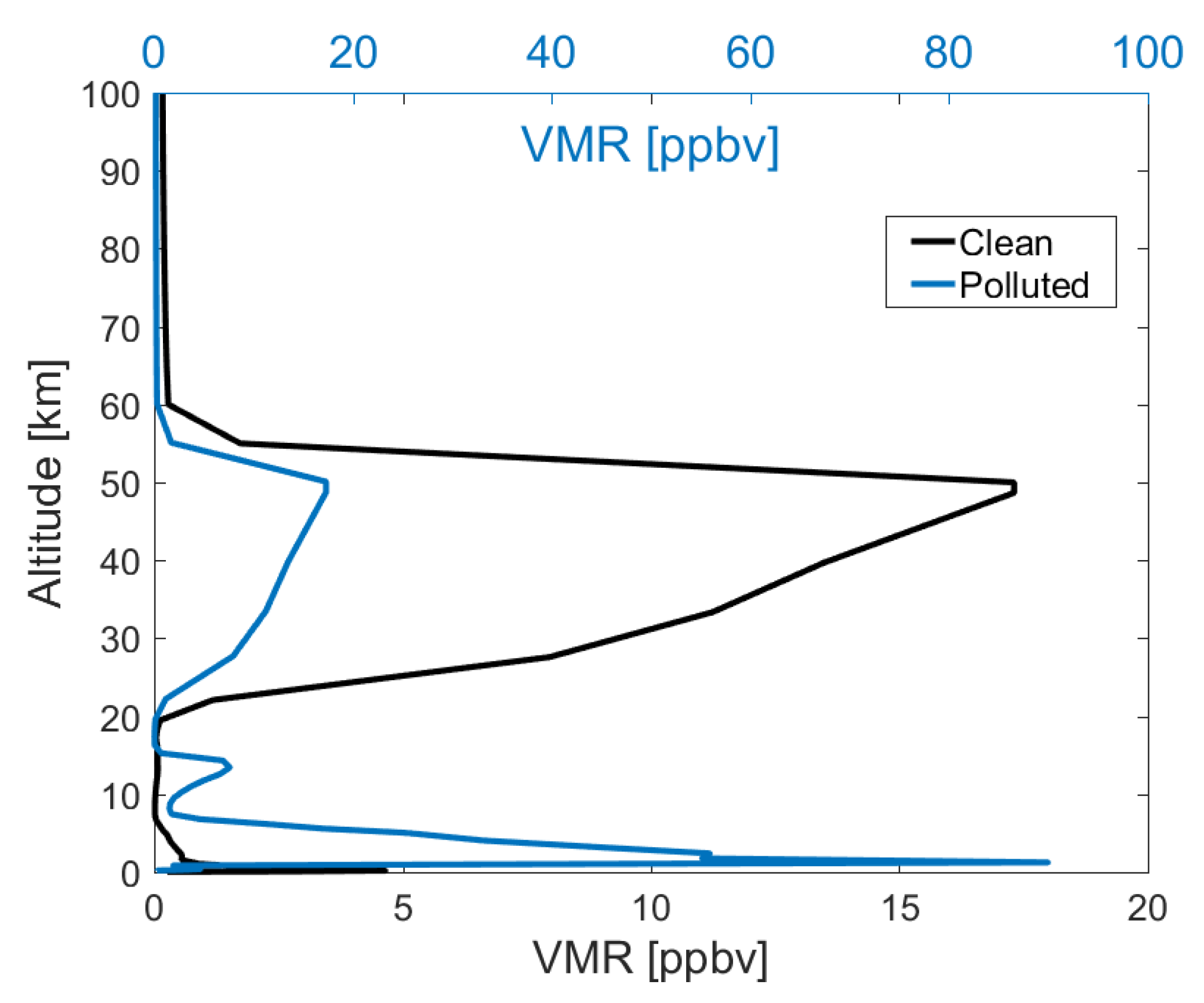
In this section, we analyze the numerical accuracy of the proposed inversion models. The radiances and the Jacobian matrices are computed by a radiative transfer model based on the discrete ordinate method with matrix exponential [45,46]. The spectral range is between 425 and 497 nm, the number of spectral points is $N_{\lambda }=345$, and the average spectral resolution is $\Delta {\lambda }_0=0.2$ nm. The calculations are performed for a mid-latitude summer atmosphere [47] with a solar zenith angle of $30°$, a relative azimuth angle of $180°$, and a Lambertian surface with albedo of $0.05$. The atmosphere between 0 and 50 km is discretized with a step of 0.5 km between 0 and 2 km, 1 km between 2 and 20 km, 5 km between 20 and 30 km, and 10 km between 30 and 50 km. The troposphere extends to an altitude of 15 km.

The simulations include the absorption of ${\mathrm{NO}}_2$, ozone (${\mathrm{O}}_3$), oxygen dimer (${\mathrm{O}}_4$), and water vapor, the Ring correction spectrum $S_1({\lambda }_k)=S_{\mathrm{R}}({\lambda }_k)$, the offset correction spectrum $S_2({\lambda }_k)=S_{\mathrm{O}}({\lambda }_k)$, and the wavelength shift $\Delta \lambda$. The scattering by clouds and aerosols is not taken into account. Vertical ${\mathrm{NO}}_2$ volume mixing ratio profiles for a clean scenario, which typically shows a larger concentration at higher altitudes, and a polluted scenario, which typically shows a larger concentration near the surface, are illustrated in Figure 1. These profiles are taken as a priori partial column profiles and used to generate the true (exact) partial column profiles.

Denoting the a priori partial columns of gas g by $x_{\mathrm{a}g,j}$, $j=1,\dots ,N_{\mathrm{lay}}$ and choosing cubic smoothing polynomials ($N=4$) and the amplitudes of the correction spectra as $b_1=b_{\mathrm{a}\mathrm{R}}=5\times {10}^{-2}$ and $b_2=b_{\mathrm{a}\mathrm{O}}={10}^{-2}$, we generate synthetic measurement spectra as follows:

• we choose $x_{g,j}^{†}=s_g{x}_{\mathrm{a}g,j}$ with $j=1,\dots ,N_{\mathrm{lay}}$ and $s_g=1.5$ (if not stated otherwise) and compute $X_g^{†}={\sum }_{j=1}^{N_{\mathrm{lay}}}{x}_{g,j}^{†}=s_g{X}_{\mathrm{a}g}$, $X_{\mathrm{s}{\mathrm{NO}}_2}^{†}={\sum }_{j=1}^{N_{\mathrm{t}}-1}{x}_{{\mathrm{NO}}_2,j}^{†}$ and $X_{\mathrm{t}{\mathrm{NO}}_2}^{†}={\sum }_{j=N_{\mathrm{t}}}^{N_{\mathrm{lay}}}{x}_{{\mathrm{NO}}_2,j}^{†}$; thus, the exact total ${\mathrm{NO}}_2$ column to be retrieved is $X_{{\mathrm{NO}}_2}^{†}=1.5X_{\mathrm{a}{\mathrm{NO}}_2}$;
• for ${\mathbf{X}}^{†}=[X_{{\mathrm{NO}}_2}^{†},X_{{\mathrm{O}}_3}^{†},X_{{\mathrm{O}}_4}^{†},X_{{\mathrm{H}}_2\mathrm{O}}^{†}]$, we compute $I_{\mathrm{sim}}({\lambda }_k,{\mathbf{X}}^{†})$ by the radiative transfer model;
• we determine the coefficients ${\mathbf{c}}_{\mathrm{sim}}({\mathbf{X}}^{†})$ of the smoothing polynomial $P_{\mathrm{sim}}({\lambda }_k,{\mathbf{c}}_{\mathrm{sim}}({\mathbf{X}}^{†}))$ by solving the least-squares problem (25);
• we compute $I_{\mathrm{sim}}^{\delta }({\lambda }_k,{\mathbf{X}}^{†})=I_{\mathrm{sim}}({\lambda }_k,{\mathbf{X}}^{†})+{\delta }_k$, where ${\delta }_k$ are independent Gaussian random variables with zero mean and standard deviation

  $${\sigma }_k=\frac{I_{\mathrm{sim}}({\lambda }_k,{\mathbf{X}}^{†})}{\mathrm{SNR}},$$

  and SNR is the signal-to-noise ratio;
• we choose $b_1^{†}=b_{\mathrm{R}}^{†}=2b_{\mathrm{a}\mathrm{R}}$, $b_2^{†}=b_{\mathrm{O}}^{†}=2b_{\mathrm{a}\mathrm{O}}$, and $▵{\lambda }^{†}=0.2\Delta {\lambda }_0$;
• for DRMI, we compute the kth component of the noisy data vector as

  $$R_{\mathrm{mes}}^{\delta }({\lambda }_k)=[ln{I}_{\mathrm{sim}}^{\delta }({\lambda }_k+▵{\lambda }^{†},{\mathbf{X}}^{†})-P_{\mathrm{sim}}({\lambda }_k,{\mathbf{c}}_{\mathrm{sim}}({\mathbf{X}}^{†}))]+\sum _{j=1}^{N_{\mathrm{s}}}{b}_j^{†}{S}_j({\lambda }_k);$$
• for DRME, we choose ${\mathbf{c}}^{†}=0.5{\mathbf{c}}_{\mathrm{sim}}({\mathbf{X}}^{†})$ and compute the kth component of the noisy data vector as

  $$R_{\mathrm{mes}}^{\delta }({\lambda }_k)=ln{I}_{\mathrm{sim}}^{\delta }({\lambda }_k+▵{\lambda }^{†},{\mathbf{X}}^{†})+\sum _{j=1}^{N_{\mathrm{s}}}{b}_j^{†}{S}_j({\lambda }_k)-P({\lambda }_k,{\mathbf{c}}^{†}).$$

Note that in view of the approximation

$$\begin{array}{cc}\hfill & ln{I}_{\mathrm{sim}}^{\delta }({\lambda }_k,{\mathbf{X}}^{†})\hfill \\ \hfill & \approx ln{I}_{\mathrm{sim}}({\lambda }_k,{\mathbf{X}}^{†})+\frac{{\delta }_k}{I_{\mathrm{sim}}({\lambda }_k,{\mathbf{X}}^{†})},\hfill \end{array}$$

the error in $ln{I}_{\mathrm{sim}}^{\delta }({\lambda }_k,{\mathbf{X}}^{†})$ is ${\delta }_{lnk}={\delta }_k/I_{\mathrm{sim}}({\lambda }_k,{\mathbf{X}}^{†})$, implying ${\sigma }_{lnk}=1/\mathrm{SNR}$ for all k. Thus, the error vector ${\delta }_{ln}$ is white noise with covariance matrix ${\sigma }_{lnk}^2{\mathbf{I}}_m$, where ${\mathbf{I}}_m$ is the identity matrix.

Some parameters characterizing the regularization algorithms are chosen as follows.

• As usual, the initial guess is taken to be equal to the a priori, i.e., ${\mathbf{x}}_0={\mathbf{x}}_{\mathrm{a}}$.
• If not stated otherwise, the regularization parameter of the method of Tikhonov regularization is chosen as $\alpha ={\sigma }_{lnk}^2$, while for the iteratively regularized Gauss–Newton method, the initial value of the regularization parameter is ${\alpha }_0={\sigma }_{lnk}$ and the regularization strength is gradually decreased during the iterative process with a constant ratio $q=0.2$. Because the iteratively regularized Gauss–Newton method is less sensitive to the overestimation of the regularization parameter, the choice of ${\alpha }_0\gg \alpha$ should guarantee that the method is able to capture the optimal value of the regularization parameter, i.e., ${\alpha }_{k^{\star }}\approx {\alpha }_{\mathrm{opt}}$.
• The weighting factors of the state vector in (26) and (27) are given by standard deviations for ${\left\{w_g\right\}}_{g=1}^{N_{\mathrm{g}}}$ and empirical values for ${\left\{w_{\mathrm{b}j}\right\}}_{j=1}^{N_{\mathrm{s}}}$ and ${\left\{w_{\mathrm{c}p}\right\}}_{p=1}^N$.
• The control parameter in the discrepancy principle Equation (15) is $\tau =1.2$.

Figure 2 shows the radiances $ln{I}_{\mathrm{sim}}(\lambda ,{\mathbf{X}}_{\mathrm{a}})$ and the differential radiances $ln{I}_{\mathrm{sim}}(\lambda ,{\mathbf{X}}_{\mathrm{a}})-P_{\mathrm{sim}}({\lambda }_k,{\mathbf{c}}_{\mathrm{sim}}({\mathbf{X}}_{\mathrm{a}}))$ for the clean and polluted ${\mathrm{NO}}_2$ profiles. For optically thin absorbers in the visible wavelength range, such as the clean ${\mathrm{NO}}_2$ profile, the absorption effect on the overall radiances is small. In contrast, for the polluted ${\mathrm{NO}}_2$ profile, the absorption is largely enhanced; the radiances decrease by more than 15% and show a spectral structure linked to the ${\mathrm{NO}}_2$ absorption bands. Due to the lack of a differential structure, we expect that the inversion models based on the analysis of differential spectra will have difficulties in handling the clean scenario, and in particular when the signal-to-noise ratio is small.

6.1. Total ${NO}_2$ Column Retrieval

In Figure 3, we illustrate the relative errors in the total ${\mathrm{NO}}_2$ column versus the signal-to-noise ratio for the clean scenario. The results correspond to DRMI and DRME and the two regularization methods (Tikhonov regularization and the iteratively regularized Gauss–Newton method). The following conclusions can be drawn.

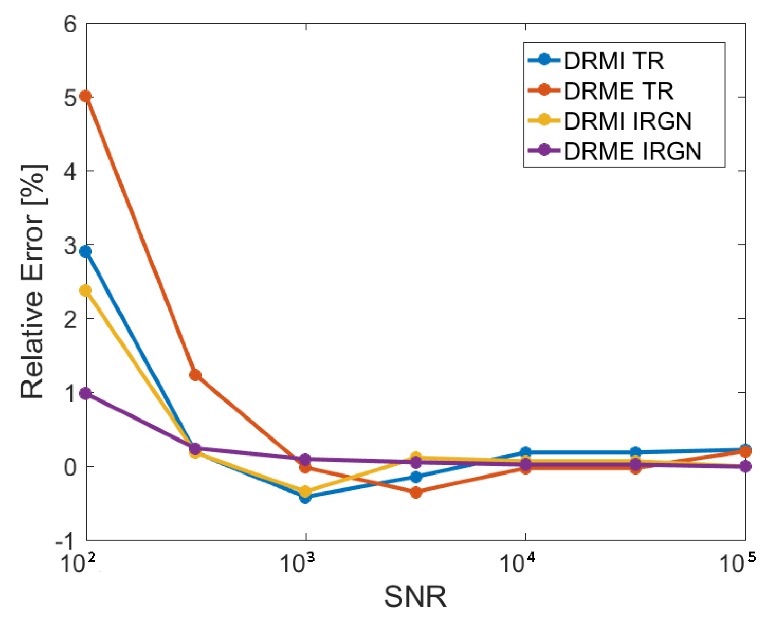
• The relative errors decrease with the increasing signal-to-noise ratio.
• In general, for small values of the signal-to-noise ratio ($\mathrm{SNR}<{10}^3$), the relative errors obtained by the iteratively regularized Gauss–Newton method are smaller than those delivered by the method of Tikhonov regularization. Note that for the clean scenario with $\mathrm{SNR}<{10}^3$ (where the ${\mathrm{NO}}_2$ signal is very low and the noise level is relatively high), the retrieval error is dominated by the noise error rather than the smoothing error.
• For small values of the signal-to-noise ratio ($\mathrm{SNR}<{10}^3$), DRMI equipped with the method of Tikhonov regularization delivers more reliable results than DRME; when the iteratively regularized Gauss–Newton method is used as regularization method, the reverse situation occurs.
• For large values of the signal-to-noise ratio ($\mathrm{SNR}\ge {10}^3$), the relative errors are within $\pm 0.5\%$ for all inversion models and regularization methods.

Figure 4 shows the variation of the square residuals, corresponding to DRMI and DRME in combination with the iteratively regularized Gauss–Newton method, versus the iteration step for the clean scenario. In Figure 4b, the variation of the regularization parameter ${\alpha }_k$ in the case of $\mathrm{SNR}={10}^3$ is also shown. The results demonstrate the basic features of the iterative regularization method.

• The residuals attain a plateau, which is used for estimating the noise level. This plateau is more pronounced for small values of the signal-to-noise ratio and decreases when the signal-to-noise ratio increases.
• At the initial guess, the residual corresponding to the DRMI model is much smaller than that corresponding to the DRME. The reason is that the discrepancies between the differential spectra are usually small. However, at the end of the iterative processes, the residuals are comparable.
• In DRMI, the residual decreases very fast at the first iteration step, while in DRME, there is a period of stagnation after which the residual decreases very rapidly.
• For small values of the signal-to-noise ratio ($\mathrm{SNR}\le {10}^3$), the iterative process in DRMI terminates after 3–4 iterations, while 10 iteration steps are required in DRME. However, the final residual in DRMI is slightly larger than in DRME; this result explains the larger relative errors provided by DRMI.
• In DRME and for $\mathrm{SNR}={10}^3$, the initial value of the regularization parameter is ${\alpha }_0={10}^{-3}$, while the final value, which is an estimate of the optimal value, is approximately equal to ${10}^{-6}$. Thus, the amount of regularization is small, and the solution coincides practically with the ordinary least-squares solution.

In Figure 5, we plot the absolute errors in the total ${\mathrm{NO}}_2$ column for the polluted scenario. The results correspond to DRME and the signal-to-noise ratio $\mathrm{SNR}={10}^3$. In this case, the regularization parameter of Tikhonov regularization corresponds to the optimal value predicted by the iteratively regularized Gauss–Newton method. The following observations can be noticed.

• The errors, obtained after one iteration step by the method of Tikhonov regularization, are large, and in particular when (i) the discrepancies between the values of the true and initial (a priori) total columns are significant, and (ii) the true values are lower than the initial values. However, the errors decrease significantly at the second iteration step, when they become comparable with the errors obtained by the iteratively regularized Gauss–Newton method. Recalling that the standard DOAS model is equivalent with the first iteration step of the DRME model (see Section 5), we conclude that the DOAS model can be used when the problem is not too nonlinear.
• An error up to $4\%$ is found for large values of the true total column, likely due to the stronger interference between the ${\mathrm{NO}}_2$ and Ring effect signatures [48] for polluted cases with deeper spectral structures (see Figure 2).

6.2. Tropospheric ${NO}_2$ Column Retrieval

Figure 6 shows the relative errors in the tropospheric ${\mathrm{NO}}_2$ column versus the signal-to-noise ratio for the clean scenario. The results are computed with (i) the nonlinear model, in which ${\mathbf{X}}_{-\overline{g}}=[X_{{\mathrm{O}}_3},X_{{\mathrm{O}}_4},X_{{\mathrm{H}}_2\mathrm{O}}]$ and $\mathbf{b}$ are determined in the pre-processing step by using DRMI and DRME, and (ii) the linear model, in which $X_{{\mathrm{NO}}_2}$ is again determined in the pre-processing step by means of DRMI and DRME. The regularization methods used in DRMI and DRME are the method of Tikhonov regularization and the iteratively regularized Gauss–Newton method. The following conclusions can be drawn.

• The relative errors of the linear model are smaller than those of the nonlinear model. This means that in the pre-processing step, the columns ${\mathbf{X}}_{-\overline{g}}$ of the auxiliary gases and the amplitudes $\mathbf{b}$ of the correction spectra are not accurately retrieved, while the total ${\mathrm{NO}}_2$ column $X_{{\mathrm{NO}}_2}$ is.
• For the linear model, the relative errors corresponding to the total column $X_{{\mathrm{NO}}_2}$ delivered by the iteratively regularized Gauss–Newton method are smaller than those delivered by the method of Tikhonov regularization. This result is not surprising because the first method yields more accurate total ${\mathrm{NO}}_2$ column retrievals than the second one (see Figure 3).
• The linear model using DRME in the pre-processing step in conjunction with the iteratively regularized Gauss–Newton method has the best retrieval performance; the relative errors are less than $5\%$ for $\mathrm{SNR}={10}^2$ and less than $2\%$ for $\mathrm{SNR}\ge {10}^3$.

The plots in Figure 7 illustrate the absolute errors in the tropospheric ${\mathrm{NO}}_2$ column for the polluted scenario. In the pre-processing step, only DRME is used to determine ${\mathbf{X}}_{-\overline{g}}=[X_{{\mathrm{O}}_3},X_{{\mathrm{O}}_4},X_{{\mathrm{H}}_2\mathrm{O}}]$ and $\mathbf{b}$ for the nonlinear model and $X_{{\mathrm{NO}}_2}$ for the linear model. The signal-to-noise ratio is $\mathrm{SNR}={10}^3$. The results lead to the following conclusions.

• In contrast to the clean scenario, the errors of the nonlinear model are smaller than those of the linear model. This means that the problem is nonlinear and that the linearizations (33) and (34) around the a priori do not describe the forward model accurately. Remember that the same conclusion has been drawn for the total ${\mathrm{NO}}_2$ column retrieval (see Figure 5).
• The corresponding errors of the nonlinear model are less than $0.3\%$, regardless of the regularization method used in the pre-processing step.

7. Conclusions

${\mathrm{NO}}_2$ columns retrieved from satellite remote sensing measurements have been successfully applied in many studies. The ${\mathrm{NO}}_2$ abundance is retrieved from the absorption structures of ${\mathrm{NO}}_2$ by analyzing the backscattered radiation in the visible spectral region. In this study, we have presented several inversion models for retrieving the total and tropospheric ${\mathrm{NO}}_2$ columns, which can be applied on spaceborne remote sensing data from current and upcoming hyperspectral instruments to characterize the spatial and temporal variation of ${\mathrm{NO}}_2$ concentrations.

For total column retrieval, we proposed the differential radiance models with internal and external closure, DRMI and DRME, respectively. The underlying nonlinear equations, involving, in addition to the total ${\mathrm{NO}}_2$ column, the total columns of the auxiliary gases, the amplitudes of the correction spectra, the coefficients of the smoothing polynomial, and the wavelength shift, are solved by means of regularization, that is, by using the method of Tikhonov regularization and the iteratively regularized Gauss–Newton method. Our numerical analysis showed that (i) for small values of the signal-to-noise ratio, DRMI along with the method of Tikhonov regularization yields more accurate results than DRME and that the reverse situation occurs when the iteratively regularized Gauss–Newton method is used as a regularization method, (ii) the iteratively regularized Gauss–Newton method is superior to the method of Tikhonov regularization because it is less sensitive to overestimations of the regularization parameter and can handle problems that actually do not require regularization, and finally, (iii) the best inversion model is DRME equipped with the iteratively regularized Gauss–Newton method.

The tropospheric column is retrieved in the framework of a nonlinear and a linear model by using (i) the results of the total column retrieval and (ii) the value of the stratospheric ${\mathrm{NO}}_2$ column delivered by a stratosphere–troposphere separation method. Specifically, in the nonlinear model, the nonlinear equations corresponding to DRMI or DRME are solved, while in the linear model, a linear equation that is the result of two linearity assumptions around the a priori is solved. Our numerical analysis revealed that for the clean scenario, when the problem is nearly linear, the linear model is superior to the nonlinear model, while for the polluted scenario, when the linearity assumption does not hold, the nonlinear model is better.

In our analysis, we also discussed the standard DOAS inversion model for total and tropospheric column retrieval and showed that this model is equivalent with the first iteration step of DRME for computing the total column and the linear model for computing the tropospheric column.

References

1. Solomon, S. Stratospheric ozone depletion: A review of concepts and history. Rev. Geophys. 1999, 37, 275–316. [Google Scholar] [CrossRef]
2. Seinfeld, J.; Pandis, S. Atmospheric Chemistry and Physics: From Air Pollution to Climate Change, 3rd ed.; Wiley: Hoboken, NJ, USA, 2016. [Google Scholar]
3. Shindell, D.T.; Faluvegi, G.; Koch, D.M.; Schmidt, G.A.; Unger, N.; Bauer, S.E. Improved attribution of climate forcing to emissions. Science 2009, 326, 716–718. [Google Scholar] [CrossRef] [PubMed]
4. Levelt, P.; Van den Oord, G.; Dobber, M.; Malkki, A.; Visser, H.; de Vries, J.; Stammes, P.; Lundell, J.; Saari, H. The Ozone Monitoring Instrument. IEEE Trans. Geosci. Remote Sens. 2006, 44, 1093–1101. [Google Scholar] [CrossRef]
5. Callies, J.; Corpaccioli, E.; Eisinger, M.; Hahne, A.; Lefebvre, A. GOME-2-Metop’s second-generation sensor for operational ozone monitoring. ESA Bull. 2000, 102, 28–36. [Google Scholar]
6. Munro, R.; Lang, R.; Klaes, D.; Poli, G.; Retscher, C.; Lindstrot, R.; Huckle, R.; Lacan, A.; Grzegorski, M.; Holdak, A.; et al. The GOME-2 instrument on the Metop series of satellites: Instrument design, calibration, and level 1 data processing—An overview. Atmos. Meas. Tech. 2016, 9, 1279–1301. [Google Scholar] [CrossRef]
7. Veefkind, J.; Aben, I.; McMullan, K.; Förster, H.; De Vries, J.; Otter, G.; Claas, J.; Eskes, H.; De Haan, J.; Kleipool, Q.; et al. TROPOMI on the ESA Sentinel-5 Precursor: A GMES mission for global observations of the atmospheric composition for climate, air quality and ozone layer applications. Remote Sens. Environ. 2012, 120, 70–83. [Google Scholar] [CrossRef]
8. Ingmann, P.; Veihelmann, B.; Langen, J.; Lamarre, D.; Stark, H.; Courrèges-Lacoste, G.B. Requirements for the GMES Atmosphere Service and ESA’s implementation concept: Sentinels-4/-5 and-5p. Remote Sens. Environ. 2012, 120, 58–69. [Google Scholar] [CrossRef]
9. Lambert, J.; Granville, J.; Allaart, M.; Blumenstock, T.; Coosemans, T.; De Maziere, M.; Friess, U.; Gil, M.; Goutail, F.; Ionov, D.; et al. Ground-Based Comparisons of Early SCIAMACHY O3 and NO2 Columns. In ESA Special Publication; European Space Agency: Paris, France, 2003; Volume 531. [Google Scholar]
10. Pinardi, G.; Van Roozendael, M.; Lambert, J.C.; Granville, J.; Hendrick, F.; Tack, F.; Yu, H.; Cede, A.; Kanaya, Y.; Irie, I.; et al. GOME-2 total and tropospheric NO2 validation based on zenith-sky, direct-sun and multi-axis DOAS network observations. In Proceedings of the 2014 EUMETSAT Meteorological Satellite Conference (EUMETSAT), Geneva, Swizerland, 22–26 September 2014. [Google Scholar]
11. Pinardi, G.; Lambert, J.C.; Granville, J.; Yu, H.; De Smedt, I.; van Roozendael, M.; Valks, P. O3M-SAF Validation Report; Technical Report, SAF/O3M/IASB/VR/NO2/TN-IASB-GOME2-O3MSAF-NO2-2015; EUMETSAT: Darmstadt, Germany, 2015. [Google Scholar]
12. Hilboll, A.; Richter, A.; Burrows, J. Long-term changes of tropospheric NO2 over megacities derived from multiple satellite instruments. Atmos. Chem. Phys. 2013, 13, 4145–4169. [Google Scholar] [CrossRef]
13. Hilboll, A.; Richter, A.; Burrows, J.P. NO2 pollution over India observed from space—The impact of rapid economic growth, and a recent decline. Atmos. Chem. Phys. Discuss. 2017. [Google Scholar] [CrossRef]
14. Zien, A.; Richter, A.; Hilboll, A.; Blechschmidt, A.M.; Burrows, J. Systematic analysis of tropospheric NO2 long-range transport events detected in GOME-2 satellite data. Atmos. Chem. Phys. 2014, 14, 7367–7396. [Google Scholar] [CrossRef]
15. Ding, J.; Miyazaki, K.; van der A, R.J.; Mijling, B.; Kurokawa, J.I.; Cho, S.; Janssens-Maenhout, G.; Zhang, Q.; Liu, F.; Levelt, P.F. Intercomparison of NOx emission inventories over East Asia. Atmos. Chem. Phys. 2017, 17, 10125. [Google Scholar] [CrossRef]
16. Visser, A.J.; Boersma, K.F.; Ganzeveld, L.N.; Krol, M.C. European NOx emissions in WRF-Chem derived from OMI: Impacts on summertime surface ozone. Atmos. Chem. Phys. 2019, 19, 11821–11841. [Google Scholar] [CrossRef]
17. Safieddine, S.; Clerbaux, C.; George, M.; Hadji-Lazaro, J.; Hurtmans, D.; Coheur, P.F.; Wespes, C.; Loyola, D.; Valks, P.; Hao, N. Tropospheric ozone and nitrogen dioxide measurements in urban and rural regions as seen by IASI and GOME-2. J. Geophys. Res. Atmos. 2013, 118. [Google Scholar] [CrossRef]
18. Varotsos, C.; Christodoulakis, J.; Tzanis, C.; Cracknell, A. Signature of tropospheric ozone and nitrogen dioxide from space: A case study for Athens, Greece. Atmos. Environ. 2014, 89, 721–730. [Google Scholar] [CrossRef]
19. Platt, U.; Stutz, J. Differential Optical Absorption Spectroscopy; Springer: Berlin/Heidelberg, Germany, 2008. [Google Scholar]
20. Burrows, J.P.; Weber, M.; Buchwitz, M.; Rozanov, V.; Ladstätter-Weißenmayer, A.; Richter, A.; DeBeek, R.; Hoogen, R.; Bramstedt, K.; Eichmann, K.U.; et al. The global ozone monitoring experiment (GOME): Mission concept and first scientific results. J. Atmos. Sci. 1999, 56, 151–175. [Google Scholar] [CrossRef]
21. Richter, A.; Burrows, J.P.; Nüß, H.; Granier, C.; Niemeier, U. Increase in tropospheric nitrogen dioxide over China observed from space. Nature 2005, 437, 129. [Google Scholar] [CrossRef]
22. Valks, P.; Pinardi, G.; Richter, A.; Lambert, J.C.; Hao, N.; Loyola, D.; Van Roozendael, M.; Emmadi, S. Operational total and tropospheric NO2 column retrieval for GOME-2. Atmos. Meas. Tech. 2011, 4, 1491. [Google Scholar] [CrossRef]
23. Van Geffen, J.; Boersma, K.; Van Roozendael, M.; Hendrick, F.; Mahieu, E.; De Smedt, I.; Sneep, M.; Veefkind, J. Improved spectral fitting of nitrogen dioxide from OMI in the 405–465 nm window. Atmos. Meas. Tech. 2015, 8, 1685–1699. [Google Scholar] [CrossRef]
24. Van Geffen, J.; Boersma, K.; Eskes, H.; Maasakkers, J.; Veefkind, J. TROPOMI ATBD of the Total and Tropospheric NO2 Data Products; Technical Report, S5P-KNMI-L2-0005-RP issue 1.4.0; KNMI: De Bilt, The Netherlands, 2019. [Google Scholar]
25. Liu, S.; Valks, P.; Pinardi, G.; De Smedt, I.; Yu, H.; Beirle, S.; Richter, A. An Improved Total and Tropospheric NO2 Column Retrieval for GOME-2. Atmos. Meas. Tech. 2019, 12, 1029–1057. [Google Scholar] [CrossRef]
26. Doicu, A.; Trautmann, T.; Schreier, F. Numerical Regularization for Atmospheric Inverse Problems; Springer Science & Business Media: Berlin/Heidelberg, Germany, 2010. [Google Scholar]
27. Tikhonov, A.N. On the solution of ill-posed problems and the method of regularization. Dokl. Akad. Nauk SSSR 1963, 151, 501–504. [Google Scholar]
28. Dennis, J.E., Jr.; Schnabel, R.B. Numerical Methods for Unconstrained Optimization and Nonlinear Equations; Society for Industrial and Applied Mathematics (SIAM): Philadelphia, PA, USA, 1996; Volume 16. [Google Scholar]
29. Gill, P.E.; Murray, W.; Wright, M.H. Practical Optimization; Academic Press: Cambridge, MA, USA, 1981. [Google Scholar]
30. Rodgers, C.D. Inverse Methods for Aatmospheric Sounding: Theory and Practice; World Scientific: Singapore, 2000; Volume 2. [Google Scholar]
31. Carissimo, A.; De Feis, I.; Serio, C. The physical retrieval methodology for IASI: The δ-IASI code. Environ. Model. Softw. 2005, 20, 1111–1126. [Google Scholar] [CrossRef]
32. Xu, J.; Schreier, F.; Doicu, A.; Trautmann, T. Assessment of Tikhonov-type regularization methods for solving atmospheric inverse problems. J. Quant. Spectrosc. Radiat. Transf. 2016, 184, 274–286. [Google Scholar] [CrossRef] [Green Version]
33. Wahba, G. Practical approximate solutions to linear operator equations when the data are noisy. SIAM J. Numer. Anal. 1977, 14, 651–667. [Google Scholar] [CrossRef]
34. Hansen, P.C. Analysis of discrete ill-posed problems by means of the L-curve. SIAM Rev. 1992, 34, 561–580. [Google Scholar] [CrossRef]
35. Bakushinskii, A.B. The problem of the convergence of the iteratively regularized Gauss–Newton method. Zhurnal Vychislitel’noi Mat. Mat. Fiz. 1992, 32, 1503–1509. [Google Scholar]
36. Morozov, V.A. On the solution of functional equations by the method of regularization. Dokl. Akad. Nauk SSSR 1966, 167, 510–512. [Google Scholar]
37. Huijnen, V.; Eskes, H.J.; Poupkou, A.; Elbern, H.; Boersma, K.F.; Foret, G.; Sofiev, M.; Valdebenito, A.; Flemming, J.; Stein, O.; et al. Comparison of OMI NO2 tropospheric columns with an ensemble of global and European regional air quality models. Atmos. Chem. Phys. 2010, 10, 3273–3296. [Google Scholar] [CrossRef]
38. Richter, A.; Burrows, J. Tropospheric NO2 from GOME measurements. Adv. Space Res. 2002, 29, 1673–1683. [Google Scholar] [CrossRef]
39. Bucsela, E.; Krotkov, N.; Celarier, E.; Lamsal, L.; Swartz, W.; Bhartia, P.; Boersma, K.; Veefkind, J.; Gleason, J.; Pickering, K. A new stratospheric and tropospheric NO2 retrieval algorithm for nadir-viewing satellite instruments: Applications to OMI. Atmos. Meas. Tech. 2013, 6, 2607. [Google Scholar] [CrossRef]
40. Beirle, S.; Hörmann, C.; Jöckel, P.; Liu, S.; Penning de Vries, M.; Pozzer, A.; Sihler, H.; Valks, P.; Wagner, T. The STRatospheric Estimation Algorithm from Mainz (STREAM): Estimating stratospheric NO2 from nadir-viewing satellites by weighted convolution. Atmos. Meas. Tech. 2016, 9, 2753–2779. [Google Scholar] [CrossRef]
41. Eskes, H.; Van Velthoven, P.; Valks, P.; Kelder, H. Assimilation of GOME total-ozone satellite observations in a three-dimensional tracer-transport model. Q. J. R. Meteorol. Soc. 2003, 129, 1663–1681. [Google Scholar] [CrossRef]
42. Dirksen, R.J.; Boersma, K.F.; Eskes, H.J.; Ionov, D.V.; Bucsela, E.J.; Levelt, P.F.; Kelder, H.M. Evaluation of stratospheric NO2 retrieved from the Ozone Monitoring Instrument: Intercomparison, diurnal cycle, and trending. J. Geophys. Res. Atmos. 2011, 116, D08305. [Google Scholar] [CrossRef]
43. Bucsela, E.J.; Celarier, E.A.; Wenig, M.O.; Gleason, J.F.; Veefkind, J.P.; Boersma, K.F.; Brinksma, E.J. Algorithm for NO2 vertical column retrieval from the ozone monitoring instrument. IEEE Trans. Geosci. Remote Sens. 2006, 44, 1245–1258. [Google Scholar] [CrossRef]
44. Rozanov, A.; Rozanov, V.; Buchwitz, M.; Kokhanovsky, A.; Burrows, J. SCIATRAN 2.0—A new radiative transfer model for geophysical applications in the 175–2400 nm spectral region. Adv. Space Res. 2005, 36, 1015–1019. [Google Scholar] [CrossRef]
45. Doicu, A.; Trautmann, T. Discrete-ordinate method with matrix exponential for a pseudo-spherical atmosphere: Scalar case. J. Quant. Spectrosc. Radiat. Transf. 2009, 110, 146–158. [Google Scholar] [CrossRef]
46. Doicu, A.; Trautmann, T. Discrete-ordinate method with matrix exponential for a pseudo-spherical atmosphere: Vector case. J. Quant. Spectrosc. Radiat. Transf. 2009, 110, 159–172. [Google Scholar] [CrossRef]
47. Anderson, G.P.; Clough, S.A.; Kneizys, F.; Chetwynd, J.H.; Shettle, E.P. AFGL Atmospheric Constituent Profiles (0.120 km); Technical Report; Air Force Geophysics Lab.: Hanscom AFB, MA, USA, 1986. [Google Scholar]
48. Marchenko, S.; Krotkov, N.; Lamsal, L.; Celarier, E.; Swartz, W.; Bucsela, E. Revising the slant column density retrieval of nitrogen dioxide observed by the Ozone Monitoring Instrument. J. Geophys. Res. Atmos. 2015, 120, 5670–5692. [Google Scholar] [CrossRef] [Green Version]
Figure 1. Vertical NO 2 volume mixing ratio (VMR) profiles for the clean and polluted scenarios. Note that both profiles have the same stratospheric NO 2 column.
Atmosphere 10 00607 g001
Figure 2. (a) Radiances and (b) differential radiances for the clean and polluted scenarios.
Atmosphere 10 00607 g002
Figure 3. Relative errors in the total NO 2 column as a function of signal-to-noise ratio (SNR). The results correspond to the clean scenario and are computed by means of the differential radiance model with internal closure (DRMI) and differential radiance model with external closure (DRME) models using the method of Tikhonov regularization (TR) and the iteratively regularized Gauss–Newton (IRGN) method.
Atmosphere 10 00607 g003
Figure 4. Square residuals computed by means of the (a) DRMI and (b) DRME models as a function of iteration number. The iteratively regularized Gauss–Newton (IRGN) method is applied, and the results correspond to the clean scenario. The iteration steps with the estimated optimal regularization parameter are marked (circles). For DRME and SNR = 10 3 , the history of the regularization parameter is also shown (green line).
Atmosphere 10 00607 g004
Figure 5. Absolute errors in the total NO 2 column for different values of the true total column. The results correspond to the polluted scenario and are computed by means of DRME using the method of Tikhonov regularization (TR) and the iteratively regularized Gauss–Newton (IRGN) method. The signal-to-noise ratio is SNR = 10 3 , and the vertical line shows the initial value of the total column.
Atmosphere 10 00607 g005
Figure 6. Relative errors in the tropospheric NO2 column as a function of SNR. The results are computed by means of linear and nonlinear models using in the pre-processing step the DRMI and DRME models in conjunction with (a) the method of Tikhonov regularization (TR) and (b) the iteratively regularized Gauss–Newton (IRGN) method.
Atmosphere 10 00607 g006
Figure 7. Absolute errors in the tropospheric NO 2 column for different values of the true tropospheric columns. The results correspond to the polluted scenario and are computed by means of linear and nonlinear models and using in the pre-processing step the DRME model in conjunction with Tikhonov regularization (TR) and the iteratively regularized Gauss–Newton (IRGN) method. The signal-to-noise ratio is SNR = 10 3 , and the vertical line shows the initial value of the tropospheric column.
Atmosphere 10 00607 g007