Article

Evaluation of Surface Radiative Fluxes over the Tropical Oceans in AMIP Simulations

1
Meteorology, Florida Institute of Technology, Melbourne, FL 32901, USA
2
US Naval Academy, Annapolis, MD 21402, USA
3
International Laboratory on Climate and Environment Change and Key Laboratory of Meteorological Disaster of Ministry of Education, Nanjing University of Information Science and Technology, Nanjing 210044, China
*
Author to whom correspondence should be addressed.
Atmosphere 2019, 10(10), 606; https://doi.org/10.3390/atmos10100606
Submission received: 23 September 2019 / Revised: 4 October 2019 / Accepted: 5 October 2019 / Published: 9 October 2019
(This article belongs to the Section Meteorology)

Abstract

:
The performance of 20 models from the Atmospheric Model Intercomparison Project (AMIP) was evaluated concerning surface radiation over the tropical oceans (30° S–30° N) from 1979 to 2000. The model ensemble mean of the net surface shortwave radiation (QSW) was underestimated compared to the International Satellite Cloud Climatology Project (ISCCP) data by 4 W m−2. On the other hand, net longwave radiation (QLW) was overestimated by 4 W m−2, leading to an underestimation of the net surface radiation (Qrad) by 8 W m−2. The most prominent bias in the Qrad appears to be over regions of low-level clouds in the off-equatorial eastern Pacific, eastern Atlantic, and the south-eastern Indian Ocean. The root means squared error of QLW was larger than that of QSW in 17 out of 20 AMIP models. Overestimation of the total cloud cover and atmospheric humidity contributed to the underestimation of Qrad. In general, models with higher horizontal resolutions performed slightly better than those with coarser horizontal resolutions, although some systematic bias persists in all models and in all seasons, in particular, in regions of low-level clouds for QLW, and high-level clouds for QSW. The ensemble mean performed better than most models, but two high-resolution models (GFDL-HIRAM-C180 and GFDL-HIRAM-C360) outperform the model ensemble.

1. Introduction

The spatio-temporal distribution of surface energy plays an essential role in determining the weather and climate on our planet (e.g., [1]). It has been recognized for a long time that the heat balance on the earth’s surface is as important as that at the top of the earth’s atmosphere for short-term weather fluctuations and long-term climate change [2]. As a result, it is important to evaluate the surface energy budget from global models. Kiehl and Trenberth [3] presented the global mean energy budget using satellite data and gridded reanalysis products. They found that factors like atmospheric water vapor, greenhouse gases, and clouds can greatly affect the radiation budget, and concluded that improved measurements are needed to lower the uncertainties in the annual global mean energy budget. Although the incoming and outgoing energy must balance globally, they do not balance locally or regionally [4]. Apart from the variation in the surface energy budget, there is also variation in the atmospheric heat budget [2].
A key component of the surface energy budget is the surface heat flux, which contributes to the exchange of mass and energy between the ocean and the atmosphere, and thereby, influences the oceanic and atmospheric circulations. The net surface heat flux (Qnet) includes latent heat QLH, sensible heat QSH, net longwave radiation QLW, and net shortwave radiation QSW. In this study, we provide an assessment of 20 atmospheric global climate models (AGCMs) participating in the Atmospheric Model Intercomparison Project (AMIP, [5]) in their ability to simulate surface radiation. We confine our assessment to the tropical oceans because they receive the most amount of solar radiation and play an important role in affecting the earth’s climate system due to their large heat capacity. We conduct our analysis over 30° S–30° N; the surface area of this latitudinal band is about 50% of the earth’s surface.
Surface radiative fluxes, QLW and QSW, can be split into upwelling and downwelling components. The net longwave (QLW) at the surface is given by:
Q L W =   Q U L W Q D L W ,
where QULW is the upward, and QDLW is the downward longwave radiation. The QULW is determined by the surface temperature (Ts) of the ocean according to the Stefan–Boltzmann law:
Q L W = ε σ T s 4 Q D L W ,
where ε is the surface emissivity, and σ is the Stefan–Boltzmann constant (5.67 × 10⁻⁸ W m−2 K−4).
Similarly, QSW at the surface is given by:
Q S W = Q D S W Q U S W ,
where QUSW is only a function of the surface albedo and QDSW. Therefore, Equation (3) could be written as:
Q S W = Q D S W × ( 1 α ) ,
where α is the surface albedo.
Many past studies have focused on downward shortwave radiation (QDSW) instead of downward longwave radiation (QDLW) because QDLW is not conventionally measured (e.g., [6,7]). Since the QDSW depends on the atmospheric constituents like water vapor and cloud, simulated QDSW is affected by the cloud parameterization in the model (e.g., [8]) and is one of the most important factors in the exchange of energy between earth’s surface and the atmosphere (e.g., [9]). Wild et al. [10] verified QDLW using direct observations gathered in the Global Energy Balance Archive [9,11]. Garratt and Prata [12] found that the QDLW is typically underestimated in global climate models (GCMs), and evidence suggests that bias persists for both all- and clear-sky conditions [9,13].
There are several unique aspects in our evaluation study of surface radiation: First, most of the earlier studies have used coupled models (e.g., [13,14]) for the evaluation of surface radiation. The number of studies related to atmospheric models is far fewer. Understanding the biases in surface radiation in atmospheric models may help to understand its coupled counterpart. In particular, prescribed sea surface temperature (SST) in AMIP simulations eliminates possible biases from errors in SST [15]. Second, we also use long-term surface radiation data from moored buoys over the tropical oceans. To the best of our knowledge, these data have not been used for a systematic evaluation of atmospheric models. Third, prior studies have not been undertaken to assess the seasonal variability of bias in AMIP simulated surface radiation.
In this study, we evaluate AMIP models concerning their ability to capture surface radiative fluxes compared to the satellite and in situ observations over the tropical oceans. The global models with coarse horizontal resolutions may not capture the convection and clouds over the tropical oceans. This is expected to lead to bias in the surface radiation that is influenced by the atmospheric as well as surface properties. However, no quantitative evaluation has been presented for AMIP models that show the geographical and seasonal distribution of the bias. The possible causes behind model bias and its dependence on horizontal resolutions are also explored.
The rest of the paper is organized as follows. Description of the models and data are given in Section 2. Model-data comparison is presented in Section 3, followed by an exploration of the causes behind the model bias in Section 4. The extent to which the model bias is dependent on the model horizontal resolutions is explored in Section 5. Summary and conclusions are given in Section 6.

2. Model, Data, and Method

We use the output from 20 AMIP models that are involved with the Coupled Model Intercomparison Project (CMIP, [16]) for this study (Table 1). The choice of these models was based upon the availability of all the parameters needed for this study. Specified boundary conditions were used for all AMIP models [5,17]. Therefore, the inter-model differences are due to the internal dynamics of the models and are not due to the surface boundary conditions. The reference for each model is also provided in Table 1.
For model validation, we used surface radiation from the International Satellite Cloud Climate Project (ISCCP, 1° × 1°, [18]) that is available from the Objectively Analyzed air-sea heat Fluxes (OAFlux, 1° × 1°, [19]) dataset. However, the net heat flux data in OAFlux is assimilated using the ISCCP and other datasets [19]. The ISCCP data have been extensively used to improve the understanding and modeling of the earth’s radiation (e.g., [20,21]). We also use ISCCP-D2 [21] for total cloud cover and precipitable water. The ISCCP-D2 uses observations in the visible and infrared window portion of the spectrum to determine total cloud amount as well as low-, mid-, and high-level clouds, and the total precipitable water (TPW) amount [18]. In addition to the ISCCP data, we analyzed observations of surface radiative fluxes from moored buoys (Figure 1) that include the Tropical Atmosphere Ocean (TAO) array (63 buoys) in the Pacific, the Prediction and Research Moored Array in the Tropical Atlantic (PIRATA) array (18 buoys) in the Atlantic, and the Research Moored Array for African-Asian-Australian Monsoon Analysis and Prediction (RAMA) array (10 buoys) in the Indian Ocean.
The annual mean shortwave and longwave radiation at the surface measured by the buoys have an uncertainty of about 5–6 W m−2, and 4 W m−2, respectively [39,40]. For the ISCCP, the biases in the monthly shortwave and longwave fluxes are less than 5 W m−2 [41] and 3 W m−2 [42], respectively, and are smaller for the annual means. For a consistent comparison, all the models and ISCCP data over 21 years (1979–2000) were bilinearly interpolated to monthly values in 2.5° × 2.5° boxes as the original ISCCP data is 3 hourly with 2.5° × 2.5° resolution. For comparison with buoys, we limit our calculation to 12 years (1997–2008) when all the buoy data are available. Note that, although ISCCP provides data for the total cloud cover, as well as low-, mid-, and high-level clouds [18], AMIP models only provide information for the total cloud cover. As a result, we only estimate bias in the total cloud cover for AMIP models. Also, monthly mean total cloud cover in AMIP includes both day and night, while QSW is influenced by cloud cover only during the daytime. As a result, the bias in QSW due to bias in cloudiness was not explored in this study.

3. Model-data Comparisons

In this section, we provide a detailed comparison of the QLW and QSW from AMIP simulations with those from the OAFlux dataset and moored buoys. In addition to the climatological mean, we also look at the seasonal cycle of the surface radiation over different ocean basins.

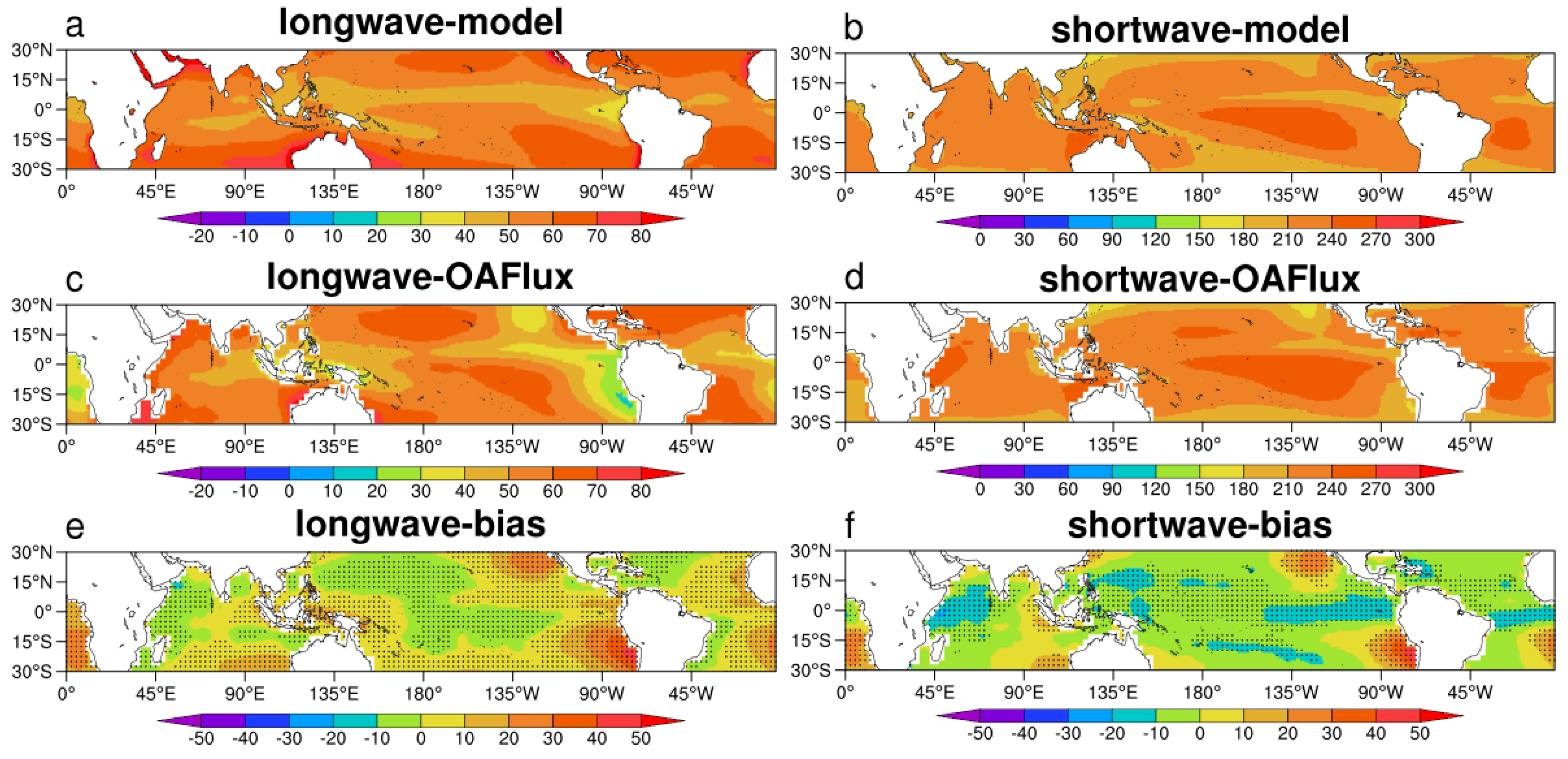
3.1. Comparison with OAFlux

The climatological mean of the model ensemble (Figure 2a,b) and OAFlux data (Figure 2c,d) show that the overall horizontal structure of surface radiation has been captured well. In particular, the bias in QLW (Figure 2e) near the equator is within 10 W m−2. The bias in QSW (Figure 2f) is also small (<10 W m−2) near the equator. The most prominent bias in radiation appears over the off-equatorial eastern Pacific and the eastern Atlantic where the bias is statistically significant at the 95% level using a Student’s t-test. There are, however, inter-model differences (Figure 3 and Figure 4). For QLW (Figure 3), even though most models show a large bias (~30 W m−2) in the off-equatorial eastern Pacific Ocean as seen in the model ensemble mean (Figure 2e), the magnitude of the bias varies in different models. Only two models (INM-CM4 and MIROC5 in Figure 3) show negative mean bias (i.e., underestimation of QLW) when averaged over the entire tropical oceans which is consistent with earlier studies (e.g., [12]). For QSW (Figure 4), about half of the models underestimate it. The overestimation of QSW in the off-equatorial Pacific (Figure 4) is seen in all models with varying magnitudes and is consistent with the bias in QSW in Figure 3. This indicates the possible role of clouds over cooler SST. All 20 models show higher correlation coefficient (CC) in QSW than QLW. Wild et al. [13], and all 20 models found a high correlation between models and observation for QSW. We believe this difference in the model skill concerning surface radiation exists because the QDLW is a complex variable to capture in any model and is not conventionally measured (e.g., [6]).
The latitudinal distribution of bias in QLW in the Indian Ocean (Figure 5a, red) shows a maximum bias around the equator that gradually reduces to a minimum around 15° N and 15° S latitudes before increasing again at higher latitudes. In the Pacific (Figure 5b, red), the minimum bias is around 15° N, similar to the Indian Ocean (Figure 5a). In the Atlantic (Figure 5c, red), QLW bias decreases gradually northward from around 15° S. Given that the models were forced by the observed SST, errors in QLW (see Equation (2)) come from the QDLW in the atmosphere and are explored in Section 4. The latitudinal variation in QSW bias shows underestimation (~8–14 W m−2) close to the equator (Figure 5, blue) in the presence of the Inter-tropical Convergence Zone (ITCZ), implying that the cloud cover in the model might have been overestimated in the models (see further in Section 4). Such bias remains a common problem even for higher resolution models (e.g., [43,44])
The seasonal variation of bias in QLW (Figure 6, left) shows that models overestimate QLW over the eastern Pacific and eastern Atlantic in all seasons. In the central pacific, away from the equator, QLW is underestimated during June-July-August (JJA, Figure 6e) and September-October-November (SON, Figure 6g). In the Arabian sea, QLW is underestimated in all seasons except during the summer monsoon months (Figure 6e). Therefore, the models have large regional and seasonal biases and do not often close the surface heat budget (e.g., [45]). For Qsw (Figure 6, right), the horizontal distribution of bias also shows some systematic patterns. For example, there is a negative bias in the northwestern Indian ocean in all seasons except during the JJA. There is positive bias in the eastern south Atlantic Ocean and in the off-equatorial eastern Pacific, which is consistent with Zhang et al. [46], who also found that models have a positive bias in QSW in the tropics. In the Atlantic, the hemispheric pattern of bias reverses from DJF (Figure 6b) to JJA (Figure 6f). The seasonal bias in surface radiation and net heat flux is summarized in Table 2. The possible reasons for such bias in surface radiative fluxes are discussed in Section 4.

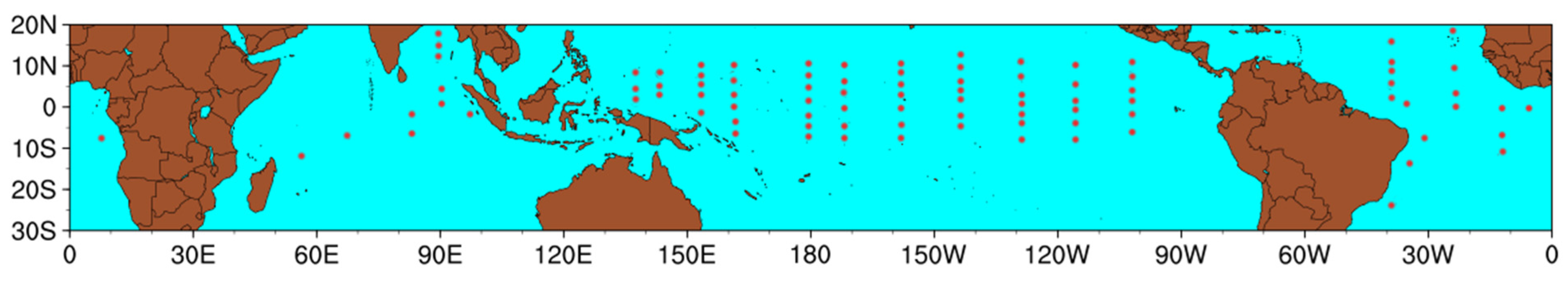
3.2. Comparison with Buoy Data

The surface radiation from the model and OAFlux are compared with moored buoys in Figure 7. The OAFlux generally agrees well with the moored buoys, which provides confidence in our use of OAFlux for model evaluation. The time-series of the model ensemble mean captures the seasonal variability but always underestimates QSW and overestimates QLW, implying again that there is systematic error in the model possibly coming from the overestimation of cloud and atmospheric water vapor. The seasonal and annual mean bias compared to the buoy data is shown in Table 2. In both QLW and QSW, the results are similar when compared to buoys and to OAFlux because radiation from buoys and OAFlux were similar (Figure 7). For bias in Qnet, QSW, and QLW have similar contributions; but the major contribution of bias in Qnet comes from the surface turbulent heat fluxes.

4. On the Causes Behind Model Bias
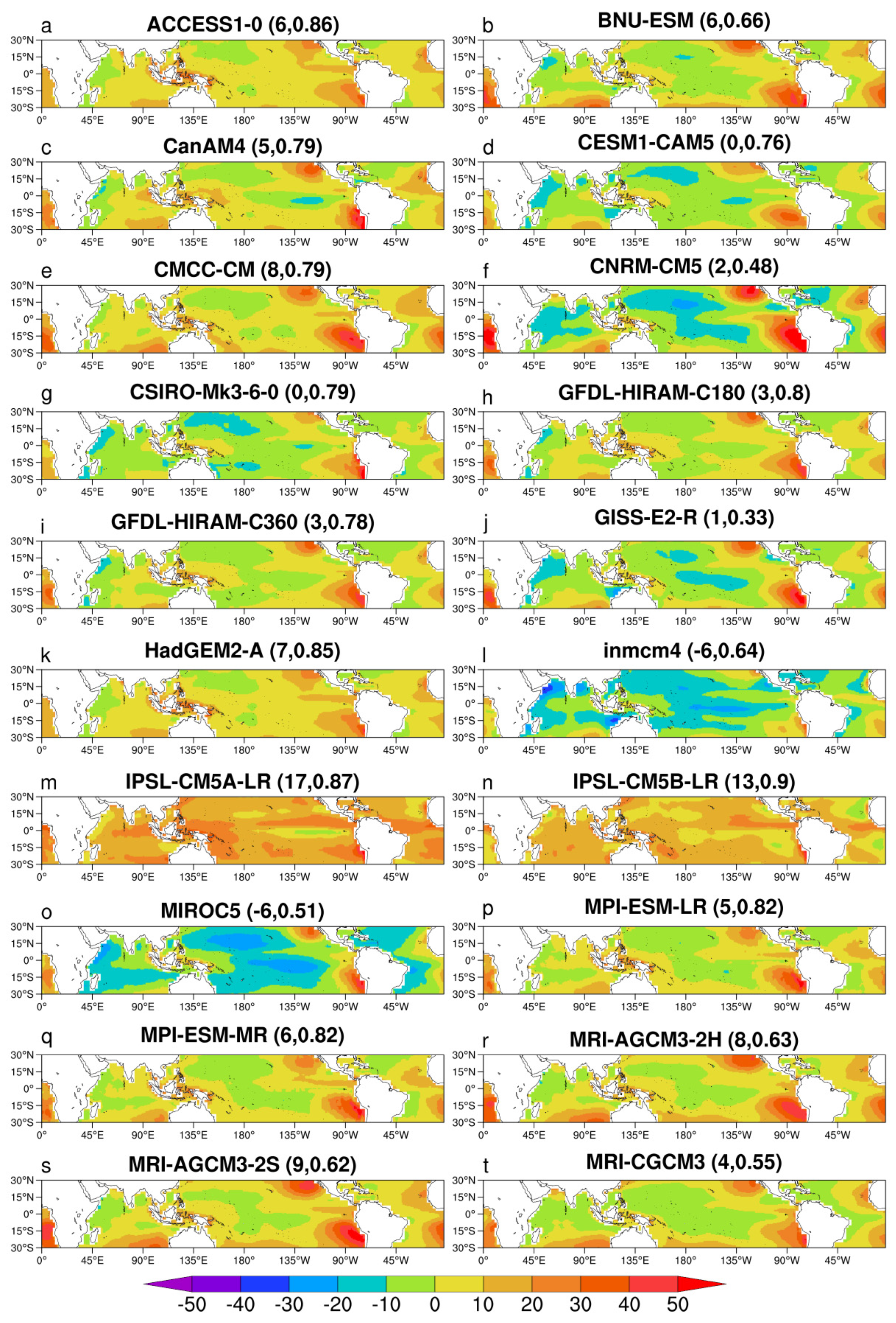
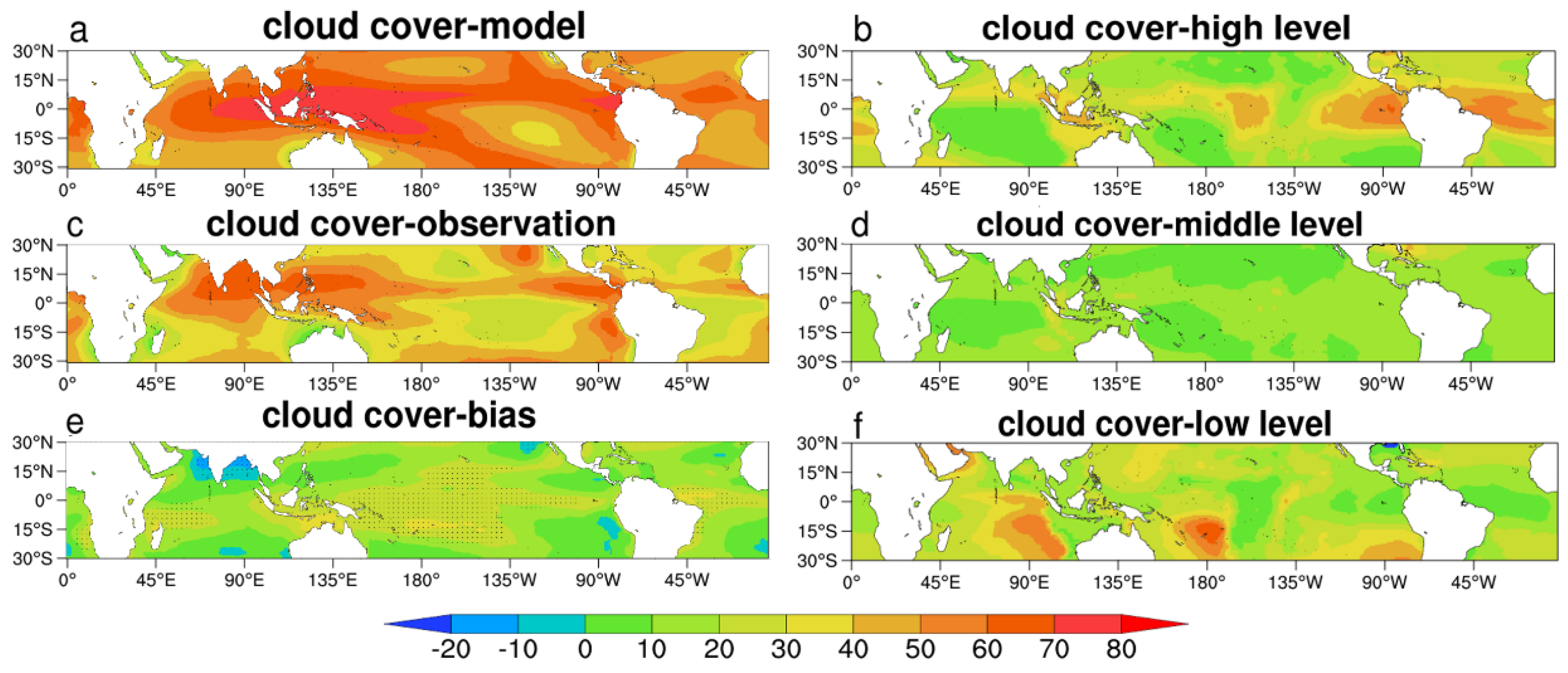
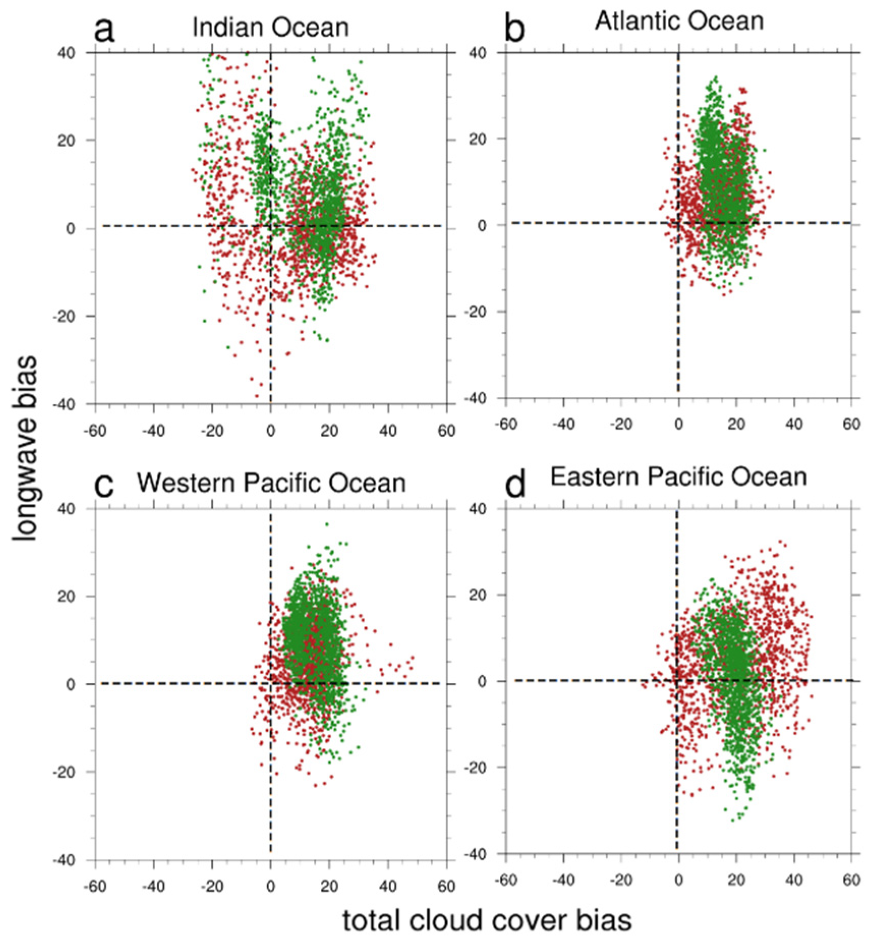
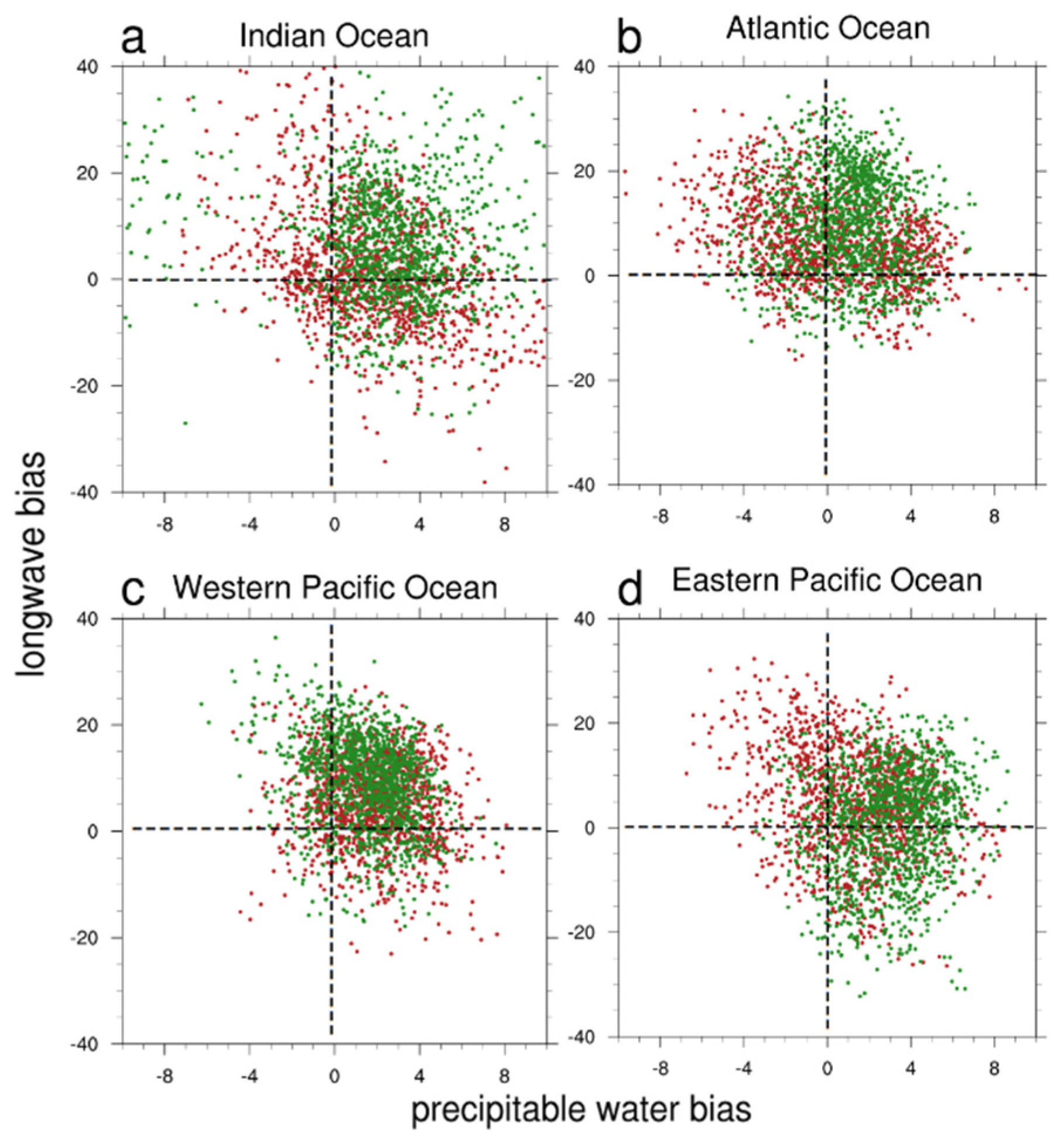
Models can have significant uncertainties because of inaccuracies in input data and in the surface flux retrieval algorithms or methods [47]. In this section, we explore the causes behind the commonalities and differences between the simulated and observed radiation, with an emphasis on the role played by different variables (e.g., cloud cover, atmospheric water vapor) that influence the surface radiation.

4.1. Longwave (QLW)

The evaluation of the spatial structure of the simulated QLW (Figure 8a) shows that the CC (correlation) is between 0.33 (GISS-E2-R) and 0.90 (IPSL-CM5B-LR). The standard deviation (SD, the ratio of model standard deviation and observed standard deviation) is from 0.60 (GISS-E2-R) to 1.10 (IPSL-CM5A-LR). The QLW bias is expected to come from bias in cloud cover and atmospheric water vapor content. The simulated cloud cover is better represented during the boreal summer (Figure 8c) than that in boreal winter (Figure 8b). This seasonal difference in cloud cover bias leads to a larger bias in surface radiation during JJA than DJF (Table 2). For example, compared to the buoy data, the bias in QLW and QSW during DJF is 1 and −4 W m−2 compared to those during JJA of 3 and −5 W m−2. Most of the bias in QLW comes from the QDLW (and not from the QULW) since QULW is determined by the SST, and the SST was provided from observations. Similarly, the bias in QSW comes from the QDSW, which is influenced by the cloud cover and atmospheric water vapor content. Models tend to underestimate TPW in DJF (Figure 8b) but overestimate it in JJA (Figure 8c). The correlation is higher in JJA than DJF for TPW.
The simulated total cloud cover is overestimated compared to the observation in most of the tropics except parts of the southeastern Indian Ocean and eastern Pacific (Figure 9). One should, however, be careful regarding the accuracy of the observed cloud cover. For example, high- (Figure 9b), mid- (Figure 9d) and low-level (Figure 9f) clouds in ISCCP are observed from the satellite level. Therefore, mid-level clouds are those that are not obstructed by high-level clouds [21,48]. Similarly, low-level clouds are those that are not blocked by high- and mid-level clouds. The locations of the low-level cloud cover (Figure 9f) are the regions mainly covered by stratus and stratocumulus clouds over cooler SST (e.g., [49,50]). In the absence of cloud cover information at high-, mid-, and low-levels from the AMIP simulations, we only show how the bias in QLW and QSW varies with the bias in total cloud cover. Huber et al. [51] also found that the radiative fluxes show a high correlation with the total cloud cover and the atmospheric water vapor.
The relationship between the bias in QLW and bias in total cloud cover and TPW from boreal winter (DJF) and summer (JJA) is presented in Figure 10 and Figure 11 over different tropical oceans. With an overestimation in cloud cover (Figure 10), QLW is generally overestimated, indicating that QDLW is underestimated (e.g., [12]). As expected, a positive bias in QLW appears when the cloud cover bias is also positive over the Atlantic (Figure 10b, top right quadrant), and Pacific (Figure 10c,d, top right quadrant), but this relationship is less clear over the Indian Ocean (Figure 10a), especially during DJF. For regions with around 20% bias in cloud cover, the QLW bias has a broad range. Such larger variation possibly comes from the height and other optical properties of the cloud and atmospheric water vapor content. Similar to the cloud cover, TPW is also overestimated in most parts of the tropical oceans (Figure 11). Irrespective of overestimation or underestimation in TPW, the QLW bias is mostly positive, a result that also suggests its dependence on cloud cover (Figure 10). Overall, during the JJA, the TPW bias is positive in all ocean basins, but during the DJF, TPW bias can be negative as well.

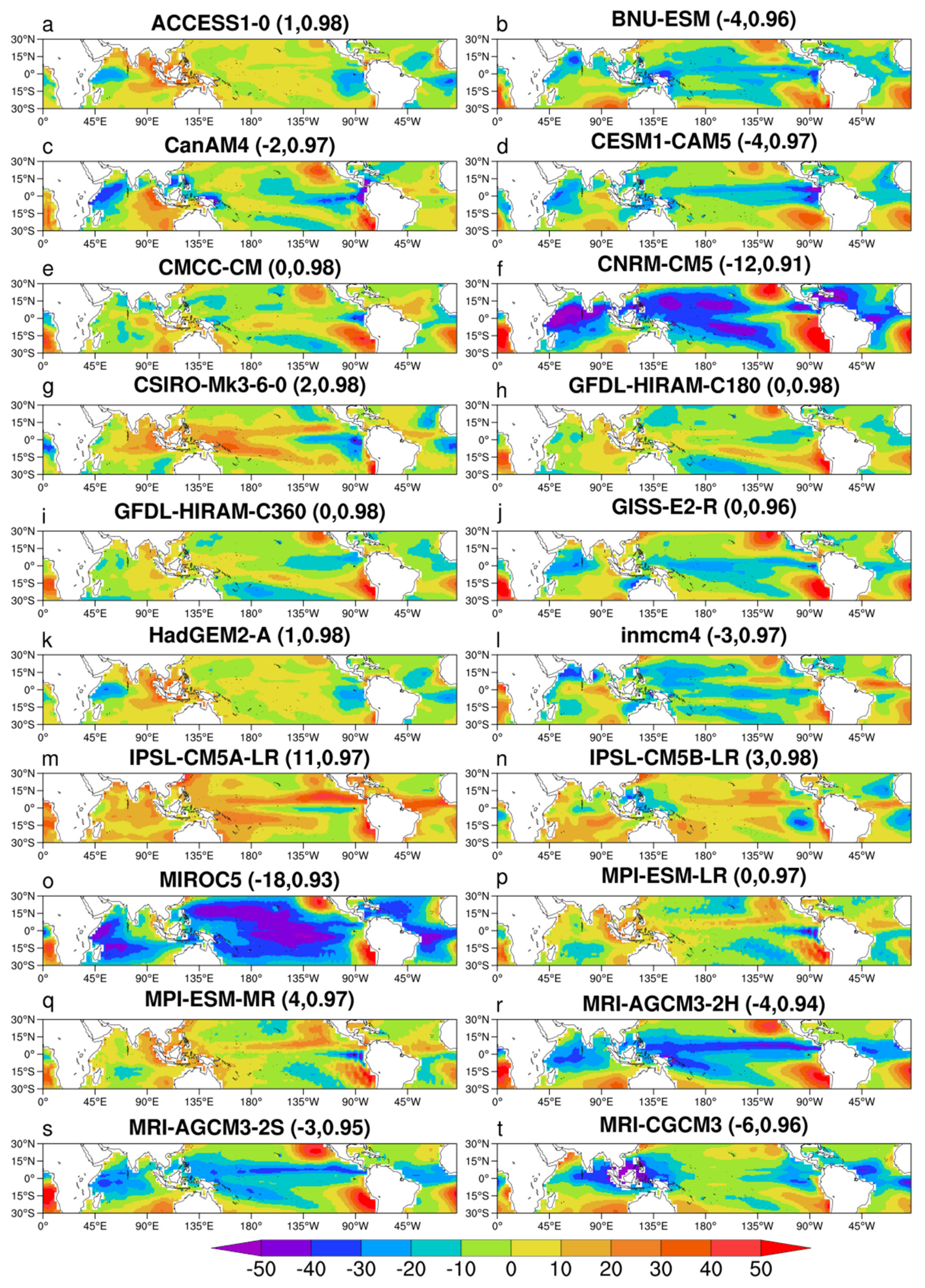
4.2. Shortwave (QSW)

Even though there is a systematic bias in QSW in all seasons (Figure 6, right), the correlation between the simulated and observed QSW is always above 0.9 (Table 1), which is also consistent with Loew et al. [14]. As was seen above for QLW, most of the bias in QSW also appears to come from bias in the cloud cover. For example, the model overestimates QSW in the southern Indian Ocean, where cloud cover shows a negative bias (comparing Figure 2f and Figure 9e). The bias in QSW is driven by bias in QDSW because QUSW is a function of QDSW and albedo (see Equations 3, 4). Since the QDSW is related to the cloud cover and vertical humidity structure in the atmosphere, among other factors, differences in QDSW are likely to be related to the model physics. For example, clouds enhance the planetary albedo by reflecting QDSW to space, leading to a cooling effect on the earth’s surface. Large bias in QSW in the southeast Pacific and southeast Indian Ocean (Figure 2f) is associated with the low-cloud cover (Figure 9f). This low cloud appears to be missing in the AMIP models due to prevalence of deep convection (and a lack of shallow convection) owing to cumulus parameterization that tends to produce high-level convective clouds. On the other hand, underestimation of QSW near the equator (Figure 2f) is over the region of high clouds (Figure 9b), and high clouds are likely overestimated in the model (Figure 9e). Probst et al. [50] also found a similar result. The relationship between the bias in QSW and total cloud cover (and precipitable water) was not performed (unlike QLW) due to unavailability of daytime data for cloud cover and precipitable water for AMIP simulations.

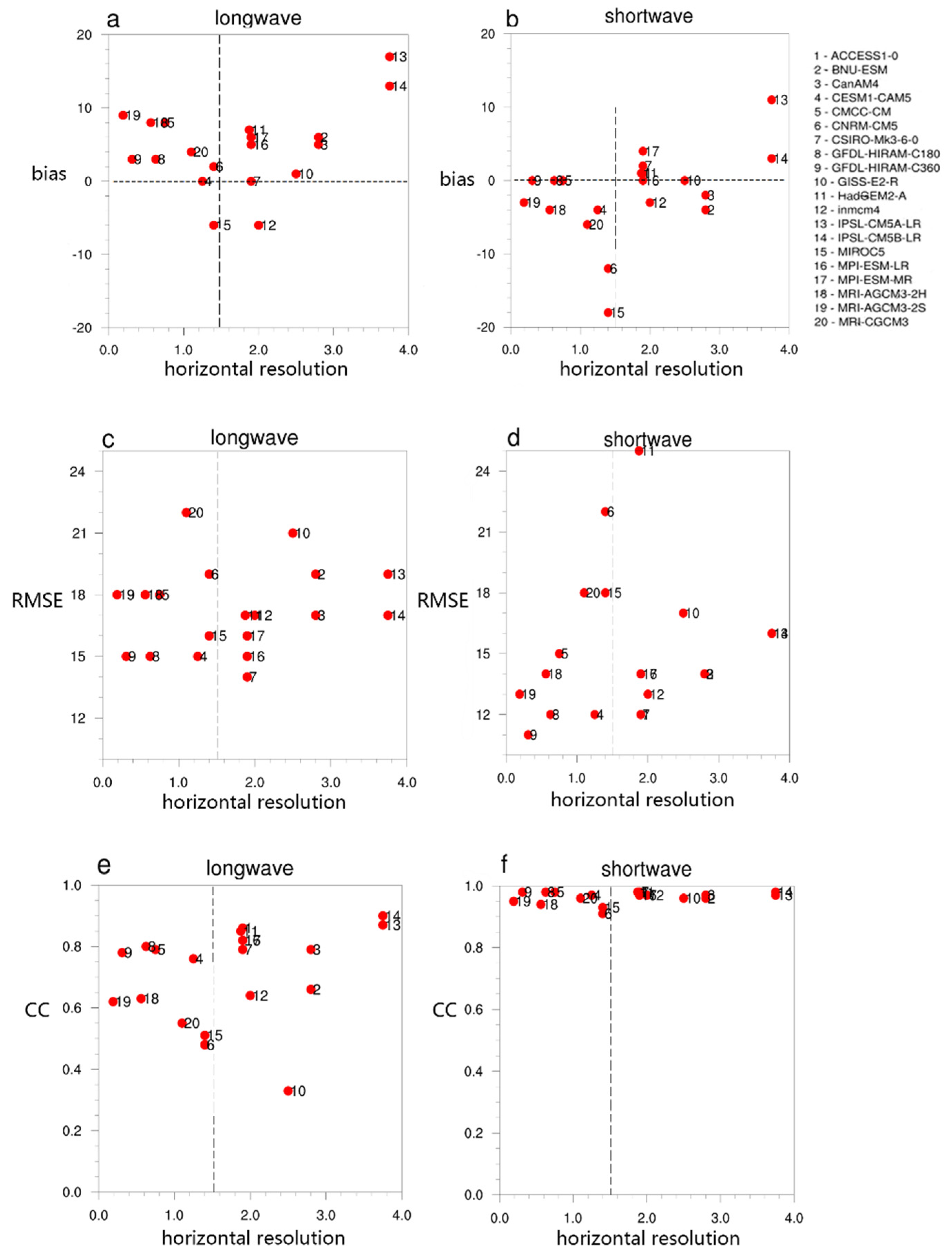
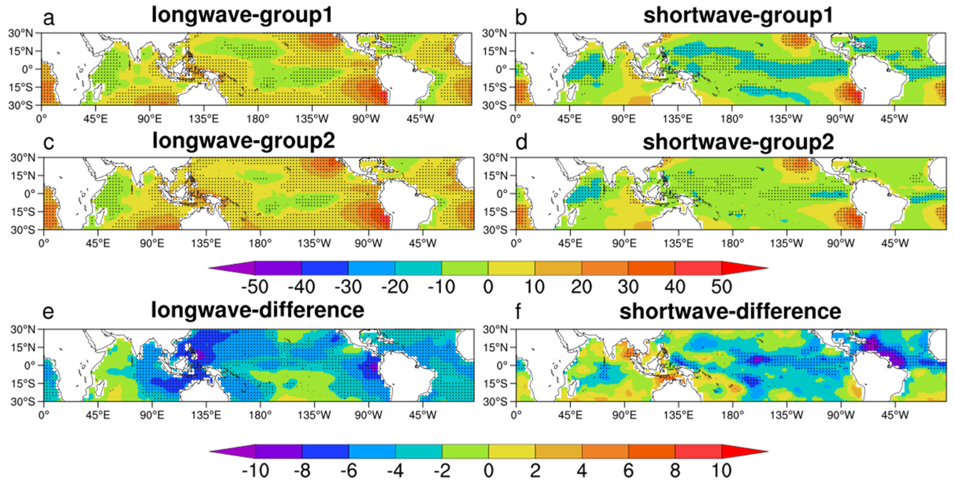
5. Dependence on Model Resolutions

The horizontal resolution of the model has been found to be an important factor in correctly simulating surface radiation (e.g., [10,12,15,52]). Therefore, we examine to what extent the spatio-temporal bias of surface radiative fluxes in the models is related to the horizontal resolutions of the models. This analysis is useful because it provides guidance when choosing a suitable resolution for a model, particularly since we found (e.g., Table 1, Figure 8) that some high-resolution models tend to simulate surface radiation better than others.
To quantify the possible role of the horizontal resolution of the models on the simulated surface radiation, we split the models into two groups: models with <1.5° horizontal grid spacing (group 1) and models with >1.5° horizontal grid spacing (group 2). The ACCESS1-0 (1.25° × 1.9°) and HadGEM2-A (1.25° × 1.875°) models were considered in group 1. Including these two models in group 2 changes the results only slightly. In general, the models in group 1 have lower bias and RMSE, and higher CC, than the models in group 2 (Table 3, Figure 12). The bias in QSW is larger in group 1 than group 2 due to a large bias in two group 1 models (CNRM-CM5 and MIROC5, Figure 12b) both of which have grid spacing of 1.4° × 1.4°. On the other hand, the bias in QLW (Figure 12a) in group 2 is primarily due to large biases in two models of the models of that group (IPSL-CM5A-LR and IPSL-CMPB-LR), both of which have grid spacing of 1.875° × 3.75°.
The overall slightly better performance of the high-resolution models than the coarse-resolution models may not be attributed entirely to the horizontal resolutions, because these models use different parameterization schemes (e.g., convection, radiation, and planetary boundary layer) that can cause differences in cloud cover, precipitable water, and surface radiative fluxes. As a result, to explore the influence of horizontal resolution, we need to compare results from models with the same parameterization packages but with different horizontal resolutions. There are only two such sets in our chosen models, one set consisting of two GFDL models and the other set consisting of three MRI models (Table 1). In both sets, higher resolution versions of the models perform better than their coarse resolution counterpart concerning RMSE (Table 1).
The influence of grid spacing on the spatial distribution of surface radiation bias is explored in Figure 13. In general, group 1 models perform slightly better than group 2 models, but systematic bias in the eastern Pacific, southeastern Atlantic, and the southeastern Indian Ocean persists in both group of models. For QSW (Figure 13b,d), the bias along the equator is reduced in group 1 models, possibly showing the importance of higher grid-spacing in correctly simulating surface radiation. In general, models in group 1 have a relatively higher correlation and lower deviations than models in group 2 (Table 3, Figure 8). However, the difference between high- and low-resolution models is statistically significant over most parts of the tropical oceans for QLW only (Figure 13e). For QSW (Figure 13f), the difference between the two groups is statistically significant only close to the equator, showing the influence of the high-level clouds in the ITCZ.

6. Summary and Conclusion

Surface radiation is a major constituent of the surface energy budget that influences the earth’s weather and climate. This study evaluates the ability of 20 models participating in AMIP to simulate the surface longwave (QLW) and shortwave (QSW) and explores several possible reasons behind model bias over the tropical oceans during 22 years (1979−2000). The main conclusions could be summarized as follows:
(1) For surface radiation, it is found that the western parts of the oceans generally have lower biases than eastern parts (Figure 2). This difference in bias is likely because of errors in cloud cover (e.g., [53]) in the simulations (Figure 9 and Figure 10) and is not surprising given that the GCMs with cumulus parameterization tend to underestimate low-level clouds over cooler SST (e.g., [49,53,54]). Zhang et al. [55] also found that cloud cover causes the largest uncertainty in the downwelling shortwave QDSW at the surface. The largest error comes from the coastal areas of off-equatorial eastern Pacific Ocean. The bias varies over different seasons with the highest bias during the boreal summer, but some systematic bias persists over all seasons (Figure 6, Table 2).
(2) The error in surface net longwave radiation QLW comes almost entirely from downwelling longwave QDLW. The bias in upwelling longwave QULW is minimal because QULW is dependent on the SST, and the SST was provided from the observations. The QDLW was underestimated in 16 out of 20 models. This result is consistent with Garratt and Prata [12] who also found that the QDLW is typically underestimated in GCMs. Clouds absorb and reemit longwave radiation back to the surface having a great impact on QDLW (e.g., [56]).
(3) The RMSE in QLW was larger than that in QSW in all models except CNRM-CM5, HADGEM2-A, and MIROC5 (Table 1). Interestingly, the correlation was higher for QSW than QLW in all 20 models (Table 3, Figure 8). To what extent these errors in radiation were related to the cumulus parameterizations of the models (e.g., May et al. 2012) or sampling biases (e.g., [57]) is left as an area of future work.
(4) Models with higher horizontal resolutions generally are slightly better at simulating surface radiation than models with lower horizontal resolutions (Figure 12 and Figure 13 and Table 3). English et al. [15] along with several other studies (e.g., [12,13]), also confirmed that the accuracy in surface radiative fluxes of any model is largely affected by its resolution. For example, the RMSE in high-resolution models for QLW and QSW was lower by 3 and 2 W m−2, respectively than in low-resolution models. Overall, GFDL-HIRAM-C180 and GFDL-HIRAM-C360 perform best for surface radiative fluxes. Interestingly, these two models used cumulus parameterization that includes shallow convection [58]. As a result, when the atmosphere is not sufficiently moist, deep convection can be inhibited to the extent that a significant portion of the precipitation is controlled by the large-scale, and not by the convection module [29].
In the model validation of surface radiation, apart from the observational uncertainty (see Section 2), there are also issues related to model uncertainty coming from the temporal frequency of the model output. Typically, model output was taken every six hours. As a result, in the presence of large variation in the diurnal cycle of cloudiness over the tropical oceans, there would be sampling biases for surface radiation. Even with these uncertainties in mind, the major implication of this study is that the models perform poorly over regions of shallow convection. As a result, cumulus parameterization in association with shallow convection scheme may be preferred to capture surface radiation in a model adequately. The net radiation at the surface is nearly balanced by the surface latent and sensible heat fluxes. Therefore, any error in the net surface radiation will invariably affect the surface latent and sensible heat fluxes. In particular, surface latent heat flux is associated with the surface evaporation, which is a component of the hydrological cycle and has important implications for society [59]. It would be interesting to find whether the AMIP simulations in the forthcoming CMIP6 models can capture the surface radiation better than AMIP simulations from CMIP5 models.
In summary, the AMIP simulations were able to capture the spatial distribution of surface radiation, although with systematic biases, in particular, in the regions of low-level clouds. The bias was larger for QLW than QSW, even though the absolute magnitude of QLW is much smaller than QSW. The higher resolution models performed slightly better than lower resolution models for both QLW and QSW. Two high-resolution GFDL models with a parameterization for shallow convection outperform the ensemble mean. The models that perform best over the tropics overall may not be best over a particular region. As a result, care must be taken to choose a model or a set of models when applied to a specific area in the tropics.

Author Contributions

Conceptualization, P.R. and X.Z.; methodology, All; formal analysis, X.Z.; writing—original draft preparation, X.Z and P.R.; writing—review and editing, All; visualization, X.Z.; supervision, P.R.; funding acquisition, P.R.

Funding

This research was funded by grants from the NSF (1323400) and the ONR (N00014–1601-3091) to PR and ONR (N00014-16WX-01752) to BB.

Acknowledgments

The surface heat flux data was taken from the WHOI OAFlux project (http://oaflux.whoi.edu, last access: 6 November 2018) which was funded by the NOAA Climate Observations and Monitoring program. The ISCCP cloud data was taken from https://isccp.giss.nasa.gov/products/browsed2.html We also thank the climate modeling groups who participated in AMIP for producing and making available their model output. The tropical moored buoy arrays are supported by NOAA’s Climate Program Office. ISCCP data were obtained from the NASA Langley Research Center Atmospheric Sciences Data Center.

Conflicts of Interest

The authors declare no conflict of interest. The funders had no role in the design of the study; in the collection, analyses, or interpretation of data; in the writing of the manuscript, or in the decision to publish.

References

  1. Jiang, C.; Cronin, M.F.; Kelly, K.A.; Thompson, L. Evaluation of a hybrid satellite and NWP-based turbulent heat flux product using Tropical Atmosphere-Ocean (TAO) buoys. J. Geophys. Res. 2005, 110, C09007. [Google Scholar] [CrossRef]
  2. Trenberth, K.E.; Caron, J.M.; Stepaniak, D.P.; Worley, S. Evolution of El Niño–Southern Oscillation and global atmospheric surface temperatures. J Geophys. Res. (Atmos.) 2002, 107, AAC 5-1–AAC 5-17. [Google Scholar] [CrossRef]
  3. Kiehl, J.T.; Trenberth, K.E. Earth’s Annual Global Mean Energy Budget. Bull. Am. Meteorol. Soc. 1997, 78, 197–208. [Google Scholar] [CrossRef]
  4. Stephens, G.L.; L’Ecuyer, T. The earth’s energy balance. Atmos. Res. 2015, 166, 195–203. [Google Scholar] [CrossRef]
  5. Gates, W.L. An overview of the results of the Atmospheric Model Intercomparison Project (AMIP 1). Bull. Am. Meteorol. Soc. 1999, 80, 29–56. [Google Scholar] [CrossRef]
  6. Bisht, G.; Venturini, V.; Islama, S.; Jiang, L. Estimation of the net radiation using MODIS (Moderate Resolution Imaging Spectroradiometer) data for clear sky days. Remote Sens. Environ. 2005, 97, 52–67. [Google Scholar] [CrossRef]
  7. Li, J.-L.F.; Waliser, D.E.; Stephens, G.; Lee, S.; L’Ecuyer, T.; Kato, S.; Loeb, N.; Ma, H.Y. Characterizing and understanding radiation budget biases in CMIP3/CMIP5 GCMs, contemporary GCM, and reanalysis. J. Geophys. Res. 2013, 118, 8166–8184. [Google Scholar] [CrossRef]
  8. Klein, S.A.; Zhang, Y.; Zelinka, M.D.; Pincus, R.N.; Boyle, J.; Gleckler, P.J. Are climate model simulations of clouds improving? An evaluation using the ISCCP simulator. J. Geophys. Res. 2012, 118, 1329–1342. [Google Scholar] [CrossRef]
  9. Wild, M.; Ohmura, A.; Gilgne, H.; Morcrette, J.J.; Slingo, A. Evaluation of downward longwave radiation in general circulation models. Bull. Am. Meteorol. Soc. 2001, 11, 3227–3239. [Google Scholar] [CrossRef]
  10. Garratt, M.; Ohmura, A.; Gilgen, H. validation of general circulation model simulated surface radiative fluxes using surface measurements from the Global Energy Balance Archive. J. Clim. 1995, 8, 1309–1324. [Google Scholar]
  11. Allen, R.J.; Norris, J.R.; Wild, M. Evaluation of multidecadal variability in CMIP5 surface solar radiation and inferred underestimation of aerosol direct effects over Europe, China, Japan, and India. J. Geophys. Res. Atmos. 2013, 118, 6311–6336. [Google Scholar] [CrossRef]
  12. Garratt, J.R.; Prata, A.J. Downwelling longwave fluxes at continental surface—A comparison with GCM simulations and implications for the global land-surface radiation bufget. J. Clim. 1996, 9, 646–655. [Google Scholar] [CrossRef]
  13. Wild, M.; Folini, D.; Hakuba, M.Z.; Schär, C.; Seneviratne, S.I.; Kato, S.; Rutan, D.; Ammann, C.; Wood, E.F.; König-Langlo, G. The energy balance over land and oceans: an assessment based on direct observations and CMIP5 climate models. Clim. Dyn. 2015, 44, 3393–3429. [Google Scholar] [CrossRef]
  14. Loew, A.; Andersson, A.; Trentmann, J.; Schröder, M. Assessing surface solar radiation fluxes in the CMIP ensembles. J. Clim. 2016, 29, 7231–7246. [Google Scholar] [CrossRef]
  15. English, J.M.; Gettelman, A.; Henderson, G.R. Arctic Radiative Fluxes: Present-Day Biases and Future Projections in CMIP5 Models. J. Clim. 2015, 28, 6019–6038. [Google Scholar] [CrossRef]
  16. Taylor, K.E.; Ronald, J.; Meehl, G.A. An overview of CMIP5 and the experiment design. Bull. Am. Meteorol. Soc. 2012, 28, 485–498. [Google Scholar] [CrossRef]
  17. Fiorino, M. AMIP II Sea Surface Temperature and Sea Ice Concentration observations. PCMDI Rep. 2000, 60. Available online: https://pcmdi.llnl.gov/mips/amip/amip2/ (accessed on 1 October 2019).
  18. Rossow, W.B.; Walker, A.W.; Beuschel, D.E.; Roiter, M.D. International Satellite Cloud Climatology Project (ISCCP) documentation of new cloud datasets. WMO/TD-No. 737; World Meteorological Organization: Geneva, Switzerland, 1996; p. 115. Available online: https://isccp.giss.nasa.gov/pub/documents/d-doc.pdf (accessed on 1 October 2019).
  19. Yu, L.S.; Jin, X.Z.; Weller, R.A. Multidecade Global Flux Datasets from the Objectively Analyzed Air-sea Fluxes (OAFlux) Project: Latent and Sensible Heat Fluxes, Ocean Evaporation, and Related Surface Meteological Variables; OAFlux Project Technical Report; Woods Hole Oceanographic Institution: Woods Hole, MA, USA, 2008. [Google Scholar]
  20. Schiffer, R.A.; Rossow, W.B. ISCCP global radiance data set: A new resource for climate research. Bull. Am. Meteorol. Soc. 1985, 66, 1498–1505. [Google Scholar] [CrossRef]
  21. Rossow, W.B.; Schiffer, R.A. Advances in understanding clouds from ISCCP. Bull. Am. Meteorol. Soc. 1999, 80, 2261–2288. [Google Scholar] [CrossRef]
  22. Dix, M.; Vohralik, P.; Bi, D.; Rashid, H.; Marsland, S.; O’Farrell, S.; Uotila, P.; Hirst, T.; Kowalczyk, E.; Sullivan, A.; et al. The ACCESS couple model: documentation of core CMIP5 simulations and initial results. Aust. Met. Oceanogr. J. 2013, 63, 83–99. [Google Scholar] [CrossRef]
  23. Ji, D.; Wang, L.; Feng, J.; Wu, Q.; Cheng, H.; Zhang, Q.; Yang, J.; Dong, W.; Dai, Y.; Gong, D.; et al. Description and basic evaluation of Beijing Normal University Earth System Model (BNU-ESM) version 1. Geosci. Model Dev. 2014, 7, 2039–2064. [Google Scholar] [CrossRef] [Green Version]
  24. Von Salzen, K.; Scinocca, J.F.; McFarlane, N.A.; Li, J.; Cole, J.N.S.; Plummer, D.; Verseghy, D.; Reader, M.C.; Ma, X.; Lazare, M.; et al. The Canadian fourth generation atmospheric global climate model (CanAM4). Part I: Representation of physical processes. Atmos. Ocean. 2013, 51, 104–125. [Google Scholar] [CrossRef]
  25. Meehl, G.A.; Washington, W.M.; Arblaster, J.M. Climate change projections in CESM1(CAM5) compared to CCSM4. J. Clim. 2013, 26, 6287–6308. [Google Scholar] [CrossRef]
  26. Scoccimarro, E.; Gualdi, S.; Bellucci, A.; Sanna, A.; Fogli, P.G.; Manzini, E.; Vichi, M.; Oddo, P.; Nabarra, A. Effects of tropical cyclones on ocean heat transport in a high-resolution coupled general circulation model. J. Clim. 2011, 24, 4368–4384. [Google Scholar] [CrossRef]
  27. Voldoire, A.; Sanchez-Gomez, E.; Salasymelia, D.; Decharme, B.; Cassou, C.; Senesi, S.; Valcke, S.; Beau, I.; Alias, A.; Chevallier, M.; et al. The CNRM-CM5.1 global climate model: description and basic evaluation. Clim. Dyn. 2013, 40, 2091–2121. [Google Scholar] [CrossRef]
  28. Rotstayn, L.D.; Jeffrey, S.J.; Collier, M.A.; Dravitzki, S.M.; Hirst, A.C.; Syktus, J.I.; Wong, K.K. Aerosol- and greenhouse gas-induced changes in summer rainfall and circulation in the Australasian region: a study using single-forcing climate simulations. Atmos. Chem. Phys. 2012, 12, 6377–6404. [Google Scholar] [CrossRef] [Green Version]
  29. Zhao, M.; Held, I.M.; Lin, S.J.; Vecchi, J.A. Simulations of global hurricane climatology, interannual variability, and response to global warming using a 50-km resolution GCM. J. Clim. 2009, 22, 6653–6678. [Google Scholar] [CrossRef]
  30. Schmidt, G.A.; Ruedy, R.; Hansen, J.E.; Aleinov, I.; Bell, N.; Bauer, M.; Bauer, S.; Cairns, B.; Canuto, V.; Cheng, Y.; et al. Present-day atmospheric simulations using GISS model: Comparison to in situ, satellite, and reanalysis data. J. Clim. 2006, 19, 153–192. [Google Scholar] [CrossRef]
  31. Martin, G.M.; Bellouin, N.; Collins, W.J.; Culverwell, I.D. The HadGEM2 family of Met Office Unified Model Climate configurations. Geosci. Model Dev. 2011, 4, 723–757. [Google Scholar]
  32. Volodin, E.M.; Dianskii, N.A.; Gusev, A.V. Simulating present-day climate with the INMCM4.0 coupled model of the atmospheric and oceanic general circulations. IZV. Atmos. Ocean. Pgys. 2010, 46, 414–431. [Google Scholar]
  33. Dufresne, J.L.; Foujols, M.A.; Denvil, S.; Caubel, A.; Marti, O.; Aumont, O.; Balkanski, Y.; Bekki, S.; Bellenger, H.; Benshila, R.; et al. Climate change projections using the IPSL-CM5 Earth System Model: From CMIP3 to CMIP5. Clim. Dyn. 2013, 40, 2123–2165. [Google Scholar] [CrossRef]
  34. Hourdin, F.; Grandpeix, J.Y.; Rio, C.; Bony, S.; Jam, A.; Cheruy, F.; Rochetin, N.; Fairhead, L.; Idelkadi, A.; Musat, I.; et al. LMDZ5B: the atmospheric component of the IPSL climate model with revisited parameterizations for clouds and convection. Clim. Dyn. 2013, 40, 2193–2222. [Google Scholar] [CrossRef]
  35. Watanabe, M.; Suzuki, T.; O’ishi, R.; Komuro, Y.; Watanabe, S.; Emori, S.; Takemura, T.; Chikira, M.; Ogura, T.; Sekiguchi, M.; et al. Improved Climate Simulation by MIROC5: Mean States, Variability, and Climate Sensitivity. J. Clim. 2010, 23, 6312–6335. [Google Scholar] [CrossRef]
  36. Stevens, B.; Giorgetta, M.; Esch, M.; Mauritsen, T.; Crueger, T.; Rast, S.; Salzmann, M.; Schmidt, H.; Bader, J.; Block, K.; et al. Atmospheric component of the MPI-M earth system model: ECHAM6. J. Adv. Model. Earth Syst. 2013, 5, 146–172. [Google Scholar] [CrossRef]
  37. Mizuta, R.; Yoshimura, H.; Murakami, H.; Matsueda, M.; Endo, H.; Ose, T.; Kamiguchi, K.; Hosaka, M.; Sugi, M.; Yukimota, S.; et al. Climate simulations using MRI-AGCM3.2 with 20-km Grid. J. Meteor. Soc. Jpn. 2012, 90, 233–258. [Google Scholar] [CrossRef]
  38. Yukimoto, S.; Adachi, Y.; Hosaka, M.; Sakami, T.; Yoshimura, H.; Hirabara, M.; Tanaka, T.Y.; Shindo, E.; Tsujino, H.; Deushi, M.; et al. A new global climate model of the meteorological research institute: MRI-CGCM3. J. Meteorol. Soc. 2012, 90, 23–64. [Google Scholar] [CrossRef]
  39. Cronin, M.F.; Fairall, C.W.; McPhaden, M.J. An assessment of buoy-derived and numerical weather prediction surface heat fluxes in the tropical Pacific. J. Geophys. Res. 2006, 111, C0603. [Google Scholar] [CrossRef]
  40. Cole, J.; Barker, H.W.; Loeb, N.G.; Von Salzen, K. Assessingsimulated clouds and radiativefluxes using properties of clouds whose topsare exposed to space. J. Clim. 2011, 24, 2715–2727. [Google Scholar] [CrossRef]
  41. Zhang, Y.-C.; Rossow, W.B.; Lacis, A.A.; Oinas, V.; Mishchenko, M.I. Calculation of radiative fluxes from the surface to top of atmosphere based on ISCCP and other global data sets: Refinements of the radiative transfer model and the input data. J. Geophys. Res. 2004, 109, D19105. [Google Scholar] [CrossRef]
  42. Pinker, R.T.; Bentamy, A.; Katsaros, K.B.; Ma, Y.; Li, C. Estimates of net heat fluxes over the Atlantic Ocean. J. Geophys. Res. 2014, 119, 410–427. [Google Scholar] [CrossRef]
  43. Ray, P.; Zhang, C.; Dudhia, J.; Li, T.; Moncrieff, M.W. Tropical channel model. In Climate Models; Druyan, L.M., Ed.; IntechOpen: London, UK, 2012; pp. 3–18. ISBN 978-953-308-181-6. [Google Scholar]
  44. Tan, H.; Ray, P.; Barrett, B.S.; Tewari, M.; Moncrieff, M.W. Role of topography on the MJO in the Maritime Continent: a numerical case study. Clim. Dyn. 2018, 1–20. [Google Scholar] [CrossRef]
  45. Wallcraft, A.J.; Kara, A.B.; Hurlburt, H.E.; Chassignet, E.P.; Halliwell, G.H. Value of bulk heat flux parameterizations for ocean SST prediction. J. Mar. Syst. 2008, 74, 241–258. [Google Scholar] [CrossRef]
  46. Zhang, T.; Stackhouse, P.W.; Gupta, S.K.; Cox, S.J.; Mikovitz, J.C.; Hinkelman, L.M. The validation of the GEWEX SRB surface shortwave flux data products using BSRN measurements: A systematic quality control, production and application approach. J. Quant. Spectrosc. Radiat. Transfer. 2013, 122, 127–140. [Google Scholar] [CrossRef]
  47. May, J.C.; Barron, C.N. NFLUX satellite-based radiative heat fluxes. Part I: Swath-level products. J. Appl. Meteor. Climatol. 2017, 56, 1025–1041. [Google Scholar] [CrossRef]
  48. Weare, B.C. A comparison of AMIP II model cloud layer properties with ISCCP D2 estimates. Clim. Dyn. 2004, 22, 281–292. [Google Scholar] [CrossRef]
  49. Soden, B.J.; Vecchi, G.A. The vertical distribution of cloud feedback in coupled ocean-atmosphere models. Geophys. Res. Lett. 2011, 38, L12704. [Google Scholar] [CrossRef]
  50. Probst, P.; Rizzi, R.; Tosi, E.; Lucarini, V.; Maestri, T. Total cloud cover from satellite observations and climate models. Atmos. Res. 2012, 107, 161–170. [Google Scholar] [CrossRef]
  51. Huber, M.; Mahlstein, I.; Wild, M.; Fasullo, J.; Knutti, R. Constraints on Climate Sensitivity from Radiation Patterns in Climate Models. J. Clim. 2011, 24, 1034–1052. [Google Scholar] [CrossRef] [Green Version]
  52. Calisto, M.; Folini, D.; Wild, M.; Bengtsson, L. Cloud radiative forcing intercomparison between fully coupled CMIP5 models and CERES satellite data. Ann. Geophys. 2014, 32, 793–807. [Google Scholar] [CrossRef] [Green Version]
  53. Wyant, M.C.; Wood, R.; Bretherton, C.S.; Mechoso, C.R.; Bacmeister, J.; Balmaseda, M.A.; Barrett, B.; Codron, F.; Earnshaw, P.; Fast, J.; et al. The PreVOCA experiment: modeling the lower troposphere in the Southeast Pacific. Atmos. Chem. Phys. 2009, 10, 4757–4774. [Google Scholar] [CrossRef]
  54. Bony, S.; Dufresne, J.L. Marine boundary layer clouds at the heart of tropical cloud feedback uncertainties in climate models. Geophys. Res. Lett. 2005, 32, L20806. [Google Scholar] [CrossRef]
  55. Zhang, Y.C.; Rossow, W.B.; Lacis, A.A. Calculation of surface and top of atmosphere radiative fluxes from physical quantities based on ISCCP data sets: 1. Method and sensitivity to input data uncertainties. J. Geophys. Res. 1995, 100, 1149–1165. [Google Scholar] [CrossRef]
  56. Kratz, D.P.; Gupta, S.K.; Wilber, A.C.; Sothcott, V.E. Validation of the CERES edition 2B surface-only flux algorithms. J. Appl. Meteor. Climatol. 2010, 49, 164–180. [Google Scholar] [CrossRef]
  57. Weare, B.C.; Strub, P.T. The significance of sampling biases on calculated monthly mean oceanic surface heat flux. Tellus 1981, 33, 211–224. [Google Scholar] [CrossRef]
  58. Bretherton, C.S.; McCaa, J.R.; Grenier, H.A. New parameterization for shallow cumulus convection and its application to marine subtropical cloud-topped boundary layers. Part I: Description and 1D results. Mon. Weather Rev. 2004, 132, 864–882. [Google Scholar] [CrossRef]
  59. McNeeley, S.M.; Tessendorf, S.A.; Lazrus, H.; Heikkila, T.; Ferguson, I.M.; Arrigo, J.S.; Attari, S.Z.; Cianfrani, C.; Dilling, L.; Gurdak, J.; et al. Catalyzing frontiers in water-climate-society research: A view from early career scientists and junior faculty. Bull. Am. Meteorol. Soc. 2012, 93, 477–484. [Google Scholar] [CrossRef]
Figure 1. The locations of RAMA (Indian Ocean), TAO (Pacific Ocean), and PIRATA (Atlantic Ocean) moored buoys in the tropical oceans that were used for this study.
Atmosphere 10 00606 g001
Figure 2. (left) Climatological average of the QLW from (a) model ensemble, (c) OAFlux and (e) model ensemble minus OAFlux. Right panels are for QSW. Dotted areas in the bottom panels indicate where the bias is statistically significant at the 95% level based on a Student’s t-test. (unit: W m−2).
Atmosphere 10 00606 g002
Figure 3. Mean bias in the net surface longwave QLW estimated as a model minus the OAFLux over the tropical oceans. The numbers in the parentheses show the mean bias and correlation coefficient. (unit: W m−2).
Atmosphere 10 00606 g003
Figure 4. Mean bias in the net surface shortwave QSW estimated as model minus OAFLux over the tropical oceans. The numbers in the parentheses show the mean bias and correlation coefficient. (unit: W m−2).
Atmosphere 10 00606 g004
Figure 5. Latitudinal distribution of bias (model ensemble minus OAFLux) in QLW (red solid line) and QSW (blue dotted line) in the (a) Indian (40° E–100° E), (b) Pacific (100° E–80° W), and (c) Atlantic (80° W–10° E) oceans. (unit: w m−2).
Atmosphere 10 00606 g005
Figure 6. Seasonal mean bias of the model ensemble in (left) longwave (QLW) and (right) shortwave (QSW). Dotted areas indicate where the bias is statistically significant at the 95% level. (unit: W m−2).
Atmosphere 10 00606 g006
Figure 7. The annual cycle of (a) QSW and (b) QLW at the TAO buoys in the Pacific, (c) QSW at the PIRATA buoys in the Atlantic, and (d) QSW at the RAMA buoys in the Indian Ocean using data from 1997 to 2008. QLW at the RAMA and PIRATA locations were not plotted because of insufficient data from the buoys during this period. (unit: W m−2).
Atmosphere 10 00606 g007
Figure 8. Taylor diagrams showing the (a) climatological and (b,c) seasonal (DJF and JJA) mean bias of QLW and QSW along with related variables including the total cloud cover (cl), and total precipitable water (TPW) simulated by 20 AMIP models compared to OAFlux from 1979 to 2000. The numbers 1 to 20 represent 20 AMIP models.
Atmosphere 10 00606 g008
Figure 9. (left) Total cloud cover (%) from the model ensemble (a), observation (c) and bias (e) (model ensemble minus observation). (right) High- (b), mid- (d), and low-level (f) clouds (%) from the ISCCP data. Dotted areas indicate where the bias is statistically significant at the 95% level.
Atmosphere 10 00606 g009
Figure 10. Relationship between bias in the total cloud cover (%) and bias in QLW (W m−2) over the (a) Indian (40° E–100° E), (b) Atlantic (70° W–10° E), (c) western Pacific (100° E–160° E), and (d) eastern Pacific Oceans (120°–70° W) during December-January-February (DJF, red) and June-July-August (JJA, green).
Atmosphere 10 00606 g010
Figure 11. Relationship between bias in the total precipitable water TPW (Kg m−2) and bias in QLW (W m−2) over the (a) Indian (40° E–100° E), (b) Atlantic (70° W–10° E), (c) western Pacific (100° E–160° E), and (d) eastern Pacific Oceans (120°–70° W) during DJF (red) and JJA (green).
Atmosphere 10 00606 g011
Figure 12. (top) Distribution of horizontal resolution (in °) and bias (W m−2) from 20 models over 30° S to 30° N from 1979 to 2000 for (a) longwave QLW and (b) shortwave QSW. The middle (c,d) and bottom (e,f) panels are for RMSE (W m−2) and CC, respectively.
Atmosphere 10 00606 g012
Figure 13. (left) Bias in QLW of (a) group 1 models (<1.5° resolution ), (c) group 2 models (>1.5° resolution ), and (e) their differences. Right panels (b,d,f) are for QSW. Dotted areas at the bottom panels indicate where the difference is statistically significant at the 95% level. Unit: W m−2.
Atmosphere 10 00606 g013
Table 1. Description of the 20 Atmospheric Model Intercomparison Project (AMIP) models used for this study along with the primary references. The bias and root mean squared error (RMSE, averaged over 30° S–30° N) are written to the closest W m−2. CC stands for the correlation coefficient.
No.ModelHorizontal Resolution
Lat × Lon (No of Levels)
ReferencesQLWQSW
BiasRMSECCBiasRMSECC
1ACCESS1-01.25° × 1.9° (38)[22]6160.861120.98
2BNU-ESM2.8° × 2.8° (26)[23]6190.66−4140.96
3CanAM42.8° × 2.8° (26)[24]5170.79−2140.97
4CESM1-CAM50.94° × 1.25° (27)[25]0150.76−4120.97
5CMCC-CM0.75° × 0.75° (31)[26]8180.790150.98
6CNRM-CM51.4° × 1.4° (27)[27]2190.48−12220.91
7CSIRO-Mk3-6-01.9° × 1.9° (18)[28]0140.792120.98
8GFDL-HIRAM-C1800.5° × 0.625° (48)[29]3150.800120.98
9GFDL-HIRAM-C3600.25° × 0.31° (48)[29]3150.780110.98
10GISS-E2-R2° × 2.5° (40)[30]1210.330170.96
11HadGEM2-A1.25° × 1.875° (60)[31]7170.851250.98
12INM-CM41.5° × 2° (21)[32]−6170.64−3130.97
13IPSL-CM5A-LR1.875° × 3.75° (39)[33]17190.8711160.97
14IPSL-CM5B-LR1.875° × 3.75° (39)[34]13170.903160.98
15MIROC51.4° × 1.4° (40)[35]−6160.51−18180.93
16MPI-ESM-LR1.9° × 1.9° (26)[36]5150.820140.97
17MPI-ESM-MR1.9° × 1.9° (26)[36]6160.824140.97
18MRI-AGCM3-2H0.56° × 0.56° (48)[37]8180.63−4140.94
19MRI-AGCM3−2S0.19° × 0.19° (48)[37]9180.62−3130.95
20MRI-CGCM31.1° × 1.1° (48)[38]4220.55−6180.96
Model ensemble 4160.73−4140.97
Table 2. The seasonal and annual mean of QLW and QSW from the model ensemble and their bias compared to the OAFlux (1979–2000) and moored buoys (1997–2008). Comparison with the OAFlux was made over 30° S–30° N and 10° S–10° N (parentheses). The values were written to the closest W m−2.
Seasons DJFMAMJJASONAnnual
Qsurf ModelObsBiasModelObsBiasModelObsBiasModelObsBiasModelObsBias
Comparison with OAFlux
QLW5855359536575165552357534
(55)(53)(2)(57)(52)(5)(54)(51)(3)(51)(49)(2)(55)(51)(4)
QSW226230−4216219−3212216−4217224−7218222−4
(226)(235)(−9)(223)(227)(−4)(220)(224)(−4)(229)(238)(−9)(225)(231)(−6)
Qnett2252−301448−341452−382151−281950−31
(37)(61)(−24)(31)(57)(−26)(35)(55)(−20)(50)(72)(−22)(38)(63)(−25)
Comparison with Buoy data
QLW5453157543565245752556533
QSW227231−4213218−5214219−5211221−10216222−6
Table 3. Climatological bias, RMSE and CC (correlation) of QLW and QSW for high resolution (group 1 < 1.5°) and low-resolution (group 2 > 1.5°) models. A comparison was made over 30° S–30° N and 10° S–10° N (parentheses). The bias and RMSE were written to the closest W m−2.
ModelQLWQSW
BiasRMSECCBiasRMSECC
Group 1 (<1.5°)3 (3)16 (13)0.71 (0.74)−4 (−6)14 (17)0.96 (0.97)
Group 2 (>1.5°)5 (6)18 (16)0.73 (0.75)1 (−5)16 (21)0.96 (0.96)

