Article

Linearizations of the Spherical Harmonic Discrete Ordinate Method (SHDOM)

Remote Sensing Technology Institute, German Aerospace Center (DLR), 82234 Oberpfaffenhofen, Germany
*
Author to whom correspondence should be addressed.
Atmosphere 2019, 10(6), 292; https://doi.org/10.3390/atmos10060292
Submission received: 23 April 2019 / Revised: 21 May 2019 / Accepted: 22 May 2019 / Published: 28 May 2019
(This article belongs to the Special Issue Radiative Transfer Models of Atmospheric and Cloud Properties)

Abstract

:
Linearizations of the spherical harmonic discrete ordinate method (SHDOM) by means of a forward and a forward-adjoint approach are presented. Essentially, SHDOM is specialized for derivative calculations and radiative transfer problems involving the delta-M approximation, the TMS correction, and the adaptive grid splitting, while practical formulas for computing the derivatives in the spherical harmonics space are derived. The accuracies and efficiencies of the proposed methods are analyzed for several test problems.

1. Introduction

Accurate and efficient modeling of radiative transfer is important for the retrieval of earth atmospheric constituent information by means of remote sensing. Real clouds are an inhomogeneous three-dimensional scattering medium. For the new generation of satellite spectrometers with a relative high spatial resolution (such as Sentinel 5 Precursor, Sentinel 4 and Sentinel 5 [1]), it is important to account for the sub-pixel cloud inhomogeneities, or at least, to assess their effect on the radiances at the top of the atmosphere, and in particular, on the trace gas and cloud retrieval results. So far, the majority of operational retrieval algorithms are based on the one-dimensional (1D) radiative transfer model, which neglects all horizontal variability of the atmosphere. However, 1D approximation can lead to the significant errors in the calculated radiances and retrieved parameters [2,3,4,5,6]. In this regard, three-dimensional (3D) radiative trasnfer models are required.
The SHDOM method developed by Evans is a widely used deterministic method to solve the 3D radiative transfer equation [7]. The radiative transfer equation is solved iteratively by using the spherical harmonic and the discrete ordinate representations of the radiance field. Each iteration consists of four steps: (1) the transformation of the source function from spherical harmonics to discrete ordinates; (2) the integration of the source function along discrete ordinate directions to compute the radiance field; (3) the transformation of the discrete ordinate radiances to spherical harmonics; and (4) the calculation of the source function from the radiance in spherical harmonics space. An important feature of SHDOM is the adaptive grid technique. This technique improves the solution accuracy by increasing the spatial resolution in regions where the source function is changing more rapidly. The difference scheme employed in SHDOM is a characteristic scheme. In the so-called long characteristic method, the integration is performed along the whole characteristic of the differential operator, while in the short characteristic method, the integration is performed along a segment of the characteristic located inside a cell. SHDOM has been modfied for use on multiple processors [8], and to include polarization [9,10,11].
In atmospheric remote sensing and data assimilation, it is necessary to compute the partial derivatives of the outgoing radiances with respect to some atmospheric parameters of interest. For this purpose, a linearized forward approach, relying on an analytical computation of the derivatives, or a linearized forward-adjoint approach, relying on the application of the adjoint radiative transfer theory, can be used. For a plane-parallel geometry, scalar and vector linearized forward approaches were described in Refs. [12,13], while linearized forward-adjoint approaches were proposed in [14,15,16,17,18,19,20,21]. The forward-adjoint method is extremely efficient because only two radiative transfer calculations are required for derivatives calculations.
A theoretical framework for three-dimensional remote sensing of the atmosphere with adjoint methods was described by Martin et al. [22]. In a subsequent paper, Martin and Hasekamp [23] used the linearized-forward approach to retrieve cloud extinction fields from multi-angle measurements. Although, the analysis was restricted to two-dimensional problems (a two-dimensional domain and a set of directions confined to the unit circle and characterized by one angular variable), the efficiency of adjoint methods for multi-dimensional remote sensing of the atmosphere and surface was demonstrated.
In this paper, linearizations of SHDOM by using a forward and a forward-adjoint approach are presented. After formulating the problem in Section 2, we discuss in Section 3 the fundamentals of the linearized SHDOM with a forward-adjoint approach. The accuracy and efficiency of the linearized models is analyzed in Section 4, while the final section of our paper contains a few concluding remarks.

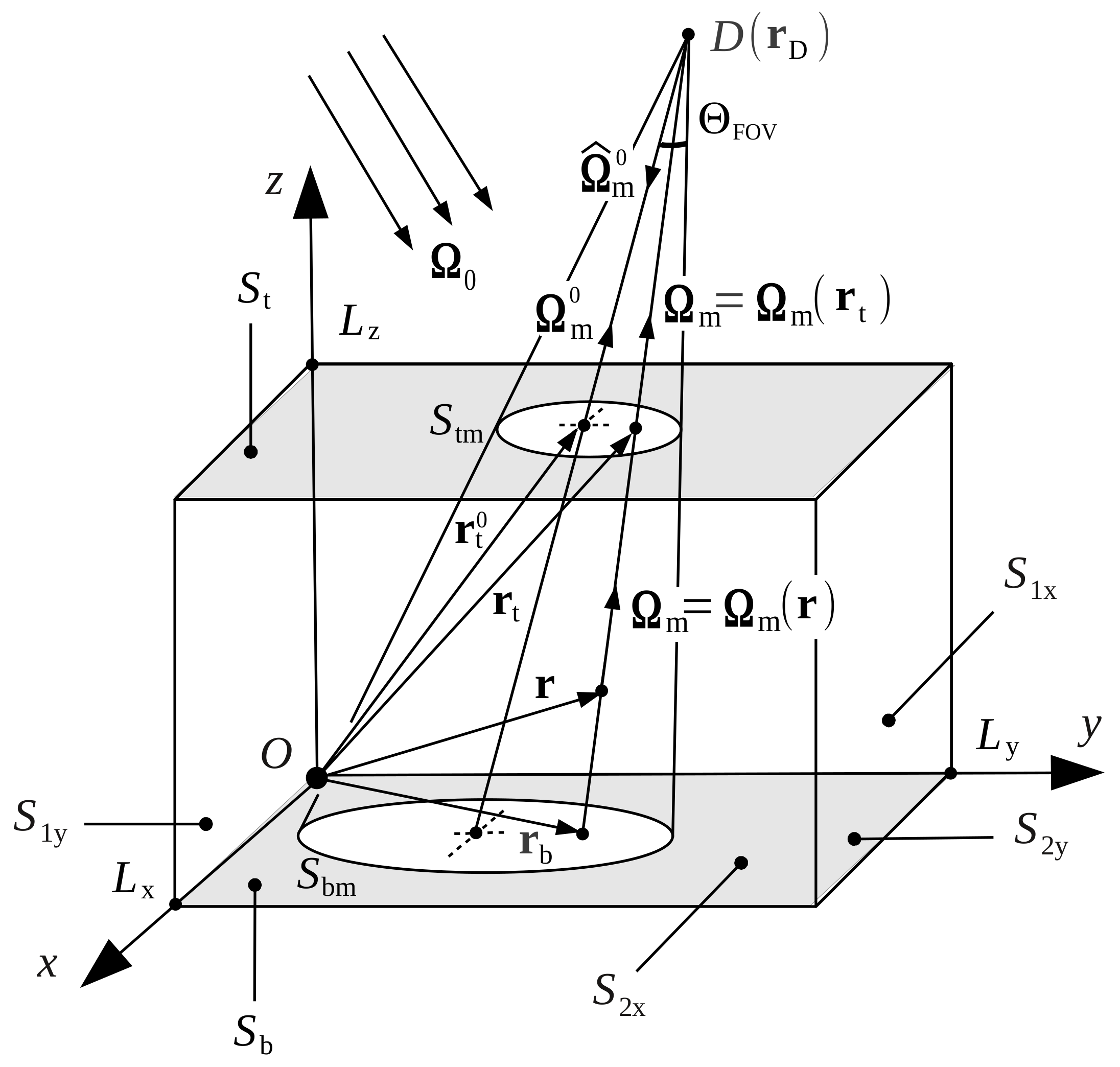
2. Problem Formulation

We consider the solar radiative transfer in a rectangular cuboid of lengths L x , L y and L z as shown in Figure 1. The top and the bottom faces of the prism are denoted by S t and S b , respectively, while the lateral faces are denoted by S 1 x ( x = 0 ), S 2 x ( x = L x ), S 1 y ( y = 0 ), and S 2 y ( y = L y ). The boundary-value problem for the total radiance at point r in direction Ω consists of the inhomogeneous differential equation (with the thermal emission term neglected)
d I d s ( r , Ω ) = σ ext ( r ) I ( r , Ω ) + σ sct ( r ) 4 π Ω P ( r , Ω , Ω ) I ( r , Ω ) d Ω ,
the top-of-atmosphere boundary condition
I ( r t , Ω ) = F 0 | μ 0 | δ ( Ω Ω 0 ) , r t S t ,
and the surface boundary condition
I ( r b , Ω + ) = 1 π Ω ρ ( r b , Ω + , Ω ) μ I ( r b , Ω ) d Ω , r b S b .
At the horizontal boundaries we assume periodic boundary conditions, i.e.,
I ( x = 0 , y , z , Ω ) = I ( x = L x , y , z , Ω ) , I ( x , y = 0 , z , Ω ) = I ( x , y = L y , z , Ω ) .
Here, σ ext and σ sct = ω σ ext are the extinction and scattering coefficients, respectively, ω is the single-scattering albedo, P is the phase function, ρ is the bidirectional surface reflection function, Ω 0 = ( μ 0 , φ 0 ) with μ 0 < 0 , is the solar direction, F 0 is the solar flux, Ω + and Ω denote an upward and a downward direction, respectively, Ω is the unit sphere, and Ω + and Ω stand for the upper and lower unit hemispheres, respectively.
Let us define the forward transport operator L by
L I ( r , Ω ) = d I d s ( r , Ω ) + σ ext ( r ) I ( r , Ω ) σ sct ( r ) 4 π Ω P ( r , Ω , Ω ) I ( r , Ω ) d Ω 1 π δ ( z ) H ( μ ) μ Ω ρ ( r , Ω , Ω ) H ( μ ) | μ | I ( r , Ω ) d Ω ,
and the forward source function Q ( r , Ω ) by
Q ( r , Ω ) = F 0 δ ( z L z ) δ ( Ω Ω 0 ) ,
where δ is the Dirac delta function and H is the Heaviside step function. It can be shown that if the radiation field I ( r , Ω ) solves the inhomogeneous operator equation
L I ( r , Ω ) = Q ( r , Ω ) ,
with the boundary conditions (4),
I ( r t , Ω ) = 0 , r t S t , and I ( r b , Ω + ) = 0 , r b S b ,
then I ( r , Ω ) solves the radiative transfer Equation (1) with the boundary conditions (2), (3), and (4). The converse result is also true.
The adjoint transport operator L is defined through the relation
L I , I = I , L I ,
where the scalar product of the fields I 1 and I 2 is given by
I 1 , I 2 = D Ω I 1 ( r , Ω ) I 2 ( r , Ω ) d Ω d V
and D is the domain of the rectangular cuboid. The expression of the adjoint operator, under the assumptions that (i) I satisfies the boundary conditions (4) and (8), and (ii) I satisfies the boundary conditions (4),
I ( r t , Ω + ) = 0 , r t S t , and I ( r b , Ω ) = 0 , r b S b ,
is given by
( L I ) ( r , Ω ) = d I d s ( r , Ω ) + σ ext ( r ) I ( r , Ω ) σ sct ( r ) 4 π Ω P ( r , Ω , Ω ) I ( r , Ω ) d Ω 1 π δ ( z ) H ( μ ) | μ | Ω ρ ( r , Ω , Ω ) H ( μ ) μ I ( r , Ω ) d Ω .
Note that the requirement of homogeneous and periodic boundary conditions for both I and I is essential when computing the adjoint of the differential operator d / d s by using the Gauss theorem over the domain D.
In our analysis we consider a situation which is typical for atmospheric remote sensing. Atmospheric radiation can be measured e.g., by a spectrometer, which in the following is called detector. The detector, which measures the radiance at the top of the atmosphere in the direction Ω m 0 = ( μ m 0 , φ m 0 ) , μ m 0 > 0 , is represented by a point with position vector r D = ( x D , y D , z D ) and is characterized by a characteristic function of its field of view χ FOV = χ FOV ( Ω m · Ω m 0 ) . The signal measured by the detector, can be written as
I = Ω χ FOV ( Ω m · Ω m 0 ) I ( r t ( Ω m ) , Ω m ) d Ω m ,
where I ( r t ( Ω m ) , Ω m ) is the radiance at the top of the atmosphere in direction Ω m . For the characteristic function χ FOV , we consider the representation
χ FOV ( Θ ) = 1 Ω FOV , 0 Θ Θ FOV 0 , otherwise ,
where Θ FOV and Ω FOV π Θ FOV 2 are the collecting polar and solid angles of the detector, respectively, and cos Θ = Ω m · Ω m 0 . Let S tm = S tm ( r D , Ω m 0 ) be the footprint of the detector on the top face S t , i.e., an ellipse centered at r t 0 = ( x t 0 , y t 0 , L z ) with the semi-major and semi-minor axes b = R D Θ FOV / μ m 0 and a = R D Θ FOV , respectively, where R D = | r D r t 0 | . Using the relation d Ω m = ( μ m 0 / R D 2 ) d S , where d S is the surface element on the top face S t , we express the measured signal as
I = S t h ( r t ) I ( r t , Ω m ( r t ) ) d S t ,
where
Ω m ( r t ) = r D r t | r D r t | = ( μ m ( r t ) , φ m ( r t ) ) ,
is the unit vector along the line connecting the points r t S tm and r D ,
h ( r t ) = 1 A tm , r t S tm 0 , otherwise
is the characteristic function associated to the detector footprint, and A tm = π a b = R D 2 Ω FOV / μ m 0 is the area of the ellipse.
The radiative transfer in an inhomogeneous three-dimensional medium is usually solved by a numerical method. Considering a spatial discretization of the domain of analysis, the extinction coefficient σ ext ( r ) , the single-scattering albedo ω ( r ), the Legendre expansion coefficients of the phase function χ n ( r ) (Appendix A), are specified at every grid point of the so-called base grid and trilinearly interpolated within each cell. Furthermore, the bidirectional surface reflection function ρ ( r b , Ω + , Ω ) is specified at every grid point on the bottom surface and in all upward and downward discrete ordinate directions.

3. Linearized SHDOM

In atmospheric remote sensing we are interested in the retrieval of say, N p atmospheric parameters ξ p , p = 1 , , N p , which determine the fields σ ext ( r ) , ω ( r ) , χ n ( r ) , and ρ ( r b , Ω + , Ω ) . The retrieval requires the knowledge of the weighting functions, i.e., the partial derivatives of the measured radiance with respect to the atmospheric parameters being retrieved, i.e., I / ξ p .

3.1. Linearized Forward Approach

The linearized forward approach relies on the analytical differentiation technique and is based on the fact that the radiance can be regarded as the composition of differentiable functions. By applying the chain rule repeatedly to these functions, derivatives of arbitrary order can be computed analytically. After choosing the independent variables with respect to which the derivatives of the radiance are required, the derivatives of each function are computed recursively, i.e., by repeatedly substituting the derivatives of the inner function in the chain rule.
The pertinent equations which are differentiated are given in Appendix A. Essentially, the analytical differentiation technique is applied to all steps of the algorithm including the transformation of the source function from spherical harmonics to discrete ordinates, the integration of the source function along discrete ordinate directions, the transformation of the discrete ordinate radiances to spherical harmonics, the calculation of the source function from the radiance in spherical harmonics space, the adaptive grid procedure, and the acceleration step. The benefit of this method is that no assumptions rather than those of the forward model have to be made. The disadvantage is that not only the radiance and the source function have to be stored at all grid points, but also their derivatives with respect to the atmospheric parameters of interest. As a result, the amount of required memory may exceed the size of RAM (several Gbytes).

3.2. Linearized Forward-Adjoint Approach

In view of Equation (15), the measured signal can be written as
I = Q , I ,
where
Q ( r , Ω ) = F 0 ( r t ) δ ( z L z ) δ ( Ω Ω m ( r ) ) ,
with
F 0 ( r t ) = h ( r t ) ,
is the adjoint source function. Here,
Ω m ( r ) = r D r | r D r | = ( μ m ( r ) , φ m ( r ) )
is the unit vector along the line joining the points r and r D , and r t = r + s Ω m ( r ) S tm with s = ( L z z ) / μ m ( r ) and r = ( x , y , z ) , is the intersection point of this line with the top face S t (Figure 1). Obviously, because the points r , r t , and r D are on the same line, we have Ω m ( r t ) = Ω m ( r ) , and so, μ m ( r t ) = μ m ( r ) .
The main result of the adjoint radiative transfer theory states that if (i) I solves the forward problem consisting in the operator equation L I = Q and the boundary conditions (4) and (8), and (ii) I solves the adjoint problem consisting in the operator equation L I = Q and the boundary conditions (4) and (11), then the measured signal I can be estimated either by the scalar product of the radiance field I (as determined by Q) and the adjoint source function Q , or by the scalar product of the adjoint radiance field I (as determined by Q ) and the forward source function Q, i.e.,
I = Q , I = L I , I = I , L I = I , Q .
The partial derivative of the measured signal with respect to some atmospheric parameter ξ p , can be computed as
I ξ p = Q , I ξ p = L I , I ξ p = I , L I ξ p ,
where in the first step we assumed that Q / ξ p = 0 , while in the last step we used the fact that I / ξ p satisfies the boundary conditions (4) and (8). Taking the partial derivative of the operator equation L I = Q with respect to ξ p and assuming Q / ξ p = 0 gives
I ξ p = I , L ξ p I .
It should be pointed out that in general, the linearized forward-adjoint approach can be used to compute the weighted integral of the partial derivative of the radiance field I / ξ p defined by
D p = Q , I ξ p .
In this case, employing the same arguments as in the derivation of Equations (23) and (24), but without assuming that Q / ξ p = 0 , we get
D p = I , L ξ p I .
Thus, identifying the adjoint source function from Equation (25) and solving the corresponding adjoint radiative transfer equation L I = Q , we can compute the weighted integral D p by means of Equation (26).
The forward and adjoint radiative transfer equations L I = Q and L I = Q , respectively, are related to each other. Replacing Ω by Ω in the expression of the adjoint operator L , gives L ( Ω ) I ( r , Ω ) = Q ( r , Ω ) . Defining the pseudo-forward field I ^ by the relation I ^ ( r , Ω ) = I ( r , Ω ) and using the symmetry properties of the phase function P ( r , Ω , Ω ) = P ( r , Ω , Ω ) and of the normalized reflection function ρ ( r b , Ω , Ω ) = ρ ( r b , Ω , Ω ) , we find the identity L ( Ω ) I ( r , Ω ) = L ( Ω ) I ^ ( r , Ω ) . Thus, the pseudo-forward field I ^ solves the same type of radiative transfer equation as the radiance field I, i.e., L I ^ = Q ^ , where the pseudo-forward source function, defined by Q ^ ( r , Ω ) = Q ( r , Ω ) , is
Q ^ ( r , Ω ) = F ^ 0 ( r t ) δ ( z L z ) δ ( Ω Ω ^ m ( r ) ) ,
with Ω ^ m ( r ) = Ω m ( r ) , μ ^ m ( r ) = μ m ( r ) , and
F ^ 0 ( r t ) = F 0 ( r t ) = h ( r t ) .
In other words, I ^ ( r , Ω ) solves the inhomogeneous differential equation
d I ^ d s ( r , Ω ) = σ ext ( r ) I ^ ( r , Ω ) + σ sct ( r ) 4 π Ω P ( r , Ω , Ω ) I ^ ( r , Ω ) d Ω
with the top-of-atmosphere boundary condition
I ^ ( r t , Ω ) = F ^ 0 ( r t ) | μ ^ m ( r t ) | δ ( Ω Ω ^ m ( r t ) ) , r t S t ,
and the surface boundary condition
I ^ ( r b , Ω + ) = 1 π Ω ρ ( r b , Ω + , Ω ) μ I ^ ( r b , Ω ) d Ω , r b S b .
We are now concern with the computation of the partial derivative I / ξ p by means of Equation (24). Taking the variation of the forward transport operator L under the assumption that the phase function does not depend on the atmospheric parameter ξ p , yields (cf. Equation (5))
( δ L I ) ( r , Ω ) = δ σ ext ( r ) I ( r , Ω ) δ σ ext ( r ) ω ( r ) 4 π Ω P ( r , Ω , Ω ) I ( r , Ω ) d Ω σ ext ( r ) δ ω ( r ) 4 π Ω P ( r , Ω , Ω ) I ( r , Ω ) d Ω 1 π δ ( z ) H ( μ ) μ Ω δ ρ ( r , Ω , Ω ) H ( μ ) | μ | I ( r , Ω ) d Ω .
In this section we describe the computation of the partial derivative of the measured signal with respect to a parameter that determine the extinction field; the partial derivatives with respect to parameters that specify the single-scattering albedo and the bidirectional reflection function are given in Appendix B.
To compute the partial derivatives of the forward operator we need to find appropriate interpolation schemes for the extinction coefficient, source function, and radiance field within a grid cell. A major problem arises from the fact that SHDOM uses the integral form of the radiative transfer equation for radiance calculation, and in particular, the assumption that the extinction/source function product varies linearly along the characteristic. Unfortunately, when dealing with the differential form of the radiative transfer equation, this assumption can not be met; instead, we may assume that the extinction/source function product varies linearly within a cell. Thus, different interpolation schemes are used for radiance and derivative calculations.
In the following, we assume that the partial derivatives σ ext ( r i ) / ξ p at all grid points r i are known. Let c be the global index of a cell containing a grid point with global index j, and let j ¯ be the local index of this point within cell c (Figure 2); we define the map g as ( j ¯ , c ) g j , or equivalently, j = g ( j ¯ , c ) . For r D c , where D c is the domain of cell c, we assume that the extinction and extinction/source function product vary linearly within the cell, i.e.
σ ext ( r ) = i ¯ L i ¯ ( R ) σ ext ( r g ( i ¯ , c ) )
and
σ ext ( r ) J ( r , Ω ) = i ¯ L i ¯ ( R ) σ ext ( r g ( i ¯ , c ) ) J ( r g ( i ¯ , c ) , Ω ) ,
respectively. Here,
J ( r , Ω ) = ω ( r ) 4 π Ω P ( r , Ω , Ω ) I ( r , Ω ) d Ω
is the source function, L i ¯ are the first-order interpolation basis functions for a rectangular cuboid element (Appendix C), R = r ρ c is the position vector of a point in a local coordinate system attached to cell c, ρ c = ( 1 / 8 ) i ¯ r g ( i ¯ , c ) is the position vector of the center point of cell c, r g ( i ¯ , c ) = r i is the position vector of the grid point with global index i = g ( i ¯ , c ) , and the sum i ¯ is taken over all grid points of a cell. Setting σ ext g ( i ¯ , c ) = σ ext ( r g ( i ¯ , c ) ) , we obtain
L ξ p I ( r , Ω ) = i ¯ L i ¯ ( R ) [ I ( r , Ω ) J ( r g ( i ¯ , c ) , Ω ) ] σ ext g ( i ¯ , c ) ξ p ,
implying
I ξ p = c i ¯ Ω D c L i ¯ ( R ) I ^ ( r , Ω ) [ I ( r , Ω ) J ( r g ( i ¯ , c ) , Ω ) ] σ ext g ( i ¯ , c ) ξ p d V d Ω .
In the next step, we split the total radiance I ( r , Ω ) into the diffuse and direct radiances, i.e.,
I ( r , Ω ) = I d ( r , Ω ) + δ ( Ω Ω 0 ) T 0 ( r ) ,
where
T 0 ( r ) = F 0 | μ 0 | e τ ext ( r , r 0 | Ω 0 )
is the transmission along the solar direction Ω 0 from the starting point r 0 = r s Ω 0 S t to the end point r (the forward direct beam), and
τ ext ( r , r 0 | Ω 0 ) = 0 s σ ext ( r 0 + s Ω 0 ) d s
is the optical depth. Similarly, we split the pseudo-forward radiance I ^ ( r , Ω ) into its diffuse and direct components, i.e.,
I ^ ( r , Ω ) = I ^ d ( r , Ω ) + δ ( Ω Ω ^ m ( r ) ) T ^ m ( r ) ,
where
T ^ m ( r ) = F ^ 0 ( r t ) | μ ^ m ( r t ) | e τ ext ( r , r t | Ω ^ m ( r ) ) ,
is the transmission along the detector direction Ω ^ m ( r ) from the starting point r t = r s Ω ^ m ( r ) S tm to the end point r (the pseudo-forward direct beam). Approximating
Ω m ( r ) = Ω ^ m ( r ) Ω m ( ρ c ) : = Ω m c , r D c ,
we are led to the following representation for I / ξ p in terms of diffuse radiances:
I ξ p = T A + T B + T C + T D + T E ,
where
T A = c i ¯ Ω D c L i ¯ ( R ) I ^ d ( r , Ω ) I d ( r , Ω ) σ ext g ( i ¯ , c ) ξ p d V d Ω ,
T B = c i ¯ Ω D c L i ¯ ( R ) I ^ d ( r , Ω ) J ( r g ( i ¯ , c ) , Ω ) σ ext g ( i ¯ , c ) ξ p d V d Ω ,
and
T C = c i ¯ D c L i ¯ ( R ) I ^ d ( r , Ω 0 ) T 0 ( r ) σ ext g ( i ¯ , c ) ξ p d V ,
T D = c i ¯ D c L i ¯ ( R ) T ^ m ( r ) I d ( r , Ω m c ) σ ext g ( i ¯ , c ) ξ p d V ,
T E = c i ¯ D c L i ¯ ( R ) T ^ m ( r ) J ( r g ( i ¯ , c ) , Ω m c ) σ ext g ( i ¯ , c ) ξ p d V .
The above integrals are computed in the spherical harmonics space by assuming the expansions
I d ( r , Ω ) = m n I m n ( r ) Y m n ( Ω ) ,
I ^ d ( r , Ω ) = m n I ^ m n ( r ) Y m n ( Ω ) ,
J ( r , Ω ) = m n J m n ( r ) Y m n ( Ω ) ,
where Y m n ( Ω ) are the orthonormal real-valued spherical harmonic functions (Appendix A), and the sum m n should be understood as
m n = m = M M n = | m | N ,
with N and M being the maximum expansion order and number of azimuthal modes, respectively. The linear approximation
f ( r ) = j ¯ L j ¯ ( R ) f ( r g ( j ¯ , c ) ) = j ¯ L j ¯ ( R ) f g ( j ¯ , c ) ,
where f ( r ) stands for I m n ( r ) , I ^ m n ( r ) , T 0 ( r ) , and T ^ m ( r ) , together with the identity Y m n ( Ω ) = ( 1 ) n Y m n ( Ω ) , then yield
T A = c m n ( 1 ) n i ¯ , j ¯ , k ¯ I ^ m n , g ( j ¯ , c ) I m n , g ( k ¯ , c ) σ ext g ( i ¯ , c ) ξ p L i ¯ , j ¯ , k ¯ ,
T B = c m n ( 1 ) n i ¯ , j ¯ I ^ m n , g ( j ¯ , c ) J m n , g ( i ¯ , c ) σ ext g ( i ¯ , c ) ξ p L i ¯ , j ¯ ,
and
T C = c i ¯ , j ¯ , k ¯ I ^ d ( r g ( j ¯ , c ) , Ω 0 ) T 0 g ( k ¯ , c ) σ ext g ( i ¯ , c ) ξ p L i ¯ , j ¯ , k ¯ ,
T D = c i ¯ , j ¯ , k ¯ I d ( r g ( j ¯ , c ) , Ω m c ) T ^ m g ( k ¯ , c ) σ ext g ( i ¯ , c ) ξ p L i ¯ , j ¯ , k ¯ ,
T E = c m n Y m n ( Ω m c ) i ¯ , j ¯ T ^ m g ( j ¯ , c ) J m n , g ( i ¯ , c ) σ ext g ( i ¯ , c ) ξ p L i ¯ , j ¯ .
Here, the interpolations coefficients L i ¯ , j ¯ , k ¯ and L i ¯ , j ¯ are given, respectively, by
L i ¯ , j ¯ , k ¯ = D c L i ¯ ( R ) L j ¯ ( R ) L k ¯ ( R ) d V ,
L i ¯ , j ¯ = D c L i ¯ ( R ) L j ¯ ( R ) d V ,
while for i = g ( i ¯ , c ) and ω i = ω ( r i ) , the expansion coefficients of the source function in Equations (55) and (58) are computed as
J m n , i = ω i χ n , i 2 n + 1 I m n , i + ω i χ n , i 2 n + 1 Y m n ( Ω 0 ) T 0 i ,
where χ n , i = χ n ( r i ) are the Legendre expansion coefficients of the phase function (Appendix A), i.e.,
P ( r , Ω , Ω ) = 4 π m n χ n ( r ) 2 n + 1 Y m n ( Ω ) Y m n ( Ω ) .
Further comments and algorithm details are given below:
1.
The input parameters of the numerical algorithm are the partial derivatives σ ext ( r i ) / ξ p and ω ( r i ) / ξ p at all grid points r i , and eventually, the partial derivatives ρ ( r b i , Ω i j + , Ω p q ) / ξ p at all grid points on the bottom surface r b i and in all upward and downward discrete ordinate directions Ω i j + and Ω p q , respectively.
2.
The interpolation coefficients L i ¯ , j ¯ , k ¯ and L i ¯ , j ¯ are computed analytically in a local coordinate system attached to the grid cell.
3.
The radiances I ^ d ( r g ( j ¯ , c ) , Ω 0 ) and I d ( r g ( j ¯ , c ) , Ω m c ) in the expressions of T C and T D , respectively, are computed by the source integration method.
4.
For solar problems with the delta-M method [24], the radiative transfer equation is expressed in terms of the scaled quantities
σ ¯ ext = ( 1 f ω ) σ ext , ω ¯ = 1 f 1 f ω ω ,
where f is the truncation fraction. At each grid point, we switch from the partial derivatives σ ext / ξ p and ω / ξ p to σ ¯ ext / ξ p and ω ¯ / ξ p , respectively, whereby the latter two are computed from Equation (63) by using the chain rule.
5.
The partial derivatives of the signal correction in the TMS method of Nakajima and Tanaka [25] are computed analytically (Appendix A).
6.
During the adaptive grid procedure, a base grid cell, also called a “parent cell”, is split into “child cells” to achieve higher spatial resolution. In this regard, the sums in Equations (54)–(58) are taken over all child cells.
7.
According to the main result of the adjoint radiative transfer theory, the measured signal can be computed by using Equation (15) or (22); in the latter case, the computational formula is
I = F 0 S t I ^ d ( x t , y t , L z , Ω 0 ) d S t .
8.
The code uses two alternative interpolation schemes for the source function: a linear variation of the extinction/source function product within a cell, i.e., Equation (34), and a linear variation of the source function within a cell, i.e.,
J ( r , Ω ) = i ¯ L i ¯ ( R ) J ( r g ( i ¯ , c ) , Ω ) ,
for r D c . In the second case, the terms T B and T E are computed, respectively, as
T B = c m n ( 1 ) n i ¯ , j ¯ , k ¯ I ^ m n , g ( j ¯ , c ) J m n , g ( k ¯ , c ) σ ext g ( i ¯ , c ) ξ p L i ¯ , j ¯ , k ¯ ,
T E = c m n Y m n ( Ω m c ) i ¯ , j ¯ , k ¯ T ^ m g ( j ¯ , c ) J m n , g ( k ¯ , c ) σ ext g ( i ¯ , c ) ξ p L i ¯ , j ¯ , k ¯ .
9.
In the case of satellite remote sensing we may assume that (i) the distance from the top of the atmosphere to the detector R D is sufficiently large, so that we can approximate I ( r , Ω m ( r ) ) I ( r , Ω m 0 ) , and (ii) the footprint of the detector is a rectangle of lengths 2 a and 2 b centered at r t 0 . The second assumption is made because the domain is discretized in rectangular cuboid elements. In this context, the measured signal is computed as
I = 1 4 a b S t h ¯ ( x t , y t ) I ( x t , y t , L z , Ω m 0 ) d S t ,
where the normalized characteristic function h ¯ ( x t , y t ) takes the value 1 inside the footprint of the detector and 0 otherwise.
10.
The solution of the adjoint problem is a challenging task due to the spatial discontinuity of the pseudo-forward direct beam. In SHDOM, this type of problem is handled by the adaptive grid procedure. Essentially, the adaptive grid supplies extra spatial resolution along the boundaries of the pseudo-forward direct beam, so that there are not large discontinuities in the grid. In order to reduce the number of adaptive grid cells, the step characteristic function of the detector can be replaced by a smooth function, e.g., trapezoidal, Gaussian, cosine [23]. In the first case, the normalized characteristic function reads as
h ¯ ( x t , y t ) = h ¯ 0 ( x t , Δ h x ) h ¯ 0 ( y t , Δ h y ) , ( x t , y t ) S tm 0 , otherwise ,
where, for example, h ¯ 0 ( x t , Δ h x ) is given by
h ¯ 0 ( x t , Δ h x ) = c x × x t x t min 0 Δ h x , x t min 0 x t < x t min 0 + Δ h x 1 , x t min 0 + Δ h x x t x t max 0 Δ h x x t max 0 x t Δ h x , x t max 0 Δ h x < x t x t max 0
with c x = 2 a / ( 2 a Δ h x ) , x t min 0 = x t 0 a , and x t max 0 = x t 0 + a .
11.
In the linearized forward-adjoint approach, the forward and adjoint problems are solved successively on the same grid; in this way, the interpolation between different grids is avoided. Actually, in the first step, the adjoint problem is solved by using the adaptive grid procedure with a prescribed splitting accuracy ε split (Appendix A), and in the second step, the forward problem is solved on the resulting grid without splitting. In the linearized forward approach, the forward problem is solved first by using the adaptive grid procedure, and then, the partial derivatives are computed on the same grid; in this way, a less amount of memory for storing the derivatives of the radiance and the source function with respect to the atmospheric parameters of interest is required.

4. Numerical Simulations
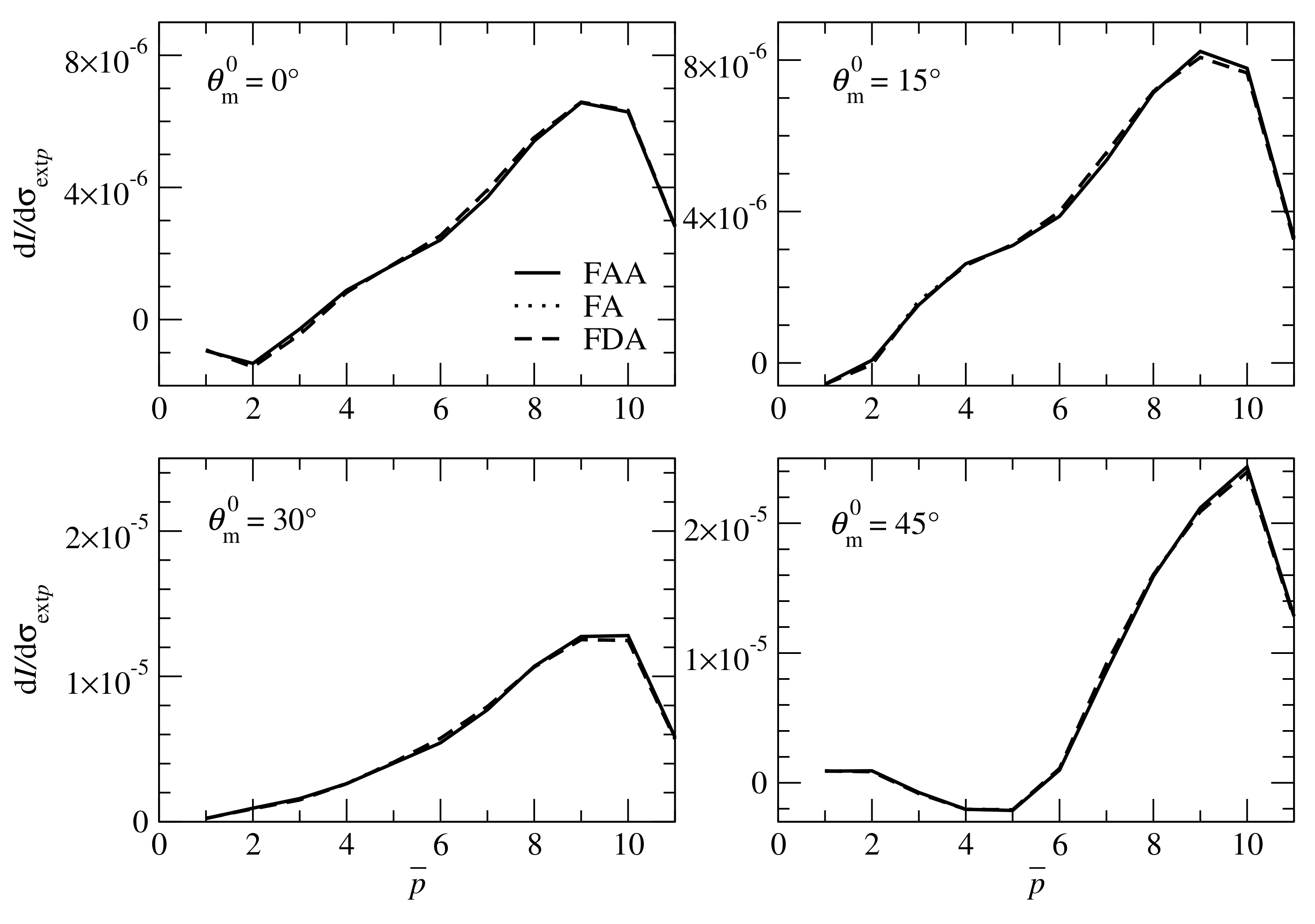
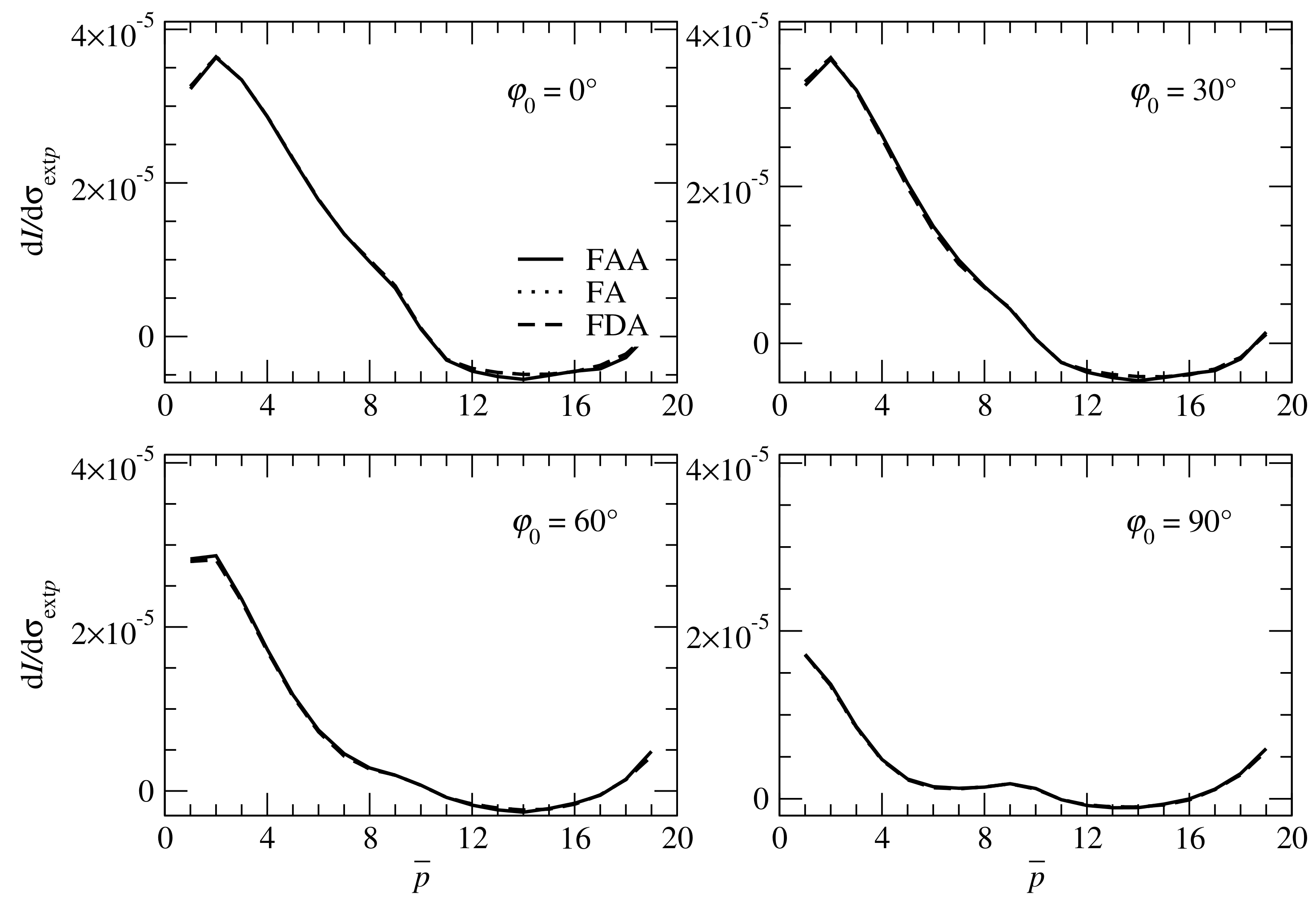
In this section we analyze the accuracy and efficiency of the linearized versions of SHDOM.

4.1. Example 1

We consider a base grid with N x = N y = 20 and N z = 11 points, and the discretization steps Δ x = Δ y = Δ z = 0.1 km. For periodic boundary conditions, when the vertical boundaries in x and y have additional planes of grid points that duplicate the grid points in the planes x = 0 and y = 0 , respectively, the domain of analysis has the sizes L x = N x Δ x = 2 km, L y = N y Δ y = 2 km, and L z = ( N z 1 ) Δ z = 1 km. The extinction field is Gaussian, i.e.,
σ ext ( x , y , z ) = σ ext max f ( x , y , z ) ,
f ( x , y , z ) = f G ( x , x 0 , s x ) f G ( y , y 0 , s y ) f G ( z , z 0 , s z ) ,
f G ( u , u 0 , s u ) = exp ( u u 0 ) 2 2 s u 2 , u = x , y , z ,
with x 0 = L x / 2 , y 0 = L y / 2 , z 0 = L z / 2 , s x = L x / 4 , s y = L y / 4 , and s z = L z / 4 . The parameters σ ext max is 6 km 1 , in which case, the peak optical depth is 3.6 . The extinction field in the plane y = L y / 2 is illustrated in Figure 3. The number of discrete zenith and azimuthal angles are N μ = 16 and N φ = 2 N μ , respectively, the single-scattering albedo is ω = 0.9 , and a Henyey–Greenstein phase function [26] with the asymmetry parameter g = 0.8 is considered. In all our simulations, the solar zenith angle is θ 0 = 120 , and a Lambertian reflecting surface with the surface albedo A = 0.2 is chosen. The coordinates of the center of the detector footprint are x t 0 = L x / 2 , y t 0 = L y / 2 , and z t 0 = L z , the detector azimuthal angle is φ m 0 = 0 , the lengths of the rectangular footprint are a = 5 Δ x , and b = [ a / ( Δ y μ m 0 ) ] Δ y , where [ x ] is the integer part of x, and the lengths specifying the slope of the characteristic function in Equation (70) are Δ h x = 0.5 Δ x and Δ h y = 0.5 Δ y .
In the following, we compute the partial derivatives of the measured signal with respect to the extinction coefficients σ ext p at N p = 11 base grid points ( x = x t 0 , y = y t 0 , z = p ¯ Δ z ), p ¯ = 1 , , N p . Obviously, if p is the global index of the grid point with the local index p ¯ in the derivative list, we have
σ ext i σ ext p = δ i p , ω i σ ext p = 0 .
First, we compare the accuracies of the measured signal and of its derivatives. The accuracy of SHDOM radiances is determined by the angular and spatial resolution, i.e., the number of discrete ordinates in zenith angle N μ and, for a specified base grid, the splitting accuracy ε split . In Figure 4, we plot the partial derivatives computed with the linearized forward-adjoint approach and the linearized approach for different values of the splitting accuracy ε split . Note that the influence of N μ on the results accuracy is rather low. Taking the values corresponding to ε split 0 = 5 × 10 4 as a reference, we illustrate in Table 1, the relative error in the partial derivatives, expressed as an rms difference normalized by the mean of the quantity over the N p comparison points, i.e.,
ε I = p ¯ I σ ext p ε split I σ ext p ε split 0 2 p ¯ I σ ext p ε split 0 2 ,
and the relative error in the measured signal, i.e.,
ε I = | I ε split I ε split 0 | / I ε split 0 .
The results show that for the same ε split ,
1.
the accuracy of the measured signal is higher than that of its derivatives, and
2.
the accuracy of the linearized forward-adjoint approach is higher than that of the linearized forward approach.
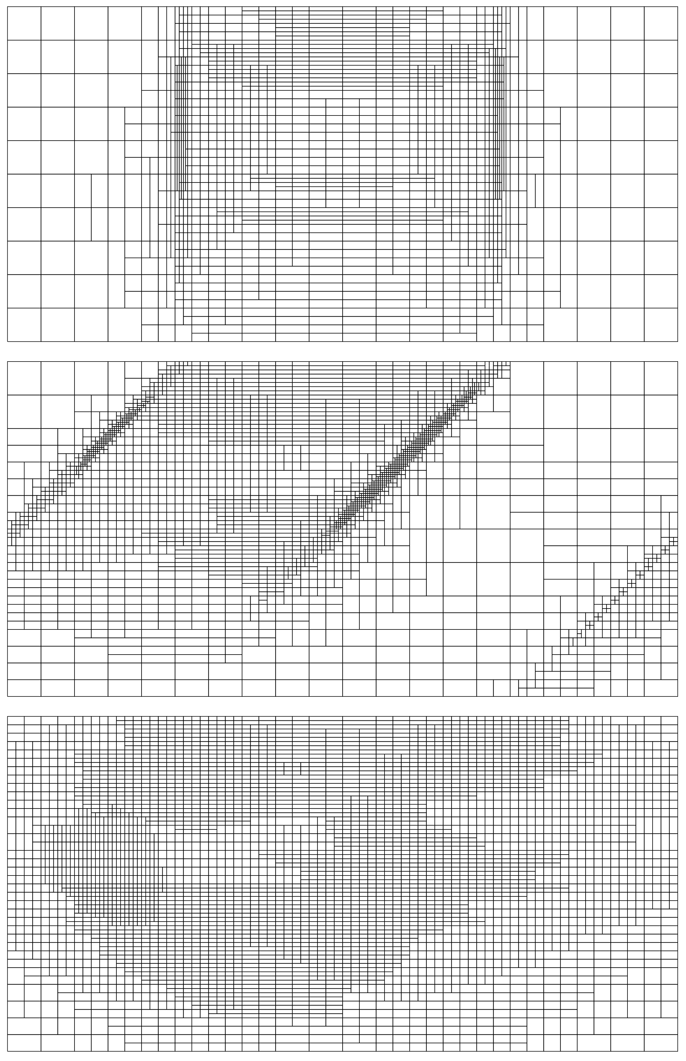
However, in the next calculations, to avoid a large CPU time and computer memory, we take ε split = 10 3 . For this splitting accuracy, we show in Figure 5, the adaptive grids in the plane y = L y / 2 . From these plots we infer that
1.
for the linearized forward-adjoint approach, the number of adaptive grid cells is higher in the domain “seen” by the detector along the direction θ m 0 and in particular, along the boundaries of the pseudo-forward direct beam,
2.
for the linearized forward approach, the number of adaptive grid cells is higher in the entire domain along the solar direction θ 0 = 120 and when large discontinuities in the source function are present, and
3.
in general, the number of adaptive grid cells for the linearized forward approach is grater than that for the linearized forward-adjoint approach.
In Figure 6 we plot the partial derivatives I / σ ext p for different values of the detector zenith angle θ m 0 . The results are computed with the linearized forward-adjoint approach (FAA), the linearized forward approach (FA), and the finite-difference approach (FDA). In the latter case, a centered finite difference scheme is used for derivative calculations. The partial derivatives I / σ ext p at N p = 19 base grid points ( x = p ¯ Δ x , y = y t 0 , z = L z / 2 ), p ¯ = 1 . , N p , for different values of the solar azimuthal angle φ 0 are plotted in Figure 7. Taking the values computed by the finite-difference approach as a reference, we illustrate in Table 2 the corresponding relative errors in the partial derivatives, defined, for example, in the case of the linearized forward-adjoint approach as
ε I FAA = p ¯ I σ ext p FAA I σ ext p FDA 2 p ¯ I σ ext p FDA 2 .
The relative errors corresponding to the linearized forward-adjoint approach are smaller than 2.5 × 10 2 , while the relative errors corresponding to the linearized forward approach are smaller than 4.3 × 10 3 . The relative large errors of the linearized forward-adjoint approach can be explained as follows.
.1
As it can be inferred from Figure 5, the linearized forward-adjoint approach uses a rougher discretization grid (depending on the detector zenith angle θ m 0 ) as compared to the forward and finite-difference approaches (which use the same grid).
2.
In the linearized forward-adjoint approach, the extinction/source function product is assumed to vary linearly within the cell, while in the forward and finite-difference approaches, the extinction/source function product is assumed to vary linearly along the characteristic.

4.2. Example 2

In the second example we consider in addition to the scattering and absorption by a cloud, molecular Rayleigh scattering, and the absorption by NO 2 at the wavelength λ = 443 nm. The difference to the previous geometry is that now we consider a base grid with N z = 16 points along the z axis, implying that the height of the domain of analysis is L z = ( N z 1 ) Δ z = 1.5 km. The cloud extinction field is given by Equations (71)–(73), while the cloud single-scattering albedo and the phase function are computed by Mie theory [27] for a water-cloud model with a Gamma size distribution
P a a α exp α a a mod
of parameters a eff = 10 μ m , a mod = 2 a eff / 3 , and α = 6 . Here, a is the particle radius, and the droplet size ranges between 0.02 and 50.0 μ m. The computed value for the cloud single-scattering albedo is ω cld = 0.865 , the Rayleigh cross-section and depolarization ratios are calculated as in [28], while the pressure and temperature profiles correspond to the US standard model atmosphere [29]. The number density and absorption cross section profiles for NO 2 , n ( z ) and C abs ( z ) , respectively, are shown in Figure 8, and the absorption coefficient is calculated as σ abs ( z ) = n ( z ) C abs ( z ) . The peak optical depth is 5.4 .
In the following, we compute the partial derivative of the measured signal with respect to maximum value of the extinction field σ ext max in Equation (71); in this case, we approximate P P cld and use
σ ext i σ ext max = f ( x i , y i , z i ) and ω i σ ext max = ω cld ω i σ ext i σ ext i σ ext max .
We also compute the partial derivative of the measured signal with respect to the total column of NO 2 , X = ( k B T 0 / p 0 ) 0 L z n ( z ) d z , where k B is the Boltzmann constant, and p 0 and T 0 are the standard pressure and temperature. Assuming that the number density profile for NO 2 is the a priori profile n a ( z ) scaled by a constant, i.e., n ( z ) = α n a ( z ) , where α is the scaling factor, we get
σ ext i X = 1 X a σ abs ( z i ) and ω i X = ω i σ ext i σ ext i X ,
implying σ sct i / X = 0 .
In Table 3 and Table 4, we illustrate the partial derivatives I / σ ext max and I / X , and the corresponding relative errors using the values computed by the finite-difference approach as a reference. Also shown are the relative errors of the measured signal computed by Equation (22) (or, equivalently, by Equation (64)) with respect to the measured signal computed by Equation (15). In these simulations, the number of discrete zenith angles is N μ = 20 , and the splitting accuracy is ε split = 3 × 10 3 . The relative errors corresponding to the linearized forward-adjoint approach are now smaller than 2.3 × 10 2 , while the relative errors corresponding to the linearized forward approach are smaller than 3.8 × 10 3 . It should be pointed out that the small errors in the measured signal certify that the adjoint problem is correctly solved.
In Table 5 we compare the computational efficiency of all linearization methods. Note that the code is parallelized with the OpenMP interface. The simulations are performed on a server Intel(R) Xeon(R) CPU E5-2695 v3 @ 2.30 GHz with 56 cores, while the CPU times are given for the parallelized implementation. Clearly, the most efficient method is the linearized forward-adjoint approach, while the most time-consuming method is the finite-difference approach.
Finally, in Table 6, we show the numbers of adaptive cells and grid points for the test problems considered in this study. Because in the linearized forward-adjoint approach, the numbers of cells and points are smaller than in the linearized forward approach, we infer that the first method is not only faster but also less memory demanding than the second one.

5. Conclusions

Two linearization methods for SHDOM have been discussed. The first method is an analytical linearization approach, while the second method is based on the adjoint radiative transfer theory. In the latter case, practical formulas for computing the derivatives of the measured signal in the spherical harmonics space have been derived. Essentially, SHDOM has been specialized for derivative calculations and radiative transfer problems involving the delta-M approximation, the TMS correction, and the adaptive grid splitting.
Our numerical analysis leads to the following conclusions.
1.
The linearized SHDOM with analytical derivatives is an accurate approach. However, the method is time-consuming and demands a large computer memory. The reason is that not only the source function has to be stored as a spherical harmonic series at each grid point, but also its derivatives with respect to the atmospheric parameters of interest.
2.
The linearized SHDOM with a forward-adjoint approach requires less storage for derivatives calculation, are much faster, but relatively less accurate. The main reason for this lower accuracy is that different interpolation schemes are used for radiance and derivative calculations.
According to our numerical analysis, the relative errors of the linearized forward-adjoint approach are smaller than 2.5%. In this regard, it should be pointed out that in the framework of the Gauss-Newton method, errors of about 2–3% in the Jacobian do not play a significant role. The effect is somehow similar to the computation of the root of an equation by the secant method instead of the Newton method. However, if the errors in the Jacobian are important for the retrieval, the regularized total least squares, which accounts on the errors in both the Jacobian and the data, can be used.
In our analysis, we considered the case of a fixed detector position r D and a single-angle measurement Ω m 0 . For multi-angle measurements and eventually, several detector positions, the solution of several adjoint problems (corresponding to each pair ( r D , Ω m 0 ) ) can be avoided by employing the approach proposed in Ref. [23]. The main ideas of this approach, which can be applied for multi-dimensional remote sensing of cloud extinction fields from airborne radiometer measurements, are discussed in Appendix D. However, it should be pointed out that the computational cost for the retrieval of 3D extinction fields is extremely high. A reduction of the computation time can be achieved if a two-dimensional geometry (a constant extinction field along the y-axis, and a set of directions on the unit sphere) is considered. In this case, the application of the forward-adjoint approach requires that both the solar and detector azimuthal angles are zero (the solar and detector directions are in the x z -plane).
Potential application of the linearized SHDOM include the following.
1.
Retrieval of cloud model parameters. For broken clouds [30], the indicator function f ( x , y , z ) in Equation (71) takes the values 1 inside the cloud and 0 inside the clear sky region. As in [31], the extinction field can be parametrized in terms of σ ext max (cf. Equation (71)), the cloud top height h t , and the cloud bottom height h b . The cloud optical thickness and the cloud geometrical parameters can be retrieved in the oxygen A-band by using the correlated k-distribution method for the broadband integration of the gaseous line absorption. Note that SHDOM is able to compute monochromatic and broadband radiative transfer (with a k distribution).
2.
Trace gas retrievals under cloudy conditions. The retrieval of total column of trace gases, e.g., O 3 , NO 2 , etc., can be performed by means of the differential optical absorption spectroscopy (DOAS) technique [32]. This approach requires the knowledge of the air mass factor (AMF), i.e., the partial derivative of the measured signal with respect to the total column of the trace gas at a specific wavelength. The main goal of the analysis is the computation of the air mass factor when clouds are outside the footprint of the instrument (effect of horizontal cloud edges on AMF calculation).

Author Contributions

Methodology, A.D.; Software, A.D. and D.S.E.; Writing—Original Draft Preparation, A.D. and D.S.E.; Writing—Review & Editing, A.D. and D.S.E.

Funding

This research received no external funding.

Acknowledgments

The authors are pleased to acknowledge very fruitful and stimulating discussions with Frank Evans during the completion of this work.

Conflicts of Interest

The authors declare no conflict of interest.

Appendix A

In this appendix we summarize the SHDOM algorithm in order to emphasize the main equations which are differentiated in the framework of the linearized forward approach.
SHDOM uses both spherical harmonics and discrete ordinates to represent the radiance field during different parts of the solution algorithm. The spherical harmonics are employed for computing the source function including the scattering integral, while the discrete ordinates are used to integrate the radiative transfer equation spatially.
The set of discrete ordinates are a reduced Gaussian grid. There are N μ Gaussian quadrature cosine zenith angles, μ j , and N φ evenly spaced azimuth angles, φ k . The discrete ordinate set is reduced by having fewer azimuth angles at larger | μ | j ; thus, N φ depends on j. The corresponding Gauss-Legendre quadrature weights and azimuthal integration weights (normalized appropriately) are w μ j and w φ j k , respectively.
The orthonormal real-value spherical harmonics are defined by
Y m n ( μ , φ ) = P n | m | ( μ ) u m ( φ ) ,
where P n | m | ( μ ) are the normalized associated Legendre functions, and
u m ( φ ) = ( 1 / π ) cos ( | m | φ ) ( 1 / 2 π ) ( 1 / π ) sin ( | m | φ ) m > 0 m = 0 m < 0
are the Fourier harmonics. The source function
J ( r , Ω ) = ω ( r ) 4 π Ω P ( r , Ω , Ω ) [ I d ( r , Ω ) + δ ( Ω Ω 0 ) T 0 ( r ) ] d Ω ,
T 0 ( r ) = F 0 | μ 0 | e τ ext ( r , r 0 | Ω 0 ) ,
where
τ ext ( r , r 0 | Ω 0 ) = 0 s σ ext ( r 0 + s Ω 0 ) d s
with s = | r r 0 |, is the optical depth from the point r to the upper domain boundary point r 0 along the solar direction Ω 0 , is expressed in the spherical harmonic space as
J ( r , Ω ) = m = M M n = | m | N J m n ( r ) Y m n ( Ω ) ,
where N = N μ 1 is the maximum expansion order and M = N φ / 2 1 is the maximum number of azimuthal modes.
By means of the addition theorem for the Legendre functions, the phase function, expanded in terms of unnormalized Legendre polynomials
P ˜ n ( cos Θ ) = 2 2 n + 1 P n ( cos Θ ) ,
as
P ( r , cos Θ ) = n = 1 N rank χ n ( r ) P ˜ n ( cos Θ ) ,
where χ n ( r ) are the Legendre phase function coefficients and N rank is the maximum expansion order of the phase function, is truncated in the spherical harmonic space as
P ( r , cos Θ ) = 4 π m = M M n = | m | N χ n ( r ) 2 n + 1 Y m n ( Ω ) Y m n ( Ω ) ,
where cos Θ = Ω · Ω .
The solution method is based on Picard iterations. At the beginning of each iteration step, the expansion coefficients J m n ( r i ) , m = M , M , n = | m | , N , are assumed to be known at all grid points r i . They are updated according to the following four computational steps.
 Step 1. 
The source function is transformed to discrete ordinates by means of the relation
J ( r i , μ j , φ k ) = m = M M u m ( φ k ) n = | m | N J m n ( r i ) P n | m | ( μ j ) .
 Step 2. 
The discrete ordinate radiance I d ( r i , μ j , φ k ) is computed from the source function J ( r i , μ j , φ k ) by integrating the radiative transfer equation. Essentially, (i) the radiances are computed at all grid points in all downward discrete ordinate directions by integrating the radiative transfer equation with the top boundary condition I d ( r t i , μ j , φ k ) = 0 , where ( μ j , φ μ j ) and ( w μ j , w φ j k ) are the quadrature nodes and weights in the lower hemisphere, (ii) the radiances at the bottom boundary grid points in all upward discrete ordinate directions ( μ j + , φ k + ) are computed from the boundary condition
I d ( r b i , μ j + , φ k + ) = 1 π ρ ( r b i , μ j + , φ k + , μ 0 , φ 0 ) μ 0 T 0 ( r b i ) + 1 π p = 1 N μ / 2 q = 1 N φ p w μ p w φ p q ρ ( r b i , μ j + , φ k + , μ p , φ q ) × | μ p | I d ( r b i , μ p , φ q ) ,
and (iii) the radiances are computed at all grid points in all upward discrete ordinate directions by integrating the radiative transfer equation with the boundary condition (A11).
 Step 3. 
The discrete ordinate radiance at each grid point is transformed to the spherical harmonic space according to
I m n ( r i ) = j = 1 N μ w μ j P n | m | ( μ j ) k = 1 N φ j w φ j k I d ( r i , μ j , φ k ) u m ( φ k ) .
 Step 4. 
At each grid point, the source function is computed from the radiance in the spherical harmonic space as
J m n ( r i ) = ω ( r i ) χ n ( r i ) 2 n + 1 I m n ( r i ) + ω ( r i ) χ n ( r i ) 2 n + 1 Y m n ( Ω 0 ) T 0 ( r i ) .
Some comments are in order.
1.
The radiance and source function are initialized before the solution iterations with an Eddington radiative transfer solution on independent columns of the base grid.
2.
The explicit form of the transforms in Equations (A10) and (A12) illustrates how the azimuthal and zenith angle parts partially separate. For more than about 12 azimuthal angles, an FFT is used for the azimuthal Fourier transform.
3.
In Step 2, the radiative transfer equation is integrated backward from each grid point to a grid cell face that has known radiances at its bounding grid points. In the short-characteristic method, the integration is across just one cell, while in the long characteristic method, the characteristic Ω j k = ( μ j , φ k ) is traced backward until the transmission falls below some minimum specified value. In the latter case, the error from interpolating the radiance at the grid cell face is reduced. According to the SHDOM difference scheme, the radiance at the exiting point A along a characteristic Ω j k , I d ( r A , Ω j k ) , is computed from the integral form of the radiative transfer equation
I d ( r A , Ω j k ) = I d ( r B , Ω j k ) e 0 s 0 σ ext ( r B + s Ω j k ) d s + S ( s 0 , J ) ,
where I d ( r B , Ω j k ) is the radiance at the entering point B, s 0 = | r A r B | is the distance between the points A and B, and
S ( s 0 , J ) = 0 s 0 σ ext ( r B + s Ω j k ) J ( r B + s Ω j k , Ω j k ) × e s s 0 σ ext ( r B + s Ω j k ) d s d s
is the integral of the source function along the characteristic. Setting σ ext A , B = σ ext ( r A , B ) and J A , B = J ( r A , B , Ω j k ) , and assuming that the extinction σ ext and the extinction/source function product σ ext J vary linearly along the characteristic, yields
S ( s 0 , J ) = 1 e τ ext 1 σ ext A + σ ext B [ σ ext A J A + σ ext B J B + σ ext A σ ext B 6 ( J A J B ) s 0 ] ,
for τ ext 2 , and
S ( s 0 , J ) = 1 e τ ext 1 σ ext A + σ ext B [ σ ext A J A + σ ext B J B + 2 σ ext A σ ext B σ ext A + σ ext B ( J A J B ) 1 2 τ ext + 2 e τ ext 1 e τ ext ] ,
for τ ext > 2 , where
τ ext = τ ext ( r A , r B | Ω j k ) = 0 s 0 σ ext ( r B + s Ω j k ) d s
is the optical depth along the characteristic. Note that under the above assumptions, the representation (A16) follows from an expansion of the solution to the first order in the path distance s 0 , while the representation (A17) is a particular case of the general solution derived in [33]. The exiting and the entering values of the extinction and extinction/source function product σ ext A , σ ext B , σ ext A J A , and σ ext B J B are computed by bilinear interpolation from the grid point values of the faces pierced by the characteristic, while the radiance is also bilinearly interpolated between the surrounding grid points to give the initial radiance I d ( r B , Ω j k ) for integration.
4.
To increase the convergence rate, an acceleration method based on geometrical convergence is applied. At the iteration step K, the “accelerated” source column vector is computed as
J acc ( K ) = J ( K ) + a Δ J ( K )
where J ( K ) is the column vector encapsulating the expansion coefficients J m n ( K ) ( r i ) , m = M , , M , n = | m | , , N , at all grid points r i , i.e., J ( K ) = [ J m n ( K ) ( r i ) ] ,
Δ J ( K ) = J ( K ) J ( K 1 ) ,
is the residual source vector at the iteration step K, and
a = 1 r cos ψ + r 1 + π / ( 2 ψ ) 1 + r 2 2 r cos ψ 1
with
r = | | Δ J ( N ) | | | | Δ J ( N 1 ) | | ,
cos ψ = ( Δ J ( N 1 ) ) T ( Δ J ( N ) ) | | Δ J ( N 1 ) | | | | Δ J ( N ) | | ,
is the acceleration parameter. The iterations are stopped when the solution criterion
| | Δ J ( N ) | | | | J ( N 1 ) | | ε sol
is satisfied, where ε sol is the solution tolerance.
5.
If the delta-M scaling method is applied, then the optical parameters σ ext , ω , and χ n are scaled before their use. The scaled quantities σ ¯ ext , ω ¯ , and χ ¯ n are given, respectively, by (the dependency on r is omitted)
σ ¯ ext = ( 1 f ω ) σ ext ,
ω ¯ = 1 f 1 f ω ω ,
χ ¯ n 2 n + 1 = 1 1 f χ n 2 n + 1 f , n = 0 , , N ,
where
f = 1 2 N + 3 χ N + 1
is the truncation fraction.
6.
The radiance at a specified direction Ω m and location r is computed by integrating the source function through the medium, while the spherical harmonic representation of the source function is transformed to the desired viewing direction Ω m .
7.
For solar problems with the delta-M method, the TMS method is used to compute the source function. This method replaces the scaled, truncated Legendre phase function expansion for the singly scattered solar radiation by the full, unscaled phase function expansion, while the multiply scattered contribution still comes from the truncated phase function. The source function at grid point r i in direction Ω m is then computed as
J ( r i , Ω m ) = m = M M n = | m | N J m n ( r i ) Y m n ( Ω m ) + Δ J ( r i , Ω m ) ,
Δ J ( r i , Ω m ) = F 0 | μ 0 | e τ ¯ ext ( r i , r i 0 | Ω 0 ) [ ω ¯ ( r i ) 1 f 1 4 π n = 1 N rank χ n ( r i ) P ˜ n ( cos Θ ) ω ¯ ( r i ) m = M M n = | m | N χ ¯ n ( r i ) 2 n + 1 Y m n ( Ω 0 ) Y m n ( Ω m ) ] ,
where cos Θ = Ω 0 · Ω m .
8.
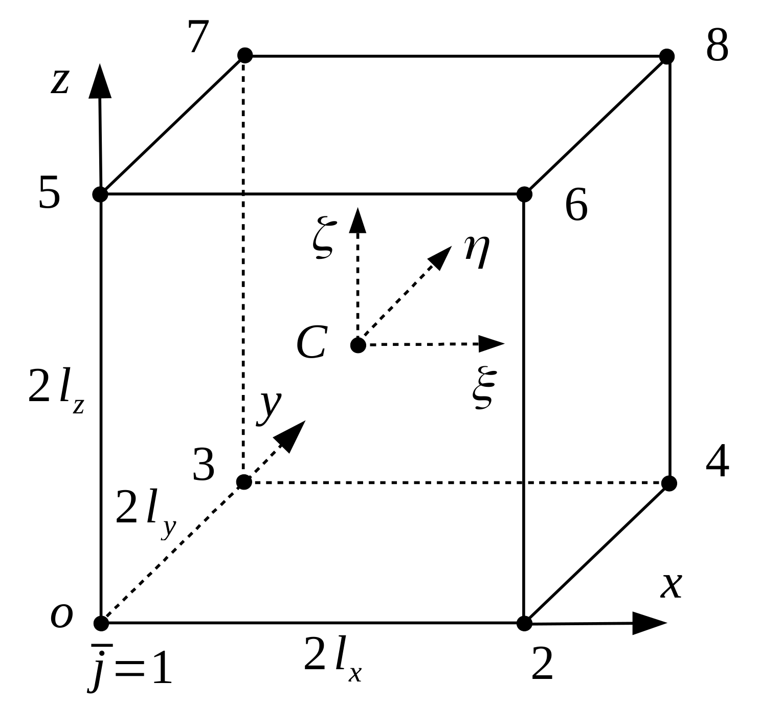
The adaptive grid evolves from the base grid by splitting cells where more resolution is judged to be needed. The criterion for splitting cells is based on how much the source function times extinction changes across a cell. A cell may be split in half in either of the three Cartesian directions, depending on whether any of them exceed the splitting criterion. For cell c, the cell-splitting criterion is
C c u j = | Δ J u j | ( 1 e τ u j ) ,
where u is one of the three Cartesian directions x, y, and z,
| Δ J u j | = 1 σ ¯ ext u j 1 4 π Ω [ σ ext u j + J ( r u j + , Ω ) σ ext u j J ( r u j . , Ω ) ] 2 d Ω = 1 σ ¯ ext u j 1 4 π m = M M n = | m | N [ σ ext u j + J m n ( r u j + ) σ ext u j J m n ( r u j ) ] 2 ,
r u j + F u + and r u j F u , j = 1 , 4 , are two cell corners along direction u, F u + and F u are the two cell faces crossed by direction u, τ u j = σ ¯ ext u j s u j , σ ¯ ext u j = ( σ ext u j + + σ ext u j ) / 2 , σ ext u j + = σ ext ( r u j + ) , σ ext u j = σ ext ( r u j ) , and s u j = | r u j + r u j | . The criterion is averaged over the four corners, i.e., C ¯ c u = ( 1 / 4 ) j = 1 4 C c u j , and the cells are sorted by the maximum over the splitting directions u = x , y , z of the averaged splitting criterion C ¯ c u . At the iteration step K, those cells c with the highest criterion C ¯ c u above a certain value ε split ( K ) are split first. The new cells may themselves be divided during one solution iteration. As the solution iterations proceed, the cell splitting accuracy ε split ( K ) is gradually lowered to the desired final cell-spliting accuracy ε split , and so more grid points are added at each iteration during this process.

Appendix B

The partial derivative of the measured signal with respect to a parameter ξ p that determine the single-scattering albedo at every grid point ω i = ω ( r i ) is computed in the spherical harmonic space as follows. For r D c , we assume that the extinction/source function product varies linearly within cell c, i.e.,
σ ext ( r ) J ( r , Ω ) = i ¯ = 1 L i ¯ ( R ) σ ext g ( i ¯ , c ) J ( r g ( i ¯ , c ) , Ω ) = i ¯ = 1 L i ¯ ( R ) σ ext g ( i ¯ , c ) ω g ( i ¯ , c ) 4 π Ω P ( r g ( i ¯ , c ) , Ω , Ω ) I ( r g ( i ¯ , c ) , Ω ) d Ω .
We obtain
L ξ p I ( r , Ω ) = i ¯ L i ¯ ( R ) [ σ ext g ( i ¯ , c ) 4 π × Ω P ( r g ( i ¯ , c ) , Ω , Ω ) I ( r g ( i ¯ , c ) , Ω ) d Ω ] ω g ( i ¯ , c ) ξ p ,
yielding
E ξ p = c i ¯ Ω D c L i ¯ ( R ) I ^ ( r , Ω ) [ σ ext g ( i ¯ , c ) 4 π × Ω P ( r g ( i ¯ , c ) , Ω , Ω ) I ( r g ( i ¯ , c ) , Ω ) d Ω ] ω g ( i ¯ , c ) ξ p d V d Ω .
Using
Ω P ( r , Ω , Ω ) I d ( r , Ω ) d Ω = 4 π m n χ n r 2 n + 1 I m n ( r ) Y m n ( Ω )
and
P ( r , Ω , Ω ) = 4 π m n χ n ( r ) 2 n + 1 Y m n ( Ω ) Y m n ( Ω ) ,
we end up with
I ξ p = T A + T B + T C + T D ,
where
T A = c m n ( 1 ) n i ¯ , j ¯ χ n , g ( i ¯ , c ) 2 n + 1 σ ext g ( i ¯ , c ) I m n , g ( i ¯ , c ) I ^ m n , g ( j ¯ , c ) ω g ( i ¯ , c ) ξ p L i ¯ , j ¯ ,
T B = c m n ( 1 ) n Y m n ( Ω 0 ) i ¯ , j ¯ χ n , g ( i ¯ , c ) 2 n + 1 σ ext g ( i ¯ , c ) T 0 g ( i ¯ , c ) I ^ m n , g ( j ¯ , c ) ω g ( i ¯ , c ) ξ p L i ¯ , j ¯ ,
and
T C = c m n Y m n ( Ω m c ) i ¯ , j ¯ χ n , g ( i ¯ , c ) 2 n + 1 σ ext g ( i ¯ , c ) I m n , g ( i ¯ , c ) T ^ m g ( j ¯ , c ) ω g ( i ¯ , c ) ξ p L i ¯ , j ¯ ,
T D = c m n Y m n ( Ω m c ) Y m n ( Ω 0 ) i ¯ , j ¯ χ n , g ( i ¯ , c ) 2 n + 1 σ ext g ( i ¯ , c ) T 0 g ( i ¯ , c ) T ^ m g ( j ¯ , c ) ω g ( i ¯ , c ) ξ p L i ¯ , j ¯ .
Considering the partial derivative of the measured signal with respect to a parameter ξ p that determine the bidirectional surface reflection function ρ ( r b , Ω + , Ω ) , we use Equation (32), to obtain
I ξ p = 1 π | μ 0 | μ m ( r b ) T 0 ( r b ) T ^ m ( r b ) ρ ξ p ( r b , Ω m ( r b ) , Ω 0 ) + 1 π | μ 0 | T 0 ( r b ) Ω H ( μ ) μ I ^ d ( r b , Ω ) ρ ξ p ( r b , Ω , Ω 0 ) d Ω + 1 π μ m ( r b ) T ^ m ( r b ) Ω ρ ξ p ( r b , Ω m ( r b ) , Ω ) × H ( μ ) | μ | I d ( r b , Ω ) d Ω + 1 π Ω H ( μ ) μ I ^ d ( r b , Ω ) × Ω ρ ξ p ( r b , Ω , Ω ) H ( μ ) | μ | I d ( r b , Ω ) d Ω d Ω .
The integrals over the unit sphere are computed in the discrete ordinate space under the assumption that the partial derivatives ρ / ξ p are known at all grid points on the bottom surface, and in all downward and upward discrete ordinate directions. For a Lambertian surface, ρ ( r b , Ω + , Ω ) is simply the albedo A, and for ξ p = A , the computational formula is
I A = 1 π | μ 0 | μ m ( r b i ) T 0 ( r b i ) T ^ m ( r b i ) + 1 π | μ 0 | T 0 ( r b i ) j = 1 N μ / 2 k = 1 N φ j w μ j w φ j k | μ j | I ^ d ( r b i , μ j , φ k ) + 1 π μ m ( r b i ) T ^ m ( r b i ) j = 1 N μ / 2 k = 1 N φ j w μ j w φ j k | μ j | I d ( r b i , μ j , φ k ) + 1 π j = 1 N μ / 2 k = 1 N φ j p = 1 N μ / 2 q = 1 N φ p w μ j w μ p w φ j k w φ p q | μ j | | μ p | × I ^ d ( r b i , μ j , φ k ) I d ( r b i , μ p , φ q ) .

Appendix C

Referring to Figure 2, the first-order interpolation basis functions for a rectangular cuboid element L i ¯ , i ¯ = 1 , 8 at a point r = ( x , y , z ) are given by
L 1 ( ξ , η , ς ) = n ( ξ ) n ( η ) n ( ς ) ,
L 2 ( ξ , η , ς ) = n + ( ξ ) n ( η ) n ( ς ) ,
L 3 ( ξ , η , ς ) = n ( ξ ) n + ( η ) n ( ς ) ,
L 4 ( ξ , η , ς ) = n + ( ξ ) n + ( η ) n ( ς ) ,
L 5 ( ξ , η , ς ) = n ( ξ ) n ( η ) n + ( ς ) ,
L 6 ( ξ , η , ς ) = n + ( ξ ) n ( η ) n + ( ς ) ,
L 7 ( ξ , η , ς ) = n ( ξ ) n + ( η ) n + ( ς ) ,
L 8 ( ξ , η , ς ) = n ( ξ ) n + ( η ) n + ( ς ) ,
where
n ± ( ξ ) = 1 2 ( 1 ± ξ )
are the one-dimensional linear interpolation functions, and ( ξ , η , ς ) are the normalized coordinates of the point in a local coordinate system attached to the center of the cell ρ c = ( x c , y c , z c ) , i.e.,
ξ = x x c l x , η = y y c l y , ς = z z c l z .

Appendix D

We consider the case of a detector with a fixed position r D , that measures the radiance in K directions Ω m k 0 , k = 1 , K . For the measurement direction Ω m k 0 , let S tm ( Ω m k 0 ) be the detector footprint centered at r t k 0 . We aim to compute the state vector ξ by minimizing the sum of squared residuals
R ( ξ ) = 1 2 k [ I ( ξ , Ω m k 0 ) I mes ( Ω m k 0 ) ] 2 ,
where I ( ξ , Ω m k 0 ) and I mes ( Ω m k 0 ) are the simulated and measured signals of the detector, respectively. In the steepest-descent method characterized by a linear convergence rate, the objective function is approximated by a linear model and the search direction is taken as the negative of the gradient g = R . By taking account of Equation (15), we deduce that the pth component of the gradient vector is given by
g p = R ξ p = k [ I ( ξ , Ω m k 0 ) I mes ( Ω m k 0 ) ] I ξ p ( ξ , Ω m k 0 ) = S t k [ I ( ξ , Ω m k 0 ) I mes ( Ω m k 0 ) ] × h k ( r t ) I ξ p ( r t , Ω m k 0 ) d S t ,
where
h k ( r t ) = 1 A tm k , r t S tm ( Ω m k 0 ) 0 , otherwise ,
A tm k = R D k 2 Ω FOV / μ m k 0 and R D k = | r D r t k 0 | . Further on, from Equation (25), we find that the adjoint source function reads as
Q ( r , Ω ) = k F 0 k ( r t ) δ ( z L z ) δ ( Ω Ω m k 0 ) ,
where
F 0 k ( r t ) = [ I ( ξ , Ω m k 0 ) I mes ( Ω m k 0 ) ] h k ( r t ) .
Thus, in each inversion step, we first solve the forward problem and compute the residual I ( ξ , Ω m k 0 ) I mes ( Ω m k 0 ) , and then solve the adjoint problem with the adjoint source function (A58) and compute each component of the gradient of the residual function g p by means of Equation (26). In this approach, the pseudo-forward direct beam is a superposition of direct beams corresponding to each Ω m k 0 . Consequently, if the angular domain covered by the measurements is large, it may happens that the spatial discontinuity of the pseudo-forward direct beam is not present.

References

  1. Ingmann, P.; Veihelmann, B.; Langen, J.; Lamarre, D.; Stark, H.; Bazalgette Courrèges-Lacoste, G. Requirements for the GMES Atmosphere Service and ESA’s implementation concept: Sentinels-4/-5 and -5p. Remote Sens. Environ. Sentin. Missions Oppor. Sci. 2012, 120, 58–69. [Google Scholar] [CrossRef]
  2. Kokhanovsky, A. The influence of horizontal inhomogeneity on radiative characteristics of clouds: An asymptotic case study. IEEE Trans. Geosci. Remote Sens. 2003, 41, 817–825. [Google Scholar] [CrossRef]
  3. Marshak, A.; Platnick, S.; Várnai, T.; Wen, G.; Cahalan, R.F. Impact of three-dimensional radiative effects on satellite retrievals of cloud droplet sizes. J. Geophys. Res. 2006, 111. [Google Scholar] [CrossRef]
  4. Efremenko, D.S.; Schüssler, O.; Doicu, A.; Loyola, D. A stochastic cloud model for cloud and ozone retrievals from UV measurements. J. Quant. Spectrosc. Radiat. Transf. 2016, 184, 167–179. [Google Scholar] [CrossRef]
  5. Zhuravleva, T.B.; Nasrtdinov, I.M.; Russkova, T.V. Influence of 3D cloud effects on spatial-angular characteristics of the reflected solar radiation field. Atmos. Ocean. Opt. 2017, 30, 103–110. [Google Scholar] [CrossRef]
  6. Efremenko, D.S.; Doicu, A.; Loyola, D.; Trautmann, T. Fast Stochastic Radiative Transfer Models for Trace Gas and Cloud Property Retrievals Under Cloudy Conditions. In Springer Series in Light Scattering; Springer International Publishing: Basel, Switzerland, 2018; pp. 231–277. [Google Scholar]
  7. Evans, K. The spherical harmonic discrete ordinate method for three-dimensional atmospheric radiative transfer. J. Atmos. Sci. 1998, 55, 429–446. [Google Scholar] [CrossRef]
  8. Pincus, R.; Evans, K. Computational cost and accuracy in calculating three-dimensional radiative transfer: Results for new implementations of Monte Carlo and SHDOM. J. Atmos. Sci. 2009, 66, 3131–3146. [Google Scholar] [CrossRef]
  9. Spherical Harmonic Discrete Ordinate Method (SHDOM) for Atmospheric Radiative Transfer. Available online: http://coloradolinux.com/shdom/ (accessed on 20 April 2019).
  10. Doicu, A.; Efremenko, D.; Trautmann, T. A multi-dimensional vector spherical harmonics discrete ordinate method for atmospheric radiative transfer. J. Quant. Spectrosc. Radiat. Transf. 2013, 118, 121–131. [Google Scholar] [CrossRef]
  11. Emde, C.; Barlakas, V.; Cornet, C.; Evans, F.; Korkin, S.; Ota, Y.; Labonnote, L.C.; Lyapustin, A.; Macke, A.; Mayer, B.; et al. IPRT polarized radiative transfer model intercomparison project—Phase A. J. Quant. Spectrosc. Radiat. Transf. 2015, 164, 8–36. [Google Scholar] [CrossRef]
  12. Spurr, R.; Kurosu, T.; Chance, K. A linearized discrete ordinate radiative transfer model for atmospheric remote-sensing retrieval. J. Quant. Spectrosc. Radiat. Transf. 2001, 68, 689–735. [Google Scholar] [CrossRef]
  13. Spurr, R. LIDORT and VLIDORT. Linearized pseudo-spherical scalar and vector discrete ordinate radiative transfer models for use in remote sensing retrieval problems. In Light Scattering Reviews; Kokhanovsky, A., Ed.; Springer: Berlin/Heidelberg, Germany, 2008; Volume 3, pp. 229–275. [Google Scholar]
  14. Marchuk, G. Equation for the value of information from weather satellite and formulation of inverse problems. Cosm. Res. 1964, 2, 394–409. [Google Scholar]
  15. Marchuk, G.I. Adjoint Equations and Analysis of Complex Systems; Springer: Cham, Switzerland, 1995. [Google Scholar]
  16. Landgraf, J.; Hasekamp, O.; Box, M.; Trautmann, T. A linearized radiative transfer model for ozone profile retrieval using the analytical forward-adjoint perturbation theory approach. J. Geophys. Res. Atmos. 2001, 106, 27291–27305. [Google Scholar] [CrossRef] [Green Version]
  17. Ustinov, E.A. Adjoint sensitivity analysis of radiative transfer equation: Temperature and gas mixing ratio weighting functions for remote sensing of scattering atmospheres in thermal IR. J. Quant. Spectrosc. Radiat. Transf. 2001, 68, 195–211. [Google Scholar] [CrossRef]
  18. Box, M. Radiative perturbation theory: A review. Env. Model. Softw. 2002, 17, 95–106. [Google Scholar] [CrossRef]
  19. Walter, H.; Landgraf, J.; Hasekamp, O. Linearization of a pseudo-spherical vector radiative transfer model. J. Quant. Spectrosc. Radiat. Transf. 2004, 85, 251–283. [Google Scholar] [CrossRef]
  20. Ustinov, E. Atmospheric weighting functions and surface partial derivatives for remote sensing of scattering planetary atmospheres in thermal spectral region: General adjoint approach. J. Quant. Spectrosc. Radiat. Transf. 2005, 92, 351–371. [Google Scholar] [CrossRef]
  21. Rozanov, V.; Rozanov, A. Relationship between different approaches to derive weighting functions related to atmospheric remote sensing problems. J. Quant. Spectrosc. Radiat. Transf. 2007, 105, 217–242. [Google Scholar] [CrossRef]
  22. Martin, W.; Cairns, B.; Bal, G. Adjoint methods for adjusting three-dimensional atmosphere and surface properties to fit multi-angle/multi-pixel polarimetric measurements. J. Quant. Spectrosc. Radiat. Transf. 2014, 144, 68–85. [Google Scholar] [CrossRef] [Green Version]
  23. Martin, W.G.; Hasekamp, O.P. A demonstration of adjoint methods for multi-dimensional remote sensing of the atmosphere and surface. J. Quant. Spectrosc. Radiat. Transf. 2018, 204, 215–231. [Google Scholar] [CrossRef]
  24. Wiscombe, W. The delta-M method: Rapid yet accurate radiative flux calculations for strongly asymmetric phase functions. J. Atmos. Sci. 1977, 34, 1408–1422. [Google Scholar] [CrossRef]
  25. Nakajima, T.; Tanaka, M. Algorithms for radiative intensity calculations in moderately thick atmos using a truncation approximation. J. Quant. Spectrosc. Radiat. Transf. 1988, 40, 51–69. [Google Scholar] [CrossRef]
  26. Henyey, L.C.; Greenstein, J.L. Diffuse radiation in the Galaxy. Astrophys. J. 1941, 93, 70. [Google Scholar] [CrossRef]
  27. Mie, G. Beitraege zur Optik trueber Medien, speziell kolloidaler Metalloesungen. Ann. Phys. 1908, 330, 377–445. [Google Scholar] [CrossRef]
  28. Bodhaine, B.A.; Wood, N.B.; Dutton, E.G.; Slusser, J.R. On rayleigh optical depth calculations. J. Atmos. Ocean. Technol. 1999, 16, 1854–1861. [Google Scholar] [CrossRef]
  29. Anderson, G.; Clough, S.; Kneizys, F.; Chetwynd, J.; Shettle, E. AFGL Atmospheric Constituent Profiles (0–120 km); AFGL-TR-86-0110; Air Force Geophysics Laboratory: Hanscom Air Force Base, MA, USA, 1986.
  30. Alexandrov, M.; Marshak, A.; Ackerman, A. Cellular Statistical Models of Broken Cloud Fields. Part I: Theory. J. Atmos. Sci. 2010, 67, 2125–2151. [Google Scholar] [CrossRef]
  31. García, V.M.; Sasi, S.; Efremenko, D.S.; Doicu, A.; Loyola, D. Linearized radiative transfer models for retrieval of cloud parameters from EPIC/DSCOVR measurements. J. Quant. Spectrosc. Radiat. Transf. 2018, 213, 241–251. [Google Scholar] [CrossRef] [Green Version]
  32. Platt, U.; Stutz, J. Differential Optical Absorption Spectroscopy: Principles and Applications; Springer: Berlin/Heidelberg, Germany, 2008. [Google Scholar]
  33. Doicu, A.; Efremenko, D.; Trautmann, T. An analysis of the short-characteristic method for the spherical harmonic discrete ordinate method (SHDOM). J. Quant. Spectrosc. Radiat. Transf. 2013, 119, 114–127. [Google Scholar] [CrossRef]
Figure 1. Illustration of the radiative transfer problem.
Atmosphere 10 00292 g001
Figure 2. Rectangular cuboid element with lengths 2 l x , 2 l y , and 2 l z . C is the center point of the cell, and j ¯ = 1 , , 8 is the local index of a grid point.
Atmosphere 10 00292 g002
Figure 3. Extinction field in the plane y = L y / 2 .
Atmosphere 10 00292 g003
Figure 4. Partial derivatives I / σ ext p at the base grid points ( x = x t 0 , y = y t 0 , z = p ¯ Δ z ), p ¯ = 1 , , 11 , computed with the linearized forward-adjoint approach (upper panel) and the linearized forward approach (lower panel) for different values of the splitting accuracy ε split . The detector zenith angle is θ m 0 = 0 , and the solar azimuthal angle is φ 0 = 0 .
Atmosphere 10 00292 g004
Figure 5. Adaptive grids in the plane y = L y / 2 corresponding to the linearized forward-adjoint approach with θ m 0 = 0 (upper panel) and θ m 0 = 45 (middle panel), and the linearized forward approach (lower panel). The solar azimuthal angle is φ 0 = 0 . The horizontal axis is the x-axis, while the vertical axis is the z-axis.
Atmosphere 10 00292 g005
Figure 6. Partial derivatives I / σ ext p at the base grid points ( x = x t 0 , y = y t 0 , z = p ¯ Δ z ), p ¯ = 1 , , 11 , for different values of the detector zenith angle θ m 0 . The results correspond to the solar azimuthal angle φ 0 = 0 and are computed with the linearized forward-adjoint approach (FAA), the linearized forward approach (FA), and the finite-difference approach (FDA).
Atmosphere 10 00292 g006
Figure 7. Partial derivatives I / σ ext p at the base grid points ( x = p ¯ Δ x , y = y t 0 , z = L z / 2 ), p ¯ = 1 , , 19 , for different values of the solar azimuthal angle φ 0 . The results correspond to the detector zenith angle θ m 0 = 45 and are computed with the linearized forward-adjoint approach (FAA), the linearized forward approach (FA), and the finite-difference approach (FDA).
Atmosphere 10 00292 g007
Figure 8. Number density (left) and absorption cross section (right) profiles for NO 2 .
Atmosphere 10 00292 g008
Table 1. Relative errors ε I and ε I for different values of the splitting accuracy ε split . The results correspond to the linearized forward-adjoint approach (FAA) and the linearized forward approach (FA).
ε split FAAFA
ε I ε I ε I ε I
8 × 10 4 1.06 × 10 2 1.16 × 10 4 3.00 × 10 2 8.70 × 10 5
1 × 10 3 1.42 × 10 2 1.49 × 10 4 3.83 × 10 2 2.07 × 10 4
3 × 10 3 4.22 × 10 2 8.36 × 10 4 6.22 × 10 2 7.05 × 10 4
5 × 10 3 5.58 × 10 2 1.04 × 10 3 7.75 × 10 2 1.42 × 10 3
Table 2. The first part of the table shows the relative errors ε I in the partial derivatives I / σ ext p at the base grid points ( x = x t 0 , y = y t 0 , z = p ¯ Δ z ), p ¯ = 1 , , 11 , for different values of the detector zenith angle θ m 0 , while the second part shows the relative errors ε I in the partial derivatives I / σ ext p at the base grid points ( x = p ¯ Δ x , y = y t 0 , z = L z / 2 ), p ¯ = 1 , , 19 , for different values of the solar azimuthal angle φ 0 . The results are computed with the linearized forward-adjoint approach (FAA) and the linearized forward approach (FA).
θ m 0 φ 0 ε I
FAA FA
0 ° 0 ° 2.50 × 10 2 4.02 × 10 3
15 ° 0 ° 2.23 × 10 2 4.28 × 10 3
30 ° 0 ° 2.42 × 10 2 3.22 × 10 3
45 ° 0 ° 2.05 × 10 2 1.29 × 10 3
45 ° 0 ° 7.35 × 10 3 9.74 × 10 4
45 ° 30 ° 1.64 × 10 2 6.52 × 10 4
45 ° 60 ° 1.56 × 10 2 3.97 × 10 4
45 ° 90 ° 1.21 × 10 2 3.10 × 10 3
Table 3. Partial derivative I / σ ext max , and the relative errors ε I and ε I for different values of the detector zenith angle θ m 0 . The results correspond to the solar azimuthal angle φ 0 = 0 and are computed with the linearized forward-adjoint approach (FAA) and the linearized forward approach (FA).
θ m 0 I / σ ext max ε I ε I
FAAFA
0 5.776 × 10 4 4.20 × 10 4 3.46 × 10 3 2.03 × 10 3
15 1.439 × 10 3 5.53 × 10 4 4.86 × 10 3 2.76 × 10 4
30 2.930 × 10 3 2.30 × 10 5 3.40 × 10 3 2.53 × 10 4
45 5.499 × 10 3 8.19 × 10 5 1.81 × 10 3 1.52 × 10 4
Table 4. Partial derivative I / X , and the relative errors ε I and ε I for different values of the detector zenith angle θ m 0 . The results correspond to the solar azimuthal angle φ 0 = 0 ° and are computed with the linearized forward-adjoint approach (FAA) and the linearized forward approach (FA).
θ m 0 I / X ε I ε I
FAAFA
0 ° 1.184 × 10 3 4.20 × 10 4 1.65 × 10 2 3.42 × 10 3
15 ° 1.284 × 10 3 5.53 × 10 4 2.27 × 10 2 3.70 × 10 3
30 ° 1.428 × 10 3 2.30 × 10 5 2.26 × 10 2 2.82 × 10 3
45 ° 2.529 × 10 3 8.19 × 10 5 2.20 × 10 2 3.06 × 10 3
Table 5. CPU time in min:sec for the test problems considered in this study and corresponding to the linearized forward-adjoint approach (FAA), the linearized forward approach (FA), and the finite-difference approach (FDA). The detector zenith angle is θ m 0 = 45 ° and the solar azimuthal angle is φ 0 = 0 ° .
Partial Derivatives FAA FA FDA
I / σ ext p (Figure 6)1:1627:12138:19
I / σ ext p (Figure 7)1:4732:34153:26
I / σ ext max 0:322:212:24
I / X 0:312:202:20
Table 6. The first part of the table shows the number of adaptive cells N cells and the final number of grid points N points for computing the derivatives I / σ ext p with the splitting accuracy ε split = 10 3 , while the second part of the table shows N cells and N points for computing the derivatives I / σ ext max and I / X with the splitting accuracy ε split = 3 × 10 3 . The results correspond to the linearized forward-adjoint approach (FAA) and the linearized forward approach (FA).
ε split θ m 0 FAAFA
N cells N points N cells N points
10 3 0 ° 66,652 40,727 293,492 162,279
10 3 15 ° 81,174 50,381 293,492 162,279
10 3 30 ° 95,152 59,595 293,492 162,279
10 3 45 ° 115,186 73,332 293,492 162,279
3 × 10 3 0 ° 17,804 13,196 54,164 33,576
3 × 10 3 15 ° 20,094 14,942 54,164 33,576
3 × 10 3 30 ° 22,674 16,989 54,164 33,576
3 × 10 3 45 ° 25,806 19,607 54,164 33,576

