1. Introduction
The measurement of
rotational temperatures is used as a proxy for atmospheric temperatures near the mesopause, but significant problems exist in their measurement. von Savigny et al. [
1] demonstrated that the altitude of peak
emission varied with vibrational level, and Cosby and Slanger [
2], Noll et al. [
3], and Hart [
4] all showed that measured
rotational temperatures were strongly dependent upon the upper vibrational level. Pendleton et al. [
5], Cosby and Slanger [
2], and Noll et al. [
3] all found significant deviations from local thermal equilibrium (LTE) for the higher
rotational levels, which artificially increase measured rotational temperatures. The Einstein
A coefficients are another source of uncertainty in the measurement of
rotational temperatures, and numerous researchers, such as Mies [
6], Langhoff et al. [
7], Turnbull and Lowe [
8], Goldman et al. [
9], Cosby and Slanger [
2], and Liu et al. [
10], have attempted to identify the transition probabilities which best reflect observations.
Mies [
6] used the theoretical dipole moment of Stevens et al. [
11] to derive transition probabilities, and in a comparison with available data found discrepancies in prior rotational temperature measurements. Langhoff et al. [
7] also used a theoretical electronic dipole moment function (EDMF) to derive the transition probabilities for the electronic ground state of the
molecule. By comparing the average ratio of Einstein
A coefficients, Langhoff et al. [
7] determined that their theoretical transition probabilities better matched observations than the transition probabilities of Mies [
6].
Turnbull and Lowe [
8] used an empirical EDMF to calculate the electronic ground state transition probabilities of the
molecule. To test the validity of their transition probabilities, they calculated the population of a single vibrational level using multiple overtones as this technique should yield the same population for all overtones. Turnbull and Lowe [
8] found the transition probabilities of Mies [
6] and Langhoff et al. [
7] both failed this test, and determined that their transition probabilities derived consistent populations for a single upper vibrational level using multiple overtones.
Nelson et al. [
12] used the relative intensities of 88 pairs of transitions of the
electronic ground state to measure the
dipole moment. These relative intensities provided detailed information about the shape of the
EDMF, and the transition probabilities. Goldman et al. [
9] used the improved line positions of Abrams et al. [
13] and Melen et al. [
14], along with the EDMFs of Nelson et al. [
12] and Chackerian et al. [
15], to determine the electronic ground state
line parameters for a larger range of rotational states. van der Loo and Groenenboom [
16] derived a new EDMF for
in the ground electronic state based upon high-level ab initio calculations. They primarily found good agreement with the EDMF of Nelson [
12], except at large atomic separations, where the EDMF of Nelson [
12] decreased too fast. Using their EDMF, van der Loo and Groenenboom [
16] calculated new transition probabilities for the
molecule.
Cosby and Slanger [
2] employed the method of Turnbull and Lowe [
8] to find the transition probabilities that best matched the sky spectra collected by astronomical instruments, and found the transition probabilities of Goldman et al. [
9] best matched their observations. Liu et al. [
10] calculated the
,
,
,
, and
rotational temperatures using the transition probabilities from Mies [
6], Turnbull and Lowe [
8], Rothman et al. [
17], van der Loo and Groenenboom [
16], and Langhoff [
7]. These rotational temperatures were compared to the Sounding of the Atmosphere using Broadband Emission Radiometry (SABER) volume emission rate (VER) profile weighted temperatures to determine which set of Einstein
A coefficients best matched the observations. Liu et al. [
10] determined that the coefficients of Langhoff [
7] were the most consistent with the SABER data.
In this paper, we use the large number of sky spectra in the Apache Point Observatory Galactic Evolution Experiment (APOGEE) dataset to examine the effect that the Einstein
A coefficients have upon ground-based
rotational temperature measurements. The Einstein
A coefficients used in this paper were taken from Mies [
6], Turnbull and Lowe [
8], Rothman et al. [
17], van der Loo and Groenenboom [
16], and Langhoff [
7]. Column density calculations were also made using the five sets of Einstein
A coefficients, and the effect they have upon column density measurements was examined. The APOGEE measured
rotational temperatures were compared to the simultaneous SABER satellite-based observations, in an attempt to determine which set of Einstein
A coefficients best reflected physical conditions. Both APOGEE and SABER observe emission from the
transition minimizing systematic errors due to the stratification of the
vibrational levels, and were observed concurrently to minimize seasonal differences. Four of the five sets of Einstein
A coefficients tested yielded nearly identical mean rotational temperatures, but the Einstein
A coefficients were found to have a significant impact upon the measured
vibrational populations.
This manuscript is divided into eight sections. The introduction concludes here in
Section 1.
Section 2 details the data sets and data reduction methods used in this work. In
Section 3 the fundamentals of
airglow emission are examined, and in
Section 4 the emission lines used in this work are optimized. In
Section 5 the Einstein
A coefficients used in this work are listed, and their resultant measured rotational temperatures and populations are detailed. Next, in
Section 6 the measured rotational temperatures are compared to SABER VER weighted temperatures, and in
Section 7 the results of this work are compared with previous measurements. Finally, in
Section 8, the manuscript concludes with a summary of the results from this analysis.
2. Data
Multiple datasets were used in this analysis. Ground-based observations were acquired from the APOGEE dataset, and night-time space-based observations from SABER, coincident with the ground-based observing site, were also gathered. The observations used in this study span over 2 years, and the complimentary observations allow for a deeper investigation into the effects that the Einstein A coefficients have upon ground-based rotational temperature measurements.
2.1. APOGEE
The Sloan Digital Sky Survey (SDSS) APOGEE instrument uses the SDSS dedicated 2.5 m
/5 modified Ritchey–Chretien telescope. The SDSS telescope has a
diameter field of view with each fiber sub-tending 2 arcseconds in diameter on the sky, and is located at the Apache Point Observatory (APO), Sunspot, New Mexico, USA, latitude 32.78
longitude −105.82
, at an elevation of 2788 m. The APOGEE spectrograph operates from 1.51 to 1.7
m with a resolution of approximately
/
≈ 22,500. For more detailed information on the APOGEE spectrograph and its performance, see Wilson et al. [
18] or Wilson et al. [
19], and for more information on the APOGEE data reduction pipeline, see Nidever et al. [
20]. The APOGEE spectrograph is fiber fed by 300 fibers, and typically 35 of the 300 fibers are dedicated to astronomically blank patches of sky which are termed sky fibers. The APOGEE sky spectra are collected for the intended purpose of removing the background atmospheric airglow emission present in astrophysical science spectra during the data reduction process. The APOGEE sky spectra used in this work represent over 4200 observations, totaling nearly 150,000 spectra, taken between June 15, 2011 and June 23, 2013 with each having a 500 second integration time. The APOGEE spectra contain the
and
ro-vibrational transitions from the
first overtone. In this work we only examined the
transition as it matches the emission sampled by the SABER instrument.
Astronomical spectra are acquired through a range of zenith angles, thus line intensities
are normalized to a zenith observation
using the van Rhijn [
21] conversion
where
h is the height of the emitting layer, assumed to be approximately 87 km, and
R is the radius of the Earth. APOGEE spectra are in units of erg/sec/Å/cm
which for the further use in intensity calculations were converted to units of Rayleighs per Å. Rayleighs have the dimensions of
photons/sec/cm
, and when divided by the corresponding Einstein
A coefficient, provide a direct measure of the column density of a species responsible for an emission process at a given wavelength. Rees et al. [
22] found that horizontal wind velocities near the mesopause could exceed 100 m/s, and on average were 10 m/s. A single APOGEE spectrum of 500 s integration time would on average sample a volume of air 5 km in length, assuming an average 10 m s
horizontal wind velocity. The entire field of view of the SDSS telescope is approximately 5 km in diameter at the height of the mesopause, consequently the APOGEE sky spectra in a single observation are effectively sampling overlapping volumes of atmosphere.
2.2. SABER
The Thermosphere Ionosphere Mesosphere Energetics and Dynamics (TIMED) satellite was launched in December of 2001, and has been continuously monitoring the Earth’s atmosphere since. The SABER instrument on board the TIMED satellite performs limb scan measurements of the Earth’s atmosphere creating temperature, pressure, density, and VER profiles. In this work SABER data version 1.07 was used, and for a more detailed treatment of the SABER instrument see Russell et al. [
23].
SABER measures atmospheric limb emission in 10 broadband radiometer channels ranging from 1.27 to 17
m, and atmospheric temperature profiles with a 2 km height resolution are derived from 15
m
emission measurements. The uncertainties in the SABER
temperature profiles vary from 1% at 80 km, 2% at 88 km, to over 20% at 110 km, and Garcia-Comas et al. [
24] determined that the largest single error in the temperature measurements was due to the uncertainty in the quenching rate of
by atomic oxygen. Additional information on SABER’s kinetic temperature measurements using
emission can be found in Mertens et al. [
25] or Mertens et al. [
26].
The SABER channel B measures the
VER around 1.6
m which is composed of the
and
ro-vibrational transitions. Noll et al. [
3] found an approximately 1 K difference between rotational temperatures measured from the
and
transitions with the
transition being warmer. In the work by Noll et al. [
27], they found an effective upper vibrational level
for the SABER channel B, implying that it effectively measured an average VER of the 2 transitions.
All night-time SABER observations that began within a 50 km radius of APO were obtained. The atmospheric profiles from SABER are not measured in a strict vertical sense, but instead ranges nearly 3° in latitude. The largest variations in atmospheric profiles occur in a latitudinal sense, and the SABER measurements used in this work are intended to measure average atmospheric characteristics at a comparable geographic latitude to APO. The SABER observations of APO totaled over 8800 observations from 2001 to 2015. SABER has made approximately 75 observations which occurred during an APOGEE observation, and in these 75 observations there are approximately 2600 spectra.
2.3. Measurement Errors
The APOGEE survey is designed to measure chemical abundances and radial velocities, and unfortunately flux standards are not observed. Consequently, the APOGEE spectra are not flux calibrated in a typical manner. To allow for better sky subtraction, APOGEE corrects for fiber-to-fiber throughput variations which are on the order of 10%. After the throughput variations are corrected, Nidever et al. [
20] reports that the flux variations in the
emission lines are less than 5% over a single observation. Using the histogram of the ratio of two flats taken two years apart, Nidever et al. [
20] found the one
spread of the distribution to be 0.002, which they primarily attribute to photon statistics, showing that the response of the APOGEE instrument is extremely stable over time. After fiber-to-fiber variations are corrected each spectrum is scaled by a wavelength dependent spectral response function to apply an approximate relative flux calibration.
The lack of flux calibration for the APOGEE data would at first appear to be problematic, but this work was focused on measuring line temperatures which are more dependent upon relative flux levels of the lines in a single spectrum rather than an absolute flux scale. The measurement of column densities should also not be significantly impacted as it is measured in the rotational temperature calculation process rather than from absolute flux levels.
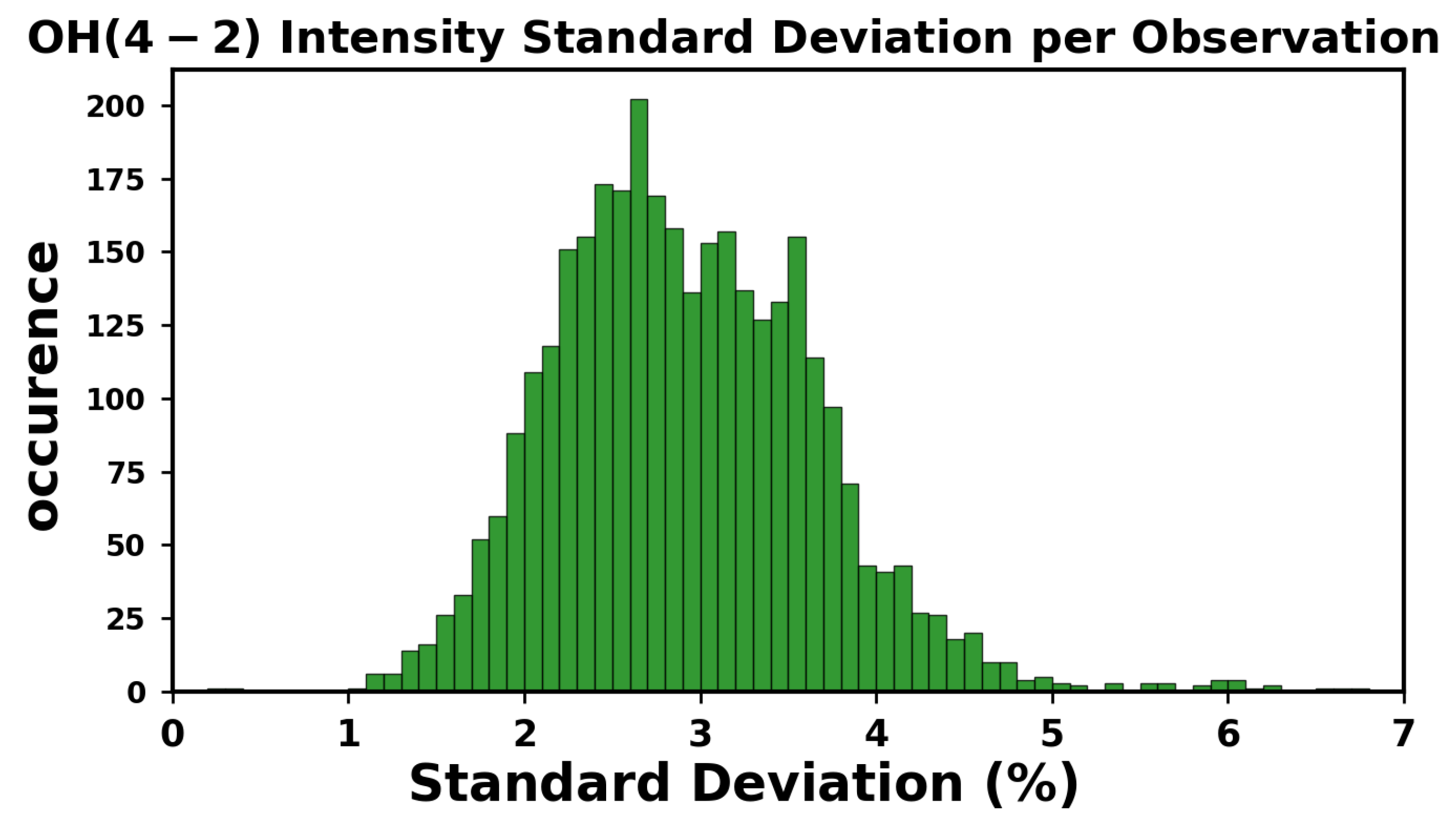
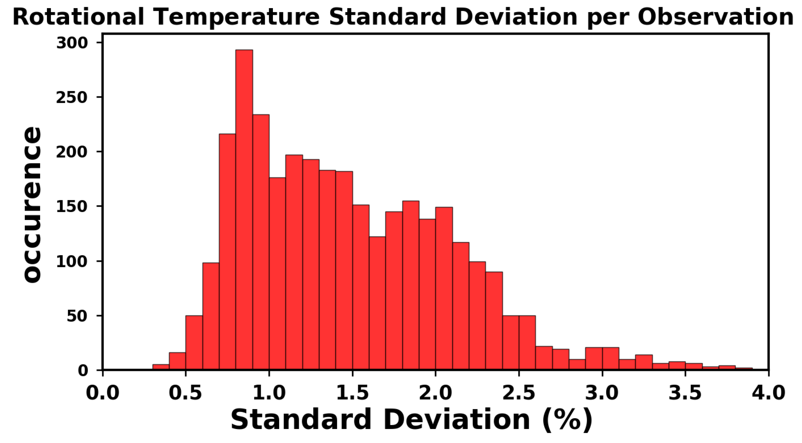
Fiber-to-fiber variations in a single observation are comprised of instrumental throughput differences, gradients in airglow intensity across the field of view, data reduction errors, and shot noise. In the measurement of the emission intensity the standard deviation per observation, the standard deviation of all the fibers from a single pointing, was less than 5%. The largest errors in the line measurements in this work are due to errors in the measurement and subtraction of the continuum, and contamination of lines by an adjacent emission line. The standard deviation per observation for all lines considered in this work was less than 1%, and for the measurement of rotational temperature the standard deviation per observation was at most 3%. The one flux variations over the entire APOGEE dataset used in this work were approximately 40% which is roughly equivalent in magnitude to the nightly and annual variations in emission intensity.
Although the standard deviation of an observation does not give any measure of absolute error, it is a measure of instrumental and data reduction errors. Distributions of the standard deviation per observation for the
intensity is shown in
Figure A1 and can be found in
Appendix A. The distribution of standard deviation per observation of the
rotational temperatures has also been included for reference in
Figure A2. In both
Figure A1 and
Figure A2, the observation standard deviations have been normalized by their respective observation mean to give the variation in terms of a percentage.
3. OH Emission
Bates and Nicolet [
28] found that the
molecule is primarily created by the ozone hydration reaction
which occurs around an altitude of 87 km, near the mesopause, in a narrow layer of approximately 10 km in height. Charters et al. [
29], Llewellyn et al. [
30], and Ohoyama et al. [
31] found that the reaction in Equation (
2) produces
molecules in the 9
th, 8
th, and 7
th vibrational states. Vibrational relaxation of the
molecule are due to radiative transitions and collisional relaxation.
Each vibrational level of the
molecule is accompanied by a range of rotational states. Radiative vibrational relaxations are typically accompanied by a change in rotational angular momentum termed ro-vibrational transitions. The selection rules for the rotational transitions are
, giving rise to
Q,
P, and
R branches. The
R branch transitions correspond to
with
, where
is the final rotational state and
is the initial. The
Q branch transitions correspond to
, and the
P branch transitions correspond to
.
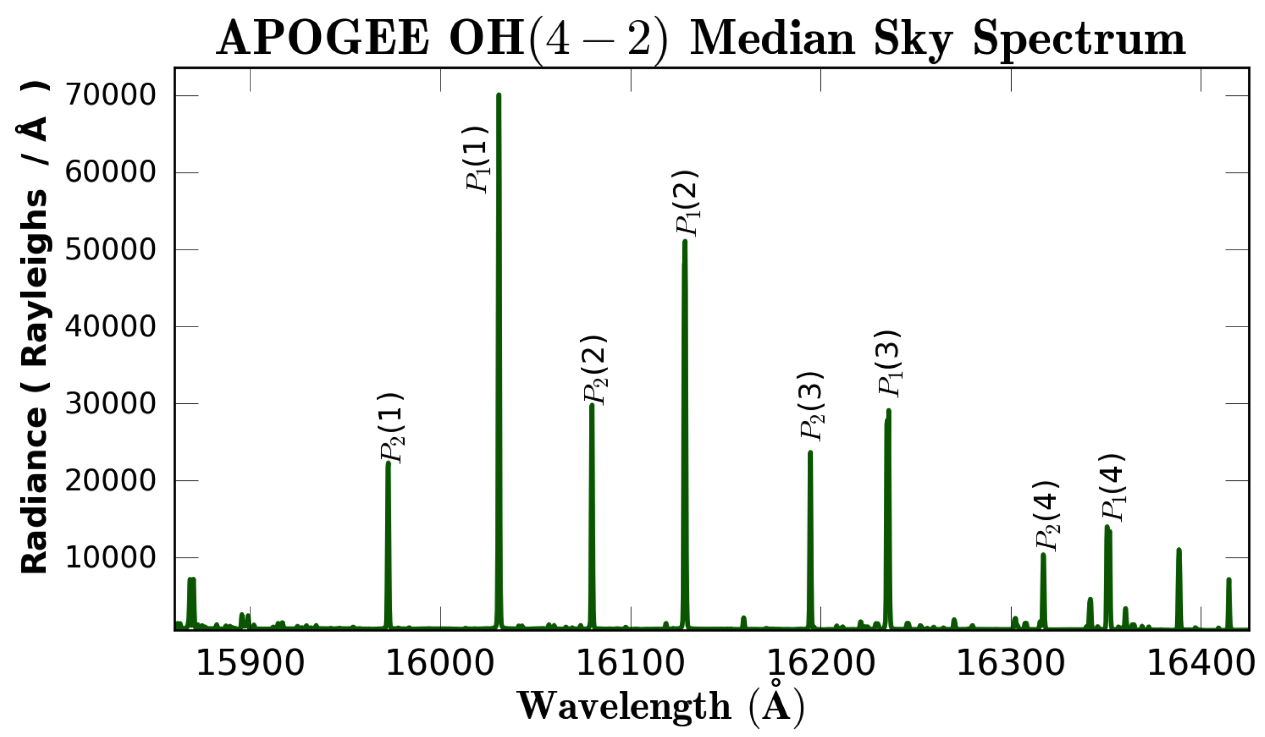
Figure 1 is the median APOGEE
spectrum with emission lines from the
P branch labeled.
emission in the optical and infrared is from the ground electronic state, and is composed of two sub-states. This multiplet structure, referred to as spin-splitting, is an effect that occurs due to the interaction between the electron spin vector and the projection of the orbital angular momentum vector along the internuclear axis. The transitions correspond to the electronic sub-state , which have a total of 3/2 electron spin and orbital angular momentum projected onto the internuclear axis. Whereas the transitions correspond to the electronic sub-state , which have a projected total angular momentum of 1/2. The ground electronic state of the molecule is inverted as the energy levels of the states are lower than the energy levels of the states, and the emission lines of the transitions are brighter than the emission lines of the transitions. Although some molecules do make transitions from the to the state, and vice versa, these transitions are rare and too faint to be observed in the APOGEE spectra.
The value in parenthesis in
Figure 1 is the rotational quantum number of the upper state. A common notation used in molecular spectroscopy uses
, where
represents the lowest final total angular momentum state for the branch. In the case for
the total final angular momentum is
, and for
the total final angular momentum is
.
The coupling of rotational motion further splits the
and
sub-states.
doubling splits each energy level into
and
components. The APOGEE spectra are of sufficient resolution to begin resolving some of the
doublets with a resolution element having a width of 0.6 Å at 1.5
m. Osterbrock et al. [
32], in their line atlas, only list
doublets with spacings greater than 0.2 Å, and Rousselot et al. [
33], in their line atlas, use a 1 Å threshold. Due to the rotational coupling nature of the
doublets, the spacing of the doublets increases with increasing angular momentum. In
Figure 1 the
and
emission lines both have resolved
doublets each with a spacing in excess of 1 Å.
OH Rotational Temperature
For an
vibrational level in thermal equilibrium with the surrounding atmosphere, the populations of the lower rotational states are well described by an isothermal Boltzmann distribution
where
is the population of the lowest rotational state of the vibrational level
,
is the electronic degeneracy, the
term represents the degeneracy of the rotational states,
k is the Boltzmann constant,
is the rotational term value of the upper state in units of cm
, and
T is the rotational temperature in Kelvins. The column density of the
state is given by
where
is the measured intensity of the
transition in Rayleighs,
is the Einstein
A coefficient for the particular transition in units of s
,
is the initial vibrational and rotational state, and
is the final state. Rotational temperatures are determined by measuring the slope of a linear fit to
versus
as similarly performed by Cosby and Slanger [
2] and Noll et al. [
3]. The population of the lowest rotational level,
, is derived from the intercept of the rotational fit, and to accomplish this the energy of the
emission line is shifted to zero energy. Lastly, the other emission lines are shifted by the same amount.
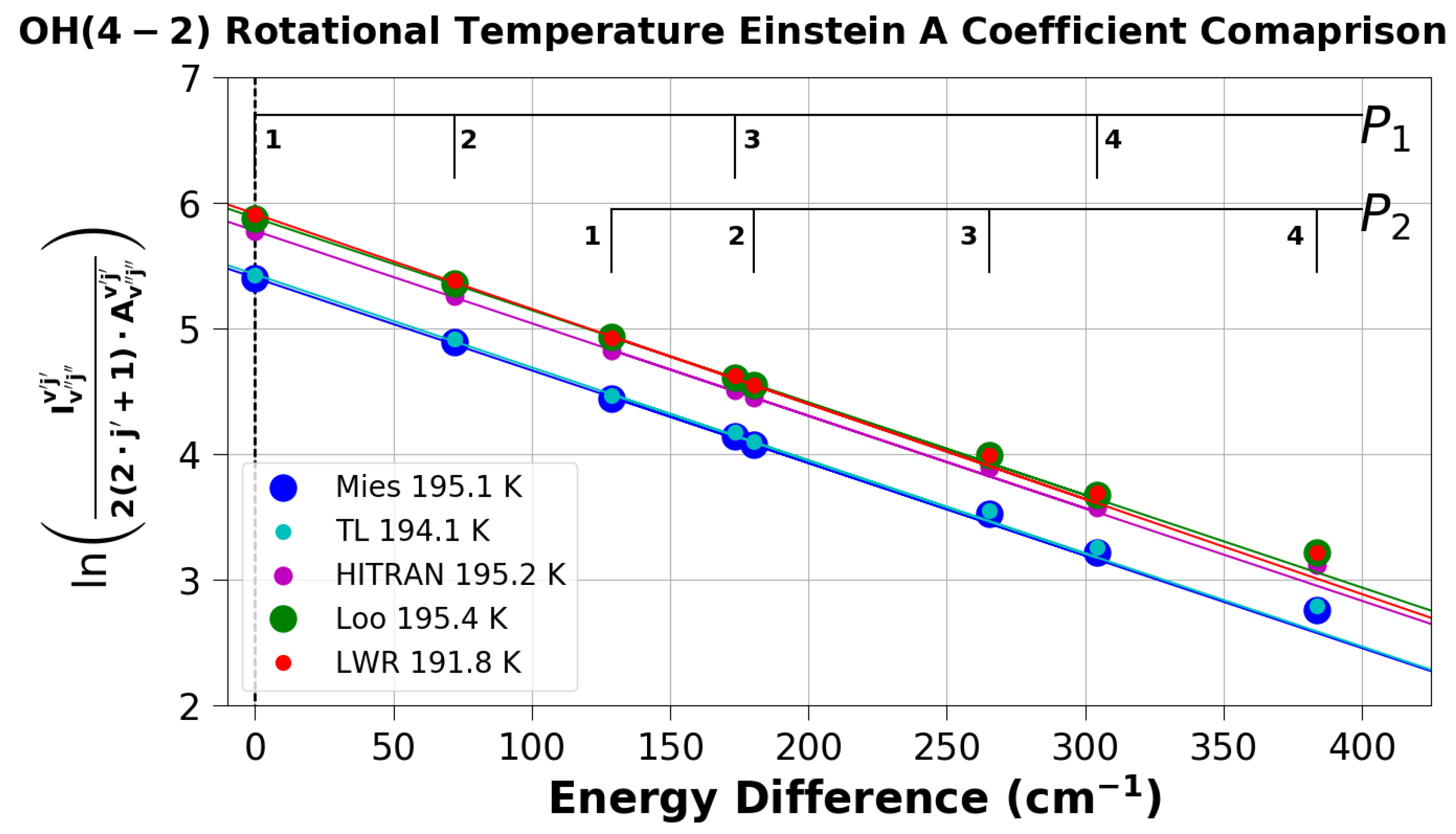
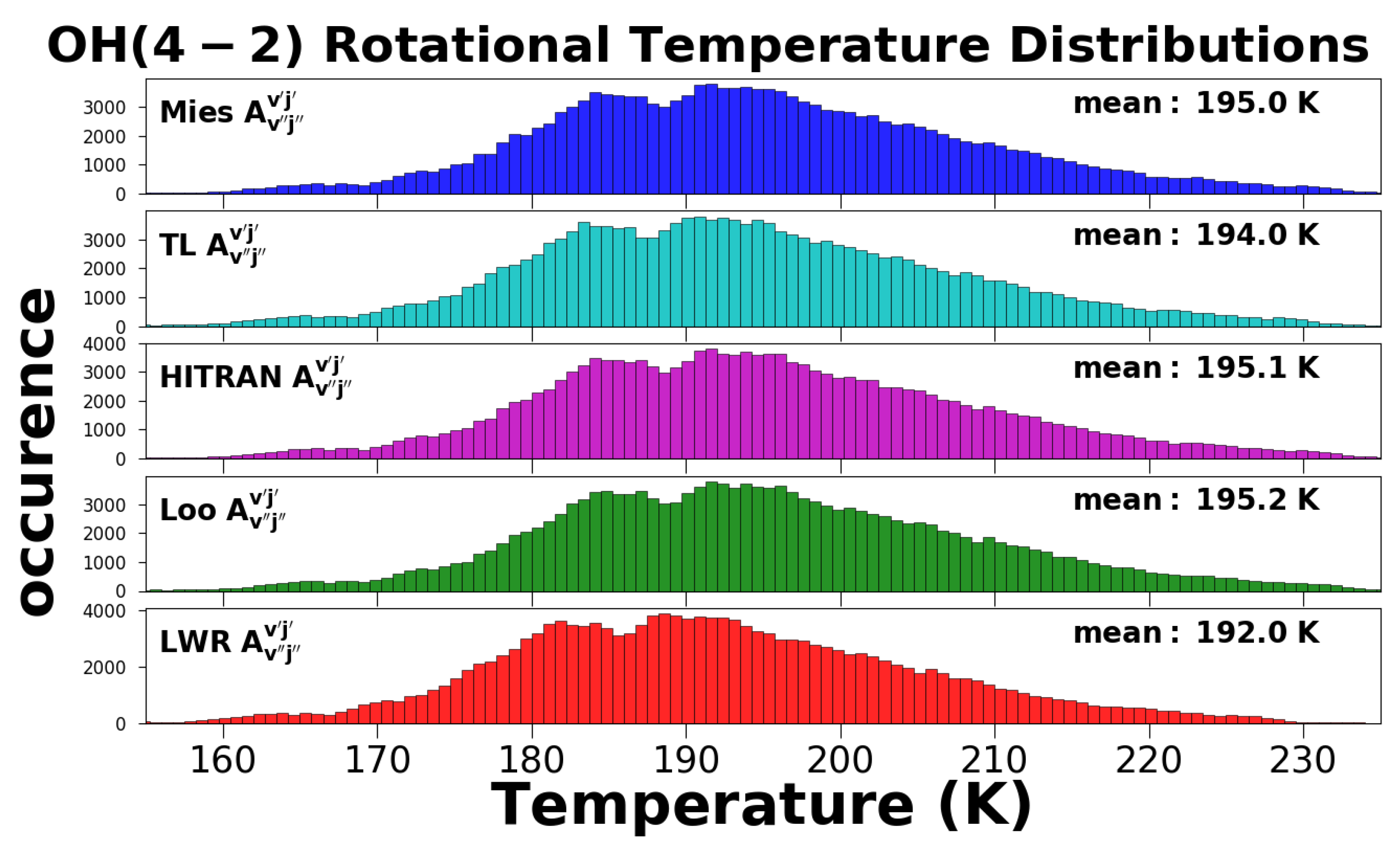
5. Einstein Coefficients
Using the selected lines from
Section 4, the
rotational temperatures were measured for the entire APOGEE dataset using five sets of Einstein
A coefficients. The Einstein
A coefficients tested were from Mies [
6], Turnbull and Lowe [
8], Rothman et al. [
17], van der Loo and Groenenboom [
16], and Langhoff [
7]. These Einstein
A coefficients will hereafter be referred to as Mies, TL, HITRAN, Loo, and LWR, respectively, and are listed in
Table 2. The distributions of measured
rotational temperatures versus Einstein
A coefficient are shown in
Figure 2, and four of the five sets of Einstein
A coefficients measured a mean
rotational temperature of approximately 195 K with only the LWR coefficients deviating significantly. The Einstein
A coefficients had a minimal impact upon the shape of the temperature distributions, but instead shifted the centers of the distributions. The distributions of APOGEE
rotational temperatures also appear to be bimodal.
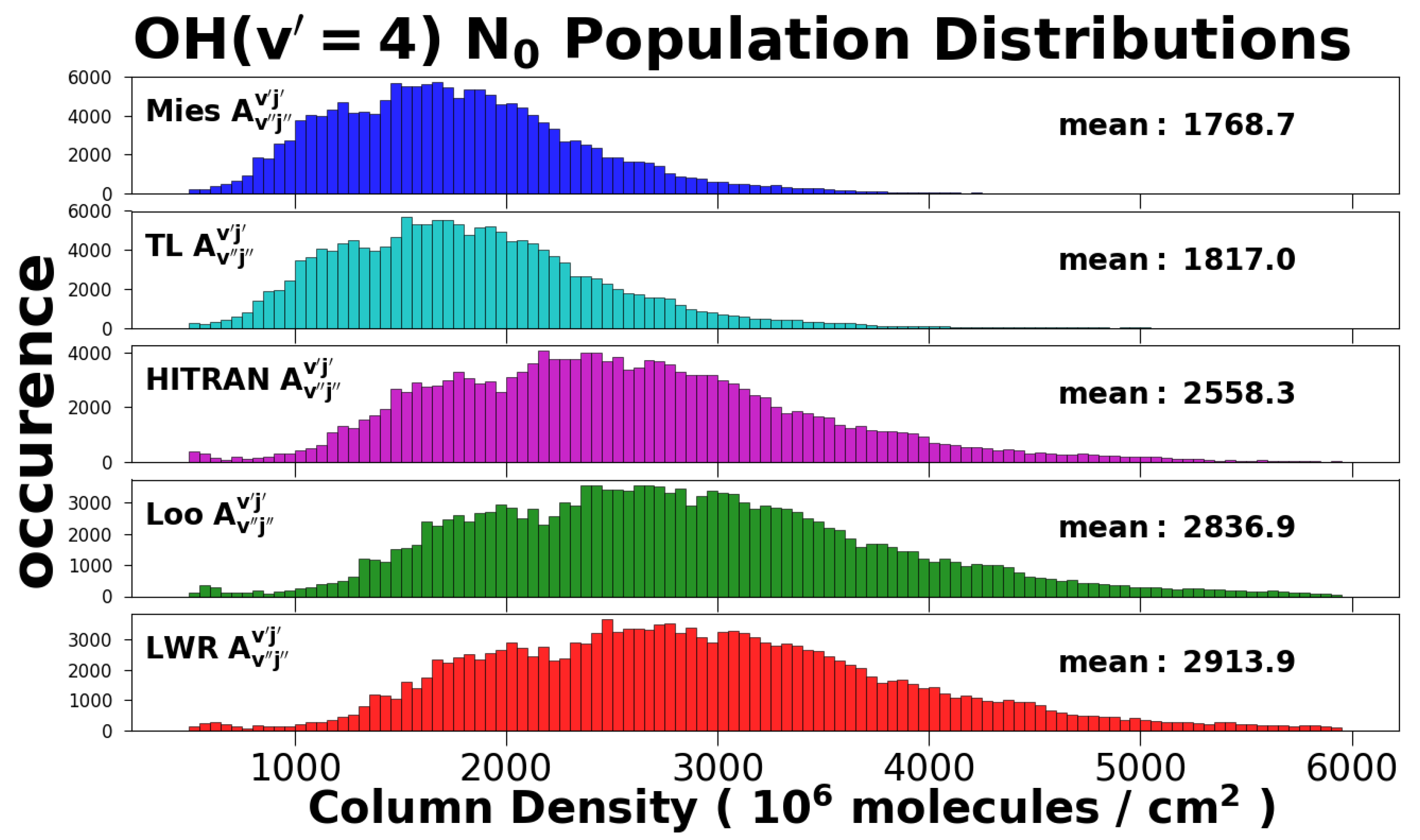
Figure 3 shows the distributions of the measured
populations for each of the Einstein
A coefficients in consideration. The
populations were derived from the intercept of the rotational temperature fit. The five sets of Einstein
A coefficients tested here yielded mean column densities which ranged from 1.7 ·
to 3 ·
molecules/cm
.
The median APOGEE
spectrum in
Figure 1 is a robust measure of the
emission above APO. The rotational temperature of the median
spectrum was calculated using the 5 sets of Einstein
A coefficients in
Figure 4. Four of the five sets of Einstein
A coefficients did not significantly impact the temperature measurement as they found a mean temperature of approximately 195 K with only the coefficients of LWR significantly deviating. It can also be seen in
Figure 4 that the
lines all show signs of enhancement due to non-LTE effects.
The Einstein
A coefficients had a significant impact upon the value of the intercept which represents the population of
.
Table 3 lists the populations calculated from the median APOGEE
spectrum in
Figure 1 using the Einstein
A coefficients from Mies, TL, HITRAN, Loo, and LWR. Line 1 of
Table 3 is the log of the population of
, and line 2 is the column density in units of
molecules/cm
. Line 3 is the ratios of the
populations normalized by
. The calculated populations of the Mies and TL coefficients differ by approximately 3%. Although the LWR and Loo populations differ by less than 10%, they are both approximately 60% greater than the populations calculated using the Mies coefficients. In
Table 1, it can be seen that the line selection did not have a significant effect upon the measured population of
.
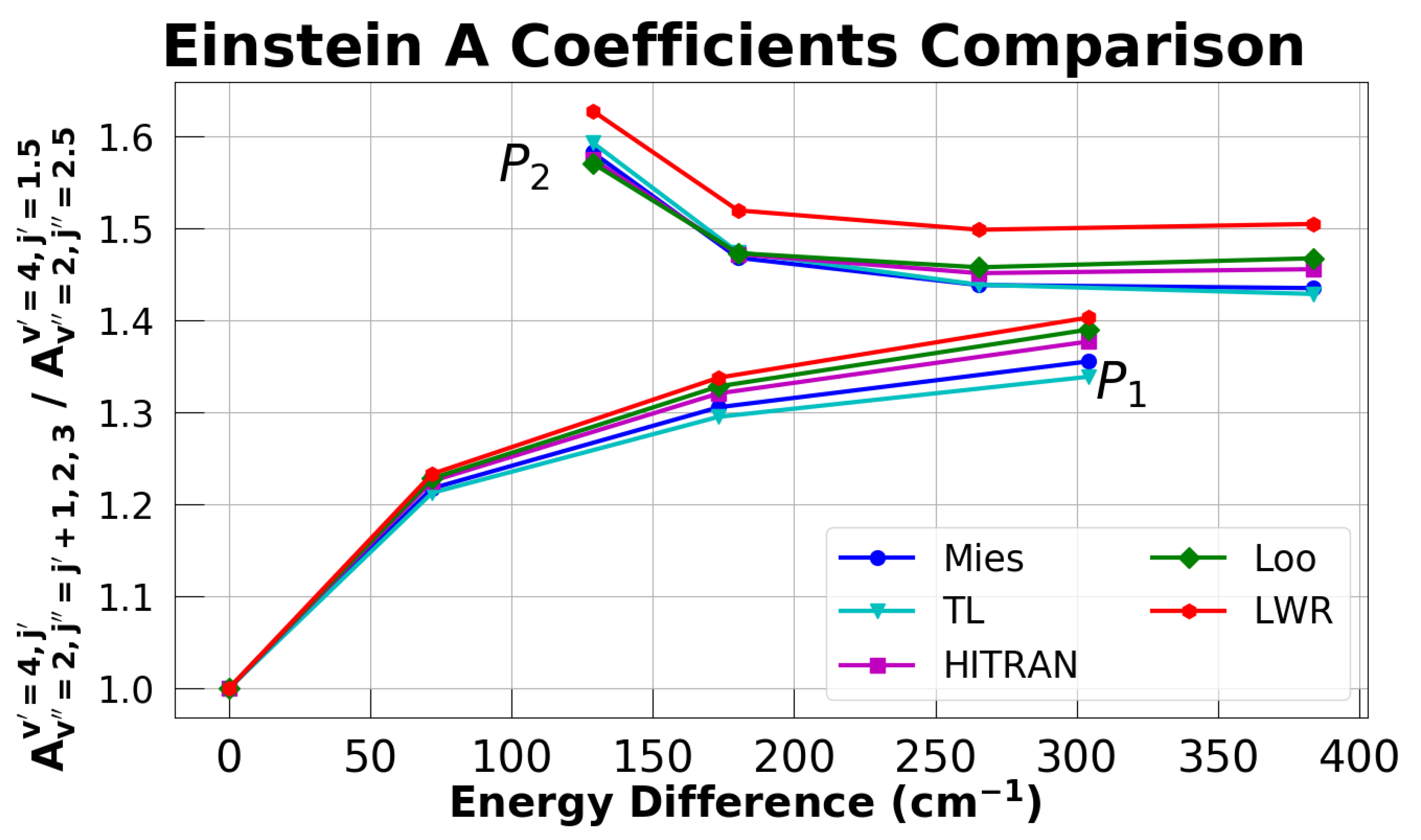
The columns of Einstein
A coefficients of Mies, TL, HITRAN, Loo, and LWR, in
Table 2, have been ordered from the largest numerically to the smallest. The Mies coefficients are the largest of the Einstein
A coefficients considered in this work, and the coefficients of LWR are the smallest. The distributions in
Figure 2 and
Figure 3 are also ordered from the largest set of coefficients to the smallest, and clear trends in the rotational temperatures and
populations are evident. The coefficients of Mies, TL, HITRAN, and Loo show little difference in mean rotational temperature while the coefficients of LWR measured lower rotational temperatures. The Mies coefficients being the largest numerically measure the lowest mean
population; in contrast, the LWR coefficients measure the largest mean
population.
Equation (
4) shows that the column density of a rotational state is inversely proportional to the Einstein
A coefficient with the larger coefficients yielding smaller column densities. The linear fit of log population to rotational energy used in rotational temperature measurements is sensitive to the ratio of the column densities and not sensitive to constant offsets. The natural log of the density is a slowly varying function which helps to minimize the differences between the sets of the Einstein
A coefficients. A change in the ratios of the coefficients translates into deviations of the slope, and the rotational temperature is inversely proportional to the slope of the linear fit.
In an attempt to gain a better understanding of the differences between the sets of Einstein
A coefficients, the coefficients were normalized by their respective
coefficient and plotted versus their corresponding rotational energy in
Figure 5. The ratios of the
coefficients of TL are always the smallest, and the ratios of LWR coefficients are the greatest. All of the
coefficient ratios increase in a way such that they do not cross the ratio of another set of coefficients. Contrastingly, the ratios of the
coefficients do cross. Ignoring the
coefficient ratios of LWR, the
coefficient ratios of Loo are the smallest at lower rotational energies and the largest at higher rotational energies. In
Figure 5, the coefficient ratios of Mies and TL are similar, as are the coefficient ratios of Loo and HITRAN. The ratio of the LWR coefficients are consistently greater than the other four coefficients in consideration, and the greater coefficient ratio translates into a lower measured rotational temperature and a larger calculated
population.
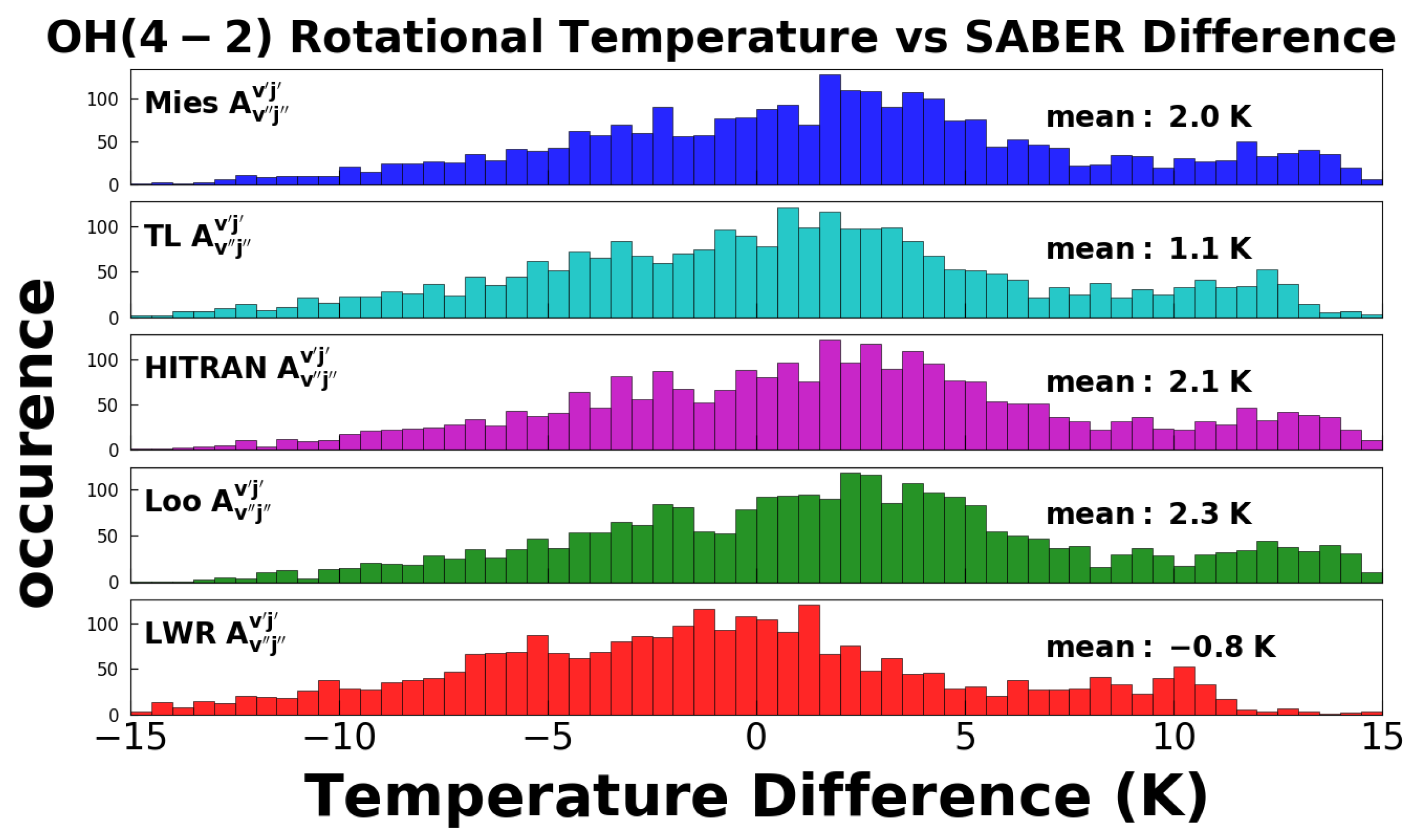
6. SABER Comparison
Ground-based
rotational temperature measurements are sampling a column of atmosphere, and in effect measure a vertical VER profile weighted average temperature. While SABER on the other hand measures a temperature profile. To allow for a proper comparison, Liu et al. [
10] weighted the SABER temperature profiles using the corresponding SABER
1.6
m VER profiles as in Equation (
5).
The altitude at which the emission peaks varies with vibrational level, and as both SABER and APOGEE sample emission from the transition the VER weighted temperatures should not be significantly biased due to differences in the altitude of emission. Small-scale spatial variations are probably still a significant source of error in comparing the two measurements as APOGEE measures a vertical column and SABER measures a vertical profile in a sweeping motion which ranges nearly 3 in latitude.
To test the accuracy of the ground-based
rotational temperature measurements, the difference between the SABER VER weighted temperatures and
rotational temperatures were calculated, and
Figure 6 shows the distribution of these temperature differences versus Einstein
A coefficient. The average temperature difference between APOGEE and SABER is approximately 1 K, and is the smallest for the Einstein
A coefficients by LWR. The APOGEE
rotational temperatures are on average higher than the SABER temperatures.
7. Discussion
Using optical SDSS spectra, Hart [
4] measured a median
rotational temperature at APO of approximately 195 K using the coefficients of van der Loo and Groenenboom [
16]. In this work, the mean APO
rotational temperature was approximately 195 K using the same coefficients. For the rotational temperature measurements the coefficients of Mies, TL, HITRAN, and Loo yielded nearly identical
rotational temperatures, and the coefficients of LWR yielded consistently lower rotational temperatures.
French et al. [
34] tested the coefficients of Mies, TL, and LWR. They determined that the coefficients of LWR best matched experimentally measured temperatures. However, French et al. [
34] used the ratio of emission lines to measure rotational temperatures, and they did not use any ratios containing an emission line from the
branch where the LWR coefficients are significantly different from the other sets of coefficients as evidenced by
Figure 5.
Measuring the rotational temperature of multiple transitions from the same upper vibrational level Noll et al. [
3] analyzed the coefficients of Goldman et al. [
9] and van der Loo and Groenenboom [
16]. They found the coefficients of Goldman et al. [
9] resulted in less scatter between the rotational temperatures derived from multiple overtones originating from the same upper vibrational level.
In this work, the average temperature difference between APOGEE and SABER was observed to be slightly greater than 1 K, with the APOGEE
rotational temperatures being predominately higher than the SABER VER weighted temperatures. Liu et al. [
10] examined the same coefficients as this work, and found the LWR coefficients most closely matched the SABER data. Using the LWR coefficients Liu et al. [
10] measured the
,
, and
rotational temperatures using the N
= 1, 2, and 3 rotational levels of the
branch, and found a positive 2.7 K, 1.4 K, and 2.1 K bias, respectively, and a positive 9.6 K bias for the
rotational temperature using the N
= 1, 2, and 4 rotational levels of the
branch. The results of Liu et al. [
10] showed a more significant differences in the calculated rotational temperatures between the Einstein
A coefficients in comparison to this work. Liu et al. [
10] found that the LWR coefficients had the smallest bias in comparison to SABER VER weighted temperatures, and an examination of
Figure 5 shows that the LWR coefficients differ significantly from the other coefficients tested in the
branch. Also all of the transitions Liu et al. [
10] compared to SABER data are from higher overtones.
French and Mulligan [
35] compared SABER temperatures to
rotational temperatures in Davis Antarctica. They found less than 2 K difference from SABER temperatures using the coefficients of LWR utilizing the same method of
rotational temperature measurement as employed in French et al. [
34]. French and Mulligan [
35] initially considered all SABER observations in which the tangent point was within 500 km of Davis, and later switched to a more restrictive 100 km and found little change in the SABER versus ground-based
rotational temperature biases. They concluded that the
layer was largely uniform over these length scales.
The five sets of Einstein
A coefficients tested in this work yielded mean
column densities which ranged from 1.7 ·
to 3 ·
molecules/cm
for the
vibrational level of the
molecule. Dodd et al. [
36] found the
column densities to be approximately 2 ·
molecules/cm
using the coefficients of Nelson et al. [
12], which are comparable to the HITRAN coefficients. Cosby and Slanger [
2] measured the
column densities to be approximately 3.5 ·
molecules/cm
using the coefficients of Goldman et al. [
9]. The coefficients of Goldman et al. [
9] with minor modifications are the HITRAN coefficients of Rothman et al. [
17].


