Fusion of High-Resolution Reflectivity for a New Array Weather Radar

Abstract

Array Weather Radar (AWR) is a novel type weather radar equipped with a distributed phased array technology. As a new instrument with new technology, the AWR offers very high spatiotemporal resolution that enables detection of the fine-scale flow field and reflectivity of severe convective storms. This new AWR provides coordinated observations of a target from three subarrays of transmitter-receiver antenna units. This paper introduces a resolution enhancement concept that the very high range resolution of one subarray can be used to compensate lower azimuth and elevation resolutions of the other subarrays of the AWR. The resolution enhancement effect is estimated using data point density. A data fusion method is then presented to obtain a unified high-resolution reflectivity from the networked and coordinated AWR subarray observations. First, based on the reflectivity data from the AWR subarray volume scans, numbers of the data-point filling in both the azimuth and elevation directions are calculated. Then, the fusion of three subarray reflectivity data is achieved through the vertical and horizontal filling and merging in a common coordinate system. The final product of the fused high-resolution reflectivity is verified using both subjective and objective evaluations. The verification experiments included radar echoes of two simulated weather scenarios, a small-scale heavy precipitation and a tornado, along with a real precipitation event. The real precipitation event was observed from the AWR system that is installed and operational at the Changsha Huanghua International Airport. The performance of the proposed high-resolution reflectivity fusion method yields a 35% smaller root mean square error and an 11% increase in the correlation coefficient to the maximum extent. The real event result shows that the final fused high-resolution reflectivity depicted a more detailed and complete echo structure compared to the China New Generation Weather Radar network observation.

1. Introduction

Meteorological disasters, such as typhoons, hail-falls, heavy rains, and tornadoes, threaten lives and properties and impact countries all over the world [1,2]. It is of great theoretical and practical significance to promote higher-level meteorological modernization and improve the reliability of meteorological monitoring and forecasting capabilities.

Weather radars have played an important role in monitoring and early warning of disastrous meso- and micro-scale weather systems [3]. However, given various types of physical environment and highly complex tracks of weather systems, the limited detection range of a single radar makes the monitoring and forecasting the movement and evolution of the entire weather systems almost impossible. The observation coverage is also reduced with increasing distances due to the radar beam broadening and beam blockage [4,5]. Moreover, at C- or X-band wavelengths, the attenuation in rains affects radar signals [6,7]. To overcome these limitations, weather radar networks have been established in different countries such as the Next Generation Weather Radar (NEXRAD) program in the United States in the 1980s, the China New Generation Weather Radar (CINRAD) network in the 1990s, and the Operational Programme for the Exchange of Weather Radar Information (OPERA) in Europe in 2000 [8,9,10].

After the deployment of the weather radar networks, a specific region is usually covered by more than one radar, from which mosaic techniques were developed to provide meso-scale weather monitoring from the networks. In 2002, the United States meteorologists proposed a mosaic technique to obtain radar products with a temporal interval of 5 min and a spatial spacing of 2 km [11]. In 2004, the China Meteorological Administration (CMA) researched on the mosaic technique for the CINRAD, which was then implemented in operation with a temporal interval of 30 min and a spatial spacing of 10 km; and in 2006, both were again improved to 6 min and 1 km, respectively [12]. In the same year, a technique for generating three-dimensional (3D) merged grid product in real time was implemented, which was based on an intelligent agent formulation and led to an enhanced temporal interval of 1 min and a spatial spacing of 1 km [13]. In 2014, an inverse method assuming the models for the radar sampling of the atmosphere and path attenuation was proposed to obtain 3D reflectivity composites with the grid spacing of 500 × 500 × 250 m³ [14]. In general, the most commonly used techniques are based on the nearest neighbor method, the maximum value method, the weighted average method, or the arithmetic average method [15,16,17]. One method cannot be suitable for all conditions, different methods are proposed and selected for specific applications [18].

Due to the propagation characteristics of electromagnetic waves, different wave-length (band) radars have different performance limitations. Normal long-range S-band Doppler radars, such as the NEXRAD and the CINRAD radars, have blind detection areas at low altitudes due to the earth curvature effects and low volume update rates in the monitoring of small-scale severe convective storms. Furthermore, the atmospheric conditions and the scanning time difference between radars can also bring detection errors [19]. With the development of radar technology, X-band weather radars have been widely used in meteorological detection. To solve these problems, the concept of networked and coordinated weather radars, utilizing the low-power and low-cost X-band radars, has been proposed [20]. The coordinated radars observe in a Distributed Collaborative Adaptive Sensing (DCAS) mode and focus on the same concerned target area [21]. As an example, the National Science Foundation established the Collaborative Adaptive Sensing of the Atmosphere (CASA) Engineering Research Center in the United States in 2003 [22]. The first integrative project (IP1) consisted of four radars located in Oklahoma, spaced nearly equidistantly at 25 km apart. This CASA DCAS system was able to provide high spatiotemporal resolution and fill up the blind detection areas of the existing long-range radar system [23,24]. The maximum operating range of each CASA IP1 radar was 30 km, and the spatiotemporal resolutions were 100 m and 60 s, respectively [25].

In 2013, a CASA-like networked X-band weather radar system was first established in China by the Institute of Atmospheric Physics of the Chinese Academy of Sciences and Nanjing NRIET Co. Ltd. of the China Electronics Technology Group Corporation, with the participation of the Meteorological Observation Center and the Chinese Academy of Meteorological Sciences of CMA. This networked radar system consists of four X-band weather radars, forming a diamond-shaped distribution. The effective detection range is 60 km in and around Nanjing, China, with the temporal resolution of 2 min [26].

In 2015, Japan established the Osaka Urban Phased Array Radar Demonstration Network, which provides products such as reflectivity, vertical integrated liquid water content, and precipitation rate in real time [27]. It was the first time in the history of the weather radars that two short-range phased array radars were used to form a Phased Array Radar Network, which mitigates the shortcomings such as large time difference and a low scan speed of traditional weather radar systems. It represents a new development in the field of weather radar networks and further provides a future direction to fine-detection weather radar development [28].

In 2015, the Array Weather Radar (AWR) concept was proposed and designed by the Meteorological Observation Center of the CMA [29]. In April 2018, the first AWR with three subarrays of transmitter-receiver antenna units, which are abbreviated as subarrays in this paper, was built by Hunan Eastone Washon Science and Technology Co. Ltd. It was deployed at Changsha Huanghua International Airport for carrying out field observation experiments [29]. It is similar to the weather radar network composed of the phased array weather radars in Osaka, Japan in that a phased array radar technology is adopted. The difference is that the AWR must have at least three phased array subarrays as a group to complete coordinated (or collaborative) observations. A full coverage detection of the AWR that scans 0°–90° in elevation angles and 0°–360° in azimuth angles requires only 12 s. Therefore, the AWR has the advantage that a full 3D wind field can be retrieved from its three subarray radial winds and a high-resolution reflectivity field can be fused from the reflectivity of all three subarrays.

This paper is organized as follows: In Section 2, an overview of the AWR is provided. The principles of the resolution enhancement and procedures of the AWR high-resolution reflectivity fusion method are described in Section 3. Performance evaluations of the two simulated reflectivity fusion and one real precipitation event are presented in Section 4. The main conclusions of this paper are summarized in Section 5.

2. Array Weather Radar

As discussed above, existing weather radars are facing a difficulty in obtaining fine-scale weather features that change rapidly in time and space, such as tornadoes, hail-storms, and convective precipitations [30]. Short-range phased array weather radars developed in recent years have enhanced the temporal resolution of detection, but can only measure the radial velocity of precipitation particles along the radar beam. The networked weather radar system, on the other hand, can acquire the radial velocity field of a slow-moving weather system, but cannot acquire the real flow field of a rapidly and strongly changing weather phenomena because of the large time differences among different radars [31]. The AWR is a distributed, highly coordinated phased array weather radar that combines the advantages of both the phased array weather radar and the networked weather radar systems. It can achieve full coverage in space and greatly enhance the spatiotemporal resolution as well. Therefore, the AWR can achieve a complete detection of precipitation particle motion by obtaining both 3D real velocity and reflectivity. It is a powerful tool for assisting in-depth research of fine-scale weather systems and in real-time surveillance tasks.

The AWR is designed to have at least three phased array subarrays. The subarrays use a phased array digital beamforming technology for electronically generating four transmitting beams, covering elevation angles of 0°–22.5°, 22.5°–45°, 45°–67.5°, and 67.5°–90°, and forming 64 receiving beams with an average beamwidth of 1.6°, implying overlapped beams in the elevation direction. Meanwhile, the 0°–360° azimuths are covered via mechanical scans. Every subarray is composed of an antenna array, a transmitter-receiver module array, a signal processor array, an azimuth rotation servo unit, and a battery module. The three subarrays are arranged at the vertices of an acute triangle (an equilateral triangle should be ideal) as shown in the schematic diagram in Figure 1. The three subarrays scan a fine detection area collaboratively, and the time difference of scans of the same spatial point from different subarrays is about 2 s (2 s for an equilateral triangle). The subarrays can also detect weather in the medium detection area that is covered by only two subarrays and in the normal detection areas that is covered by only one subarray. The main technical specifications of the AWR in Changsha are shown in

Table 1. Main technical specifications of the AWR in Changsha.

Indicators	Main Technical Specifications
Technology	Distributed phased array
Frequency range	X-band
Range resolution	30 m
Maximum effective range of a single subarray	20.28 km
Number of data bins in one volume scan	64 × 240 × 676
Distances between subarrays	20–60 km
Azimuth and elevation beamwidth	1.6°
Antenna scan mode and range (azimuth)	0°–360°, mechanical scan
Antenna scan mode and range (elevation)	0°–90°, electronic scan
Fine detection subzone scan time	2 s
One volume scan time	12 s

. The maximum effective range of each subarray is about 20 km. The number of data bins in one volume scan is about 64 × 240 × 676 (elevation, azimuth, and radial direction numbers, respectively), given overlapped beams in azimuth and elevation directions. The whole processing flow have been implemented and optimized on NVIDIA (one of the leading GPU suppliers) GPU architecture in real-time tasks.

3. AWR High-Resolution Reflectivity Fusion Method

3.1. Basic Principle

The weather radar resolutions usually refer to the temporal resolution and spatial resolution [32]. The temporal resolutions are generally determined by the radar scanning modes, which are basically affected by the speed of mechanical rotation of antenna and the azimuth scanning range. The spatial resolutions include the range (distance from radar) resolution, azimuth resolution, and elevation resolution. The radar detected energy is the sum of scattered energy by all the particles within a 3D volume (bin) of the size of azimuth resolution, elevation resolution, and range resolution in the three directions, respectively. In the practice of data processing, sometimes the center point of each bin is used as a data point to approximately represent the bin, which can be defined by an azimuth, an elevation, and a range [33]. The range resolution is determined by the transmitted pulse width and the receiver filter, and thus is constant. The azimuth and elevation resolutions are determined by the radar beamwidth of the antenna. Both the azimuth and elevation resolutions reduce (or the size of resolvable data bin increases) with the increasing detection distance [34]. For example, for the 1.6° azimuth beamwidth and when the detection range change from 10 km to 20 km, the lateral dimension of the resolution volume increases from 279 m to 558 m, while the range resolution is kept at 30 m.

To obtain a higher azimuth resolution at a greater detection distance, a direct method is to increase the antenna size or reduce the pulse width. It means that the antenna, the transmitter and the receiver need to be upgraded, which is not an optimum solution considering their high costs. In this paper and with the AWR, there are three subarrays operating in a coordinated manner of detection, providing three reflectivity observations from three different directions. The very high range resolution of one subarray can actually compensate for the low azimuth and elevation resolutions of the other two subarrays. Figure 2 shows a schematic diagram of two crossed beams from two subarrays for detecting the same area from different viewing angles and illustrates how the overall resolution can be enhanced. As shown, the gray-colored data bin is detected by the subarray 1. As demonstrated above for the resolutions, if this bin is 20 km away from subarray 1, its dimensions in range and azimuth are about 30 m × 558 m. Note that subarray 1 has only one detected value in the entire bin (the gray-colored region for the two-dimensional (2D) view). Now at the same time, through the coordinated detection of the subarray 2 from another direction, the gray-colored data bin of the subarray 1 is partially detected by many data bins of the subarray 2 along its range direction. These many data bins of subarray 2 supplements more details for the subarray 1 data bin in its azimuth direction, along which only one data was available from subarray 1. Taking the example of the 20 km range location of subarray 1, the gray-colored data bin is supplemented by information from about 19 data bins of subarray 2 at the same distance. With appropriate data fusion schemes, it is expected that the overall resolution of detection can be enhanced by using data from two or more subarrays. Thus, a more detailed and complete weather echo structure may be obtained.

3.2. Estimation of Resolution Enhancement

In this section, we further estimate resolution enhancement effects quantitatively. Resolution is usually defined as the spatial or temporal distance of smallest and adjacent resolvable units. In case of radar azimuth and elevation resolutions, it is usually the beamwidth measured in angular degrees. Resolution can also be measured in the number of data bins that intersect with or fall into a unit volume (3D) or unit area (2D). When the center of each data bin is used as an approximate data point, this measure is essentially data point density, which is used below to investigate the resolution enhancement of the AWR. Figure 3 shows a 2D schematic diagram of how the data point density can be calculated. The red-box area represents a unit area, into which some data points (red circles) of the subarray fall. The unit area is preset with known coordinates. Using the same coordinate system and origin, the coordinates of each data point are calculated according to the latitude and longitude of all subarrays. If a data point falls into the unit area, it is recorded as a valid point. The number of all valid points is the data point density.

To further explain the idea of using the range resolution to compensate the azimuth resolution and the resolution enhancement effect evidently, a data point density estimation experiment of two perpendicular subarrays are completed and the experiment results are shown in Figure 4. The two subarrays are perpendicular to the target for the optimal compensation effect, and the size of the target area is 6 km × 6 km (each pixel in Figure 4 represents 30 m × 30 m). Two subarrays are set at the west (subarray 1) and the south (subarray 2) of the same target area to scan respectively with the same distance of 5 km (the distance from radar to the near side of the target area). Each data point along the radial direction shown in Figure 4a,b represents the center point of a bin. Note that due to the 30 m range resolution, the dots are very close to each other along the radial direction but far apart in the azimuth direction. When this target area is scanned by both subarrays, the data point distribution map of this target area is shown in Figure 4c. The target area is divided into nine parts to analyze the distribution of the resolution enhancement effect for the entire target area. From the subjective evaluation, the density in the lower left part is significantly higher than in the other parts, which means the echo structure in the lower left part is finer than in the other parts (see Figure 4c). To objectively evaluate the resolution enhancement effect, Figure 4d–f show the data point density corresponding to Figure 4a–c scanned by subarray 1, subarray 2, and both subarrays, respectively. It is clearly shown in Figure 4f that the data point density in the lower left part scanned by both subarrays is higher than in all other parts. If the third subarray is added to the northeast of the target area, the data point density of the nine parts will tend to have more even distributions as shown in Figure 5.

3.3. Fusion Procedures

The high-resolution reflectivity fusion method mainly comprises three steps which are described in detail in this section. Before the fusion, reflectivity data need to be preprocessed, including quality control, ground clutter removal, and attenuation correction.

Step 1. Calculating the numbers of data-point filling in the azimuth and elevation directions. As discussed earlier, one subarray’s high range resolution compensates the azimuth resolution of the other subarray. To prepare data for fusion in the step 3 below, we first fill more data points along the azimuth and elevation directions. The number of data points to be filled in a data bin can be calculated as:

$$N=\frac{\theta ·R}{r}$$

(1)

where N is the number of points to be filled in, θ is the azimuth or elevation resolution (in radians), R is the range along the radial direction between the subarray and current data bin, and r is the range resolution of the subarray.

Step 2. Filling reflectivity data points in azimuth and elevation directions. The azimuth filling method is shown in Figure 6a, which is similar to a linear interpolation along the azimuth direction. When the reflectivity values of two azimuthally adjacent data bins are known as Z₁ and Z₂, the N filling data values a₁, a₂, …, a_N, can be calculated by:

$$a_n=\frac{(Z_2-Z_1)}{N}·n+Z_1\left(n=1,2,\dots ,N\right)$$

(2)

The elevation filling method is shown in Figure 6b, which is similar to taking the nearest neighbor method [35], since the AWR is configured with overlapped beams in elevation direction. Although the beamwidth is 1.6°, there are 64 beams within the 0°–90° elevation range, and thus, higher effective elevation resolution. For given two adjacent reflectivity values of Z₁ and Z₂ in elevation, the N data values to be filled between the adjacent two elevations are divided into two parts. The points that are close to the location of Z₁ will be filled with the value Z₁, and the points that are close to the location of Z₂ will be filled with the value Z₂.

Step 3. High-resolution reflectivity fusion. Before fusing AWR reflectivity, we interpolate the reflectivity of all subarrays onto the same Cartesian grid according to their latitude, longitude, and altitude information. The final fused reflectivity at a given grid point i (in Cartesian coordinate) is the average of the reflectivity values at this grid point from all of the subarrays. It is expressed as:

$$Z=\frac{{\sum }_{i=1}^{num}{Z}_i}{num}$$

(3)

where Z is the fused high-resolution reflectivity value in dBZ, Z_i is the reflectivity detected by the subarray i, and num is the total number of the AWR subarrays.

4. The Simulated Subarray Scan Process and Performance Analysis

The performance of the reflectivity fusion is first evaluated both subjectively and objectively using simulated subarray scans. Because of the limited radar resolutions in all existing radars, there is no real-case small-scale severe storm echoes that can be used for this evaluation. Therefore, two simulated storms, including a heavy precipitation and a tornado, are constructed and used in this paper as the ’truth’ echoes [36]. Through such echoes with obvious characteristics, the fusion performance can be evaluated and demonstrated more clearly. In the meantime, only 2D reflectivity fields for these two simulated events are constructed, and the discussion below is focused on the range and azimuth directions only. The heavy precipitation echo was constructed based on a real convective event captured by one subarray of the AWR; the tornado echo is constructed from a modified and miniaturized real typhoon dataset.

The performance analysis comprises the following three steps. Firstly, two subarrays are simulated to scan the above constructed severe storms simultaneously. Then, the high-resolution reflectivity fusion is performed. Finally, after comparing the fused reflectivity with the ’truth’ echoes, the reflectivity fusion performance is evaluated in terms of correlation coefficient (CC) and root mean square error (RMSE) [37]. The three steps are further described as follows.

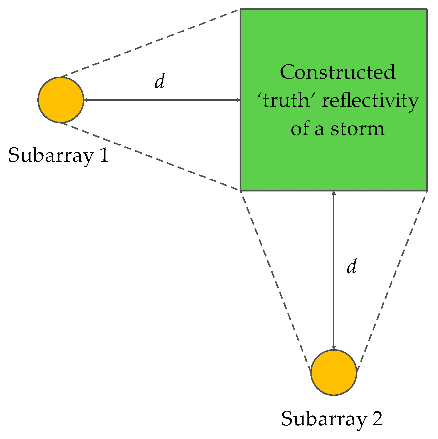
In the simulated scanning processes, the two subarrays scan the same storm simultaneously as shown in Figure 7. The subarrays are set at the west (subarray 1) and the south (subarray 2) of the same storm to be scanned, respectively. In order to reveal the influences caused by different distances between the storm and the two subarrays, different distances including 5 km, 10 km, and 20 km were experimented with, as described in Section 4.1 and Section 4.2. 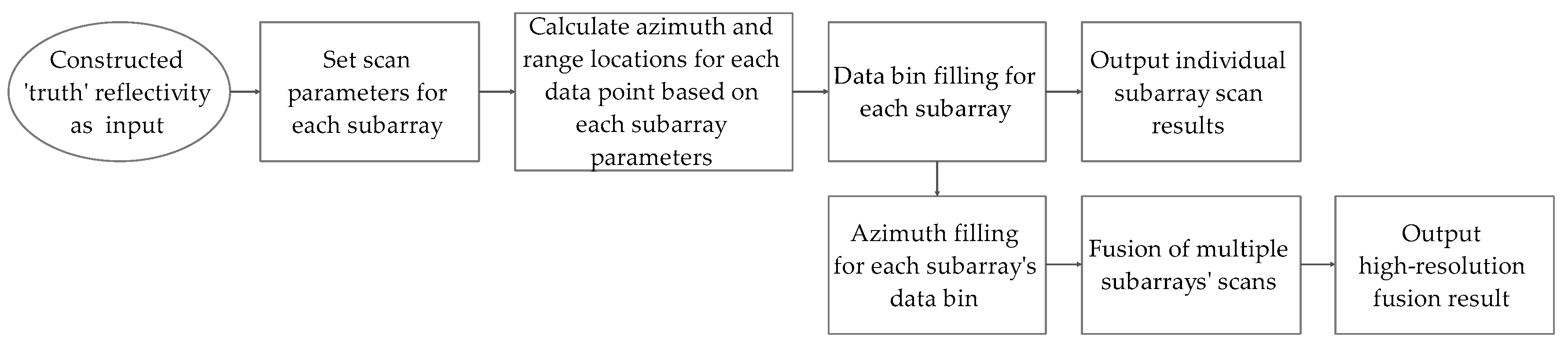Figure 8 shows a flow diagram detailing the process of simulated subarray scans. First, the constructed ‘truth’ reflectivity data of a storm event are used as input, and the scanning parameters of a subarray are set. The azimuth beamwidth of the subarrays is set at 1.6° and the range resolution is set at 30 m. Then, for each data point in the ‘truth’ field, the azimuth and range locations are first calculated to determine which data bin of a subarray this data point belongs to. Finally, to obtain the individual subarray scan results, each data bin is filled with the average value of all the data points that fall in the same data bin. This simulated scanning process of the subarray scans is indeed similar to a downsampling process. With the simulated subarray scan data, the fusion procedures described in the previous section are carried out, from which the 2D high-resolution fused reflectivity can be obtained.

To objectively evaluate the quality of the fused reflectivity, the CC and RMSE metrics are used. They are calculated by:

$$\mathrm{CC}=\sqrt{\frac{\mathrm{Cov}\left(Z_{\mathrm{o}},Z_{\mathrm{t}}\right)}{S\left(Z_{\mathrm{o}}\right)S\left(Z_{\mathrm{t}}\right)}}$$

(4)

$$\mathrm{RMSE}=\sqrt{\frac{\sum {(Z_{\mathrm{o}}-Z_{\mathrm{t}})}^2}{n}}$$

(5)

where Z_o is the reflectivity from simulated subarray scans, which is treated as ‘observations’ in the experiments and can either be scans from a single subarray or the fusion of multiple subarrays, Z_t is the ‘truth’ reflectivity, Cov represents covariance of Z_o and Z_t, S represents standard deviation, and n is the total valid number of data points. When the CC is close to 1, the similarity between the Z_o and Z_t is high, which means high consistency between the two fields. Lower RMSE means smaller difference between the two fields.

4.1. Simulated Scan of Heavy Precipitation and Performance Analysis

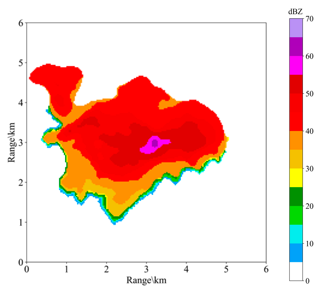
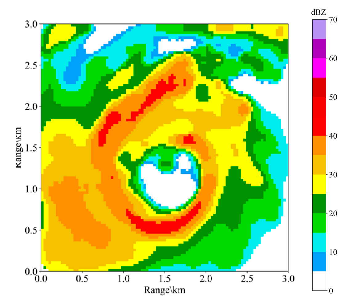
The ‘truth’ reflectivity of the heavy precipitation is shown in Figure 9. The size of the entire precipitation area is about 6 km × 6 km. Each data point in Figure 9 represents reflectivity of a 30 m × 30 m area, meaning the spatial resolution of this ‘truth’ data is 30 m × 30 m. There is mainly only one precipitation center, and the highest reflectivity reaches 64 dBZ.

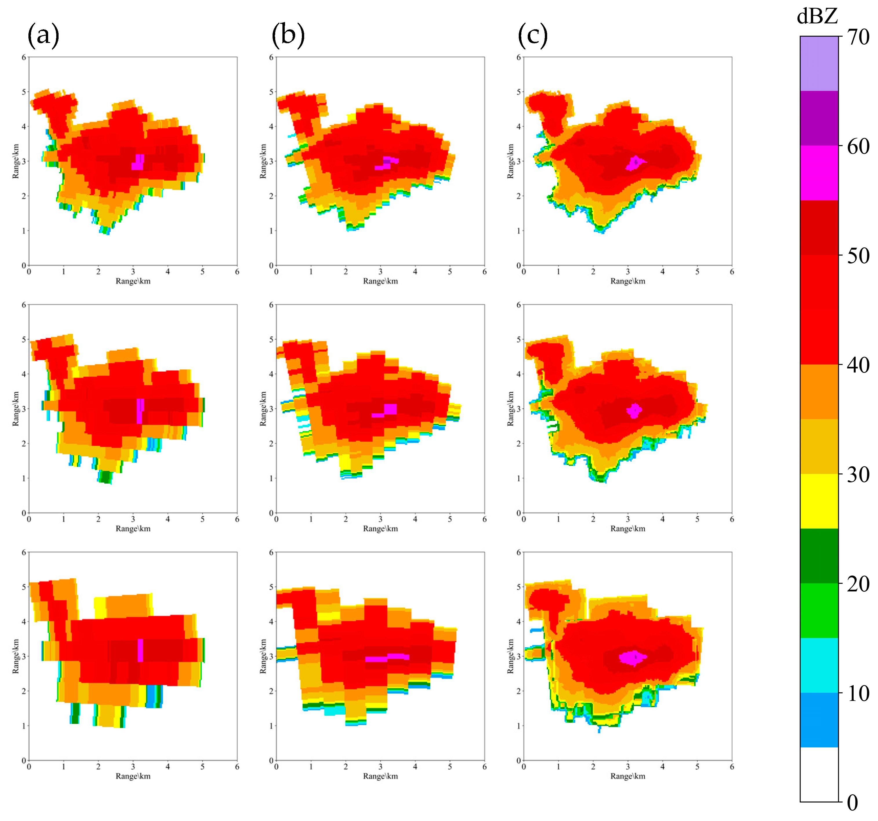
Figure 10a,b show the simulated subarray scan results by the subarray 1 and subarray 2, respectively, from three different distances (panels from the top down are for 5 km, 10 km, and 20 km, respectively). Figure 10c shows the fused reflectivity from both subarrays also from three different distances (from top down for 5 km, 10 km, and 20 km, respectively). From a subjective evaluation on the simulated scan performance, the subarrays 1 and 2 at the distances of 5 km and 10 km captured the center of the heavy precipitation, and the echo structure is generally consistent with the ‘truth’ echo in Figure 9. However, since the azimuth resolution is reduced with the increased observing distance, the individual subarrays scanning from 20 km distance have a large degree of tangential blurring effect. In comparison, the fused reflectivity fields in Figure 10c are more consistent with the ‘truth’ echo. The fusion not only restores the center of the echo when observed from all three distances, but also makes the precipitation levels more clear and vivid, and depicts these with higher fidelity.

The results of quantitative evaluation of the reflectivity obtained by each individual subarray and the fused high-resolution reflectivity are shown in

Table 2. Evaluation of the simulated heavy precipitation scans. CC: Correlation coefficient; RMSE: root mean square error.

	Parameters	5 km	10 km	20 km
Subarray 1	CC	0.93	0.89	0.79
	RMSE (dB)	3.26	4.14	5.50
Subarray 2	CC	0.94	0.92	0.87
	RMSE (dB)	2.99	3.58	4.36
Fusion	CC	0.97	0.94	0.88
	RMSE (dB)	2.15	3.19	4.36

, compared to the ‘truth’ echo in Figure 9. The most noticeable observation is that the fused high-resolution reflectivity data all have the highest CC value and the lowest RMSE value, compared to each individual subarrays and regardless of observing distance. Nevertheless, the CC value decreases and the RMSE value increases with the increasing observing distance. The fusion reduced the RMSE value of subarray 1 by 34% and of subarray 2 by 28% for the observing distance of 5 km, while it increased the CC value by 11% for the distance of 20 km. The subarray 2 shows slightly better results than the subarray 1, which is likely due to the precipitation area being slightly west-eastward oriented and thus the decrease of azimuth resolution with increasing range had smaller impact.

4.2. Simulated Scan of Tornado and Performance Analysis

Figure 11 shows the reflectivity of the simulated tornado, which is again used as the ‘truth’ echo. The size of the tornado is 3 km × 3 km and the eye shown on the reflectivity field is about 0.5 km × 0.5 km. Each data point in Figure 11 represents the reflectivity of a 30 m × 30 m area [38].

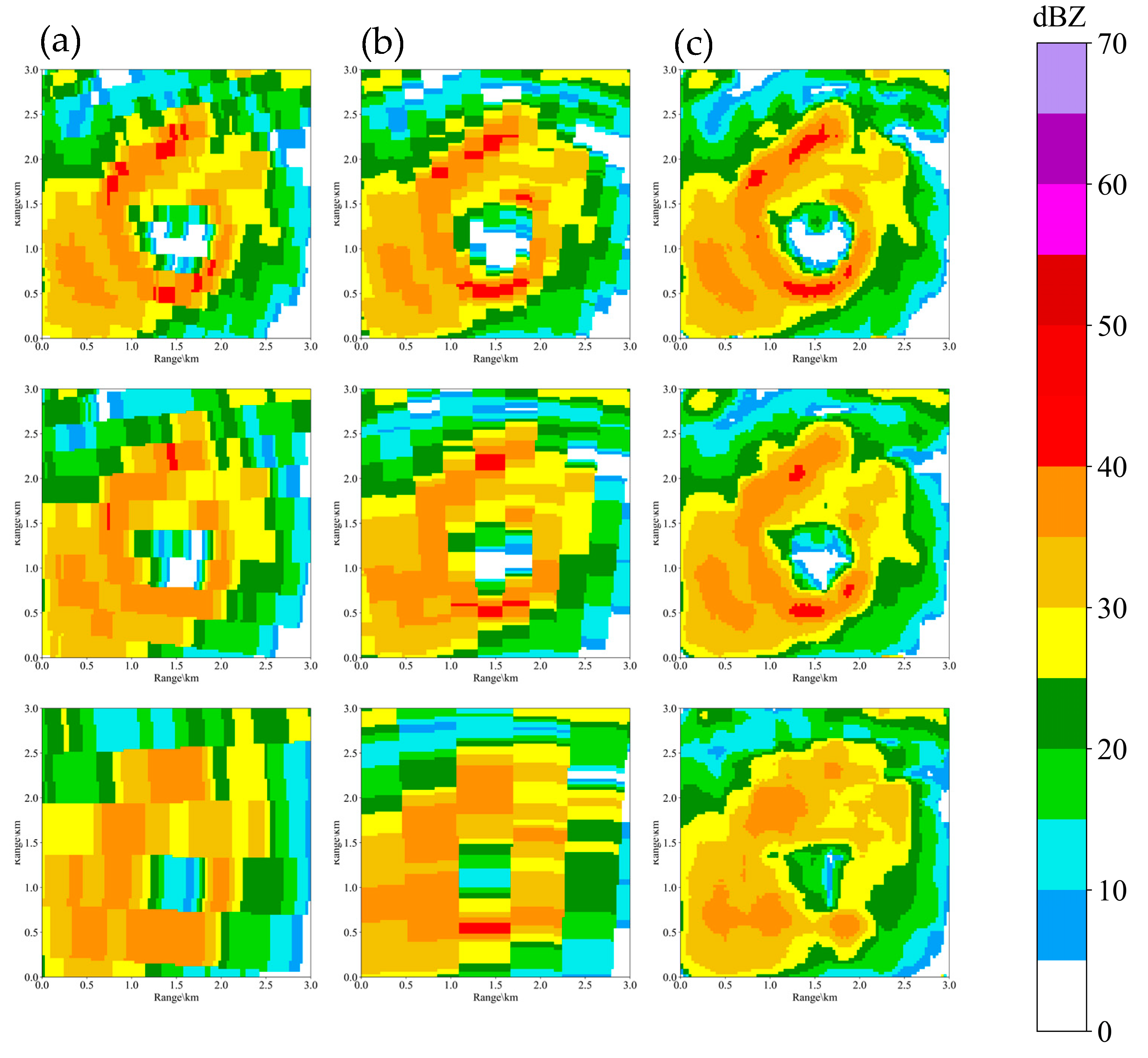
The evaluation procedures are the same as for the heavy precipitation case, and a figure similar to Figure 10 is shown in Figure 12 for the simulated tornado case. Overall, a subjective evaluation suggests that, as the distance increases, the performance of the echo structure detection decreases. At the observing distance of 20 km, neither of the subarrays can detect the eye of the tornado. However, the echo structures of the fused high-resolution reflectivity are most similar to the ‘truth’ echo from all distances (Figure 12c), even from the 20 km distance, a weak eye can be seen.

Similarly, the quantitative evaluation results for the tornado detection are shown in

Table 3. Evaluation of the simulated tornado scans.

	Parameters	5 km	10 km	20 km
Subarray 1	CC	0.96	0.91	0.82
	RMSE (dB)	2.55	3.86	5.47
Subarray 2	CC	0.97	0.94	0.85
	RMSE (dB)	2.40	3.24	5.08
Fusion	CC	0.98	0.96	0.89
	RMSE (dB)	1.65	2.67	4.25

. Compared to individual subarrays, the fused high-resolution reflectivity data all have the highest CC value and the lowest RMSE value, as concluded in the precipitation case. The fusion reduced the RMSE value of subarray 1 by 35% and of subarray 2 by 31% for the observing distance of 5 km. The maximum 9% increase of the CC value is found from the observing distance of 20 km. Again, the subarray 2 had slightly better results than the subarray 1.

4.3. Implementation of High-Resolution Reflectivity Fusion on a Real Precipitation Event

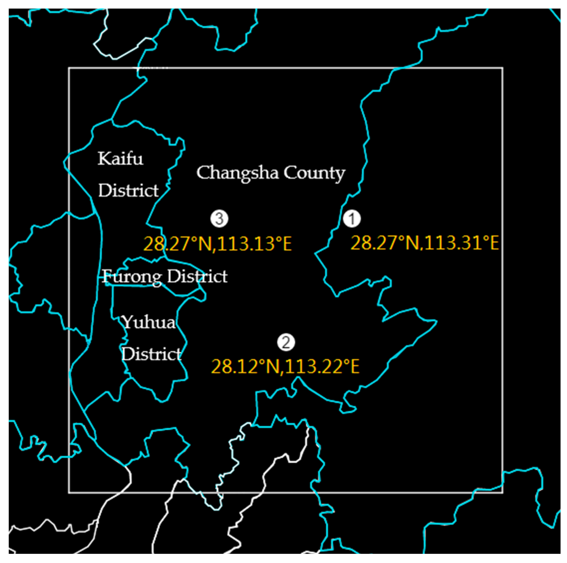
A precipitation event occurred from 05:30 to 07:00 UTC on 15 August 2018 in the neighboring area of Changsha Huanghua International Airport. The precipitation echoes captured by the AWR moved toward the southwest, with the echo top at 10 km height. The horizontal size of the precipitation cell is approximately 30 km in diameter. In this paper, the AWR detection data at 05:49:12 UTC 15 August 2018 are selected for high-resolution reflectivity fusion. The layout of three subarrays of the AWR at Changsha airport is shown in Figure 13. The AWR fused reflectivity was generated with a grid spacing of 100 × 100 × 100 m³.

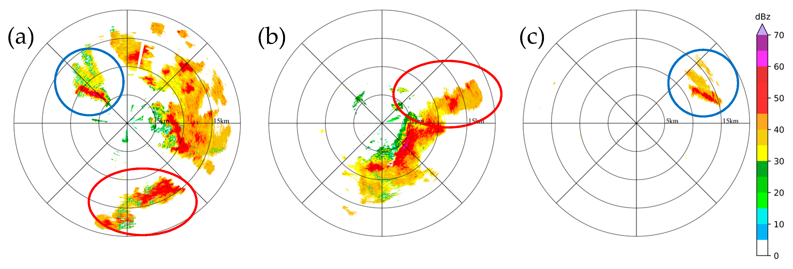
The Plan Position Indicator (PPI) display from the three subarrays of the AWR at 05:49:12 UTC 15 August 2018 are shown in Figure 14. The subarray 1 and 2 have a common detection area, which is shown in the red circle area in Figure 14a,b; the subarray 1 and 3 have a common detection area, which is shown in the blue circle area in Figure 14a,c.

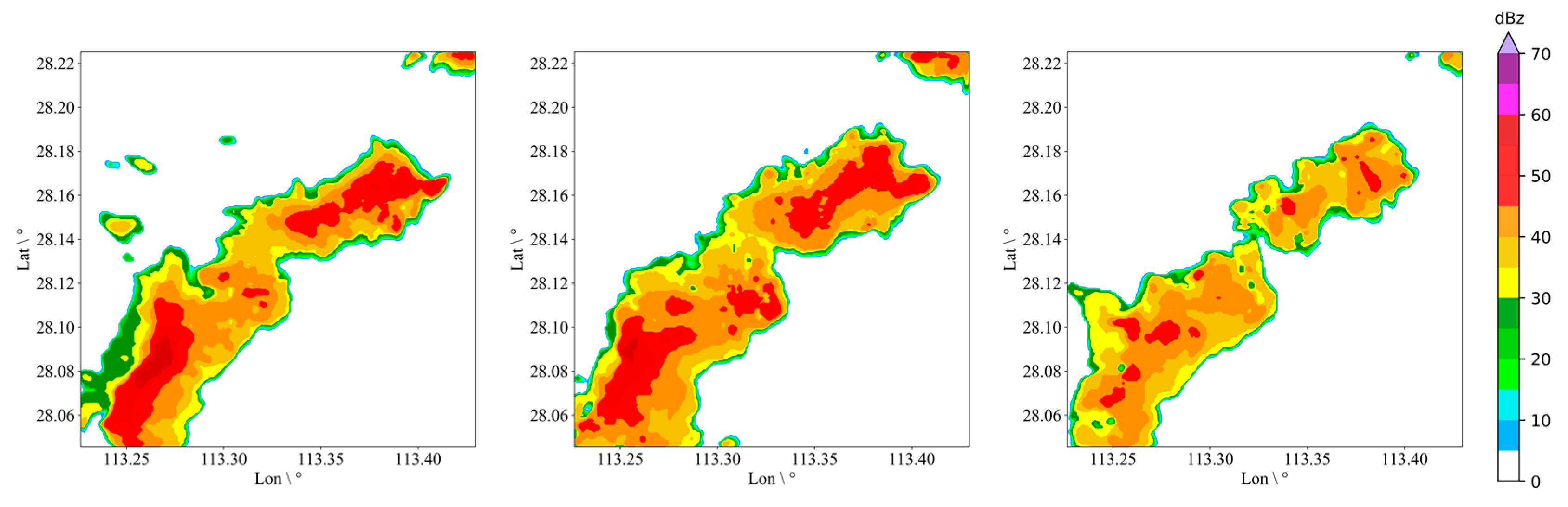
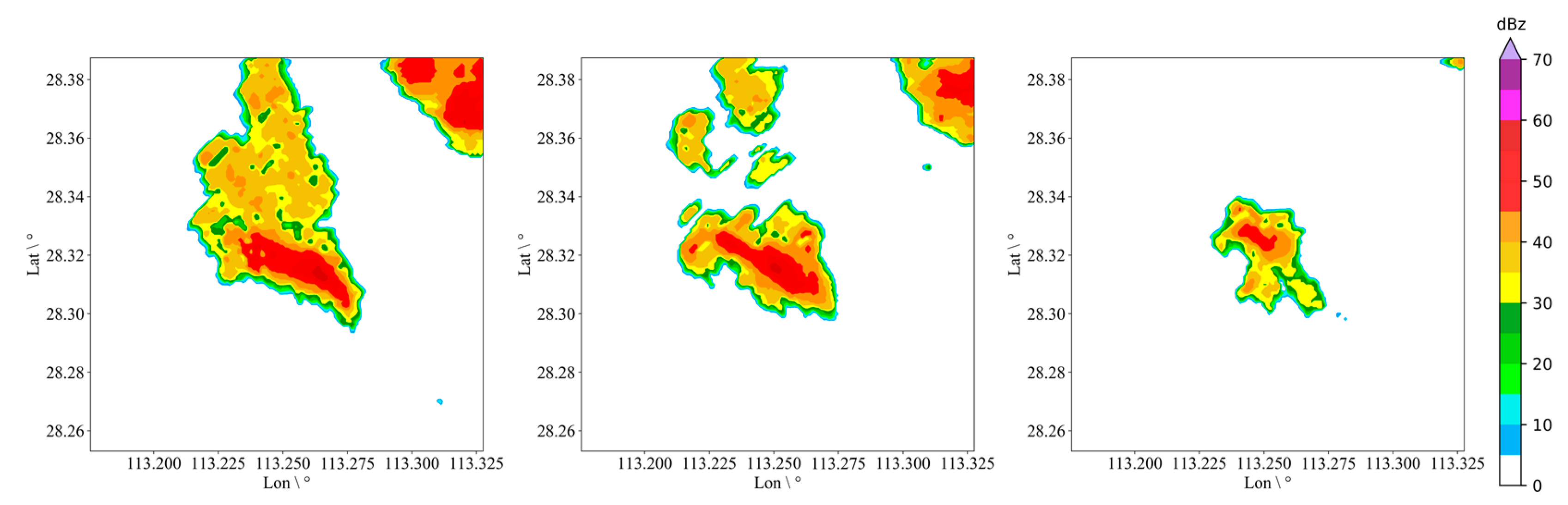
Figure 15 and Figure 16 show the fused high-resolution reflectivity in Constant Altitude Plan Position Indicator (CAPPI) display of reflectivity at different heights (1 km, 3 km, and 5 km) of the two commonly detected areas as indicated by the red and the blue circles in Figure 14. It can be seen that the fused high-resolution reflectivity at different heights present fine and complete echo structures.

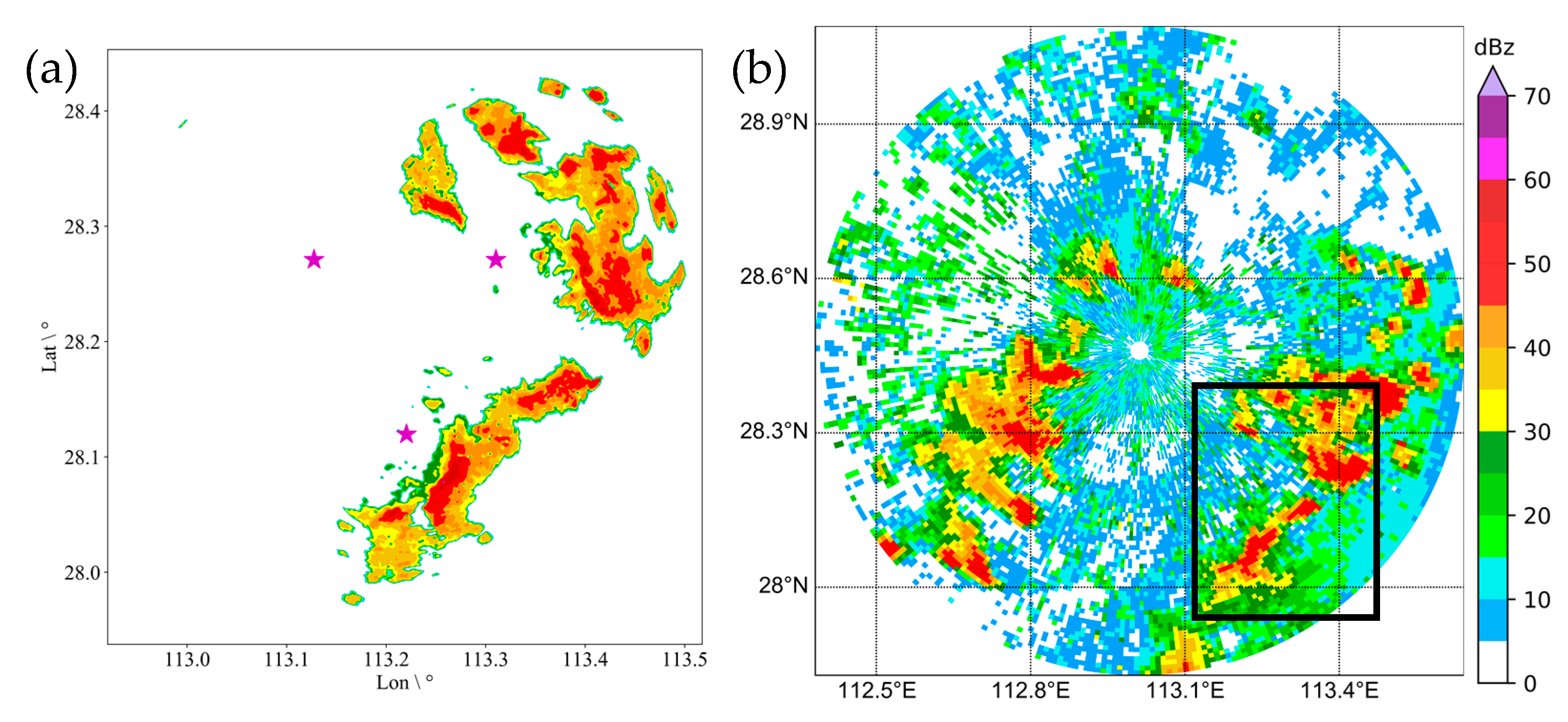
Fortunately, the precipitation event was also captured by the CINRAD radar in Changsha (113.01° E, 28.46° N), which provides another way of verifying the AWR fusion result. Figure 17 shows both AWR fused reflectivity at 1 km height (Figure 17a) valid at 05:49:12 UTC 15 August 2018 and the CINRAD radar PPI reflectivity at 0.6° elevation (Figure 17b) valid at 05:51:17 UTC 15 August 2018. Note that the AWR observation in Figure 17a corresponds to the black-box area in CINRAD radar observation in Figure 17b. There are several areas of strong echoes in the observation area. The strong reflectivity values are mainly in the range of 50–60 dBZ. The comparison suggests good consistency between the two radars. In addition, the details of the echoes captured by the AWR are abundant, which also validates the performance of the fusion process.

5. Discussions and Conclusions

Aiming at the demand for fine detection of small-scale weather systems, and based on the fine spatiotemporal resolution detection data of the new AWR, the high-resolution reflectivity fusion method for the new AWR is proposed in this paper. In the fine detection area of the AWR, the time difference of the obtained data from the three subarrays is about 2 s because of the rapid scanning mode of phased-array subarrays. The high-resolution reflectivity fusion method is based on the fact that the constant high range resolution compensates the azimuth and elevation resolutions of the AWR.

The performance of the fused high-resolution reflectivity is evaluated both subjectively and objectively using two simulated subarray scan experiments on a simulated heavy precipitation and a simulated tornado case. In comparison to the simulated ‘truth’ echoes, the subjective evaluation proves that the low azimuth resolution of one subarray can be enhanced by the other subarrays. The fusion of multiple subarray observation leads to the improved resolution, while finer and more complete radar echo structures can be obtained. By comparing to the ‘truth’ data in the objective evaluations with CC and RMSE, it is verified that the fused high-resolution reflectivity can reduce the detection deviation of each individual subarray.

Moreover, the high-resolution reflectivity fusion method is employed in a real precipitation event near Changsha Huanghua International Airport at 05:49:12 UTC 15 August 2018. It is proved that the AWR can capture the finer and more detailed echo structures of the severe precipitation than the CINRAD radar observation.

The AWR is a new instrument and there are inevitably some unrecognized issues. The case data that are available for high-resolution fusion only permitted two-subarray data fusion. With further observations being carried out, three or more subarray fusion will be possible and further testing of the resolution enhancement and fusion may provide more robust conclusions. Due to location of this real precipitation event, no quantitative comparison has been completed with the automatic weather station, which is also a future research direction.