
Tutorial: Guidelines for Single-Cell RT-qPCR


Abstract
1. Introduction
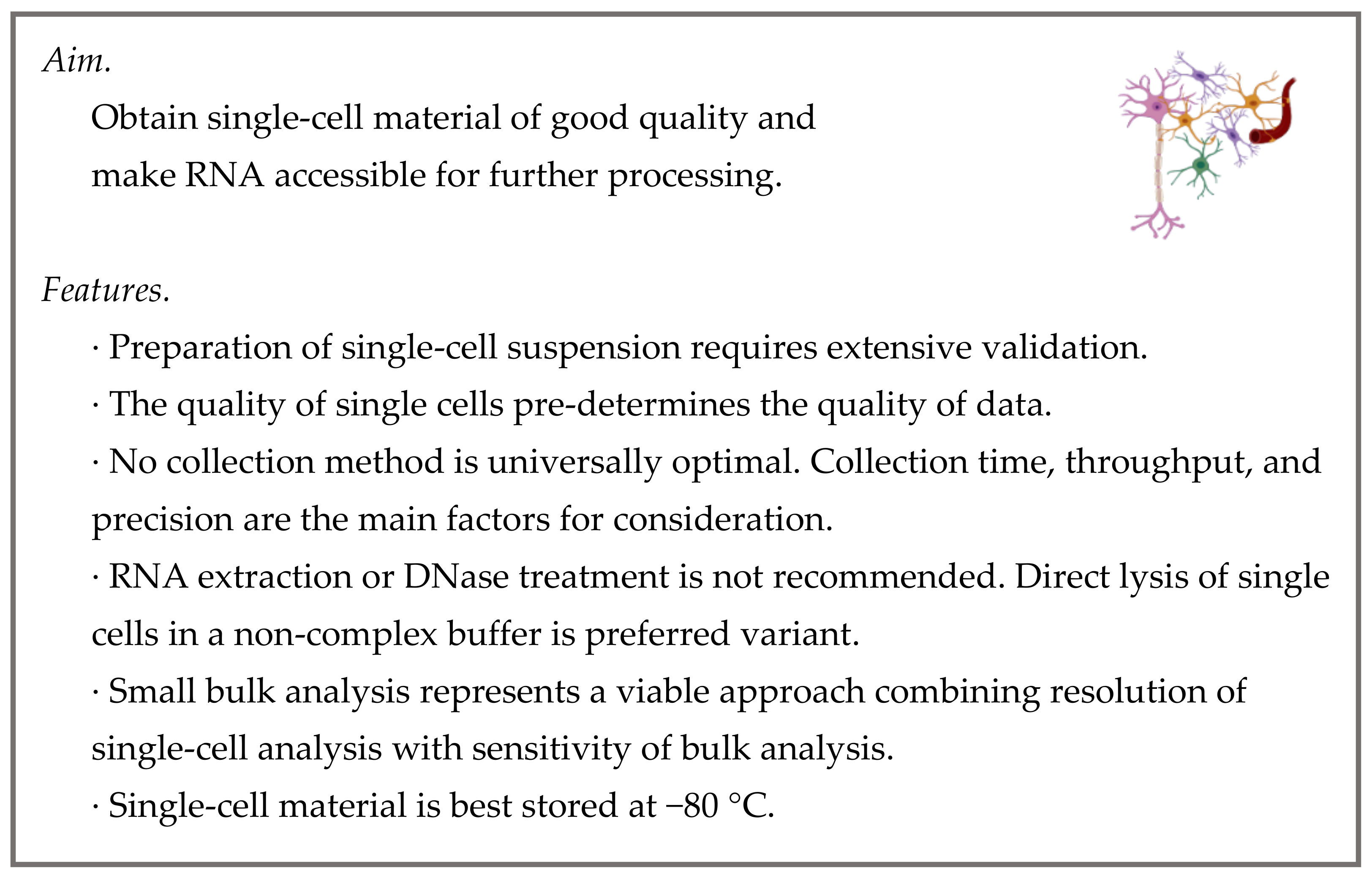
2. Sample collection
2.1. Preparation of Single-Cell Suspension
2.2. Single-Cell Collection
2.3. RNA Extraction and DNase Treatment
2.4. Direct Lysis
2.5. Storage Conditions
2.6. Small Bulk Analysis
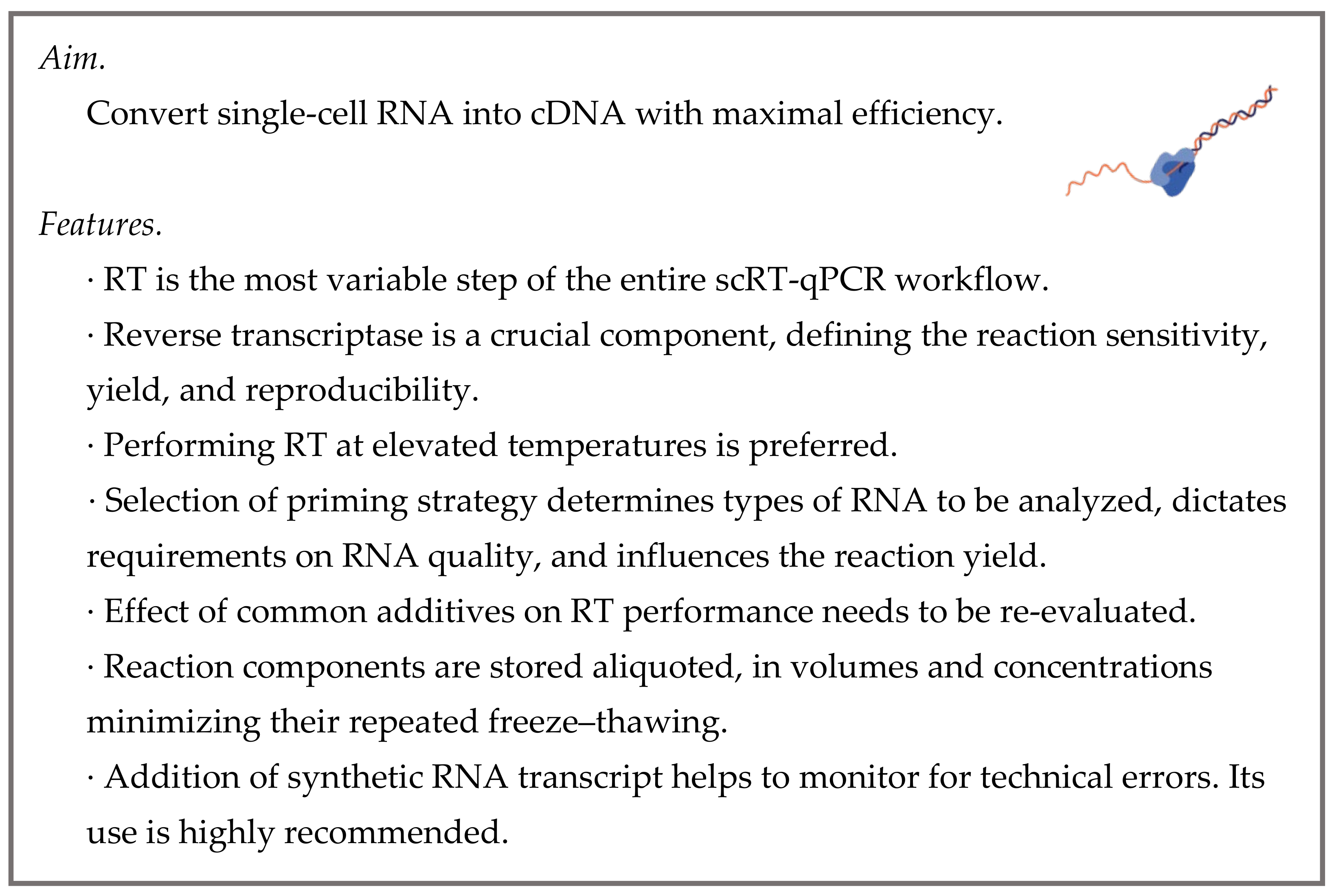
3. Reverse Transcription
3.1. RT-Associated Variables
3.2. RTase Selection
3.3. Priming Strategy
3.4. RT Additives
3.5. Temperature Profile
3.6. Setting RT Reaction
3.7. Quality Control
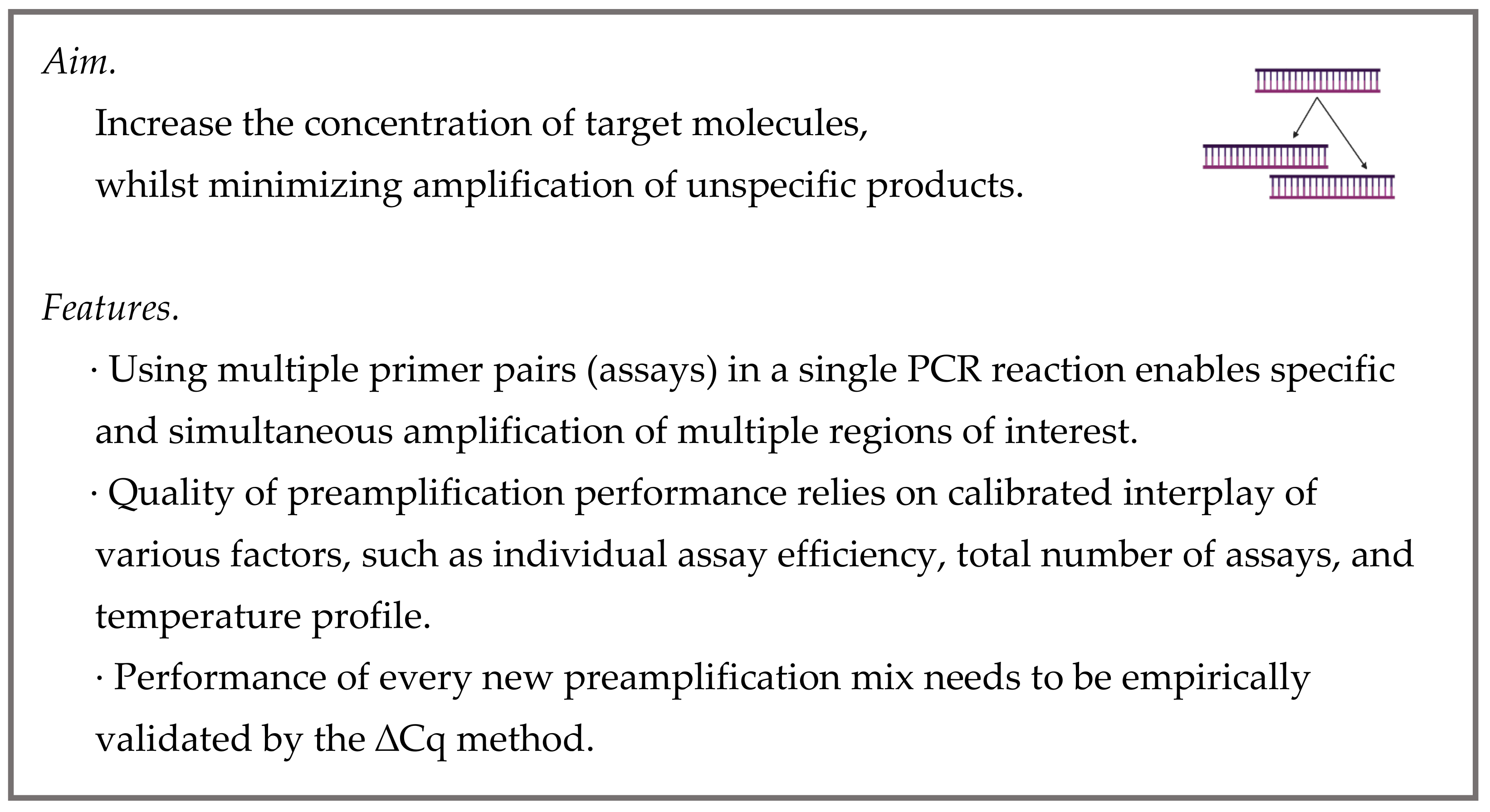
4. Preamplification
4.1. Targeted vs. Global Preamplification
4.2. Reaction Parameters
4.3. Validation
4.4. Setting preAMP Reaction
5. Quantitative PCR
5.1. Assay Design
5.2. Assay Validation
5.3. Limit of Detection and Limit of Quantification
5.4. Setting the qPCR Reaction
5.5. Quality Control
6. Data Analysis
6.1. Single-Cell Data Specifications
6.2. Data Pre-Processing
6.3. Descriptive Analysis and Data Visualization
7. Conclusions
Supplementary Materials
Funding
Institutional Review Board Statement
Informed Consent Statement
Data Availability Statement
Acknowledgments
Conflicts of Interest
Abbreviations
References
- Swarup, V.; Hinz, F.I.; Rexach, J.E.; Noguchi, K.; Toyoshiba, H.; Oda, A.; Hirai, K.; Sarkar, A.; Seyfried, N.T.; Cheng, C.; et al. Identification of evolutionarily conserved gene networks mediating neurodegenerative dementia. Nat. Med. 2019, 25, 152–164. [Google Scholar] [CrossRef] [PubMed]
- Maniatis, S.; Äijö, T.; Vickovic, S.; Braine, C.; Kang, K.; Mollbrink, A.; Fagegaltier, D.; Andrusivová, Ž.; Saarenpää, S.; Saiz-Castro, G.; et al. Spatiotemporal dynamics of molecular pathology in amyotrophic lateral sclerosis. Science 2019, 364, 89–93. [Google Scholar] [CrossRef] [PubMed]
- Kelley, K.W.; Nakao-Inoue, H.; Molofsky, A.V.; Oldham, M.C. Variation among intact tissue samples reveals the core transcriptional features of human CNS cell classes. Nat. Neurosci. 2018, 21, 1171–1184. [Google Scholar] [CrossRef] [PubMed]
- Habib, N.; McCabe, C.; Medina, S.; Varshavsky, M.; Kitsberg, D.; Dvir-Szternfeld, R.; Green, G.; Dionne, D.; Nguyen, L.; Marshall, J.L.; et al. Disease-associated astrocytes in Alzheimer’s disease and aging. Nat. Neurosci. 2020, 23, 701–706. [Google Scholar] [CrossRef] [PubMed]
- Mathys, H.; Davila-Velderrain, J.; Peng, Z.; Gao, F.; Mohammadi, S.; Young, J.Z.; Menon, M.; He, L.; Abdurrob, F.; Jiang, X.; et al. Single-cell transcriptomic analysis of Alzheimer’s disease. Nature 2019, 570, 332–337. [Google Scholar] [CrossRef] [PubMed]
- Sala Frigerio, C.; Wolfs, L.; Fattorelli, N.; Thrupp, N.; Voytyuk, I.; Schmidt, I.; Mancuso, R.; Chen, W.T.; Woodbury, M.E.; Srivastava, G.; et al. The Major Risk Factors for Alzheimer’s Disease: Age, Sex, and Genes Modulate the Microglia Response to Aβ Plaques. Cell Rep. 2019, 27, 1293–1306. [Google Scholar] [CrossRef]
- Liddelow, S.A.; Guttenplan, K.A.; Clarke, L.E.; Bennett, F.C.; Bohlen, C.J.; Schirmer, L.; Bennett, M.L.; Münch, A.E.; Chung, W.S.; Peterson, T.C.; et al. Neurotoxic reactive astrocytes are induced by activated microglia. Nature 2017, 541, 481–487. [Google Scholar] [CrossRef]
- Guttenplan, K.A.; Stafford, B.K.; El-Danaf, R.N.; Adler, D.I.; Münch, A.E.; Weigel, M.K.; Huberman, A.D.; Liddelow, S.A. Neurotoxic Reactive Astrocytes Drive Neuronal Death after Retinal Injury. Cell Rep. 2020, 31, 107776. [Google Scholar] [CrossRef]
- Keren-Shaul, H.; Spinrad, A.; Weiner, A.; Matcovitch-Natan, O.; Dvir-Szternfeld, R.; Ulland, T.K.; David, E.; Baruch, K.; Lara-Astaiso, D.; Toth, B.; et al. A Unique Microglia Type Associated with Restricting Development of Alzheimer’s Disease. Cell 2017, 169, 1276–1290. [Google Scholar] [CrossRef]
- Willis, E.F.; Macdonald, K.P.A.; Nguyen, Q.H.; Rose-John, S.; Ruitenberg, M.J.; Correspondence, J.V. Repopulating Microglia Promote Brain Repair in an IL-6-Dependent Manner. Cell 2020, 180, 833–846. [Google Scholar] [CrossRef]
- Wheeler, M.A.; Clark, I.C.; Tjon, E.C.; Li, Z.; Zandee, S.E.J.; Couturier, C.P.; Watson, B.R.; Scalisi, G.; Alkwai, S.; Rothhammer, V.; et al. MAFG-driven astrocytes promote CNS inflammation. Nature 2020, 578, 593. [Google Scholar] [CrossRef] [PubMed]
- Friedman, B.A.; Srinivasan, K.; Ayalon, G.; Meilandt, W.J.; Lin, H.; Huntley, M.A.; Cao, Y.; Lee, S.H.; Haddick, P.C.G.; Ngu, H.; et al. Diverse Brain Myeloid Expression Profiles Reveal Distinct Microglial Activation States and Aspects of Alzheimer’s Disease Not Evident in Mouse Models. Cell Rep. 2018, 22, 832–847. [Google Scholar] [CrossRef] [PubMed]
- Andersson, A.; Bergenstråhle, J.; Asp, M.; Bergenstråhle, L.; Jurek, A.; Fernández Navarro, J.; Lundeberg, J. Single-cell and spatial transcriptomics enables probabilistic inference of cell type topography. Commun. Biol. 2020, 3, 1–8. [Google Scholar] [CrossRef] [PubMed]
- Chung, W.; Eum, H.H.; Lee, H.O.; Lee, K.M.; Lee, H.B.; Kim, K.T.; Ryu, H.S.; Kim, S.; Lee, J.E.; Park, Y.H.; et al. Single-cell RNA-seq enables comprehensive tumour and immune cell profiling in primary breast cancer. Nat. Commun. 2017, 8, 1–12. [Google Scholar] [CrossRef]
- Milich, L.M.; Choi, J.S.; Ryan, C.; Cerqueira, S.R.; Benavides, S.; Yahn, S.L.; Tsoulfas, P.; Lee, J.K. Single-cell analysis of the cellular heterogeneity and interactions in the injured mouse spinal cord. J. Exp. Med. 2021, 218, 1–25. [Google Scholar] [CrossRef]
- Bayraktar, O.A.; Bartels, T.; Holmqvist, S.; Kleshchevnikov, V.; Martirosyan, A.; Polioudakis, D.; Ben Haim, L.; Young, A.M.H.; Batiuk, M.Y.; Prakash, K.; et al. Astrocyte layers in the mammalian cerebral cortex revealed by a single-cell in situ transcriptomic map. Nat. Neurosci. 2020, 23, 500–509. [Google Scholar] [CrossRef]
- Ståhlberg, A.; Thomsen, C.; Ruff, D.; Åman, P. Quantitative PCR Analysis of DNA, RNAs, and Proteins in the Same Single Cell. Clin. Chem. 2012, 58, 1682–1691. [Google Scholar] [CrossRef]
- Bustin, S.A.; Mueller, R. Real-time reverse transcription PCR (qRT-PCR) and its potential use in clinical diagnosis. Clin. Sci. 2005, 109, 365–379. [Google Scholar] [CrossRef]
- Kubista, M.; Andrade, J.M.; Bengtsson, M.; Forootan, A.; Jonák, J.; Lind, K.; Sindelka, R.; Sjöback, R.; Sjögreen, B.; Strömbom, L.; et al. The real-time polymerase chain reaction. Mol. Aspects Med. 2006, 27, 95–125. [Google Scholar] [CrossRef]
- Tichopad, A.; Kitchen, R.; Riedmaier, I.; Becker, C.; Ståhlberg, A.; Kubista, M. Design and optimization of reverse-transcription quantitative PCR experiments. Clin. Chem. 2009, 55, 1816–1823. [Google Scholar] [CrossRef]
- Bar, T.; Kubista, M.; Tichopad, A. Validation of kinetics similarity in qPCR. Nucleic Acids Res. 2012, 40, 1395–1406. [Google Scholar] [CrossRef]
- Ståhlberg, A.; Kubista, M. The workflow of single-cell expression profiling using quantitative real-time PCR. Expert Rev. Mol. Diagn. 2014, 14, 323–331. [Google Scholar] [CrossRef] [PubMed]
- Ståhlberg, A.; Kubista, M. Technical aspects and recommendations for single-cell qPCR. Mol. Aspects Med. 2018, 59, 28–35. [Google Scholar] [CrossRef] [PubMed]
- Svec, D.; Tichopad, A.; Novosadova, V.; Pfaffl, M.W.; Kubista, M. How good is a PCR efficiency estimate: Recommendations for precise and robust qPCR efficiency assessments. Biomol. Detect. Quantif. 2015, 3, 9–16. [Google Scholar] [CrossRef]
- Bustin, S.; Huggett, J. qPCR primer design revisited. Biomol. Detect. Quantif. 2017, 14, 19–28. [Google Scholar] [CrossRef]
- Ståhlberg, A.; Kubista, M.; Åman, P. Single-cell gene-expression profiling and its potential diagnostic applications. Expert Rev. Mol. Diagn. 2011, 11, 735–740. [Google Scholar] [CrossRef][Green Version]
- Ståhlberg, A.; Bengtsson, M. Single-cell gene expression profiling using reverse transcription quantitative real-time PCR. Methods 2010, 50, 282–288. [Google Scholar] [CrossRef]
- Ståhlberg, A.; Rusnakova, V.; Kubista, M. The added value of single-cell gene expression profiling. Brief. Funct. Genom. 2013, 12, 81–89. [Google Scholar] [CrossRef]
- Lafzi, A.; Moutinho, C.; Picelli, S.; Heyn, H. Tutorial: Guidelines for the experimental design of single-cell RNA sequencing studies. Nat. Protoc. 2018, 13, 2742–2757. [Google Scholar] [CrossRef]
- Andrews, T.S.; Kiselev, V.Y.; McCarthy, D.; Hemberg, M. Tutorial: Guidelines for the computational analysis of single-cell RNA sequencing data. Nat. Protoc. 2021, 16, 1–9. [Google Scholar] [CrossRef] [PubMed]
- van den Brink, S.C.; Sage, F.; Vértesy, Á.; Spanjaard, B.; Peterson-Maduro, J.; Baron, C.S.; Robin, C.; van Oudenaarden, A. Single-cell sequencing reveals dissociation-induced gene expression in tissue subpopulations. Nat. Methods 2017, 14, 935–936. [Google Scholar] [CrossRef]
- Marsh, S.E.; Kamath, T.; Walker, A.J.; Dissing-Olesen, L.; Hammond, T.R.; Young, A.M.H.; Abdulraouf, A.; Nadaf, N.; Dufort, C.; Murphy, S.; et al. Single Cell Sequencing Reveals Glial Specific Responses to Tissue Processing & Enzymatic Dissociation in Mice and Humans Single Cell Sequencing Reveals Glial Specific Responses to Tissue Processing & Enzymatic Dissociation in Mice and Humans. bioRxiv 2020, 1–13. [Google Scholar]
- Hodne, K.; Weltzien, F.-A. Single-Cell Isolation and Gene Analysis: Pitfalls and Possibilities. Int. J. Mol. Sci. 2015, 16, 26832–26849. [Google Scholar] [CrossRef]
- Abaffy, P.; Lettlova, S.; Truksa, J.; Kubista, M.; Sindelka, R. Preparation of single-cell suspension from mouse breast cancer focusing on preservation of original cell state information and cell type composition. bioRxiv 2019. [Google Scholar] [CrossRef]
- O’Flanagan, C.H.; Campbell, K.R.; Zhang, A.W.; Kabeer, F.; Lim, J.L.P.; Biele, J.; Eirew, P.; Lai, D.; McPherson, A.; Kong, E.; et al. Dissociation of solid tumor tissues with cold active protease for single-cell RNA-seq minimizes conserved collagenase-associated stress responses. Genome Biol. 2019, 20, 1–13. [Google Scholar] [CrossRef] [PubMed]
- Wu, Y.E.; Pan, L.; Zuo, Y.; Li, X.; Hong, W. Detecting Activated Cell Populations Using Single-Cell RNA-Seq. Neuron 2017, 96, 313–329. [Google Scholar] [CrossRef] [PubMed]
- Adam, M.; Potter, A.S.; Potter, S.S. Psychrophilic proteases dramatically reduce single-cell RNA-seq artifacts: A molecular atlas of kidney development. Development 2017, 144, 3625–3632. [Google Scholar] [CrossRef]
- Valihrach, L.; Androvic, P.; Kubista, M. Platforms for Single-Cell Collection and Analysis. Int. J. Mol. Sci. 2018, 19, 807. [Google Scholar] [CrossRef]
- Kuhn, A.; Kumar, A.; Beilina, A.; Dillman, A.; Cookson, M.R.; Singleton, A.B. Cell population-specific expression analysis of human cerebellum. BMC Genom. 2012, 13, 610. [Google Scholar] [CrossRef]
- Datta, S.; Malhotra, L.; Dickerson, R.; Chaffee, S.; Sen, C.K.; Roy, S. Laser capture microdissection: Big data from small samples. Histol. Histopathol. 2015, 30, 1255–1269. [Google Scholar]
- Adan, A.; Alizada, G.; Kiraz, Y.; Baran, Y.; Nalbant, A. Flow cytometry: Basic principles and applications. Crit. Rev. Biotechnol. 2017, 37, 163–176. [Google Scholar] [CrossRef] [PubMed]
- Tan, S.J.; Li, Q.; Lim, C.T. Manipulation and Isolation of Single Cells and Nuclei. Methods Cell Biol. 2010, 98, 79–96. [Google Scholar]
- Lee, L.M.; Liu, A.P. The application of micropipette aspiration in molecular mechanics of single cells. J. Nanotechnol. Eng. Med. 2015, 5. [Google Scholar] [CrossRef]
- Dzamba, D.; Valihrach, L.; Kubista, M.; Anderova, M. The correlation between expression profiles measured in single cells and in traditional bulk samples. Sci. Rep. 2016, 6, 37022. [Google Scholar] [CrossRef] [PubMed]
- Svec, D.; Andersson, D.; Pekny, M.; Sjöback, R.; Kubista, M.; Ståhlberg, A. Direct Cell Lysis for Single-Cell Gene Expression Profiling. Front. Oncol. 2013, 3, 274. [Google Scholar] [CrossRef] [PubMed]
- Wang, Y.; Zheng, H.; Chen, J.; Zhong, X.; Wang, Y.; Wang, Z.; Wang, Y. The Impact of Different Preservation Conditions and Freezing-Thawing Cycles on Quality of RNA, DNA, and Proteins in Cancer Tissue. Biopreserv. Biobank. 2015, 13, 335–347. [Google Scholar] [CrossRef]
- Ji, X.; Wang, M.; Li, L.; Chen, F.; Zhang, Y.; Li, Q.; Zhou, J. The Impact of Repeated Freeze-Thaw Cycles on the Quality of Biomolecules in Four Different Tissues. Biopreserv. Biobank. 2017, 15, 475–483. [Google Scholar] [CrossRef] [PubMed]
- Marinov, G.K.; Williams, B.A.; McCue, K.; Schroth, G.P.; Gertz, J.; Myers, R.M.; Wold, B.J. From single-cell to cell-pool transcriptomes: Stochasticity in gene expression and RNA splicing. Genome Res. 2014, 24, 496–510. [Google Scholar] [CrossRef]
- Kubista, M.; Dreyer-Lamm, J.; Ståhlberg, A. The secrets of the cell. Mol. Aspects Med. 2018, 59, 1–4. [Google Scholar] [CrossRef] [PubMed]
- Lindén, J.; Ranta, J.; Pohjanvirta, R. Bayesian modeling of reproducibility and robustness of RNA reverse transcription and quantitative real-time polymerase chain reaction. Anal. Biochem. 2012, 428, 81–91. [Google Scholar] [CrossRef] [PubMed]
- Sieber, M.W.; Recknagel, P.; Glaser, F.; Witte, O.W.; Bauer, M.; Claus, R.A.; Frahm, C. Substantial performance discrepancies among commercially available kits for reverse transcription quantitative polymerase chain reaction: A systematic comparative investigator-driven approach. Anal. Biochem. 2010, 401, 303–311. [Google Scholar] [CrossRef] [PubMed]
- Bustin, S.; Dhillon, H.S.; Kirvell, S.; Greenwood, C.; Parker, M.; Shipley, G.L.; Nolan, T. Variability of the reverse transcription step: Practical implications. Clin. Chem. 2015, 61, 202–212. [Google Scholar] [CrossRef]
- Ståhlberg, A.; Håkansson, J.; Xian, X.; Semb, H.; Kubista, M. Properties of the Reverse Transcription Reaction in mRNA Quantification. Clin. Chem. 2004, 50, 509–515. [Google Scholar] [CrossRef]
- Bengtsson, M.; Hemberg, M.; Rorsman, P.; Ståhlberg, A. Quantification of mRNA in single cells and modelling of RT-qPCR induced noise. BMC Mol. Biol. 2008, 9, 63. [Google Scholar] [CrossRef] [PubMed]
- Schwaber, J.; Andersen, S.; Nielsen, L. Shedding light: The importance of reverse transcription efficiency standards in data interpretation. Biomol. Detect. Quantif. 2019, 17, 100077. [Google Scholar] [CrossRef] [PubMed]
- Zucha, D.; Androvic, P.; Kubista, M.; Valihrach, L. Performance Comparison of Reverse Transcriptases for Single-Cell Studies. Clin. Chem. 2020, 66, 217–228. [Google Scholar] [CrossRef]
- Ståhlberg, A. Comparison of Reverse Transcriptases in Gene Expression Analysis. Clin. Chem. 2004, 50, 1678–1680. [Google Scholar] [CrossRef] [PubMed]
- Miranda, J.A.; Steward, G.F. Variables influencing the efficiency and interpretation of reverse transcription quantitative PCR (RT-qPCR): An empirical study using Bacteriophage MS2. J. Virol. Methods 2017, 241, 1–10. [Google Scholar] [CrossRef] [PubMed]
- Nardon, E.; Donada, M.; Bonin, S.; Dotti, I.; Stanta, G. Higher random oligo concentration improves reverse transcription yield of cDNA from bioptic tissues and quantitative RT-PCR reliability. Exp. Mol. Pathol. 2009, 87, 146–151. [Google Scholar] [CrossRef]
- Levesque-Sergerie, J.-P.; Duquette, M.; Thibault, C.; Delbecchi, L.; Bissonnette, N. Detection limits of several commercial reverse transcriptase enzymes: Impact on the low- and high-abundance transcript levels assessed by quantitative RT-PCR. BMC Mol. Biol. 2007, 8, 93. [Google Scholar] [CrossRef]
- Bagnoli, J.W.; Ziegenhain, C.; Janjic, A.; Wange, L.E.; Vieth, B.; Parekh, S.; Geuder, J.; Hellmann, I.; Enard, W. Sensitive and powerful single-cell RNA sequencing using mcSCRB-seq. Nat. Commun. 2018, 9, 2937. [Google Scholar] [CrossRef]
- Skirgaila, R.; Pudzaitis, V.; Paliksa, S.; Vaitkevicius, M.; Janulaitis, A. Compartmentalization of destabilized enzyme-mRNA-ribosome complexes generated by ribosome display: A novel tool for the directed evolution of enzymes. Protein Eng. Des. Sel. 2013, 26, 453–461. [Google Scholar] [CrossRef][Green Version]
- Mohr, S.; Ghanem, E.; Smith, W.; Sheeter, D.; Qin, Y.; King, O.; Polioudakis, D.; Iyer, V.R.; Hunicke-Smith, S.; Swamy, S.; et al. Thermostable group II intron reverse transcriptase fusion proteins and their use in cDNA synthesis and next-generation RNA sequencing. Rna 2013, 19, 958–970. [Google Scholar] [CrossRef] [PubMed]
- Arezi, B.; Hogrefe, H. Novel mutations in Moloney Murine Leukemia Virus reverse transcriptase increase thermostability through tighter binding to template-primer. Nucleic Acids Res. 2009, 37, 473–481. [Google Scholar] [CrossRef] [PubMed]
- Nolan, T.; Hands, R.E.; Bustin, S.A. Quantification of mRNA using real-time RT-PCR. Nat. Protoc. 2006, 1, 1559–1582. [Google Scholar] [CrossRef] [PubMed]
- Álvarez, M.; Menéndez-Arias, L. Temperature effects on the fidelity of a thermostable HIV-1 reverse transcriptase. FEBS J. 2014, 281, 342–351. [Google Scholar] [CrossRef] [PubMed]
- Forootan, A.; Sjöback, R.; Björkman, J.; Sjögreen, B.; Linz, L.; Kubista, M. Methods to determine limit of detection and limit of quantification in quantitative real-time PCR (qPCR). Biomol. Detect. Quantif. 2017, 12, 1–6. [Google Scholar] [CrossRef] [PubMed]
- Svensson, V.; Natarajan, K.N.; Ly, L.-H.; Miragaia, R.J.; Labalette, C.; Macaulay, I.C.; Cvejic, A.; Teichmann, S.A. Power analysis of single-cell RNA-sequencing experiments. Nat. Methods 2017, 14, 381–387. [Google Scholar] [CrossRef]
- Baranauskas, A.; Paliksa, S.; Alzbutas, G.; Vaitkevicius, M.; Lubiene, J.; Letukiene, V.; Burinskas, S.; Sasnauskas, G.; Skirgaila, R. Generation and characterization of new highly thermostable and processive M-MuLV reverse transcriptase variants. Protein Eng. Des. Sel. 2012, 25, 657–668. [Google Scholar] [CrossRef]
- Ziegenhain, C.; Vieth, B.; Parekh, S.; Reinius, B.; Guillaumet-Adkins, A.; Smets, M.; Leonhardt, H.; Heyn, H.; Hellmann, I.; Enard, W. Comparative Analysis of Single-Cell RNA Sequencing Methods. Mol. Cell 2017, 65, 631–643. [Google Scholar] [CrossRef] [PubMed]
- Bustin, S.A.; Nolan, T. Pitfalls of quantitative real- time reverse-transcription polymerase chain reaction. J. Biomol. Tech. 2004, 15, 155–166. [Google Scholar] [PubMed]
- Picelli, S.; Faridani, O.R.; Björklund, A.K.; Winberg, G.; Sagasser, S.; Sandberg, R. Full-length RNA-seq from single cells using Smart-seq2. Nat. Protoc. 2014, 9, 171–181. [Google Scholar] [CrossRef] [PubMed]
- Attwater, J.; Wochner, A.; Pinheiro, V.B.; Coulson, A.; Holliger, P. Ice as a protocellular medium for RNA replication. Nat. Commun. 2010, 1, 1–9. [Google Scholar] [CrossRef]
- Aicher, T.P.; Carroll, S.; Raddi, G.; Gierahn, T.; Wadsworth, M.H.; Hughes, T.K.; Love, C.; Shalek, A.K. Seq-Well: A sample-efficient, portable picowell platform for massively parallel single-cell RNA sequencing. Methods Mol. Biol. 2019, 1979, 111–132. [Google Scholar] [PubMed]
- Hashimshony, T.; Senderovich, N.; Avital, G.; Klochendler, A.; de Leeuw, Y.; Anavy, L.; Gennert, D.; Li, S.; Livak, K.J.; Rozenblatt-Rosen, O.; et al. CEL-Seq2: Sensitive highly-multiplexed single-cell RNA-Seq. Genome Biol. 2016, 17, 1–7. [Google Scholar] [CrossRef]
- Nolan, T.; Hands, R.E.; Ogunkolade, W.; Bustin, S.A. SPUD: A quantitative PCR assay for the detection of inhibitors in nucleic acid preparations. Anal. Biochem. 2006, 351, 308–310. [Google Scholar] [CrossRef]
- External RNA Controls Consortium Proposed methods for testing and selecting the ERCC external RNA controls. BMC Genomics 2005, 6, 150. [CrossRef]
- Livak, K.J.; Wills, Q.F.; Tipping, A.J.; Datta, K.; Mittal, R.; Goldson, A.J.; Sexton, D.W.; Holmes, C.C. Methods for qPCR gene expression profiling applied to 1440 lymphoblastoid single cells. Methods 2013, 59, 71–79. [Google Scholar] [CrossRef]
- Andersson, D.; Akrap, N.; Svec, D.; Godfrey, T.E.; Kubista, M.; Landberg, G.; Ståhlberg, A. Properties of targeted preamplification in DNA and cDNA quantification. Expert Rev. Mol. Diagn. 2015, 15, 1085–1100. [Google Scholar] [CrossRef]
- Kroneis, T.; Jonasson, E.; Andersson, D.; Dolatabadi, S.; Ståhlberg, A. Global preamplification simplifies targeted mRNA quantification. Sci. Rep. 2017, 7, 45219. [Google Scholar] [CrossRef]
- Korenková, V.; Scott, J.; Novosadová, V.; Jindřichová, M.; Langerová, L.; Švec, D.; Šídová, M.; Sjöback, R. Pre-amplification in the context of high-throughput qPCR gene expression experiment. BMC Mol. Biol. 2015, 16, 5. [Google Scholar] [CrossRef] [PubMed]
- Laurell, H.; Iacovoni, J.S.; Abot, A.; Svec, D.; Maoret, J.J.; Arnal, J.F.; Kubista, M. Correction of RT-qPCR data for genomic DNA-derived signals with ValidPrime. Nucleic Acids Res. 2012, 40, e51. [Google Scholar] [CrossRef] [PubMed]
- Okello, J.B.A.; Rodriguez, L.; Poinar, D.; Bos, K.; Okwi, A.L.; Bimenya, G.S.; Sewankambo, N.K.; Henry, K.R.; Kuch, M.; Poinar, H.N. Quantitative assessment of the sensitivity of various commercial reverse transcriptases based on armored HIV RNA. PLoS ONE 2010, 5, e13931. [Google Scholar] [CrossRef] [PubMed]
- Suslov, O.; Steindler, D.A. PCR inhibition by reverse transcriptase leads to an overestimation of amplification efficiency. Nucleic Acids Res. 2005, 33, 1–12. [Google Scholar] [CrossRef] [PubMed]
- Ye, J.; Coulouris, G.; Zaretskaya, I.; Cutcutache, I.; Rozen, S.; Madden, T.L. Primer-BLAST: A tool to design target-specific primers for polymerase chain reaction. BMC Bioinform. 2012, 13, 134. [Google Scholar] [CrossRef]
- Burns, M.; Valdivia, H. Modelling the limit of detection in real-time quantitative PCR. Eur. Food Res. Technol. 2008, 226, 1513–1524. [Google Scholar] [CrossRef]
- Ståhlberg, A.; Rusnakova, V.; Forootan, A.; Anderova, M.; Kubista, M. RT-qPCR work-flow for single-cell data analysis. Methods 2013, 59, 80–88. [Google Scholar] [CrossRef]
- Bergkvist, A.; Rusnakova, V.; Sindelka, R.; Garda, J.M.A.; Sjögreen, B.; Lindh, D.; Forootan, A.; Kubista, M. Gene expression profiling—Clusters of possibilities. Methods 2010, 50, 323–335. [Google Scholar] [CrossRef]
- Riedmaier, I.; Pfaffl, M.W. Transcriptional biomarkers—High throughput screening, quantitative verification, and bioinformatical validation methods. Methods 2013, 59, 3–9. [Google Scholar] [CrossRef]


Publisher’s Note: MDPI stays neutral with regard to jurisdictional claims in published maps and institutional affiliations. |
© 2021 by the authors. Licensee MDPI, Basel, Switzerland. This article is an open access article distributed under the terms and conditions of the Creative Commons Attribution (CC BY) license (https://creativecommons.org/licenses/by/4.0/).
Share and Cite
Zucha, D.; Kubista, M.; Valihrach, L. Tutorial: Guidelines for Single-Cell RT-qPCR. Cells 2021, 10, 2607. https://doi.org/10.3390/cells10102607
Zucha D, Kubista M, Valihrach L. Tutorial: Guidelines for Single-Cell RT-qPCR. Cells. 2021; 10(10):2607. https://doi.org/10.3390/cells10102607
Chicago/Turabian StyleZucha, Daniel, Mikael Kubista, and Lukas Valihrach. 2021. "Tutorial: Guidelines for Single-Cell RT-qPCR" Cells 10, no. 10: 2607. https://doi.org/10.3390/cells10102607
APA StyleZucha, D., Kubista, M., & Valihrach, L. (2021). Tutorial: Guidelines for Single-Cell RT-qPCR. Cells, 10(10), 2607. https://doi.org/10.3390/cells10102607