Article

Field Spectroscopy: A Non-Destructive Technique for Estimating Water Status in Vineyards

by
Ana Belén González-Fernández
1,
Enoc Sanz-Ablanedo
1,
Víctor Marcelo Gabella
2,
Marta García-Fernández
1 and
José Ramón Rodríguez-Pérez
1,*
1
Grupo de Investigación en Geomática e Ingeniería Cartográfica (GEOINCA), Universidad de León, Avenida de Astorga sn, 24401 Ponferrada, León, Spain
2
Departamento de Ingeniería y Ciencias Agrarias, Universidad de León, Av. Astorga s/n, 24401 Ponferrada, León, Spain
*
Author to whom correspondence should be addressed.
Agronomy 2019, 9(8), 427; https://doi.org/10.3390/agronomy9080427
Submission received: 20 May 2019 / Revised: 16 July 2019 / Accepted: 31 July 2019 / Published: 3 August 2019

Abstract

:
Water status controls plant physiology and is key to managing vineyard grape quality and yield. Water status is usually estimated by leaf water potential (LWP), which is measured using a pressure chamber; however, this method is difficult, time-consuming, and error-prone. While traditional spectral methods based on leaf reflectance are faster and non-destructive, most are based on vegetation indices derived from satellite imagery (and so only take into account discrete bandwidths) and do not take full advantage of modern hyperspectral sensors that capture spectral reflectance for thousands of wavelengths. We used partial least squares regression (PLSR) to predict LWP from reflectance values (wavelength 350–2500 nm) captured with a field spectroradiometer. We first identified wavelength ranges that minimized regression error. We then tested several common data pre-processing methods to analyze the impact on PLSR prediction precision, finding that derivative pre-processing increased the determination coefficients of our models and reduced root mean squared error (RMSE). The models fitted with raw data obtained their best results at around 1450 nm, while the models with derivative pre-processed achieved their best estimates at 826 nm and 1520 nm.

1. Introduction

Proper vine development depends on water availability, which affects plant physiology and, therefore, yield and grape composition. Irrigation scheduling is crucial because water deficiency negatively affects plant growth by modifying leaf pigment composition, reducing content in biochemical elements, and affecting turgor and cell enlargement [1]. In water stress conditions, photosynthesis slows down and metabolism is affected by alterations in the transport and uptake of nutrients, retarding plant growth [2] and sometimes even resulting in vine death.
Several methods can be used to estimate water status in crops. In viticulture, the main method is measurement of leaf water potential (LWP) [3], which requires measuring sap pressure in the xylem [4] using a pressure chamber. In California’s San Joaquin Valley vineyards, the water status of vines was measured using a pressure chamber combined with near-infrared techniques [5]. Other authors used a pressure chamber to estimate vine water status, concluding that vine water content is a key factor in final berry mass [6]. However, although measuring leaf pressure provides the most accurate assessment of plant water status, this method is destructive, slow, and laborious for estimating water content [7] and is not suitable for estimates involving large areas [5]. Moreover, the results may be influenced by temperature, light, size, and leaf position [8].
The Scholander pressure chamber has been widely used as the best method to estimate plant water status (specifically water potential). However, as an alternative to this destructive method, in recent years, novel methods have become available that allow less intrusive estimates of plant water status. Since the physiological electrical property of plants is related to water content [9] (in fact, the electrical behaviour of a plant is relatively resistive, as the tissue contains water [10]), several systems have used this property to estimate plant water status (and especially relative water content). This technique was successfully tested in plants such as Labisia pumila [11], Camellia sinensis [12], Solanum lycopersicum [13], and Lactuca sativa [14]. Recently, systems have been developed that allow continuous monitoring of water status in plants. Information is transmitted wirelessly and recorded by a data logger to conduct real-time assessment and remote regulation of irrigation. The leaf patch-clamp pressure probe is a non-invasive, accurate, and low-cost solution that is based on monitoring cell turgor pressure changes [15,16]. The new methods, based on recent technological advances, allow water plant status to be assessed online in real-time. While microwaves could enable estimation of water status in the field, this approach is influenced by leaf size [17]. Other methods based on broadband ultrasonic spectroscopy [18] and S-band reflectivity can be used as remote water status assessment techniques for Vitis vinifera L [19]. These non-invasive and non-contact techniques allow repeated measurements for water status monitoring.
Some studies determined that water content could be estimated by remote sensing, which would detect variations in plant reflectance, especially by leaves [20,21], or demonstrated that estimating water content using spectral data was more effective than the pressure chamber method [5]. A further study used spectral data to relate water content with vine vigour [22].
Some authors used vegetation indices, calculated from spectral values derived from satellite imagery, to estimate water content in vines, which required just two bands [8]. Vine water status estimated at both the leaf and canopy levels showed a strong relationship between the water index (ratio of reflectance at 900 nm and 970 nm) and stomatal conductance (gs) and between the normalized difference vegetation index (ratio of the difference between infrared and red reflectance and the sum of infrared and red reflectance) and predawn LWP [8].
However, hyperspectral datasets contain useful information for characterizing vegetation that is not represented using narrow-band indices, which only take into account a small part of the spectral data. Statistical methods, such as partial least squares regression (PLSR)—a statistical method similar to principal component regression—allow wide ranges of spectral data to be used to estimate water content. PLSR transforms the spectral feature space to obtain latent factors for a model with maximum variance in the feature space [23]. The main difference between PLSR and principal component regression is that, while principal component regression decomposes the spectra into a set of eigenvectors and scores and then regresses them against the response variables, PLRS uses response variable information during the decomposition process [24]. PSLR suitability for estimating water leaf content has been corroborated by authors who have estimated vine leaf water content [25] and water content and biochemical parameters [26,27,28].
Although these studies demonstrate the connection between spectral response and plant water status, spectral measurements are influenced by external factors, such as the inclination angle of the sun, surface roughness, the position of the fibre optic cable of the sensor, etc. One way to avoid these problems in collecting data is to use a spectroradiometer with a plant probe accessory [29] that stabilizes incident angle and light intensity.
Spectral data contain a mix of diffuse and specular reflectance for three main reasons: (i) Particle size, (ii) scatter, and (iii) multi-collinearity [30]. Differences in particle size in the material causes light to be deviated at different angles depending on the wavelength. Scattering effects, along with possible differences in path length, are the major cause of near-infrared variations. Scattering effects can be both additive and multiplicative. Additive effects produce a baseline displacement of the spectrum along the vertical axis, while multiplicative effects modify the local slope of the spectrum. Multiplicative combinations of these effects are the major factor inhibiting the interpretation of near-infrared diffuse reflectance spectra [30]. To minimize these effects, pre-processing spectral data may improve prediction models, enhancing the signal-to-noise ratio and the accuracy of the prediction models [31]. A well-designed pre-processing step will greatly improve model performance and avoid multi-collinearity. Derivative transformation [32,33] is typically used to smooth spectral data so as to improve the relationship between dependent and independent variables.
One way to minimize the problems associated with the external factors described above and with diffuse and specular reflectance is to use normalization tools. Normalization consists of a set of transformations whose purpose is to standardize the spectral signatures so that all data are at a similar scale. Several normalization methods exist, as described by CAMO Software AS [34]. Moreover, several spectral transformations can be used to mitigate spectral noise and diffuse and specular reflectance, including standard normal variate (SNV), multiplicative scatter correction (MSC), de-trending, and continuum removal (CR).
SNV is a pre-processing method that can be applied to each spectrum individually to remove scatter. SNV calculates the average and standard deviation values of all the data points for a given spectrum, obtaining the mean value for absorbance for each data point and dividing the result by the standard deviation [35]. Previous research found that, in using SNV, the diffuse reflectance spectra was free from multi-collinearity and there was no confusion from the complexity of shapes encountered in derivative spectroscopy [30]. MSC minimizes additive and multiplicative effects in spectral data by eliminating optical interference [36], removing physical effects produced by particle size and surface blaze from the spectra. MSC assumes that each spectrum is determined by sample characteristics and by particle size. Particle size can be represented by a baseline effect and the trend by means of a standard spectrum. MSC corrects the differences in the baseline and trend so that the transformed spectra are similar to the original spectra. Studies suggest that when MSC is used for data pre-processing, the coefficients obtained are robust for online prediction of material properties [36]. De-trending removes curvilinearity and baseline shift, improving wavelength dependency on the spectra [32]. This technique was successfully used to correct the effects of diffuse reflectance [30]. CR, another common spectral transformation, identifies and highlights absorption features of interest [37]. It normalizes the reflectance spectra and enables individual reflectance absorption features to be compared from a common baseline [38]. CR spectral data can be used to estimate water content using PLSR as a statistical method. Some works showed that hyperspectral data and CR transformation improved methods for estimating water status in individual vines [39], with the most suitable models being those that used spectral data pre-processed by CR and PSLR [25].
Although, as has been indicated above, there are sufficient antecedents to consider spectral analysis as a suitable technique to determine plant water status, to date, no exhaustive analysis has been published regarding which bands of the spectrum present the best correlations or how data transformation or pre-processing affect these correlations. The aim of our research was to establish the most suitable procedure for estimating vine leaf water status by determining (i) the most suitable central wavelengths and bandwidths and (ii) the most suitable spectral correction tool to estimate water potential. The PLSR method was used to fit the models, using water status as determined by a pressure chamber as the independent variable and spectral data collected using a field spectroradiometer as the input.

2. Materials and Methods

2.1. Study Site and Experimental Layout

The research was conducted for a Tempranillo variety vineyard located within the Ribera de Duero Designation of Origin (D.O.) (Valbuena de Duero, Valladolid, Spain). The selected plot, located at 4.390414° W and 41.630096° N (longitude and latitude WGS-1984), contained vines planted in 2006 (bilateral cordon, vertical shoot positioning with two pairs of wires, rootstock (110-Ritcher) and row spacing 3.0 × 1.25 m).
Nine sets were created in the plot, with three blocks, each representing a water treatment: Without irrigation, 50% of water needs, and 100% of water needs (Figure 1). Twelve leaves from each block (a total of 36 leaves) were measured.

2.2. General Workflow

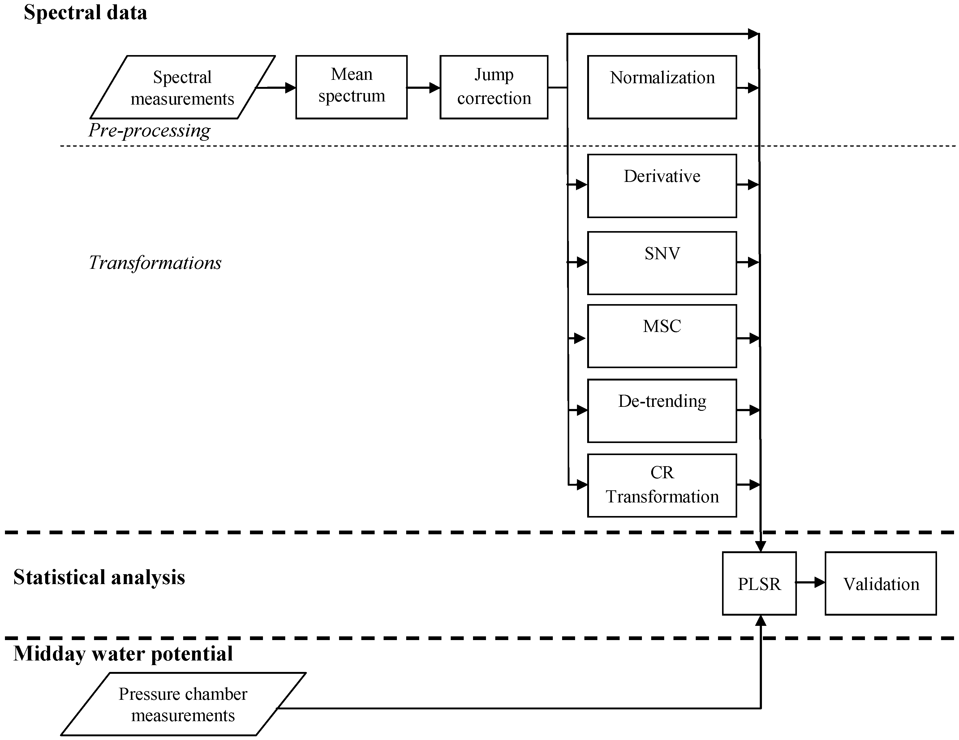
The methodology involved three main steps: Data acquisition (leaf water status and spectral measurements), data processing (pre-processing and spectral transformation), and statistical analyses (model fitting and validation) (Figure 2). Spectral data were collected immediately before leaf water status (water potential) measurement. The spectral data were pre-processed to obtain the mean spectral signatures of each leaf.
Six normalization methods were applied to reduce noise in the spectral data. Four derivative methods (GAP (Norris Gap) derivative and Savitzky–Golay derivative, both with first and second derivatives) and SNV, MSC, de-trending, and CR methods were used to study the relationship between the spectral data and LWP. PLSR was used to estimate leaf water status from the spectral data and the suitability of the regression models was assessed by cross-validation.

2.3. Leaf Water Status

Twelve vines per block were marked and 36 leaves were selected (mature leaves located opposite the first cluster of the central shoot). The selected leaves were picked immediately after measurement. For each leaf, midday LWP was measured using an SF-Pres-70 pressure chamber equipped with a digital manometer (Solfranc Tecnologías SL, Vilaseca, Tarragona, Spain).
Pressure chambers are widely used to measure water potential and pressure-volume ratios in leaves [40]. A pressure chamber applies pressure to a leaf to measure the flow rate of water for a given pressure drop between the inside and outside of the chamber [40]. The pressure necessary to extract sap from the leaf is an indicator of the leaf water status (a higher pressure means higher water stress).

2.4. Spectral Data

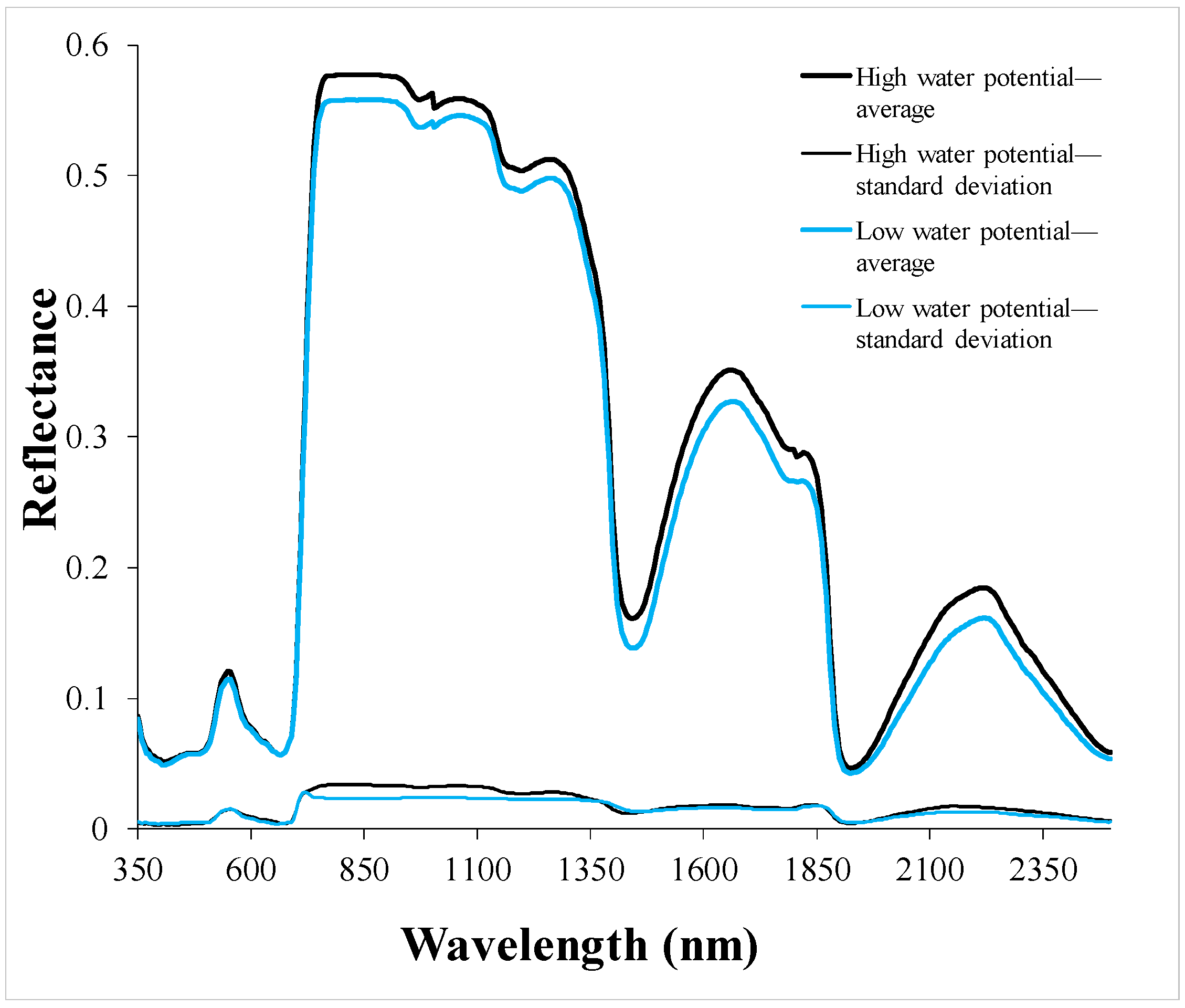
Spectral signatures were measured using an ASD FieldSpec 4 Portable Spectroradiometer (Analytical Spectral Devices, Inc., Boulder, CO, USA). This spectroradiometer captured spectral data at wavelength ranges of 350 nm and 2500 nm. Three detectors covered the required spectral range: A visible near-infrared (VNIR) silicon photodiode array (350–1000 nm) and two graded Indium Gallium Arsenide photodiode detectors for short-wavelength infrared (SWIR) measurement (1001–1800 nm and 1801–2500 nm). The arrangement of the radiometers caused jumps or splice points in the spectral signature that were not due to reflectance in the leaf; these jumps (at 1000 nm and at 1800 nm) are clearly visible in Figure 3. The ASD FieldSpec 4 used a flexible fibre optic cable to aim at the target.
In this work, the spectral measurements corresponded to reflectance, calculated as the ratio of the reflected energy of the observed leaf to the reflected energy of a known reference panel (sometimes called a calibration panel). This reference panel was a diffuse white reflectance panel that provided a diffuse homogeneous mix of all full source energy at nearly 100%.
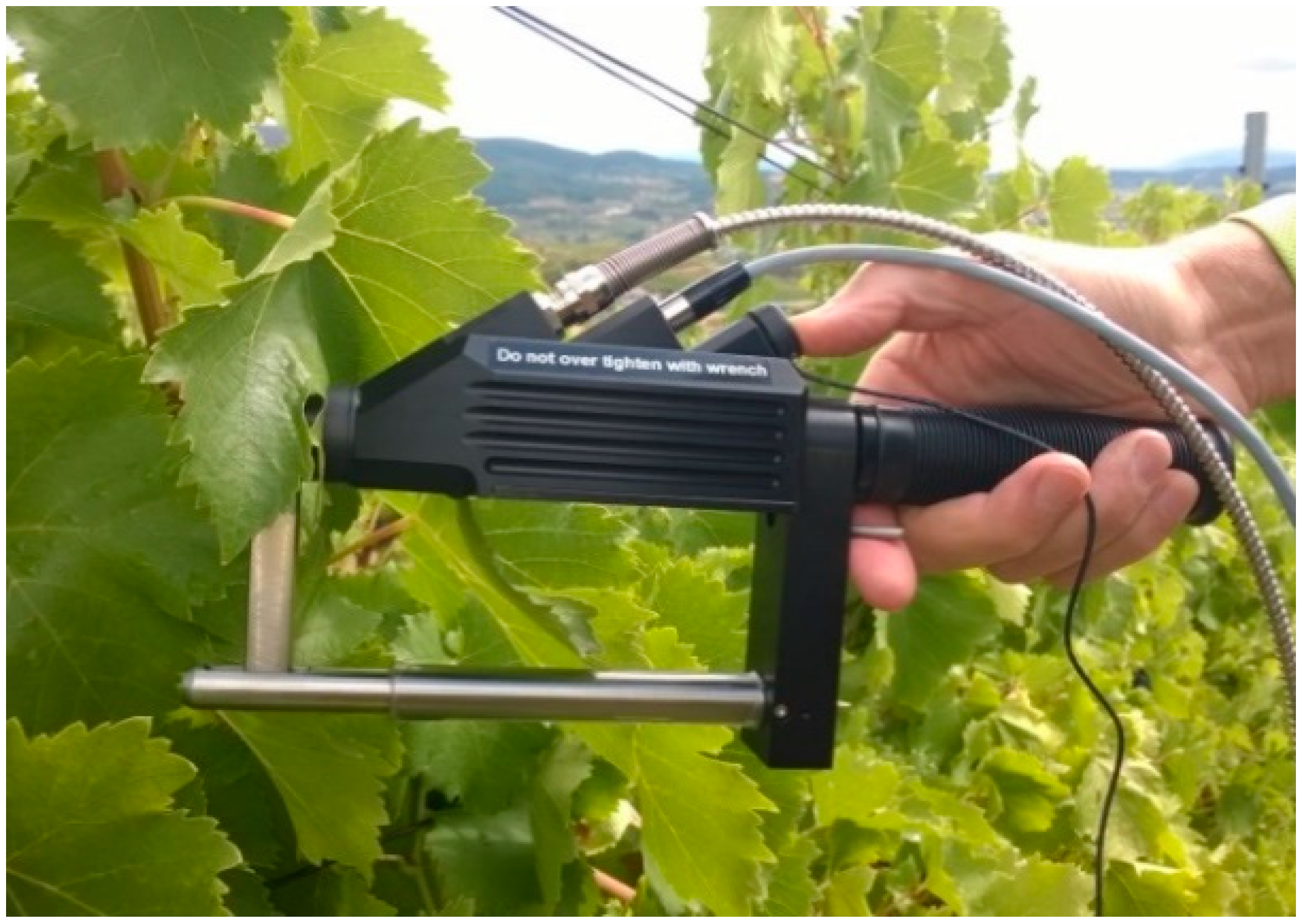
Data were collected following the recommendations of the spectroradiometer manufacturer [29]. Calibration was done with a white panel face and recalibration was done before measuring the first leaf of each block [29]. A plant probe was used to collect non-destructive spectral data from leaves. The plant probe accessory consisted of a low-intensity quartz-halogen bulb, a grip to position fibre-optic cable input to the spectroradiometer, and a quartz window to press the probe against the surface of interest [41]. The nominal spot size of the plant probe was 10 mm. A leaf clip was also used to hold the target leaf in position without removing it or inflicting damage, while allowing single-handed functionality (Figure 4).
Spectral data were collected from the upper face of the leaf. Measurements were done three times at three different points (avoiding veins, holes, and leaf spots) in order to ensure a representative spectrum of each leaf. Taking the spectral signature took about six seconds per each individual leaf.

2.4.1. Pre-Processing

Spectral reflectance data were checked using ViewSpect Pro6.0 software (Analytical Spectral Devices, Inc., Boulder, Colorado, USA) and exported to Spectral Analysis and Management System (SAMS) software 3.2 (Center for Spatial Technologies and Remote Sensing, University of California, Davis, CA, USA). Mean spectral signatures (one per leaf sample) were calculated. In order to mitigate the effects of mismatches between detectors, jump correction was applied at 1000 nm and 1800 nm, as follows: Bias values were calculated for the VNIR and SWIR2 regions and were used to offset the SWIR1 at the splice point. The resulting spectral data were normalized using Unscrambler®X 10.2 software and six different normalization techniques: (i) Area normalization, (ii) unit vector normalization, (iii) mean normalization, (iv) maximum normalization, (v) range normalization, and (vi) peak normalization.

2.4.2. Transformation

Spectral data pre-processed by a jump correction tool were transformed using five techniques: (i) Derivatives, (ii) SNV, (iii) MSC, (iv) de-trending, and (v) CR transformation. In this section, we describe an approach based on work described in the literature (mainly [32], but also [35,36]).
Baseline drift due to scattering (also referred to as the slope effect) and overlapping peaks were removed by applying derivative algorithms to the spectra. With this transformation, reflectance peaks were in the same place as in the original spectra [32]. Let the spectrum reflectance xi, be a function of wavelength λ. The derivative of the function is given as:
Zero order:
x i = f ( λ ) .
First order, taking the difference between the two wavelength bands:
d ( x i ) d λ = f ( λ ) = f ( λ i + 1 ) f ( λ i 1 ) 2 Δ λ .
Second order:
d 2 ( x i ) d λ 2 = f ( λ ) = f ( λ i + 2 ) 2 f ( λ i ) + f ( λ i 2 ) 4 Δ λ 2 ,
where Δλ is the difference between the λ values of adjacent data points.
Four derivative transformations were applied because the derivatives of the reflectance values allow differences between spectrum bands to be increased and also allow correction of the baseline effects [33]. The GAP derivative and Savitzky–Golay derivative were applied, using the first and second derivatives in both cases. The first derivative eliminated baseline displacements parallel to the abscissa axis, while the second derivative eliminated terms that varied linearly with the wavelength.
The SNV was used to locate multiplicative and additive interventions resulting from raw spectral data scatter and particle size variability. The scatter correction was a row-oriented transformation that standardized spectra using individual means and standard deviations. We first calculated the mean and standard deviation for each i spectrum of the m × 1 column vector xi. We then subtracted each data point in xij from the mean and divided it by the standard deviation [32]:
x i j   ( S N V ) = x i j x ¯ i s   ( x i ) .
MSC offers similar advantages to SNV in removing the baseline effect for both translation and offset in the spectra. Multiplicative and additive spectral corrections were applied to the original spectral data means, with the corrected spectra producing a relatively consistent baseline. For each j of m wavelengths, we calculated the mean of all n spectra, obtaining an m × 1 column vector of a standard spectrum m. We then performed simple linear regression xij = ai + bimj + eij on each i spectrum of the m × 1 column vector xi of n spectra in X (as the dependent variable), relative to the m × 1 vector m (as the independent variable). Given the solution obtained using the ordinary least square regression (OLSR) method, the regression coefficient parameter bi and intercept ai were used to correct baseline scatter by subtracting each spectrum xi from ai and dividing by bi [32]:
x i j   ( M S C ) = x i j a i b i .
De-trending accounts for variations in baseline shift and curvilinearity—generally found in the reflectance spectra of powdered or densely packed samples—using second-degree polynomial regression [30]. The procedure uses subtraction of the polynomial fit in each i spectrum. We define a second-order polynomial equation [32]:
x i j = a i + b i   λ j + c i   λ j 2 + e i j ,
where the intercept ai and the regression coefficient parameters bi and ci are determined using the OLSR method. The de-trended spectrum xij (detrend) is calculated as:
x j i ( d e t r e n d ) = x i j ( a i + b i   λ j + c i   λ j 2 ) ,
where λj is the band in j wavelength.
Derivative, SNV, MSC, and de-trending transformations were computed using Unscrambler®X 10.2 software. CR transformation identified and highlighted absorption features of interest [37], normalizing the reflectance spectra so that individual reflectance absorption features could be compared with a common baseline [38]. The CR transformations were computed using ENVI® 4.7 software (www.ittvis.com; IDL, Workbench).

2.5. Statistical Methods

Leaf water status estimation models were obtained by PLSR, which used continuous parts of the spectrum as input data.

2.5.1. Partial Least Squares Regression

To estimate leaf water status, PLSR was used to build models from the full spectrum. Multiple linear and stepwise regressions were applied along with several response variables simultaneously, correcting for collinearity and noisy independent variables [42]. PLSR functions by combining the most useful information from hundreds of bands into the first several factors, with the least important factors including background effects [37]. A smaller number of factors explaining most of the total variance in the data results in a simpler model architecture and greater prediction accuracy for the response variable [42]. Our criterion to add an additional factor to the model was that it had to reduce the root mean squared error (RMSE) by at least 2% to ensure model parsimony [24].
Measured water potential (MWP) was used as the predictor variable and pre-processed and transformed spectral data were used as the independent variable. Numerous correlations were analyzed, taking bands of different widths across the entire spectrum between 350 nm and 2500 nm. In terms of bandwidth, bands were taken from a very narrow bandwidth of 20 nm (twice the spectral resolution of the spectroradiometer) up to 2150 nm. In the middle, all bandwidths were incremented by an arbitrary step of 5 nm (twice the spectral resolution). The entire spectrum was run with all bandwidths in steps of 5 nm between bands. In total, 91,378 different PLRS correlations were analyzed for each dataset. The following datasets were considered:
(i)
MWP versus full reflectance spectrum from 350 nm to 2500 nm with jump correction.
(ii)
MWP versus full reflectance spectrum from 350 nm to 2500 nm with jump correction and area normalization.
(iii)
MWP versus full reflectance spectrum from 350 nm to 2500 nm with jump correction and unit vector normalization.
(iv)
MWP versus full reflectance spectrum from 350 nm to 2500 nm with jump correction and mean normalization.
(v)
MWP versus full reflectance spectrum from 350 nm to 2500 nm with jump correction and maximum normalization.
(vi)
MWP versus full reflectance spectrum from 350 nm to 2500 nm with jump correction and unit range normalization.
(vii)
MWP versus full reflectance spectrum from 350 nm to 2500 nm with jump correction and peak normalization.
(viii)
MWP versus full reflectance spectrum from 350 nm to 2500 nm with jump correction and Norris Gap first-order derivative.
(ix)
MWP versus full reflectance spectrum from 350 nm to 2500 nm with jump correction and Norris Gap second-order derivative.
(x)
MWP versus full reflectance spectrum from 350 nm to 2500 nm with jump correction and Savitzky–Golay first-order derivative.
(xi)
MWP versus full reflectance spectrum from 350 nm to 2500 nm with jump correction and Savitzky–Golay second-order derivative.
(xii)
MWP versus full reflectance spectrum from 350 nm to 2500 nm with jump correction and SNV.
(xiii)
MWP versus full reflectance spectrum from 350 nm to 2500 nm with jump correction and MSC.
(xiv)
MWP versus full reflectance spectrum from 350 nm to 2500 nm with jump correction and de-trending.
(xv)
MWP versus full reflectance spectrum from 350 nm to 2500 nm with jump correction and CR transformation.
PLSR estimates were made using the plsregress function in MATLAB software (MathWorks, Inc, Natick, MA, USA).

2.5.2. Cross-Validation

Model fit was validated comparing observed and expected values and using the k-fold cross-validation method. Cross-validation avoids overfitting by not reusing the same data to both fit a model and to estimate prediction error. In k-fold cross-validation, the original sample is systematically partitioned into k equal sized subsamples. Of the k subsamples, a single subsample is retained to test the model and the remaining k-1 subsamples are used to train the model. The cross-validation process is repeated k times, with each of the k subsamples used exactly once as the validation data. The k results can then be averaged to produce a single estimate. While 10-fold cross-validation is commonly used [43], in k-fold cross-validation, k is an unfixed parameter.
We analyzed the coefficient of determination (R2) and the RMSE in order to compare the fitted models [44]. Two consecutive PLSRs were executed. In the first PLSR, regressions with a maximum of 10 factors were calculated and k-fold cross-validation with k = 9 was computed. k = 9 was chosen instead of the traditional k = 10 because division of the 36 samples by 9 resulted in a whole number. Variation in the RMSE in cross-validation was analyzed using 1, 2, 3, etc. factors, in order to obtain the lowest RMSE value and, hence, the optimal number of factors to fit the water potential prediction models. In the second PLSR, the optimum number of factors as determined above was used, as was k-fold cross-validation, except, in this case, with k = 36 (equivalent to leave-one-out cross-validation); the models were thus constructed with 35 training samples, leaving one sample for the prediction. Prediction was repeated with each of the 36 samples and R2 was calculated by comparing the predicted and real water potential values.

3. Results

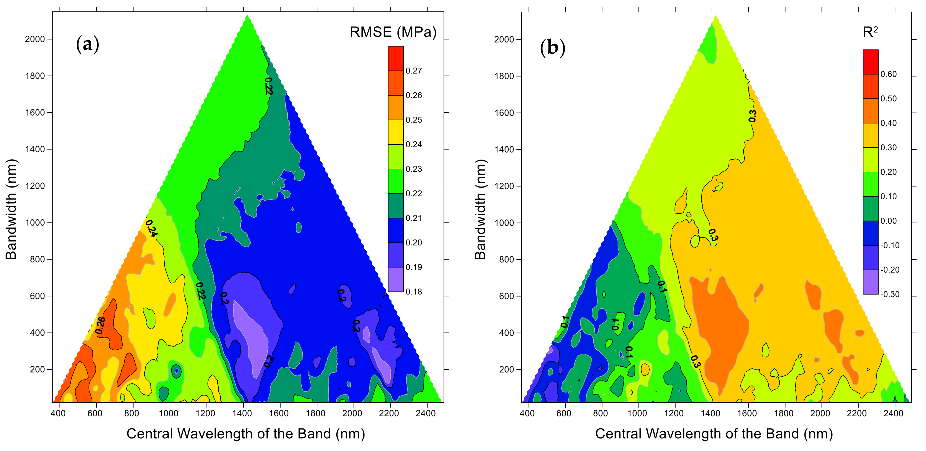
Figure 5 shows RMSE and R2 values for 91,378 PLSR water potential predictions compared with the corresponding reference data. RMSE is depicted in Figure 5a and R2 is depicted in Figure 5b. For the predictor variable (spectral data) no pre-processing was done other than jump correction. RMSE results were obtained directly from the plsregress Matlab function using cross-fold validation with k = 9. R2 values were obtained from another prediction round by combining the plsregress function and an in-house Matlab script with leave-one-out cross-validation. In Figure 5, the bandwidth considered in the PLSR is represented on the vertical axis, while the central wavelength of the band is shown on the horizontal axis. The top point in each triangle represents the result of a PLSR where the full spectrum (maximum width) was used and, logically, its central wavelength corresponds to the middle of the horizontal axis. All other points in the triangle represent RMSE and R2 values for different PLSR predictions of water potential and many spectral bands of varying widths and locations.
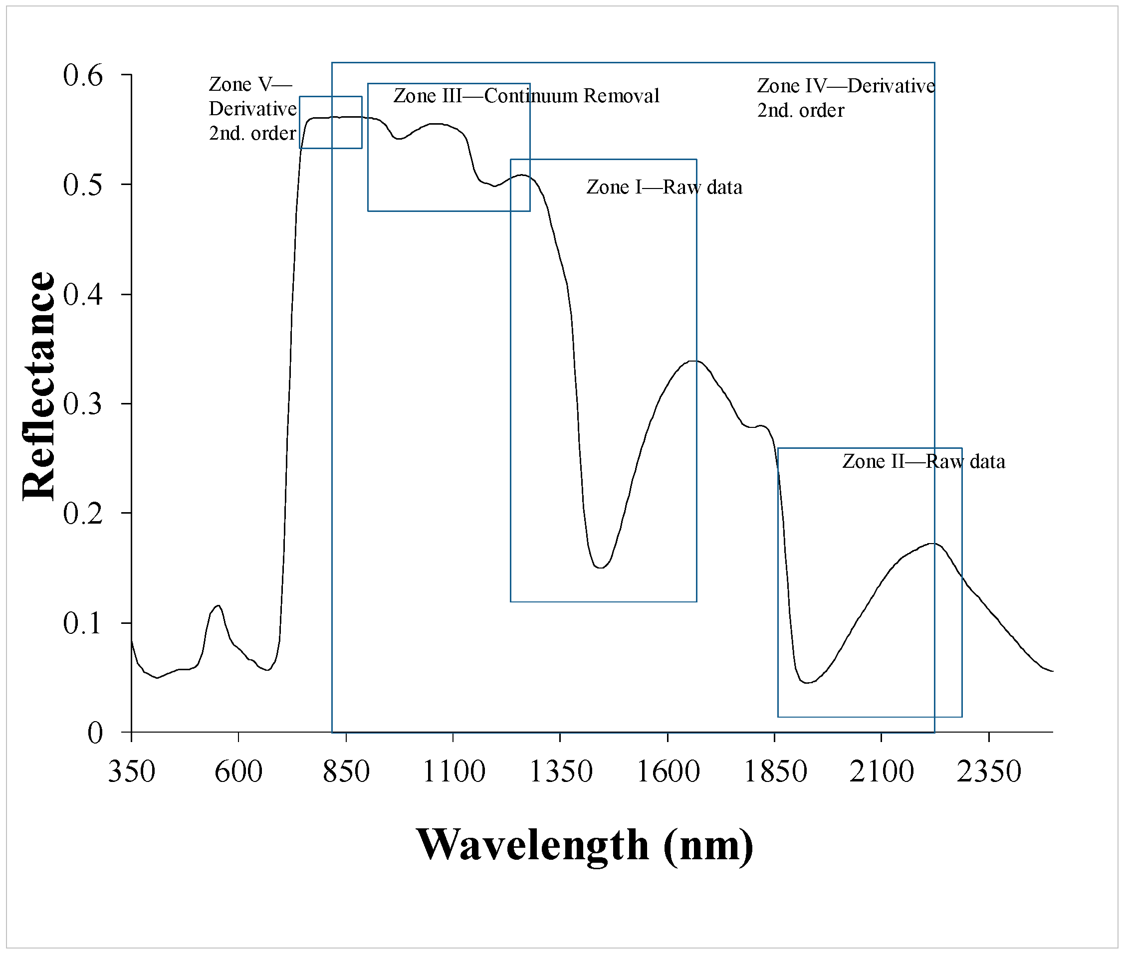
RMSE values were between 0.18 and 0.28 MPa. Considering that the reference data (36 samples) values ranged from −1.8 to −0.86 MPa, the best prediction areas had precisions of 10% to 22%. R2 ranged between negative values and 0.5. The negative R2 values areas were obtained with the lowest wavelengths, resulting in a model fit worse than a horizontal line. The highest R2 values did not exceed 0.5, which was a low value. However, certain areas showed better correlations than the rest, which clearly indicated that broad areas of the spectrum were undeniably correlated with water potential, specifically, at around 1450 nm for bandwidths of around 410 nm (Figure 6, Zone I) and, in the furthest part of the infrared, at 2060 nm for bandwidths of around 410 nm (Figure 6, Zone II).
The leaf water potential range was not as large as expected due to numerous rain events in the days before field data collection. August of 2017 was exceptionally rainy, with rainfall of 18.91 mm, over three times the average of the previous seven years (6.33 mm). Even so, the proposed method could work for a wide range of leaf water potential values.
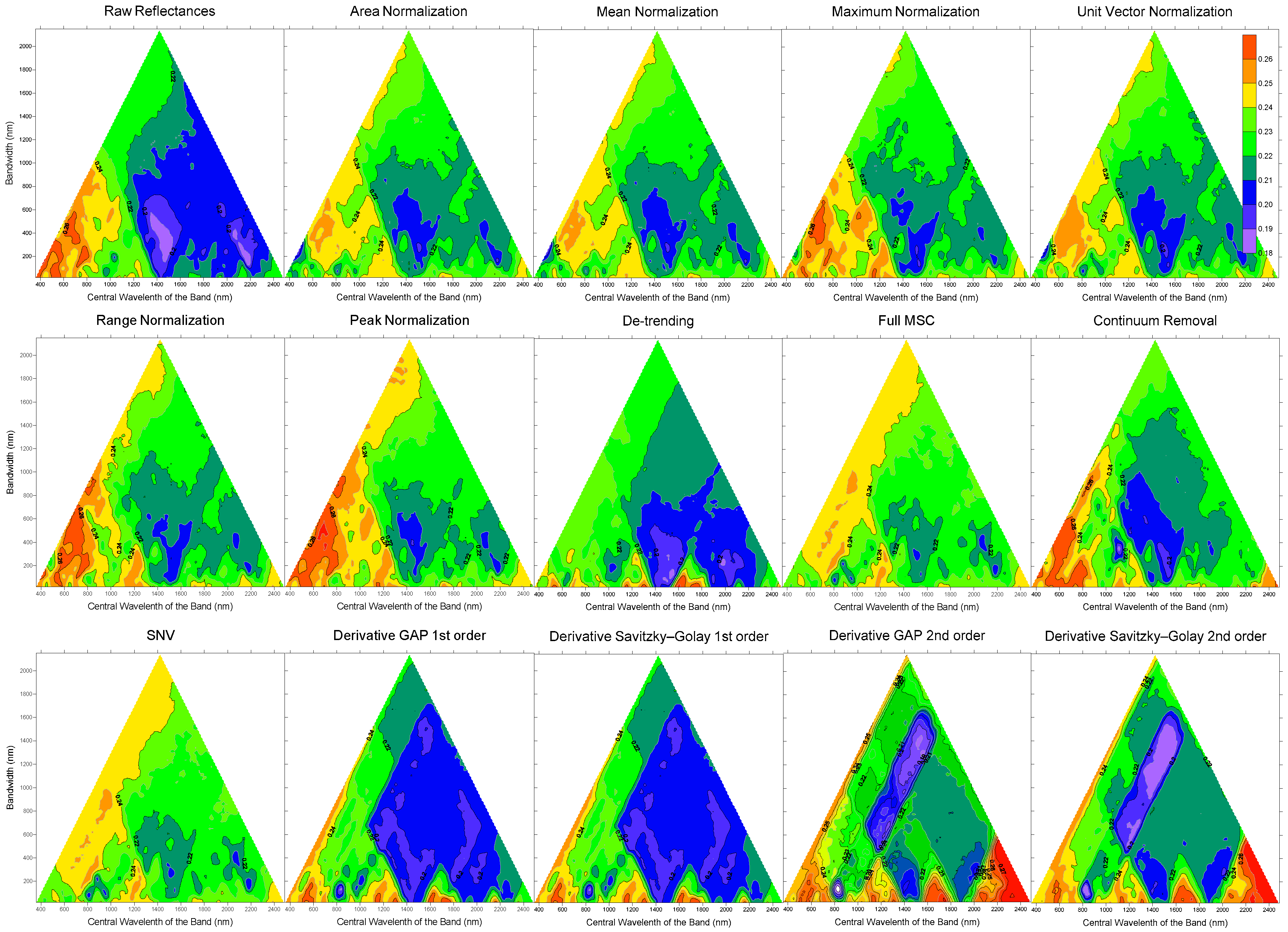
Part of this research consisted of studying the impact of different methods of pre-processing on correlations between measured water potential and spectral signatures. Figure 7 shows the RMSE obtained by the PLSR after applying the above-mentioned pre-processing treatments (normalization, de-trending, MSC, CR, SNV, and derivatives).
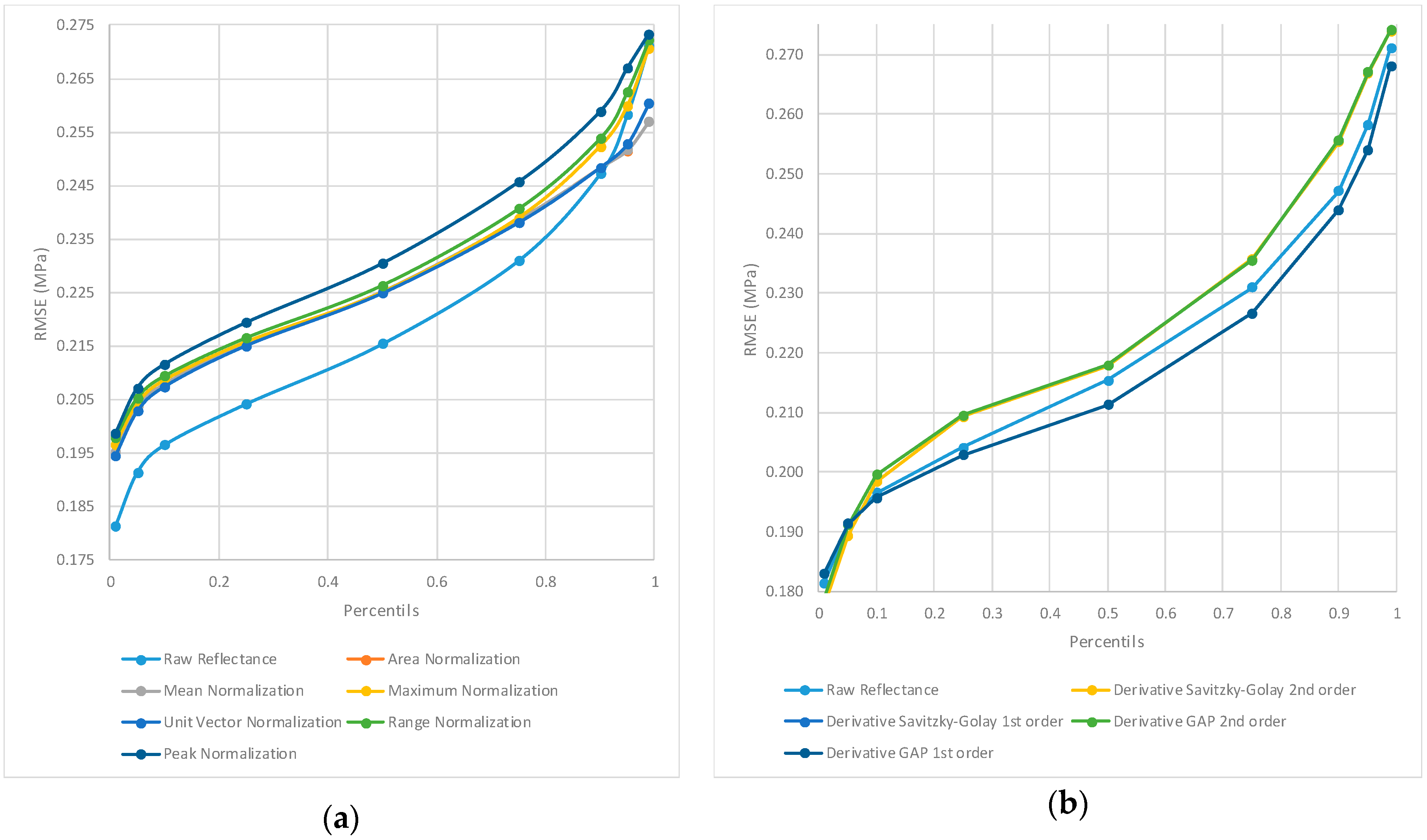
Applying normalization produced poor results because errors or residues (RMSE) tended to increase in the areas of maximum interest. As can be seen in Figure 8a, which shows errors obtained according to RMSE percentiles ordered from lowest to highest, minimum error increased with normalization pre-processing in 90% of cases. It was observed that the peak and mean pre-processing diminished maximum errors, although only in areas that were not of interest. De-trending, MSC, and SNV pre-processing did not seem to be very effective; in general, these pre-processing treatments reduced the areas of best and worst correlation results. CR pre-processing improved on the results of the other treatments but did not surpass the raw reflectance results. With CR pre-processing, a “hotspot” appeared with very low residues at around 1110 nm and with a relatively wide band of around 350 nm (Figure 6, Zone III).
Pre-processing with GAP and Savitzky–Golay derivatives returned very similar results for both first and second derivatives. Pre-processing with the first derivative reduced the RMSE in practically 99% of the correlations (Figure 8b). However, the second derivative reduced the lowest RMSEs, i.e., the most interesting cases, by only 1%. Pre-processing with the second derivative created a wide trapezoid-shaped area that contained optimal correlation results. The algid or optimum point of this zone consisted of a band centred on 1520 nm with a width of 1400 nm (Figure 6, Zone IV). Also resulting from second-derivative pre-processing was a narrow band (140 nm) located at 826 nm (Figure 6, Zone V). At this point, it was possible to find the best correlations. This zone also appeared for the first derivative, although slightly displaced to 835 nm and somewhat narrower (130 nm); however, it did not appear in the raw reflectance data without pre-processing, nor did it appear significantly in the rest of the pre-processed data.
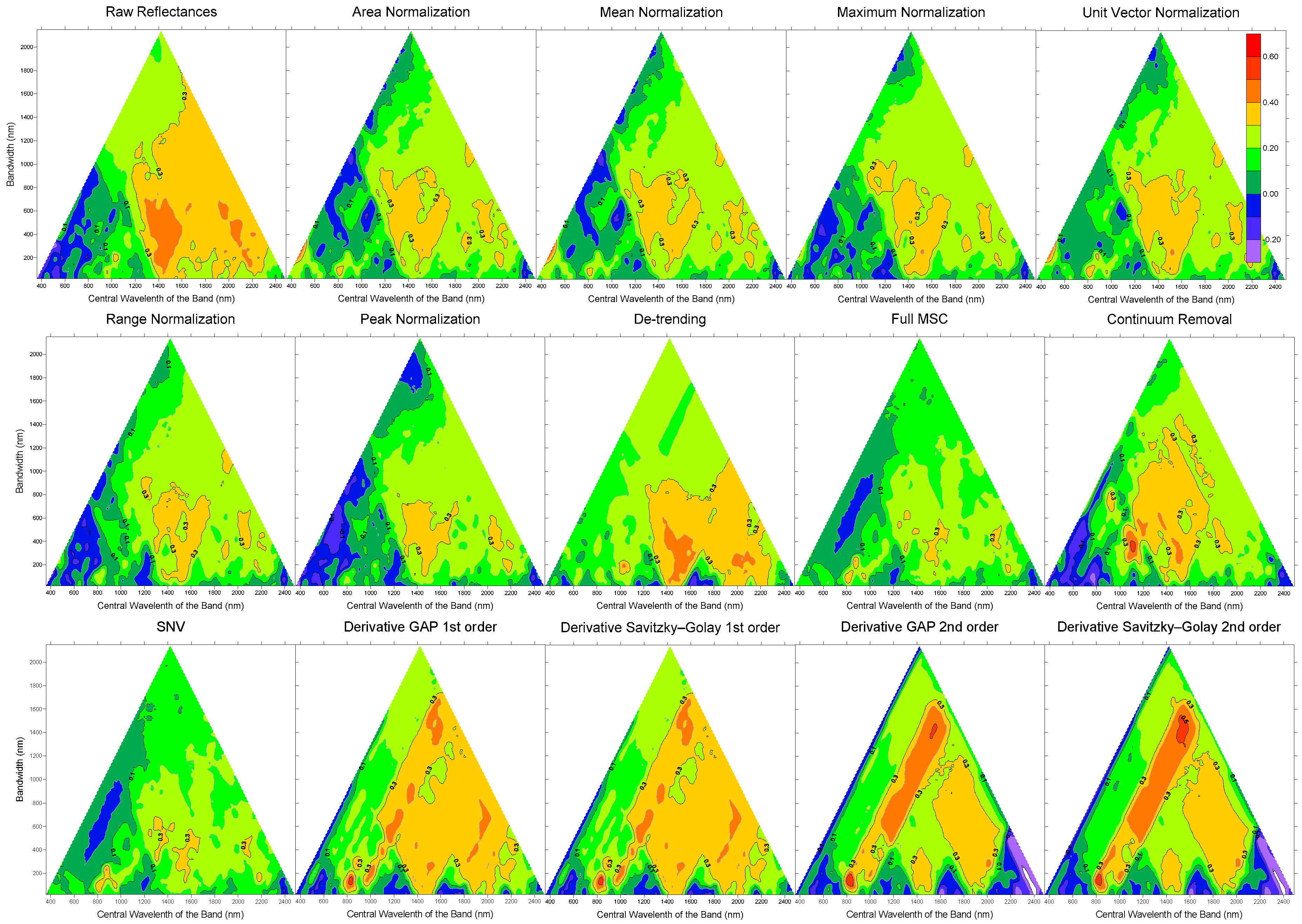
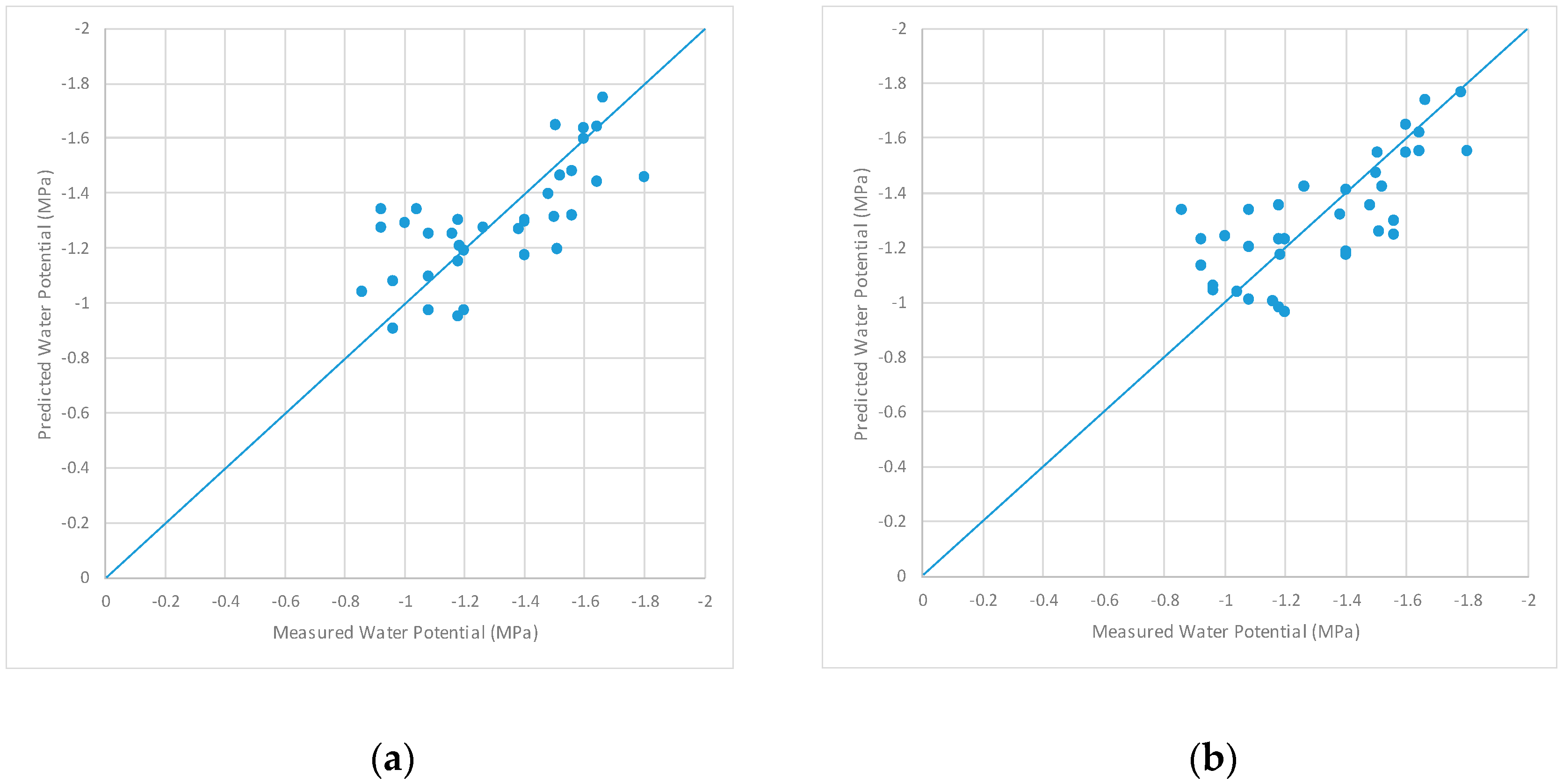
In general, the results for R2 (Figure 9) are equivalent to those for RMSE and, as expected, the zones with lower RMSE values coincided with higher R2 values. The R2 values obtained in the areas with the best correlations exceeded 0.50. Although not very high, it must be taken into account that prediction values were obtained through complete cross-validation, using the prediction for each and every one of the original samples to estimate R2. No sample of original field measurements was discarded as being an outlier or an abnormally high residual. Figure 10 shows an example of two specific PLRS water potential predictions in two of the more interesting spectral zones identified in this study; it was observed that the value of R2 using the data pre-processed using the Savitzky–Golay second-order derivative (R2 = 0.54) was slightly higher than the value using R2 and the raw data (R2 = 0.51). Moreover, RMSE values were lower for Savitzky–Golay second-order derivative models than for raw data models (0.18 and 0.20, respectively).

4. Discussion

After analzing a large number of PLSRs with bands of different widths throughout the available spectrum (350–2500 nm) and applying various pre-processing treatments, five spectral areas of interest were identified that allowed LWP for vines to be predicted with around 15%–20% accuracy. The results show that the areas of interest were obtained using near-infrared reflectance. These findings agree with several studies [8,25,45,46] that computed the most suitable relationship between spectral data and vine water content using wavelengths located in the near-infrared. The reason for this could be that wavelengths with maximum water absorption for crops are usually in the near-infrared [45]. The maximum water absorption point is shown in Figure 3, which depicts variations in the spectral signatures of leaves as a function of their water potential. The same figure shows that differences in reflectance between leaves with different water potentials were more evident in the near-infrared wavelengths than in the visible range.
The spectral areas of interest (Zones I and II in Figure 6), obtained from raw reflectance data without pre-processing, corresponded to the traditional absorption peaks, located at 1442 nm and 1928 nm, as frequently reported in previous works [8,46,47]. The numerous tests we carried out suggest that the optimum bandwidth to be used around these two absorption peaks spans from immediately before to immediately after the maximums. These zones have traditionally been used for the correlation of many variables related to water in plants [8,25,45,47].
Results generally deteriorated after normalization pre-processing. Errors or residues increased RMSE in the areas of maximum interest and in most of the bands. In some cases, normalization pre-processing reduced the maximum RMSE, but in bands that were not of interest. De-trending, MSC, and SNV pre-processing did not seem to be very effective either, as they increased the minimum RMSE but reduced the maximum RMSE. It seems that this kind of pre-processing tends to soften or average the spectra in some way, hiding some of the interesting differences in behaviours. Our results suggest that normalization pre-processing should not be used.
Pre-processing with GAP and Savitzky–Golay derivatives produced satisfactory results. While pre-processing with the first derivative reduced RMSE in practically 99% of the PLSR, pre-processing with the second derivative reduced the lowest RMSEs, i.e., the most interesting cases, by only 1%. Pre-processing with the second derivative resulted in a wide trapezoid-shaped area that contained optimal correlation results. The algid or optimum point of this zone consisted of a very wide band centred on 1520 nm and deriving from 820 nm to 2220 nm. This band, which we designated Spectral Zone IV, used practically all the near-infrared spectral data, which, as indicated above, reflected the greatest water absorption. The best correlations of all were found after second-derivative pre-processing in a narrow band (140 nm) located at 826 nm (Figure 6, Zone V). This zone also appeared after first-derivative pre-processing, although slightly displaced to 835 nm and somewhat narrower (130 nm). It did not appear in the raw reflectance data without pre-processing or to any significant degree in any other pre-processing. This corroborated results reported in the literature [8], where a relationship was found between leaf water content and spectral data in the area centred at 970 nm, suggesting this to be a typical area of crop water absorption; however, the weak relationship meant that this area was not the most suitable for determining LWP.
CR transformation improved on normalization, de-trending, MSC, and SNV results, but generally did not improve on raw reflectance results. With this pre-processing, a “hotspot” appeared with very low residues in 1110 nm, with a relatively wide band of around 350 nm (Figure 6, Zone III). This area of the spectrum contained two absorption peaks in a width of only 350 nm. However, as the hotspot was very small, bands with slightly different bandwidths or locations in the spectra showed the poorest results. This area therefore cannot be considered useful, despite very low residuals after applying CR, which may be why this area has not been reported before; nonetheless, more research needs to be done regarding this spectral zone. Note that CR pre-processing was designed for use in spectral intervals related to the absorption point of specific variables of plant composition (water, nitrogen, lignin, etc.) [25,45] and not in all spectral signatures; this may explain why CR transformation applied to the entire spectrum resulted in no improvement in the relationship between the spectral data and the variables.
While numerous works evaluated pre-processing of spectral data with a view of improving the prediction models of a variable [32,35,36], results varied depending on the type of variable that was determined and whether or not the pre-processing was combined with other kinds of pre-processing. Combination could explain the unsuitability of models computed with pre-processed spectral data. In our research, we used a single pre-processing treatment. Contrary to the other works, spectral pre-processing in our study did not improve R2, due to one of the most suitable prediction models being obtained with raw spectral data. Note that we collected spectral data using a plant probe accessory. Vegetation diversity and measurement conditions are two factors that have a great influence on spectral data collection [9]. When working in the field, it is normal to use passive sensors which require optimal lighting conditions, i.e., clear atmospheric conditions, with low aerosol content and water vapour in the atmosphere [48]; these sensors are also highly influenced by variations in solar or sensor zenith conditions, leaf movements due to wind, shadows in the crop, etc. Studies that predicted water content by spectrometry used smoothed and transformed spectral data to correct for measurement noise [5,26]. In our study, using a plant probe accessory minimized those effects because the plant probe had an integrated light source that allowed spectral data to be collected in full contact with the leaf and standardized lighting conditions [48], thereby allowing raw spectral data to be used to predict leaf water potential.
Looking at the most suitable models, the central wavelength was located at 1450 nm (using raw data) and at 826 nm and 1520 nm (using the second derivative). This result corroborated other works [5,26,47,49] which found that spectrum regions that included 1400 nm and1900 nm were best correlated with leaf composition variables. The reason could be because differences in reflectance values in the visible region (350–650 nm) of the leaf with differing water contents, while small, were greatest in the range 650–1400 nm, indicating this to have the most suitable intervals for detecting variations in water content [47]. These same bands corresponded to the first OH overtone excitation for H2O and the O–H and H–O–H deformation combination, whereas other bands corresponded to water content but also to cellulose and other organic components [50].
The most suitable model fitted with raw data (centred at 1450 nm) needed a bandwidth of 410 nm, while the two most suitable models fitted with derivative pre-processed data (centred at 826 nm and 1520 nm) needed bandwidths of 140 nm and 1400 nm, respectively. These results concurred with the findings of research that applied CR transformation in several ranges of the spectrum to estimate leaf water content in four vine varieties [8]. Those authors computed CR in four water absorption ranges centred on 960 nm (with range 205 nm), 1190 nm (with range 151 nm), 1465 nm (with range 403 nm), and 2035 nm (with range 410 nm) and used CR-transformed spectral data and PLSR to obtain suitable vine water prediction models. Thus, the central wavelength and bandwidths were similar in both those studies and our own. In addition, Figure 7 and Figure 9 show the maximum R2 and minimum RMSE for the model computed using CR pre-processing, with the centred wavelength and bandwidth coinciding with the CR interval selected for the above-mentioned work and for the most suitable model obtained in our study. This corroborates what was stated above; CR pre-processing was specifically designed to apply to spectral intervals related to the absorption point for variables, including water, nitrogen, lignin, etc. Figure 10 shows that, although the differences are small, models computed using Savitzky–Golay second-order derivative were slightly more appropriate than models fitted using raw data.
Our results indicate the importance of proper selection of wavelength, bandwidth, and pre-processing methods in developing a prediction model. Future research could examine combinations of normalization and other pre-processing methods with a view of improving the relationships between spectral data and vine water potential and developing an accurate, rapid, and non-destructive approach to detecting water stress in vineyards.

5. Conclusions

Our research, in which we tested different pre-processing methods for spectral data and identified the wavelength range that minimized RMSE values, demonstrates the usefulness of field spectroscopy for estimating midday water potential in vines.
The results show that derivative pre-processing increases the determination coefficients and reduces RMSE. A model fitted with raw data obtains the best results for the range centred on 1450 nm (bandwidth 410 nm), while a model fitted with derivative pre-processed data obtains the best results for bands centred on 826 nm (bandwidth 140 nm) and 1520 nm (bandwidth 1400 nm).
The proposed method has some advantages with respect to other methods, mainly that the field work is simple, rapid, and non-destructive. However, it has some drawbacks, such as the need to pre-process the reflectance data and the model fit.
In short, field spectroscopy is a means to evaluate water stress level in vines, which could be useful in optimizing irrigation scheduling and managing remote sensing systems.

Author Contributions

Conceptualization: J.R.R.-P. and V.M.G.; methodology: J.R.R.-P., A.B.G.-F. and M.G.-F.; software: E.S.-A.; formal analysis: E.S.-A. and A.B.G.-F.; writing—original draft preparation: A.B.G.-F., M.G.-F., E.S.-A. and J.R.R.-P.; writing—review and editing: A.B.G.-F., J.R.R.-P. and E.S.-A.; visualization: E.S.-A. and V.M.G.; supervision and project administration: J.R.R.-P.

Funding

This research was funded by the Education Department of the Junta de Castilla y León, grant number LE112G189.

Acknowledgments

This research was supported by funding from the Education Department of the Junta de Castilla y León (grant number LE112G189, Order 20 November 2017), under a call for research by recognized research groups attached to public universities starting in 2018). The authors acknowledge the assistance of Miguel Marabel and Joana Rubio (Matarromera Group SL) in the field work.

Conflicts of Interest

The authors declare no conflict of interest. The funders had no role in the design of the study; in the collection, analyses, or interpretation of data; in the writing of the manuscript, or in the decision to publish the results.

References

  1. Flexas, J.; Galmés, J.; Gallé, A.; Gulias, J.; Pou, A.; Ribas, M.; Tomàs, M.; Medrano, H. Improving water use efficiency in grapevines: Potential physiological targets for biotechnological improvement. Aust. J. Grape Wine Res. 2010, 16, 106–121. [Google Scholar] [CrossRef]
  2. Lisar, S.Y.S.; Motafakkerazad, R.; Hossain, M.M.; Rahman, I.M.M. Water stress in plants: Causes, effects and responses. In Water Stress; Ismail, M.M.R., Hiroshi, H., Eds.; Intech Open: Rijeka, Croatia, 2012; pp. 1–15. [Google Scholar]
  3. Kennedy, J.A.; Matthews, M.A.; Waterhouse, A.L. Effect of maturity and vine water status on grape skin and wine flavonoids. Am. Enol. Vitic. 2002, 53, 268–274. [Google Scholar]
  4. Scholander, P.F.; Hammel, H.J.; Bradstreet, A.; Hemmingsen, E.A. Sap pressure in vascular plants. Science 1965, 148, 339–346. [Google Scholar] [CrossRef] [PubMed]
  5. Santos, A.O.; Kaye, O. Grapevine leaf water potential based upon near infrared spectroscopy. Sci. Agric. 2009, 66, 287–292. [Google Scholar] [CrossRef] [Green Version]
  6. Triolo, R.; Roby, J.P.; Plaia, A.; Hilbert, G.; Buscemi, S.; Di Lorenzo, R.; van Leeuwen, C. Hierarchy of factors impacting grape berry mass: Separation of direct and indirect effects on major berry metabolites. Am. J. Enol. Vitic. 2018, 69, 103–112. [Google Scholar] [CrossRef]
  7. Oumar, Z.; Mutanga, O. Predicting plant water content in Eucalyptus grandis forest stands in KwaZulu-Natal, South Africa using field spectra resampled to the Sumbandila Satellite Sensor. Int. J. Appl. Earth Obs. Geoinf. 2010, 12, 158–164. [Google Scholar] [CrossRef]
  8. Serrano, L.; Gonzalez-Flor, C.; Gorchs, G. Assessing vineyard water status using the reflectance-based water index. Agric. Ecosyst. Environ. 2010, 139, 490–499. [Google Scholar] [CrossRef]
  9. Zheng, L.; Wang, Z.; Sun, H.; Zhang, M.; Li, M. Real-time evaluation of corn leaf water content based on the electrical property of leaf. Comput. Electron. Agric. 2015, 112, 102–109. [Google Scholar] [CrossRef]
  10. Fuentes, A.; Vázquez-Gutiérrez, J.L.; Pérez-Gago, M.B.; Vonasek, E.; Nitin, N.; Dian, M.B. Application of non-destructive impedance spectroscopy to determination of the effect of temperature on potato microstructure and texture. J. Food Eng. 2014, 133, 16–22. [Google Scholar] [CrossRef]
  11. Jamaludin, D.; Abd-Aziz, S.; Ahmad, D.; Jaafar, H.Z.E. Impedance analysis of Labisia pumila plant water status. Inf. Process. Agric. 2015, 2, 161–168. [Google Scholar] [CrossRef]
  12. Mizukami, Y.; Sawai, Y.; Yamaguchi, Y. Moisture Content Measurement of Tea Leaves by Electrical Impedance and Capacitance. Biosyst. Eng. 2006, 93, 293–299. [Google Scholar] [CrossRef]
  13. He, J.-X.; Wang, Z.-Y.; Shi, Y.-L.; Qin, Y.; Zhao, D.-J.; Huang, L. A Prototype Portable System for Bioelectrical Impedance Spectroscopy. Sens. Lett. 2011, 9, 1151–1156. [Google Scholar] [CrossRef]
  14. Muñoz-Huerta, R.F.; Ortiz-Melendez, A.; Guevara-Gonzalez, R.G.; Torres-Pacheco, I.; Herrera-Ruiz, G.; Contreras-Medina, L.M.; Prado-Olivarez, J.V.; Ocampo-Velázquez, R. An Analysis of Electrical Impedance Measurements Applied for Plant N Status Estimation in Lettuce (Lactuca sativa). Sensors 2014, 14, 11492–11503. [Google Scholar] [CrossRef]
  15. Zimmermann, U.; Rüger, S.; Shapira, O.; Westhoff, M.; Wegner, L.-H.; Reuss, R.; Geßner, P.; Zimmermann, G.; Israeli, Y.; Zhou, A.; et al. Effects of environmental parameters and irrigation on the turgor pressure of banana plants measured using the non-invasive, online monitoring leaf patch clamp pressure probe. Plant Biol. 2010, 12, 424–436. [Google Scholar] [CrossRef]
  16. Rueger, S.; Ehrenberger, W.; Zimmermann, U.; Ben-Gal, A.; Agam, N.; Kool, D. The leaf patch clamp pressure probe: A new tool for irrigation scheduling and deeper insight into olive drought stress physiology. Acta Hortic. 2011, 888, 223–230. [Google Scholar] [CrossRef]
  17. Sancho-Knapik, D.; Gismero, J.; Asensio, A.; Peguero-Pina, J.J.; Fernández, V.; Gómez Álvarez-Arenas, T.; Gil-Pelegrín, E. Microwave l-band (1730 MHz) accurately estimates the relative water content in poplar leaves. A comparison with a near infrared water index (R1300/R1450). Agric. For. Meteorol. 2011, 151, 827–832. [Google Scholar] [CrossRef]
  18. Sancho-Knapik, D.; Gómez Álvarez-Arenas, T.; Peguero-Pina, J.J.; Gil-Pelegrín, E. Air-coupled broadband ultrasonic spectroscopy as a new non-invasive and non-contact method for the determination of leaf water status. J. Exp. Bot. 2010, 61, 1385–1391. [Google Scholar] [CrossRef] [Green Version]
  19. Sancho-Knapik, D.; Peguero-Pina, J.J.; Medrano, H.; Fariñas, M.D.; Gómez Álvarez-Arenas, T.; Gil-Pelegrín, E. The reflectivity in the S-band and the broadband ultrasonic spectroscopy as new tools for the study of water relations in Vitis vinifera L. Physiol. Plant. 2013, 148, 512–521. [Google Scholar] [CrossRef]
  20. Moshou, D.; Pantazi, X.; Kateris, D.; Gravalos, I. Water stress detection based on optical multisensor fusion with a least squares support vector machine classifier. Biosyst. Eng. 2014, 117, 15–22. [Google Scholar] [CrossRef]
  21. Hall, A.; Lamb, D.W.; Holzapfel, B.P.; Louis, J.P. Within-season temporal variation in correlations between vineyard canopy and wine grape composition and yield. Precis. Agric. 2011, 12, 103–117. [Google Scholar] [CrossRef]
  22. Strever, A.E. Estimating water stress in Vitis vinifera L. using field spectrometry: A preliminary study incorporating multispectral vigour classification. In Information and technology for sustainable fruit and vegetable production. In Proceedings of the Conference FRUTIC, Montpellier, France, 12–16 September 2005. [Google Scholar]
  23. Atzberger, C.; Guérif, M.; Baret, F.; Werner, W. Comparative analysis of three chemometric techniques for the spectroradiometric assessment of canopy chlorophyll content in winter wheat. Comput. Electron. Agric. 2010, 73, 165–173. [Google Scholar] [CrossRef]
  24. Cho, M.A.; Skidmore, A.; Corsi, F.; Van Wieren, S.E.; Sobhan, I. Estimation of green grass/herb biomass from airborne hyperspectral imagery using spectral indices and partial least squares regression. Int. J. Appl. Earth Obs. Geoinf. 2007, 9, 414–424. [Google Scholar] [CrossRef]
  25. González-Fernández, A.B.; Rodríguez-Pérez, J.R.; Marabel, M.; Álvarez-Taboada, F. Spectroscopic estimation of leaf water content in commercial vineyards using continuum removal and partial least squares regression. Sci. Hortic. 2015, 188, 15–22. [Google Scholar] [CrossRef]
  26. Zhang, Q.; Li, Q.; Zhang, G. Rapid determination of leaf water content using VIS/NIR spectroscopy analysis with wavelength selection. J. Spectrosc. 2012, 27, 93–105. [Google Scholar] [CrossRef]
  27. Mirzaie, M.; Darvishzadeh, R.; Shakiba, A.; Matkan, A.A.; Atzberger, C.; Skidmore, A. Comparative analysis of different uni- and multi-variate methods for estimation of vegetation water content using hyper-spectral measurements. Int. J. Appl. Earth Obs. Geoinf. 2014, 26, 1–11. [Google Scholar] [CrossRef]
  28. Zhao, K.; Valle, D.; Popescu, S.; Zhang, X.; Mallick, B. Hyperspectral remote sensing of plant biochemistry using Bayesian model averaging with variable and band selection. Remote Sens. Environ. 2013, 132, 102–119. [Google Scholar] [CrossRef]
  29. ASD Inc. 2012 FieldSpect4 User Manual 600979. Available online: https://www.malvernpanalytical.com/en/learn/knowledge-center/user-manuals/fieldspec-4-user-guide (accessed on 9 May 2019).
  30. Barnes, R.J.; Dhanoa, M.S.; Susan, S.J. Standard normal variate transformation and de-trending of near-infrared diffuse reflectance spectra. Appl. Spectrosc. 1989, 43, 772–777. [Google Scholar] [CrossRef]
  31. Vasques, G.M.; Grunwald, S.; Sickman, J.O. Comparison of multivariate methods for inferential modeling of soil carbon using visible/near-infrared spectra. Geoderma 2008, 146, 14–25. [Google Scholar] [CrossRef]
  32. Silalahia, D.D.; Midib, H.; Arasanb, J.; Mustafab, M.S.; Calimana, J.P. Robust generalized multiplicative scatter correction algorithm on pre-processing of near infrared spectral data. Vib. Spectrosc. 2018, 97, 55–65. [Google Scholar] [CrossRef]
  33. Norris, K.H.; Williams, P.C. Optimization of mathematical treatments of raw near-infrared signal in the measurement of protein in hard red spring wheat. i. influence of particle size. Cereal Chem. 1984, 61, 158–165. [Google Scholar]
  34. CAMO Software AS. The Unscrambler® X v10.3. User Manual. Version 1.0. Available online: https://www.camo.com/files/TheUnscramblerXv10.3-UserManual.zip (accessed on 9 May 2019).
  35. Syvilay, D.; Wilkie-Chancellier, N.; Trichereau, B.; Texier, A.; Martínez, L.; Serfaty, S.; Detalle, V. Evaluation of the standard normal variate method for Laser-Induced Breakdown Spectroscopy data treatment applied to the discrimination of painting layers. Spectrochim. Acta B 2015, 114, 38–45. [Google Scholar] [CrossRef]
  36. Maleki, M.R.; Mouazen, A.M.; Ramon, H.; De Baerdemaeker, J. Multiplicative scatter correction during on-line measurement with near infrared spectroscopy. Biosyst. Eng. 2007, 96, 427–433. [Google Scholar] [CrossRef]
  37. Huang, Z.; Turner, B.J.; Dury, S.J.; Wallis, I.R.; Foley, W.J. Estimating foliar nitrogen concentration from HYMAP data using continuum removal analysis. Remote Sens. Environ. 2004, 93, 18–29. [Google Scholar] [CrossRef]
  38. Kokaly, R.F.; Asner, G.P.; Ollinger, S.V.; Martin, M.E.; Wessman, C.A. Characterizing canopy biochemistry from imaging spectroscopy and its application to ecosystem studies. Remote Sens. Environ. 2009, 113, S78–S91. [Google Scholar] [CrossRef]
  39. Rodríguez-Pérez, J.R.; Riaño, D.; Carlisle, E.; Ustin, S.; Smart, D.R. Evaluation of hyperspectral reflectance indexes to detect grapevine water status in vineyards. Am. J. Enol. Vitic. 2007, 58, 302–317. [Google Scholar]
  40. Turner, N.C. Measurement of plant water status by the pressure chamber technique. Irrig. Sci. 1988, 9, 289–308. [Google Scholar] [CrossRef]
  41. Lau, I.C.; Cudahy, T.J.; Heinson, G.; Mauger, A.J.; James, P.R. Practical applications of hyperspectral remote sensing in regolith research. In Advances in Regolith; Roach, I.C., Ed.; CRC LEME: Adelaide, Australia, 2003; pp. 249–253. [Google Scholar]
  42. Geladi, P.; Kowalski, B.R. Partial least-squares regression: A tutorial. Anal. Chim. Acta 1986, 185, 1–17. [Google Scholar] [CrossRef]
  43. McLachlan, G.J.; Do, K.A.; Ambroise, C. Analyzing Microarray Gene Expression Data, 1st ed.; Wiley: New York, NY, USA, 2004; pp. 61–97. [Google Scholar]
  44. Richter, K.; Atzberger, C.; Hank, T.B.; Mauser, W. Derivation of biophysical variables from Earth observation data: Validation and statistical measures. J. Appl. Remote Sens. 2012, 6, 1–23. [Google Scholar] [CrossRef]
  45. Kokaly, R.F.; Clark, R.N. Spectroscopic determination of leaf biochemistry using band-depth analysis of absorption features and stepwise multiple linear regression. Remote Sens. Environ. 1999, 67, 267–287. [Google Scholar] [CrossRef]
  46. González-Fernández, A.B.; Rodríguez-Pérez, J.R.; Marcelo, V.; Valenciano, J.B. Using field spectrometry and a plant probe accessory to determine leaf water content in commercial vineyards. Agric. Water Manag. 2015, 156, 43–50. [Google Scholar] [CrossRef]
  47. Rodríguez-Pérez, J.R.; Ordóñez, C.; González-Fernández, A.B.; Sanz-Ablanedo, E.; Valenciano, J.B.; Marcelo, V. Leaf water content estimation by functional linear regression of field spectroscopy data. Biosyst. Eng. 2018, 36–46. [Google Scholar] [CrossRef]
  48. Milton, E.J.; Schaepman, M.E.; Anderson, K.; Kneubühler, M.; Fox, N. Progressing field spectroscopy. Remote Sens. Environ. 2009, 113, S92–S109. [Google Scholar] [CrossRef]
  49. Wang, J.; Xu, R.; Yang, S. Estimation of plant water content by spectral absorption features centered at 1450 nm and 1940 nm regions. Environ. Monit. Assess. 2009, 157, 459–469. [Google Scholar] [CrossRef]
  50. Shenk, J.S.; Workman, J.; Westerhaus, M.O. Application of NIR spectroscopy to agricultural products. In Handbook of Near-Infrared Analysis (Practical Spectroscopy Series), 2nd ed.; Burns, D.A., Ciurczak, E.D., Eds.; Dekker: New York, NY, USA, 2001; pp. 419–474. [Google Scholar]
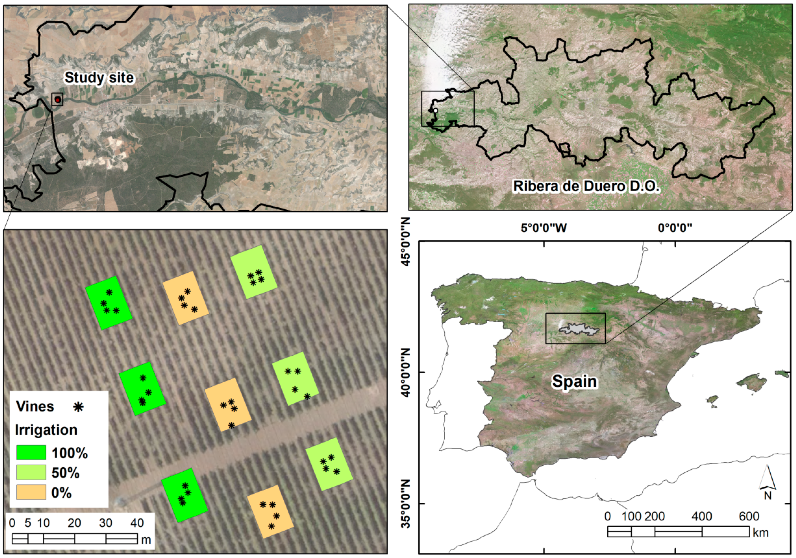
Figure 1. Study vineyard showing blocks and vine locations. D.O.: Ribera de Duero Designation of Origin.
Agronomy 09 00427 g001
Figure 2. Flowchart depicting midday water potential estimation by spectroscopy. SNV: standard normal variate; MSC: multiplicative scatter correction; CR: Continuum Removal; PLSR: Partial Least Square Regression.
Agronomy 09 00427 g002
Figure 3. Spectral signatures of leaves with high water potential (black line) and low water content (blue line). The spectral signatures were drawn from seven samples each for the highest and the lowest water potential.
Agronomy 09 00427 g003
Figure 4. Spectral data collection using a plant probe and leaf clip accessories.
Agronomy 09 00427 g004
Figure 5. (a) Root mean square error (RMSE) and (b) R2 of 91,378 partial least squares regression (PLSR) predictions of water potential for all 36 samples using raw spectral reflectance data.
Agronomy 09 00427 g005
Figure 6. Relevant zones obtained in this study.
Agronomy 09 00427 g006
Figure 7. RMSE values for water potential (MPa) obtained by PLSR using raw reflectance data and after pre-processing (area, mean, maximum, unit vector, range, and peak variants of normalization, de-trending, MSC, CR, SNV, and GAP and Savitzky–Golay first- and second-order derivatives). All graphs apply the same colour scale (see legend in the top-right corner).
Agronomy 09 00427 g007
Figure 8. Maximum errors ordered by RMSE percentile from lowest to highest. The lower curves show a higher number of correlations with lower residuals. (a) Raw reflectance versus normalization pre-processing. (b) Raw reflectance versus derivative pre-processing.
Agronomy 09 00427 g008
Figure 9. R2 values obtained by PLSR using raw reflectance data and after pre-processing (area, mean, maximum, unit vector, range, and peak variants of normalization, de-trending, MSC, CR, SNV, and GAP and Savitzky-Golay first- and second-order derivatives). All graphs apply the same colour scale (see legend in the top-right corner).
Agronomy 09 00427 g009
Figure 10. PLSR water potential prediction versus reference data in (a) a band 410 nm wide centred on 1265 nm (Zone I) for raw spectral data and (b) a band 1432 nm wide centred on 1552 nm (Zone IV) after applying Savitzky–Golay second-order derivative pre-processing. Data in (a) were fit to R2 = 0.51 and an RMSE of 0.20, while data in (b) were fit to R2 = 0.54 and an RMSE of 0.18.
Agronomy 09 00427 g010