Estimating Body Condition Score in Dairy Cows From Depth Images Using Convolutional Neural Networks, Transfer Learning and Model Ensembling Techniques

 , , , and
Abstract
1. Introduction
2. Materials and Methods
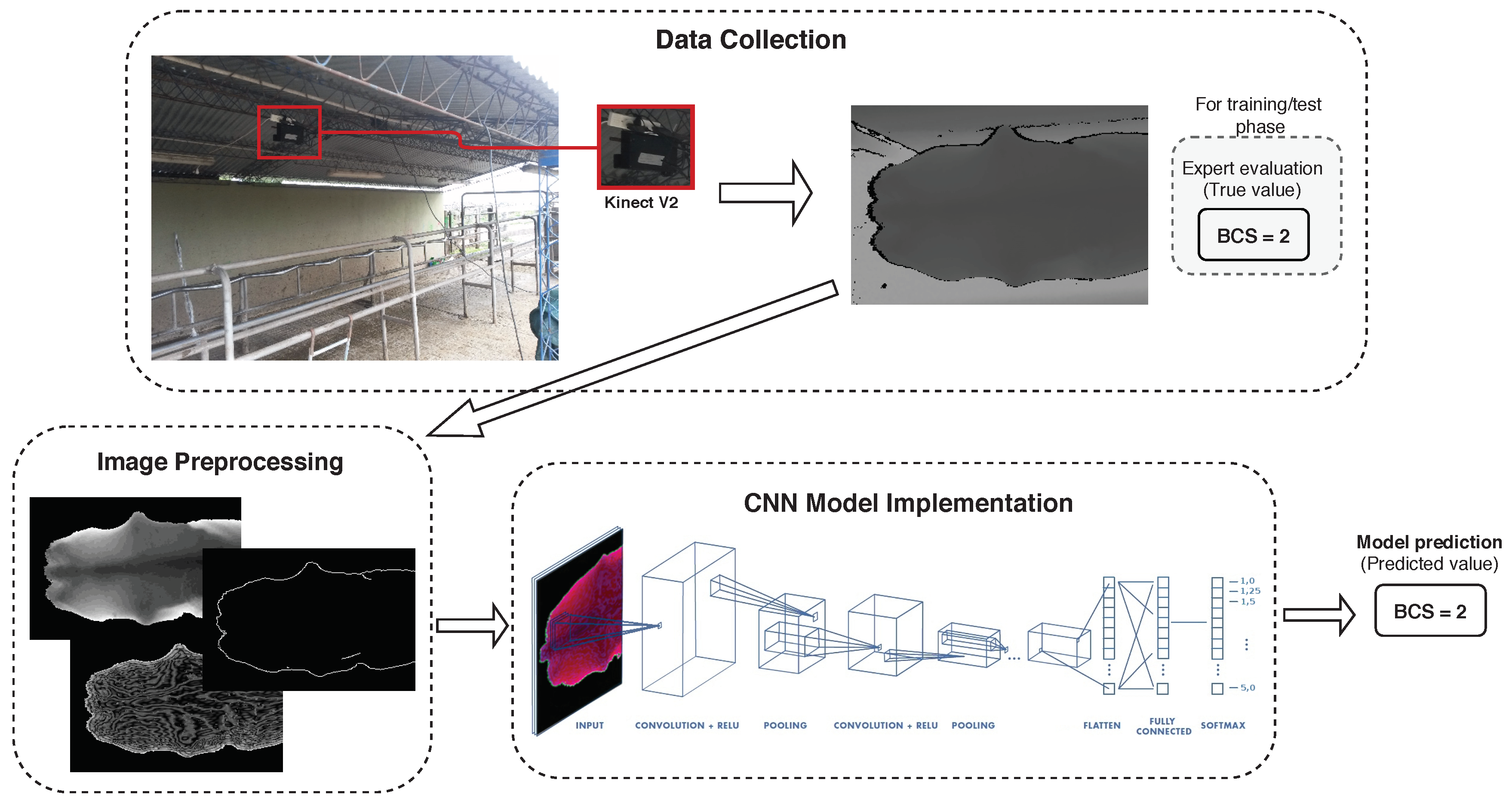
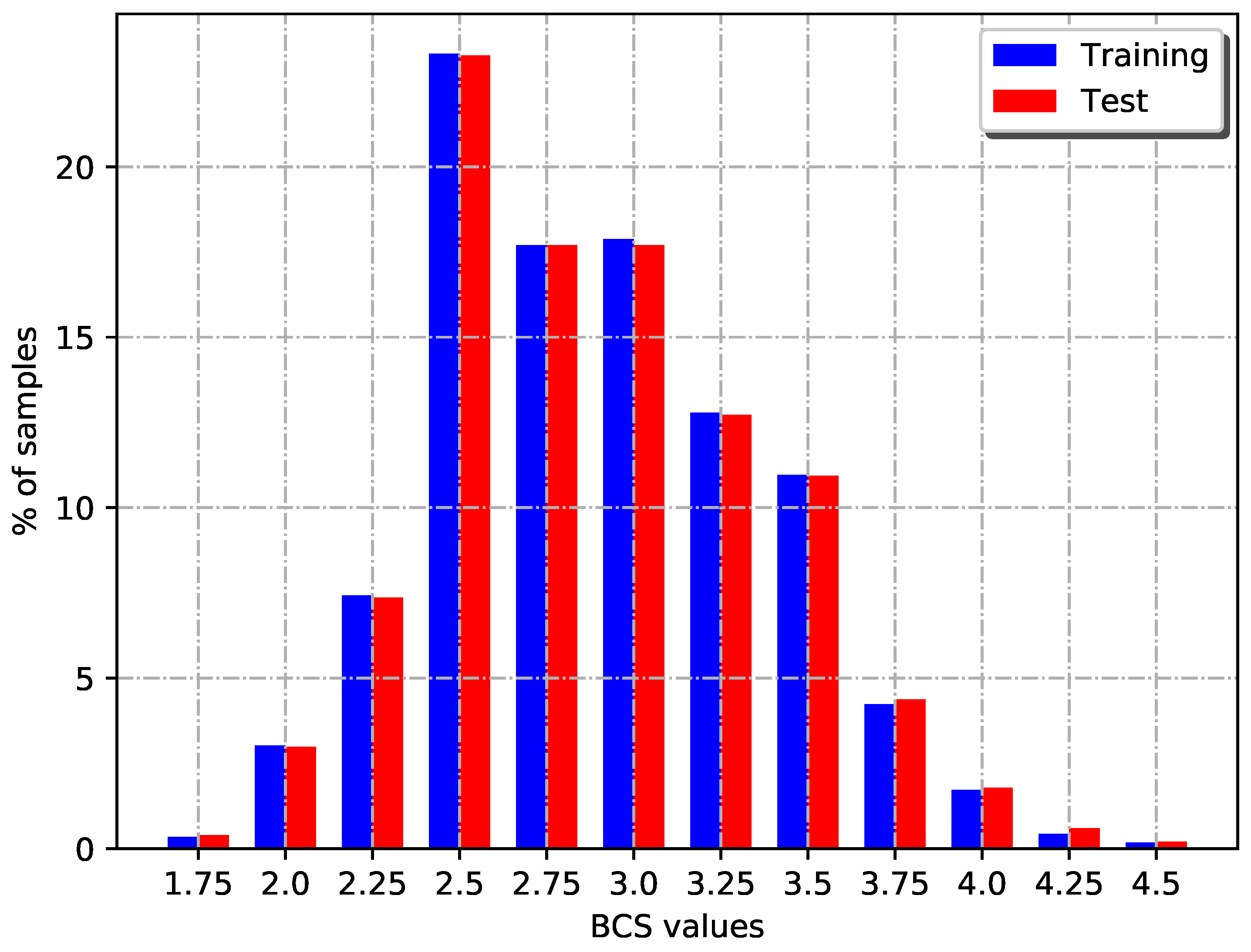
2.1. Image Collection Process and Employed Dataset
2.2. Images Preprocessing
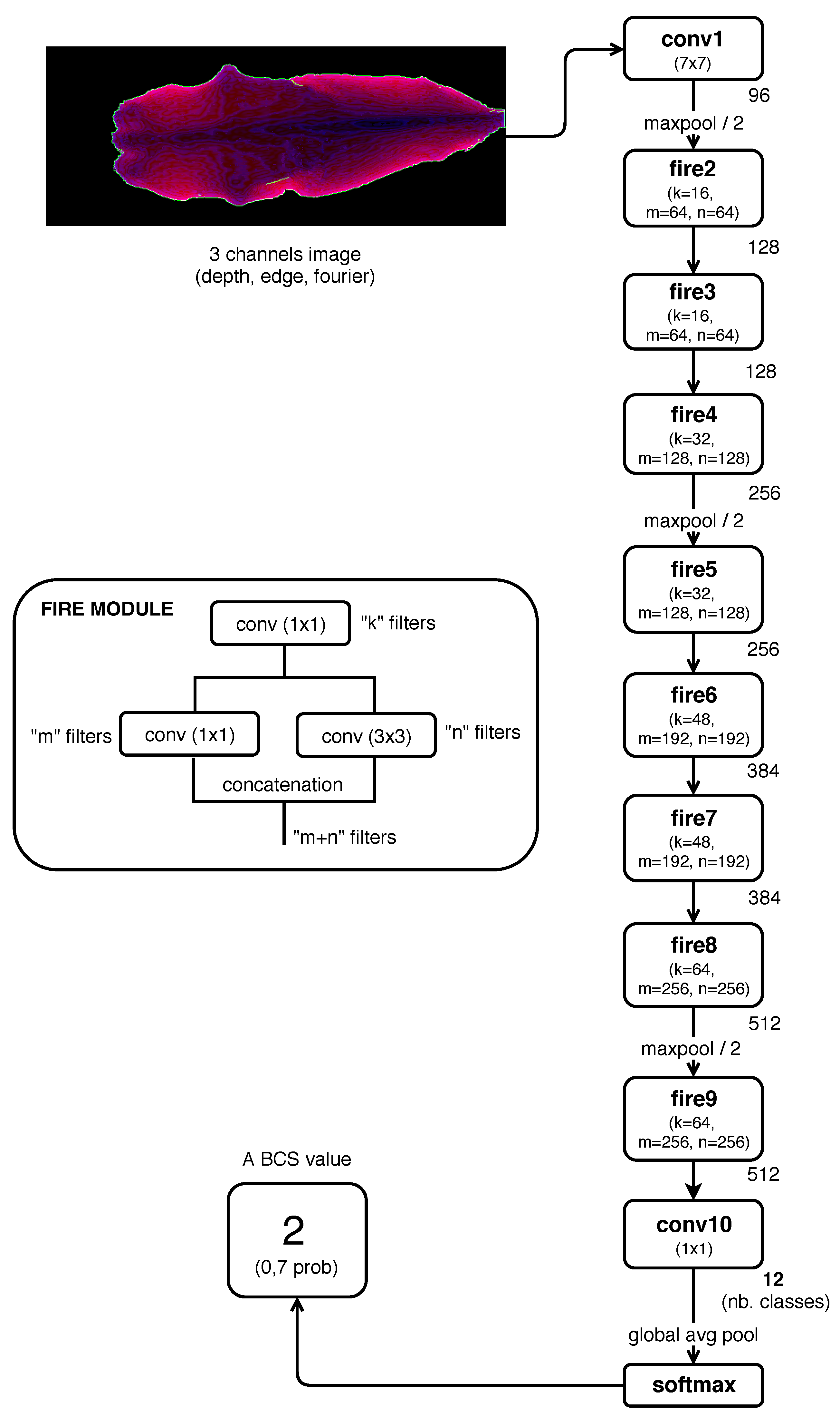
2.3. BCS Estimation Models
2.3.1. CNN Models Trained From Scratch
- Model 1: input image composed by one channel (Depth).
- Model 2: input image composed by two channel (Depth and Edge).
- Model 3: input image composed by three channel (Depth, Edge, Fourier).
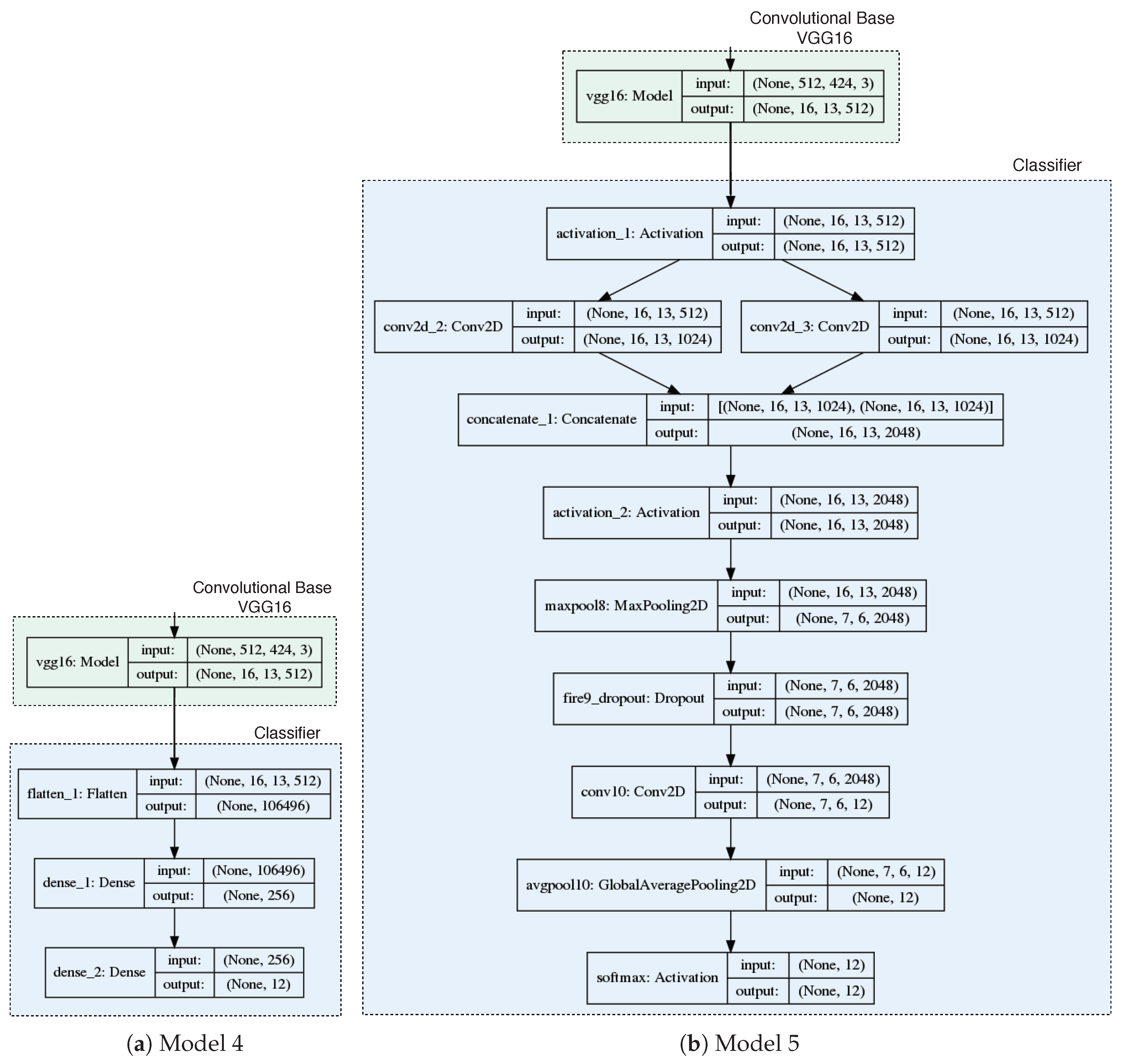
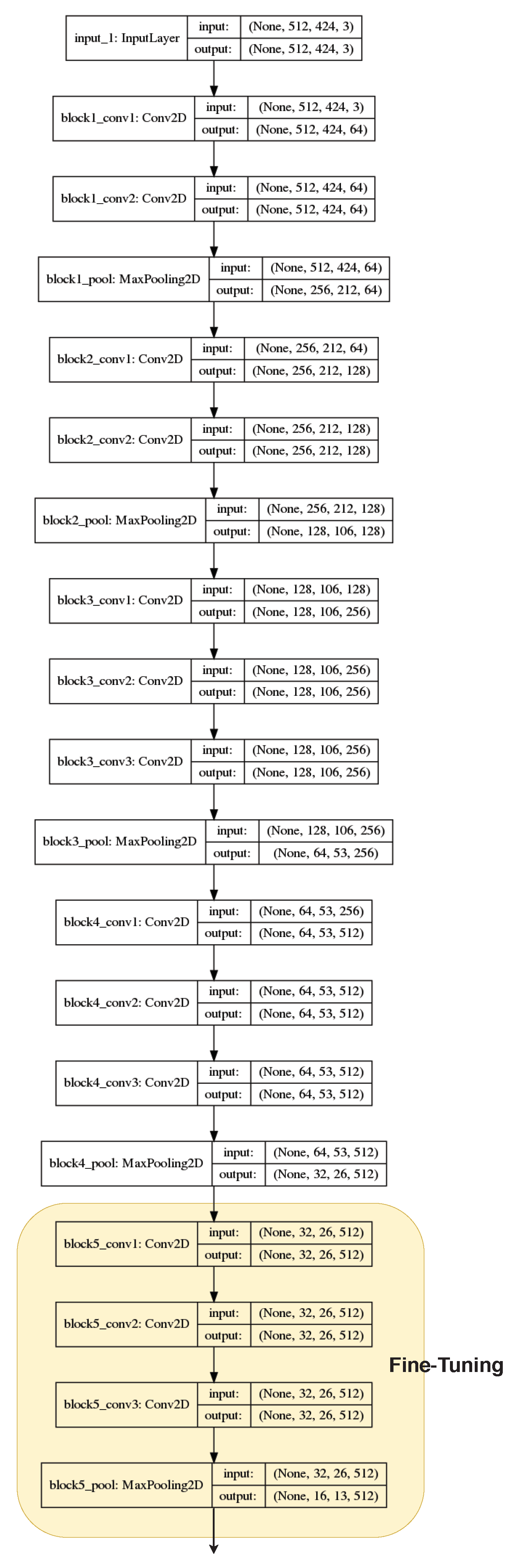
2.3.2. Transfer Learning
- Model 4: VGG16 convolutional base and fully connected classifier.
- Model 5: VGG16 convolutional base and classifier based on Fire modules.
- Model 6: fine-tuning over model 4.
- Model 7: fine-tuning over model 5.
2.3.3. Model Ensembling
2.4. Performance Evaluation
- Classification Accuracy: effectiveness of a classifier, that is the percentage of samples correctly classified. .
- Precision: ability of the classifier not to label a negative example as positive, that is the fraction of true positives (, correct predictions) from the total amount of relevant results, i.e., the sum of and (false positives). .
- Recall (a.k.a. sensitivity): ability of the classifier to find all the positive samples, that is the fraction of from the total amount of and false negatives (). .
- F1-score: one measure that combines the trade-offs of precision and recall, and outputs a single number reflecting the “goodness” of a classifier in the presence of rare classes [33]. It is the harmonic mean of precision and recall. .
3. Results and Discussion
- Model 2 (SqueezeNet 2 channels),
- Model 3 (SqueezeNet 3 channels),
- Model 6 (Fine tuning over VGG16 with a fully connected classifier),
- Model 7 (Fine tuning over VGG16 with a classifier based on Fire modules).
4. Conclusions
- Model 2: a model based on SqueezeNet with two input channels (Depth and Edge) trained from scratch;
- Model 8: an ensemble which combined the two best models (Model 2 and Model 3) with two other architecturally different models (Model 6, Model 7).
Author Contributions
Funding
Acknowledgments
Conflicts of Interest
References
- Wildman, E.; Jones, G.; Wagner, P.; Boman, R.; Troutt, H.; Lesch, T. A dairy cow body condition scoring system and its relationship to selected production characteristics. J. Dairy Sci. 1982, 65, 495–501. [Google Scholar] [CrossRef]
- Ferguson, J.; Azzaro, G.; Licitra, G. Body condition assessment using digital images. J. Dairy Sci. 2006, 89, 3833–3841. [Google Scholar] [CrossRef]
- Ferguson, J.D.; Galligan, D.T.; Thomsen, N. Principal descriptors of body condition score in Holstein cows. J. Dairy Sci. 1994, 77, 2695–2703. [Google Scholar] [CrossRef]
- Shelley, A.N. Incorporating Machine Vision in Precision Dairy Farming Technologies. Ph.D. Thesis, University of Kentucky, Lexington, KY, USA, 2016. [Google Scholar]
- Fischer, A.; Luginbühl, T.; Delattre, L.; Delouard, J.; Faverdin, P. Rear shape in 3 dimensions summarized by principal component analysis is a good predictor of body condition score in Holstein dairy cows. J. Dairy Sci. 2015, 98, 4465–4476. [Google Scholar] [CrossRef] [PubMed]
- Hansen, M.; Smith, M.; Smith, L.; Hales, I.; Forbes, D. Non-intrusive automated measurement of dairy cow body condition using 3D video. In Proceedings of the British Machine Vision Conference—Workshop of Machine Vision and Animal Behaviour, Swansea, Wales, UK, 10 September 2015; BMVA Press: Durham, England, UK, 2015; pp. 1.1–1.8. [Google Scholar]
- Bercovich, A.; Edan, Y.; Alchanatis, V.; Moallem, U.; Parmet, Y.; Honig, H.; Maltz, E.; Antler, A.; Halachmi, I. Development of an automatic cow body condition scoring using body shape signature and Fourier descriptors. J. Dairy Sci. 2013, 96, 8047–8059. [Google Scholar] [CrossRef] [PubMed]
- Halachmi, I.; Klopčič, M.; Polak, P.; Roberts, D.; Bewley, J. Automatic assessment of dairy cattle body condition score using thermal imaging. Comput. Electron. Agric. 2013, 99, 35–40. [Google Scholar] [CrossRef]
- Azzaro, G.; Caccamo, M.; Ferguson, J.; Battiato, S.; Farinella, G.; Guarnera, G.; Puglisi, G.; Petriglieri, R.; Licitra, G. Objective estimation of body condition score by modeling cow body shape from digital images. J. Dairy Sci. 2011, 94, 2126–2137. [Google Scholar] [CrossRef]
- Spoliansky, R.; Edan, Y.; Parmet, Y.; Halachmi, I. Development of automatic body condition scoring using a low-cost 3-dimensional Kinect camera. J. Dairy Sci. 2016, 99, 7714–7725. [Google Scholar] [CrossRef]
- Deng, L.; Yu, D. Deep learning: Methods and applications. Found. Trends® Signal Process 2014, 7, 197–387. [Google Scholar] [CrossRef]
- Hijazi, S.; Kumar, R.; Rowen, C. Using Convolutional Neural Networks for Image Recognition, 2015. Available online: http://site.eet-china.com/webinar/pdf/Cadence_0425_webinar_WP.pdf (accessed on 15 December 2018).
- Krizhevsky, A.; Sutskever, I.; Hinton, G.E. Imagenet classification with deep convolutional neural networks. Adv. Neural Inf. Process. Syst. 2012, 25, 1097–1105. [Google Scholar] [CrossRef]
- Szegedy, C.; Liu, W.; Jia, Y.; Sermanet, P.; Reed, S.; Anguelov, D.; Erhan, D.; Vanhoucke, V.; Rabinovich, A. Going deeper with convolutions. In Proceedings of the IEEE Conference on Computer Vision and Pattern Recognition, Boston, MA, USA, 7–12 June 2015; pp. 1–9. [Google Scholar]
- Rodríguez Alvarez, J.; Arroqui, M.; Mangudo, P.; Toloza, J.; Jatip, D.; Rodríguez, J.M.; Teyseyre, A.; Sanz, C.; Zunino, A.; Machado, C.; et al. Body condition estimation on cows from depth images using Convolutional Neural Networks. Comput. Electron. Agric. 2018, 155, 12–22. [Google Scholar] [CrossRef]
- Kamilaris, A.; Prenafeta-Boldú, F.X. Deep learning in agriculture: A survey. Comput. Electron. Agric. 2018, 147, 70–90. [Google Scholar] [CrossRef]
- Demmers, T.G.M.; Cao, Y.; Gauss, S.; Lowe, J.C.; Parsons, D.J.; Wathes, C.M. Neural predictive control of broiler chicken growth. IFAC Proc. Vol. 2010, 43, 311–316. [Google Scholar] [CrossRef]
- Demmers, T.G.M.; Gauss, S.; Wathes, C.M.; Cao, Y.; Parsons, D.J. Simultaneous monitoring and control of pig growth and ammonia emissions. In Proceedings of the Ninth International Livestock Environment Symposium (ILES IX), International Conference of Agricultural Engineering-CIGR-AgEng 2012: Agriculture and Engineering for a Healthier Life, Valencia, Spain, 8–12 July 2012. [Google Scholar]
- Santoni, M.M.; Sensuse, D.I.; Arymurthy, A.M.; Fanany, M.I. Cattle race classification using gray level co-occurrence matrix convolutional neural networks. Procedia Comput. Sci. 2015, 59, 493–502. [Google Scholar] [CrossRef]
- Pan, S.J.; Yang, Q. A survey on transfer learning. IEEE Trans. Knowl. Data Eng. 2010, 22, 1345–1359. [Google Scholar] [CrossRef]
- Canny, J. A computational approach to edge detection. IEEE Trans. Pattern Anal. Mach. Intell. 1986, PAMI-8, 679–698. [Google Scholar] [CrossRef]
- Ding, L.; Goshtasby, A. On the Canny edge detector. Pattern Recognit. 2001, 34, 721–725. [Google Scholar] [CrossRef]
- Iandola, F.N.; Han, S.; Moskewicz, M.W.; Ashraf, K.; Dally, W.J.; Keutzer, K. SqueezeNet: AlexNet-level accuracy with 50x fewer parameters and <0.5 MB model size. arXiv, 2016; arXiv:1602.07360. [Google Scholar]
- Bewley, J.; Peacock, A.; Lewis, O.; Boyce, R.; Roberts, D.; Coffey, M.; Kenyon, S.; Schutz, M. Potential for estimation of body condition scores in dairy cattle from digital images. J. Dairy Sci. 2008, 91, 3439–3453. [Google Scholar] [CrossRef]
- Salau, J.; Haas, J.; Junge, W.; Bauer, U.; Harms, J.; Bieletzki, S. Feasibility of automated body trait determination using the SR4K time-of-flight camera in cow barns. Springer Plus 2014, 3, 225. [Google Scholar] [CrossRef]
- Goodfellow, I.; Bengio, Y.; Courville, A. Deep Learning; MIT Press: Cambridge, MA, USA, 2016. [Google Scholar]
- Chollet, F. Deep Learning with Python; Manning Publications Co.: Shelter Island, NY, USA, 2017. [Google Scholar]
- Yosinski, J.; Clune, J.; Bengio, Y.; Lipson, H. How transferable are features in deep neural networks? Adv. Neural Inf. Process. Syst. 2014, 27, 3320–3328. [Google Scholar]
- Keras. 2015. Available online: https://github.com/fchollet/keras (accessed on 30 November 2018).
- Simonyan, K.; Zisserman, A. Very deep convolutional networks for large-scale image recognition. arXiv, 2014; arXiv:1409.1556. [Google Scholar]
- Stehman, S.V. Selecting and interpreting measures of thematic classification accuracy. Remote Sens. Environ. 1997, 62, 77–89. [Google Scholar] [CrossRef]
- Han, J.; Pei, J.; Kamber, M. Data Mining: Concepts and Techniques; Elsevier: Amsterdam, The Netherlands, 2011. [Google Scholar]
- Maimon, O.; Rokach, L. Data Mining and Knowledge Discovery Handbook, 2nd ed.; Springer: Berlin, Germany, 2010. [Google Scholar]
- Sokolova, M.; Lapalme, G. A systematic analysis of performance measures for classification tasks. Inf. Process. Manag. 2009, 45, 427–437. [Google Scholar] [CrossRef]
- Krukowski, M. Automatic Determination of Body Condition Score of Dairy Cows From 3D Images. Master’s Thesis, Royal Institute of Technology, School of Computer Science and Communication, Stockholm, Sweden, 2009. [Google Scholar]
- Anglart, D. Automatic Estimation of Body Weight and Body Condition Score in Dairy Cows Using 3D Imaging Technique. Master’s Thesis, Faculty of Veterinary Medicine and Animal Science, Swedish University of Agricultural Sciences, Uppsala, Sweden, 2010. [Google Scholar]


| BCS Value (Class) | Training Values Distribution | Test Values Distribution |
|---|---|---|
| 1.75 | 4 | 2 |
| 2.00 | 35 | 15 |
| 2.25 | 86 | 37 |
| 2.50 | 270 | 117 |
| 2.75 | 205 | 89 |
| 3.00 | 207 | 89 |
| 3.25 | 148 | 64 |
| 3.50 | 127 | 55 |
| 3.75 | 49 | 22 |
| 4.00 | 20 | 9 |
| 4.25 | 5 | 3 |
| 4.50 | 2 | 1 |
| Accuracy (%) | |||||||
|---|---|---|---|---|---|---|---|
| Error range | M1 | M2 | M3 | M4 | M5 | M6 | M7 |
| 0 (exact) | 30.00 | 39.56 | 35.78 | 24.45 | 31.41 | 33.40 | 30.22 |
| 0.25 | 65.21 | 81.31 | 77.13 | 60.83 | 67.39 | 66.60 | 71.37 |
| 0.50 | 89.26 | 96.82 | 95.82 | 88.67 | 89.26 | 89.46 | 91.85 |
| BCS Value | Precision (%) | Recall (%) | F1-Score (%) | ||||||||||||||||||
|---|---|---|---|---|---|---|---|---|---|---|---|---|---|---|---|---|---|---|---|---|---|
| M1 | M2 | M3 | M4 | M5 | M6 | M7 | M1 | M2 | M3 | M4 | M5 | M6 | M7 | M1 | M2 | M3 | M4 | M5 | M6 | M7 | |
| 1.75 | 0 | 0 | 0 | 0 | 0 | 0 | 0 | 0 | 0 | 0 | 0 | 0 | 0 | 0 | 0 | 0 | 0 | 0 | 0 | 0 | 0 |
| 2.00 | 50 | 0 | 33 | 0 | 0 | 0 | 100 | 7 | 0 | 13 | 0 | 0 | 0 | 7 | 12 | 0 | 19 | 0 | 0 | 0 | 12 |
| 2.25 | 0 | 32 | 33 | 25 | 33 | 44 | 37 | 0 | 27 | 14 | 8 | 3 | 19 | 27 | 0 | 29 | 19 | 12 | 5 | 26 | 31 |
| 2.50 | 36 | 47 | 43 | 41 | 39 | 39 | 47 | 64 | 51 | 51 | 30 | 63 | 66 | 44 | 46 | 49 | 47 | 34 | 49 | 49 | 45 |
| 2.75 | 33 | 35 | 29 | 21 | 26 | 32 | 25 | 17 | 46 | 27 | 28 | 25 | 22 | 49 | 22 | 40 | 28 | 24 | 25 | 26 | 33 |
| 3.00 | 21 | 39 | 30 | 21 | 29 | 19 | 24 | 20 | 42 | 40 | 26 | 19 | 13 | 10 | 20 | 40 | 34 | 23 | 23 | 16 | 14 |
| 3.25 | 20 | 30 | 38 | 14 | 22 | 27 | 21 | 28 | 25 | 33 | 27 | 25 | 14 | 31 | 24 | 27 | 35 | 19 | 24 | 19 | 25 |
| 3.50 | 34 | 43 | 42 | 33 | 27 | 32 | 31 | 42 | 45 | 45 | 29 | 45 | 67 | 29 | 37 | 44 | 44 | 31 | 34 | 43 | 30 |
| 3.75 | 25 | 43 | 38 | 36 | 60 | 40 | 33 | 5 | 45 | 27 | 18 | 14 | 27 | 5 | 8 | 44 | 32 | 24 | 22 | 32 | 8 |
| 4.00 | 0 | 0 | 14 | 0 | 0 | 0 | 0 | 0 | 0 | 11 | 0 | 0 | 0 | 0 | 0 | 0 | 12 | 0 | 0 | 0 | 0 |
| 4.25 | 0 | 0 | 0 | 0 | 0 | 0 | 0 | 0 | 0 | 0 | 0 | 0 | 0 | 0 | 0 | 0 | 0 | 0 | 0 | 0 | 0 |
| 4.50 | 0 | 0 | 0 | 0 | 0 | 0 | 0 | 0 | 0 | 0 | 0 | 0 | 0 | 0 | 0 | 0 | 0 | 0 | 0 | 0 | 0 |
| Weighted average per class | 27 | 37 | 35 | 26 | 30 | 30 | 33 | 30 | 40 | 36 | 24 | 31 | 33 | 30 | 26 | 38 | 35 | 24 | 28 | 29 | 28 |
| Unweighted average per class | 18 | 23 | 25 | 16 | 20 | 19 | 24 | 15 | 23 | 22 | 14 | 16 | 19 | 17 | 14 | 23 | 23 | 14 | 15 | 18 | 17 |
| BCS Value | Precision (%) | Recall (%) | F1-Score (%) | ||||||||||||||||||
|---|---|---|---|---|---|---|---|---|---|---|---|---|---|---|---|---|---|---|---|---|---|
| M1 | M2 | M3 | M4 | M5 | M6 | M7 | M1 | M2 | M3 | M4 | M5 | M6 | M7 | M1 | M2 | M3 | M4 | M5 | M6 | M7 | |
| 1.75 | 0 | 0 | 100 | 0 | 0 | 0 | 0 | 0 | 0 | 100 | 0 | 0 | 0 | 0 | 0 | 0 | 100 | 0 | 0 | 0 | 0 |
| 2.00 | 50 | 100 | 80 | 0 | 0 | 100 | 100 | 7 | 40 | 27 | 0 | 0 | 13 | 13 | 12 | 57 | 40 | 0 | 0 | 24 | 24 |
| 2.25 | 100 | 85 | 94 | 82 | 100 | 91 | 76 | 68 | 76 | 81 | 49 | 73 | 84 | 70 | 81 | 80 | 87 | 61 | 84 | 87 | 73 |
| 2.50 | 56 | 82 | 77 | 76 | 65 | 62 | 81 | 69 | 87 | 76 | 59 | 81 | 81 | 90 | 62 | 84 | 77 | 66 | 72 | 70 | 85 |
| 2.75 | 86 | 78 | 82 | 60 | 72 | 81 | 59 | 82 | 89 | 90 | 65 | 79 | 79 | 83 | 84 | 83 | 86 | 62 | 75 | 80 | 69 |
| 3.00 | 54 | 76 | 64 | 58 | 69 | 58 | 86 | 58 | 75 | 76 | 80 | 55 | 38 | 74 | 56 | 76 | 69 | 67 | 61 | 46 | 80 |
| 3.25 | 56 | 87 | 83 | 41 | 62 | 80 | 54 | 59 | 81 | 78 | 64 | 62 | 64 | 53 | 58 | 84 | 81 | 50 | 62 | 71 | 54 |
| 3.50 | 64 | 82 | 71 | 67 | 53 | 46 | 69 | 76 | 84 | 71 | 71 | 75 | 78 | 75 | 69 | 83 | 71 | 69 | 62 | 58 | 72 |
| 3.75 | 100 | 81 | 90 | 89 | 94 | 74 | 91 | 59 | 100 | 82 | 36 | 73 | 77 | 45 | 74 | 90 | 86 | 52 | 82 | 76 | 61 |
| 4.00 | 67 | 100 | 88 | 100 | 100 | 100 | 100 | 22 | 78 | 78 | 22 | 11 | 22 | 11 | 33 | 88 | 82 | 36 | 20 | 36 | 20 |
| 4.25 | 100 | 0 | 100 | 0 | 0 | 0 | 0 | 33 | 0 | 33 | 0 | 0 | 0 | 0 | 50 | 0 | 50 | 0 | 0 | 0 | 0 |
| 4.50 | 0 | 0 | 0 | 0 | 0 | 0 | 0 | 0 | 0 | 0 | 0 | 0 | 0 | 0 | 0 | 0 | 0 | 0 | 0 | 0 | 0 |
| Weighted average per class | 67 | 81 | 78 | 63 | 67 | 69 | 73 | 65 | 81 | 77 | 61 | 67 | 67 | 71 | 65 | 81 | 77 | 60 | 66 | 65 | 70 |
| Unweighted average per class | 61 | 64 | 77 | 48 | 51 | 58 | 60 | 45 | 59 | 66 | 37 | 42 | 45 | 43 | 48 | 60 | 69 | 39 | 43 | 46 | 45 |
| BCS Value | Precision (%) | Recall (%) | F1-Score (%) | ||||||||||||||||||
|---|---|---|---|---|---|---|---|---|---|---|---|---|---|---|---|---|---|---|---|---|---|
| M1 | M2 | M3 | M4 | M5 | M6 | M7 | M1 | M2 | M3 | M4 | M5 | M6 | M7 | M1 | M2 | M3 | M4 | M5 | M6 | M7 | |
| 1.75 | 0 | 100 | 100 | 100 | 0 | 100 | 100 | 0 | 100 | 100 | 50 | 0 | 100 | 100 | 0 | 100 | 100 | 67 | 0 | 100 | 100 |
| 2.00 | 100 | 100 | 100 | 100 | 100 | 100 | 100 | 93 | 87 | 100 | 40 | 87 | 87 | 60 | 97 | 93 | 100 | 57 | 93 | 93 | 75 |
| 2.25 | 100 | 95 | 97 | 100 | 100 | 100 | 90 | 73 | 98 | 95 | 78 | 84 | 89 | 95 | 84 | 96 | 96 | 88 | 91 | 94 | 92 |
| 2.50 | 84 | 98 | 97 | 94 | 89 | 88 | 97 | 90 | 98 | 97 | 87 | 91 | 92 | 96 | 87 | 98 | 97 | 91 | 90 | 90 | 97 |
| 2.75 | 100 | 96 | 98 | 90 | 93 | 96 | 85 | 93 | 97 | 96 | 96 | 89 | 84 | 96 | 97 | 96 | 97 | 93 | 91 | 90 | 90 |
| 3.00 | 91 | 99 | 97 | 91 | 95 | 95 | 99 | 99 | 98 | 98 | 100 | 100 | 98 | 98 | 95 | 98 | 97 | 95 | 97 | 96 | 98 |
| 3.25 | 81 | 97 | 95 | 73 | 83 | 95 | 87 | 75 | 97 | 95 | 95 | 89 | 84 | 97 | 78 | 97 | 95 | 82 | 86 | 89 | 92 |
| 3.50 | 81 | 96 | 90 | 83 | 73 | 68 | 85 | 98 | 96 | 95 | 89 | 85 | 91 | 80 | 89 | 96 | 92 | 86 | 79 | 78 | 82 |
| 3.75 | 100 | 88 | 91 | 100 | 95 | 83 | 95 | 100 | 100 | 95 | 95 | 91 | 91 | 95 | 100 | 94 | 93 | 98 | 93 | 87 | 95 |
| 4.00 | 88 | 100 | 100 | 100 | 100 | 100 | 100 | 78 | 100 | 100 | 33 | 78 | 89 | 56 | 82 | 100 | 100 | 50 | 88 | 94 | 71 |
| 4.25 | 100 | 100 | 100 | 0 | 0 | 0 | 0 | 33 | 67 | 33 | 0 | 0 | 0 | 0 | 50 | 80 | 50 | 0 | 0 | 0 | 0 |
| 4.50 | 0 | 0 | 0 | 0 | 0 | 0 | 0 | 0 | 0 | 0 | 0 | 0 | 0 | 0 | 0 | 0 | 0 | 0 | 0 | 0 | |
| Weighted average per class | 89 | 97 | 96 | 89 | 89 | 90 | 91 | 89 | 97 | 96 | 89 | 89 | 89 | 92 | 89 | 97 | 96 | 88 | 89 | 89 | 91 |
| Unweighted average per class | 77 | 89 | 89 | 78 | 69 | 77 | 78 | 69 | 86 | 84 | 64 | 66 | 75 | 73 | 71 | 87 | 85 | 67 | 67 | 76 | 74 |
| M2 | M3 | M6 | M7 | M8 (Ensemble) | ||
|---|---|---|---|---|---|---|
| Accuracy(%) Error Range | 0 (exact) | 39.56 | 35.78 | 33.40 | 30.22 | 41.15 |
| 0.25 | 81.31 | 77.13 | 66.60 | 71.37 | 81.51 | |
| 0.50 | 96.82 | 95.82 | 89.46 | 91.85 | 97.42 | |
| Weighted predictions models | 0.5 | 0.3 | 0.1 | 0.1 | ||
| Error Range | Krukowski (2009) | Anglart (2010) | Bercovich et al. (2013) | Shelley (2016) | Spoliansky et al. (2016) | Rodríguez Alvarez et al. (2018) | Model 2 SqueezeNet (2 Channels) | Model 8 Ensemble |
|---|---|---|---|---|---|---|---|---|
| 0.25 | 20% | 69% | 43% | 71.35% | 74% | 78% | 81% | 82% |
| 0.50 | 46% | 95% | 72% | 93.91% | 91% | 94% | 96% | 97% |
© 2019 by the authors. Licensee MDPI, Basel, Switzerland. This article is an open access article distributed under the terms and conditions of the Creative Commons Attribution (CC BY) license (http://creativecommons.org/licenses/by/4.0/).
Share and Cite
Rodríguez Alvarez, J.; Arroqui, M.; Mangudo, P.; Toloza, J.; Jatip, D.; Rodriguez, J.M.; Teyseyre, A.; Sanz, C.; Zunino, A.; Machado, C.; et al. Estimating Body Condition Score in Dairy Cows From Depth Images Using Convolutional Neural Networks, Transfer Learning and Model Ensembling Techniques. Agronomy 2019, 9, 90. https://doi.org/10.3390/agronomy9020090
Rodríguez Alvarez J, Arroqui M, Mangudo P, Toloza J, Jatip D, Rodriguez JM, Teyseyre A, Sanz C, Zunino A, Machado C, et al. Estimating Body Condition Score in Dairy Cows From Depth Images Using Convolutional Neural Networks, Transfer Learning and Model Ensembling Techniques. Agronomy. 2019; 9(2):90. https://doi.org/10.3390/agronomy9020090
Chicago/Turabian StyleRodríguez Alvarez, Juan, Mauricio Arroqui, Pablo Mangudo, Juan Toloza, Daniel Jatip, Juan M. Rodriguez, Alfredo Teyseyre, Carlos Sanz, Alejandro Zunino, Claudio Machado, and et al. 2019. "Estimating Body Condition Score in Dairy Cows From Depth Images Using Convolutional Neural Networks, Transfer Learning and Model Ensembling Techniques" Agronomy 9, no. 2: 90. https://doi.org/10.3390/agronomy9020090
APA StyleRodríguez Alvarez, J., Arroqui, M., Mangudo, P., Toloza, J., Jatip, D., Rodriguez, J. M., Teyseyre, A., Sanz, C., Zunino, A., Machado, C., & Mateos, C. (2019). Estimating Body Condition Score in Dairy Cows From Depth Images Using Convolutional Neural Networks, Transfer Learning and Model Ensembling Techniques. Agronomy, 9(2), 90. https://doi.org/10.3390/agronomy9020090