Article

Estimating Crop Transpiration of Soybean under Different Irrigation Treatments Using Thermal Infrared Remote Sensing Imagery

1
Center for Agricultural Water Research in China, China Agricultural University, Beijing 100083, China
2
CSIRO Land and Water Flagship, Canberra ACT 2601, Australia
*
Author to whom correspondence should be addressed.
Agronomy 2019, 9(1), 8; https://doi.org/10.3390/agronomy9010008
Submission received: 17 October 2018 / Revised: 19 December 2018 / Accepted: 21 December 2018 / Published: 26 December 2018
(This article belongs to the Special Issue Increasing Agricultural Water Productivity in a Changing Environment)

Abstract

:
Temporal and spatial resolution of satellite images are coarse and cannot provide the real-time, meter-scale resolution monitoring required in many applications, such as precision agriculture. Since high resolution thermal infrared data provide one means to observe canopy temperature variance, we developed an algorithm (three-temperature model, 3T) to estimate transpiration rate at meter-scale pixels and detected transpiration variation for soybean under different upper irrigation limits: No irrigation, 35% of field capacity (FC), 55% of FC, and 75% of FC, denoted as W0, W1, W2, and W3, respectively. The spatial patterns of the transpiration rate indicated that heterogeneity is common in farmland. Transpiration rates in the wet treatment (i.e., W3) were consistently higher than that in the dry treatment (i.e., W0). Transpiration rates reached peak values at around 12:30–14:30 and most of values showed that W3 > W2 > W1 > W0, with 0.91 mm/h, 0.89 mm/h, 0.79 mm/h, and 0.62 mm/h during the reproductive period, respectively. In general, the transpiration rate of soybean increased with increasing irrigation quantities. With a higher irrigation total, soil water content increased gradually, and then the transpiration rate increased. Although land surface temperature decreased by only 8.57 K (Kelvin), 6.33 K, and 5.47 K, respectively, the transpiration rate increased by 78%, 60%, and 40%, respectively, for the W3, W2, and W1 treatment compared with the W0 treatment. The magnitude of transpiration change is greater than that of canopy temperature, but both parameters are strongly interrelated with each other through a non-linear correlation. Heterogeneity of canopy leaf temperature and transpiration is mainly due to physical and biological interactions. Understanding transpiration rate and canopy temperature heterogeneity under different irrigation treatments can not only help in scheduling irrigation, but also in enhancing water utilization efficiency in irrigated agriculture. The real-time monitoring of crop transpiration at meter-scale is of great importance for large irrigation systems, especially for precision irrigation, and will have great application prospects in the near future.

1. Introduction

Agriculture in water stressed and arid environments is maintained through irrigation. In order to effectively manage water resources in these areas, it is necessary to optimize the use of irrigation water by reducing water losses [1]. Evapotranspiration (ET, soil evaporation (E) + vegetation transpiration (T)) is a critical component in the water cycle and the energy flow between the land surface and atmosphere, and it plays an important role in hydrology and ecology. Evapotranspiration accounts for approximately 60% of annual land precipitation on a global basis [2] and about 80–90% of consumptive water use for crop production in semi-arid regions [3]. For irrigated agriculture, the amount of water to be irrigated needs to be determined based on actual transpiration. Hence, it is essential to estimate how much water is transpired by a crop for better allocation of water resources and improving water-use efficiency in the irrigated agriculture.
However, it is not easy to estimate actual crop transpiration because it varies as it is affected not only by micrometeorological factors but also by stomatal aperture. A number of researchers in several fields such as remote sensing (RS), geography, hydrology, ecology, and agriculture have been studying evapotranspiration [4,5,6,7,8,9,10,11]. The conventional field-based evapotranspiration measurement techniques (i.e., eddy covariance, Bowen ratio, weighing lysimeter, stem sap flow gauge) are constrained to relatively a small scale compared with remote sensing technology. With the development of remote sensing technology, different methods have been proposed to estimate evapotranspiration through satellite remote sensing, which have proven to be useful for estimating ET at the regional and global scales [12,13,14]. From remote sensing estimation, ET can be separated pixel by pixel. Although remote sensing-based methods have significant advantages over conventional methods in obtaining large-scale distributed data at various spatial and temporal resolutions, the complexity of these methods varies [15]. A number of algorithms such as the Surface Energy Balance Algorithm for Land (SEBAL) [16] and the Atmosphere-Land Exchange Inverse (ALEXI) model [17] rely on meteorological variables such as wind speed, air temperature, and vapor pressure. Satellite based remote sensing ET is limited by an infrequency of observations as a result of cloudiness and orbital schedules. Besides, satellite images do not provide meter-scale resolution data required in many applications, such as ecosystem restoration and precision agriculture [18]. Additionally, the low temporal resolution and coarse spatial resolution of satellite imaging might introduce significant error due to subpixel heterogeneity [19]. Consequently, it is difficult to quantitatively characterize differences at meter pixels in farmland.
Following the development of thermal infrared imaging techniques, there are increasing applications for remote sensing. With its high resolution, airborne remote sensing can bridge the gaps between ground-based measurement and satellite remote sensing estimation [20], and this technique has been applied to estimate soil evaporation (E) at the field-scale [21]. Egea et al. [22] assessed a crop water stress index derived from aerial thermal imaging and infrared thermometry in super-high-density olive orchards. Banerjee et al. [23] used thermal imaging of a wheat crop canopy to estimate leaf area index under different moisture stress conditions at the 1 m scale. The thermal imaging technique is mature for high-resolution applications and has been widely used for evapotranspiration estimation. However, most remote sensing ET algorithms include some parameters with large spatial-temporal heterogeneity and difficulty in remote sensing inversion, such as aerodynamic and surface resistances [24]. Ershadi et al. [24] assessed the impact of parameterization choice on model performance, where a number of commonly used formulations for aerodynamic and surface resistances were substituted into the different formulations in their studies. Qiu et al. [25] developed a three-temperature model (3T model) to estimate evapotranspiration and its partition, where the required input parameters to estimate transpiration were net radiation, surface temperature, and air temperature [26,27]. Various studies showed that the 3T model could accurately estimate evapotranspiration and its partition under different conditions [28,29,30,31,32]. Tian et al. [33] estimated transpiration from 16 types of typical vegetation in the upper and middle reaches of the Heihe River Basin in Northwestern China using this method and showed that the 3T model is not only simple to use, but also accurate. However, in the previous studies based on the 3T model, net radiation was mainly estimated using some empirical parameters, which could introduce some uncertainty. With this empirical estimation, the differences in crop transpiration under different irrigation treatments at meter pixels in farmland are not quantitatively characterized.
Compared with previous studies based on 3T models, the 3T model used in this study not only has the following strength advantages: Pixel-by-pixel calculation, high spatial-temporal resolution, fewer input parameters, and simplicity to use, but also overcomes the problem mentioned above by observing net radiation. This will further simplify the application and improve the accuracy of the model. In addition, we have high data frequency for a long time period. The objectives of this research were to (1) determine and quantify the difference of crop transpiration of soybean under different irrigation treatments at meter pixels in an arid region; and (2) investigate the heterogeneity of canopy temperature and transpiration of soybean under different irrigation treatments, which would be beneficial for irrigation management.

2. Materials and Methods

2.1. Experimental Site

The experiment was conducted at Shiyanghe Experimental Station for Water-saving in Agriculture and Ecology, China Agricultural University, located in Wuwei City, Gansu province of northwest China (37°52′ N, 102°50′ E, altitude 1581 m, Figure 1). The experimental site has a typical continental climate, with a mean annual temperature of 7.8 °C, and annual precipitation of 164 mm. The mean annual pan evapotranspiration is about 2000 mm, with an arid index of 15–25. The average annual sunshine duration is 3000 h with 150 frost free days. The groundwater table is 40–50 m below the ground surface. The soil texture is sand loam, with a mean dry bulk density of 1.40 g cm−3 and a mean volumetric soil water content at field capacity of 0.30 cm3 cm−3.

2.2. Field Measurements

The field experiments were conducted during the reproductive stage of soybean in 2017. The soybeans were sowed by the way of mulch-covered hole sowing with three replications in randomly distributed plots of 3 m × 6 m. The plant to plant distance was 15 cm and row to row distance was 50 cm. We chose the local soybean variety Longhuang No.2 as the research object, and four upper irrigation limits (UIL) were designed under mulched drip irrigation. They were no irrigation, 35% of field capacity (FC), 55% of FC, and 75% of FC, which were set as W0, W1, W2, and W3, respectively. The soybeans were irrigated about every ten days, and the lower irrigation limits (LIL) were the average soil water content of 0–100 cm soil layer one day before the next irrigation, which was determined by a gravimetric method after collecting the soil samples from every 20 cm layer through soil drills. During our experiment, soybeans were irrigated on 28 July and 7 August, and the depth of the designed moisting soil layer was 100 cm. The relevant irrigation parameters during the experiment were shown in Table 1.
The high-resolution ground based thermal infrared remote sensing data were taken with the infrared thermal imager (Fluke IR Flex Cam TiX620, Fluke Crop., Everett, WA, USA). The measuring wave-length of the thermal camera was 7.5–14 µm, and its resolution was 640 × 480 pixels, with a sensitivity of 0.05 °C and an accuracy of ± 2 °C. The distance between the crop and the camera was about 2 m, and the angle between the canopy and the camera was about 45°. Field observation was carried out from 22 July to 18 August, 2017. The thermal images were taken every two hours from 8:30 to 18:30 on each clear sunny day, each image was taken three times and the best quality images were selected for the study. As transpiration usually constitutes the larger portion of evapotranspiration in arid regions, we only concentrated on transpiration in this research. To estimate transpiration with the 3T model, in addition to the canopy temperature obtained from the thermal imager, air temperature was collected at the nearby automatic meteorological station (Hobo, Onset Computer Corp., Bourne, MA, USA) which was approximately 100 m from the soybean field and calculated and stored 15 min averages, and net solar radiation of the soybean and imitation soybean were continuously measured by the CNR4 four-component radiometer (Kipp & Zonen, Delft, The Netherlands) of the Bowen ratio system which was about 10 m from the soybean field.

2.3. Estimation of Transpiration Based on 3T Model

The foundation of the 3T model is a surface energy balance equation that can be described as:
λET = RnGH
where, λET is the latent heat flux, λ is the latent heat of vaporization with 2.45 × 10⁶ W m−2 mm−1 and ET is the evapotranspiration (ET = E + T). Rn is the net radiation, G is the soil heat flux, and H is the sensible heat flux. All units are in W m−2. It should be emphasized that we only focus on the energy balance of the canopy using Equation (1). In the canopy covered area, the incident radiation is intercepted by the canopy so that partitioning of energy at the soil surface is relatively insignificant. In addition, with the closure of the canopy and the surface coverage, evaporation from canopy shadowed soil is generally very low, so it is reasonable to ignore G on a daily basis. Therefore, the energy balance at the vegetation surface can be expressed as:
λT = Rn,cHc
where, λT is the latent heat flux of the vegetation; Rn,c and Hc are, respectively, the surface net radiation and the sensible heat flux of the vegetation; all units are the same as above. Hc referred to in Equation (2) can be calculated by the following equations [34,35]:
H c   =   ρ C p ( T c T a ) r a
where, ρ is the air density in kg m−3, Cp is the specific heat at constant pressure (MJ kg−1 °C−1), Tc is the surface temperature of the canopy (K), Ta is the air temperature (K), and ra is the aerodynamic resistance (s m−1), the diffusion resistance of the air layer.
Aerodynamic resistance (ra) is affected by a number of factors and cannot be remotely measured. In order to solve this problem, we introduced a green leaf-shaped piece of paper near the observed vegetation as an imitation canopy, which has zero transpiration (λT = 0). As there is no significant change in the atmospheric conditions around the imitation canopy, we assume that the aerodynamic resistance and air temperature of the surrounding vegetation are the same as those of the imitation canopy (rara,cp, TaTa,cp) [34,36]. For imitation leaf, λT = 0, according to Equation (2), Rn,cp = Hc. Combining Equations (2) and (3), we find that:
  R n , c p   =   H c = ρ C p ( T c T a ) r a
then ra can be calculated by Equation (5):
r a   =   ρ C p ( T c p T a ) R n , c p
where, Tcp and Rn;cp are, respectively, the surface temperature and net radiation of the imitation canopy. The subscripts ‘‘a’’, ‘‘c’’, and ‘‘cp’’ represent the air, canopy, and the imitation canopy. By combining Equations (2), (3), and (5), λT can be estimated as:
λ T = R n , c R n , c p T c T a T c p T a .
where all units are the same as above, and for this meter-scale research, we set Rn,c = Rn,cp, and then Equation (6) can be simplified as:
λ T = R n , c . ( T c , p T c T c , p T a )
In addition to Tc and Tcp obtained by thermal infrared camera, air temperature was measured by the nearby HOBO automatic meteorological station, and net solar radiation was continuously measured by the CNR4 four-component radiometer of the Bowen ratio system. A more detailed description of the model can be found in Qiu et al. [26,27,34], Xiong et al. [37] and Tian et al. [33]. As the major input parameters were canopy temperature, the imitation canopy temperature, air temperature, and net solar radiation, and all the parameters were easy to obtain, the 3T model has been proven to be able to estimate the transpiration of various plants [26,34,36,37,38,39], and was also well simulated in the adjacent inland river basin Heihe Basin which has the similar climate [33]. Given the structure of the article and the good performance of the model in former research, details such as model validation are not highlighted in this research.

3. Results

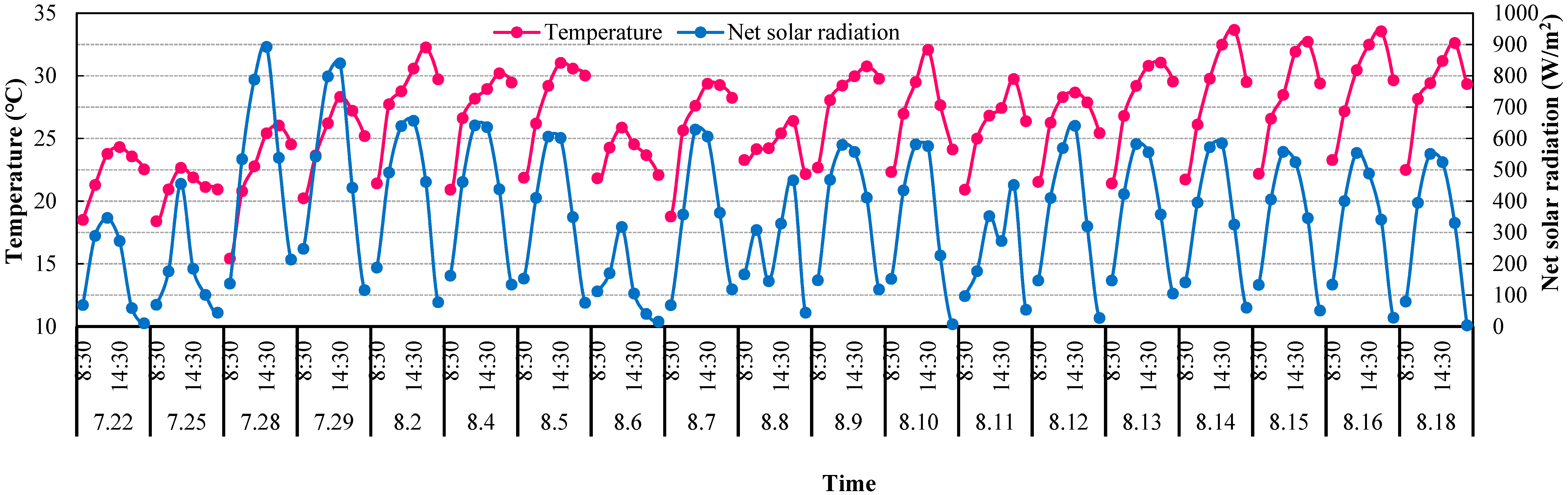
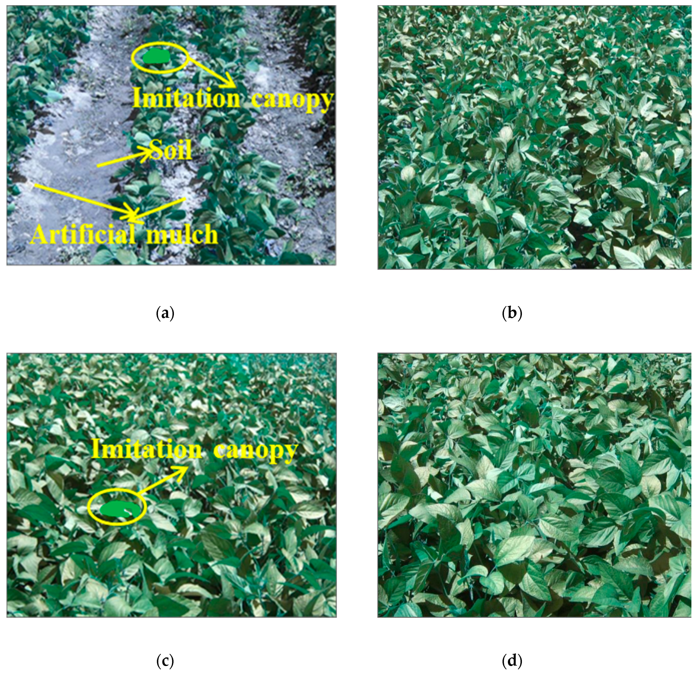
3.1. Results of Field Measurements

During the daytime, the air temperature of the experimental site experienced a single peak curve change. As shown in Figure 2, at 8:30, the air temperature was relatively low (about 15–20 °C). After that, the temperature began to rise; it reached its peak (about 23–34 °C) at about 14:30 or 16:30, and then it gradually declined until evening. The temperatures on the 22 July and 25 July were relatively low. Net solar radiation had the same pattern as air temperature. Around 08:30, the value was positive (around 10 W m−2—Watt m−2: the solar radiation energy that incidents vertically on per square meter in one second.); it reached the peak (300–900 Wm−2) at 12:30 or 14:30, and then it declined in the afternoon and became negative in the evening. The radiation values for the 22 July and 6 August were relatively low.
Visible-light images (Figure 3) and high-resolution thermal infrared remote sensing images (Figure 4) of soybean under four different irrigation treatments for the growth period of 2017 were obtained, respectively. A total of 1368 thermal infrared images were obtained. Given the limited space available, the highest transpiration rate was at about 12:30, so only the images obtained at this moment were shown in Figure 3, Figure 4 and Figure 5. From these 640 × 480 pixel resolution images, soil, crops, and other things can be clearly identified. Combined with the supervised classification methods of ENVI 4.8 software (ENVI Visual Information Solutions, Boulder, CO, USA), crop, soil, and other landscape characteristics were classified, but we only chose the crop regions as the regions of interest, and then the estimated transpiration in these pixels were counted.

3.2. Monitoring Spatial Change of Land Surface Temperature and Transpiration Rate

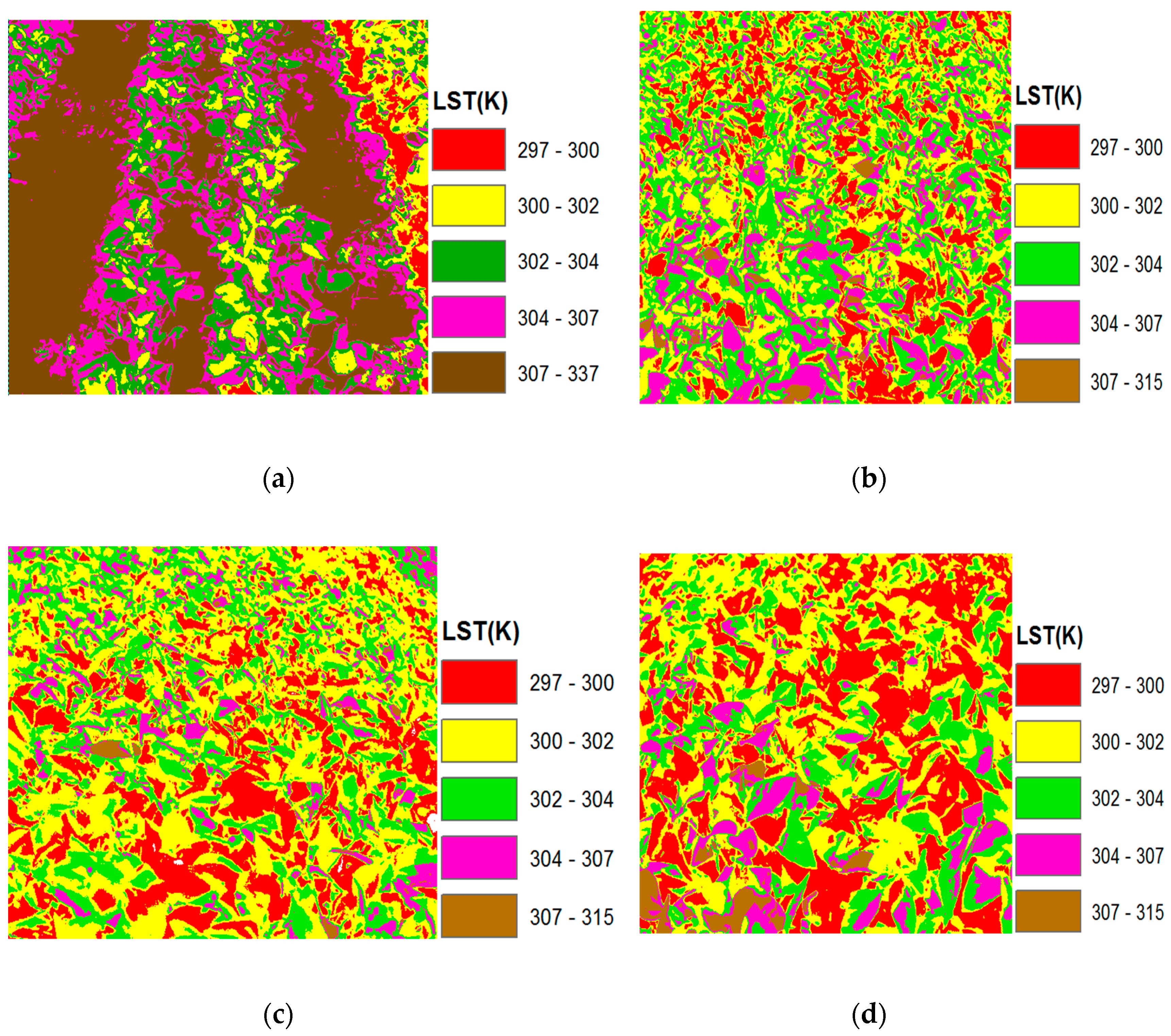
3.2.1. Spatial Change of Land Surface Temperature

From Figure 4 we can clearly see that the land surface temperature (LST) not only experienced large changes for soybean under different irrigation treatments, but also had large spatial variation for soybean in the same treatment (especially the changes that occurred between the soil and canopy in Figure 4a). As shown in Figure 4, with increasing irrigation totals, the amount of canopy with a low temperature increased, and the average temperatures of soybeans under the treatment of W0, W1, W2, and W3 decreased gradually, which were 306.88 K, 303.16 K, 301.93 K, and 300.13 K, respectively. With the increased irrigation totals, the surface temperatures at 12:30 on August 5th decreased by 6.75 K, 4.95 K, and 3.72 K, respectively, for the treatment of W3, W2, and W1, compared with the treatment of W0. For soybeans treated with the same irrigation amount, the temperature of the soil for W0 treatment was the highest, at about 337 K, however, the canopy temperature was relatively low, about 40 K lower than the soil temperature. The canopy temperature of the other three treatments also changed greatly, for example, some canopies ranged from 297 K to 300 K, and some other canopies were 307–315 K, which indicated that the heterogeneity from land surface was very common and this method could clearly distinguish this kind of difference at the meter scale.

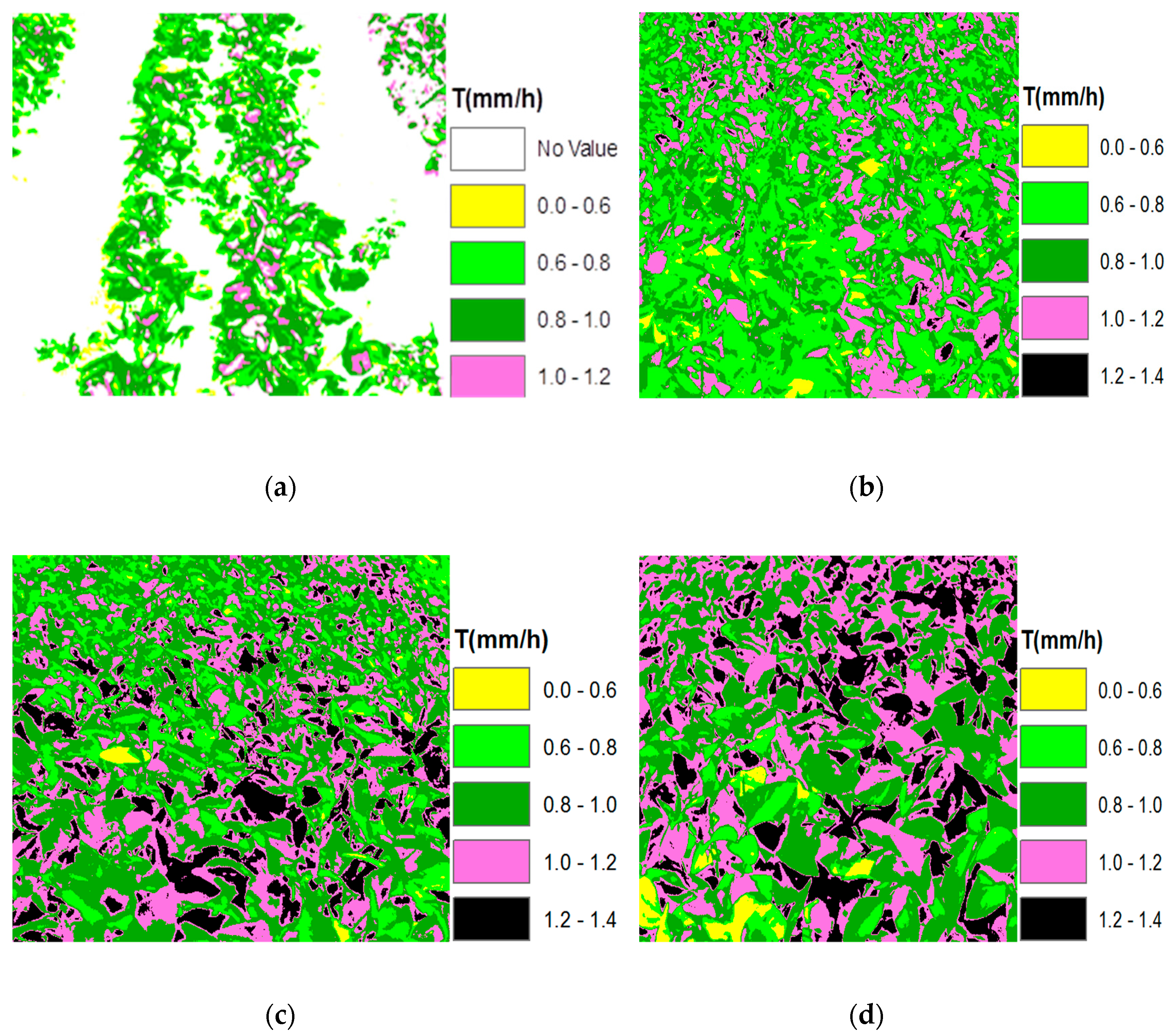
3.2.2. Spatial Change of Transpiration Rates

The instant spatial distribution of transpiration rates at 12:30 of the soybeans with four different irrigation treatments (W0, W1, W2, W3) were presented in Figure 5. Results demonstrated that, like the spatial distribution of LST, transpiration rate had also experienced great spatial changes, and the distribution of transpiration rates was not uniform. For example, transpiration was 0.0–0.6 mm/h in some canopies, and 1.0–1.2 mm/h in some others canopies at 12:30, which also indicated that heterogeneity was very common. However, compared with the spatial distribution of LST, it is found that the canopy with high temperature had a small transpiration rate. Additionally, transpiration rates in the wet treatment (i.e., W3) were consistently higher than that in the dry treatment (i.e., W0). The corresponding mean transpiration rate for the treatment of W0, W1, W2, and W3 were 0.79 mm/h, 0.84 mm/h, 0.87 mm/h, and 1.01 mm/h, respectively, at 12:30 on 5 August, 2017. With the higher irrigation amount, soil water content increased gradually, and then the transpiration rate increased. With the increased irrigation total, transpiration increased by 0.22 mm/h, 0.08 mm/h, and 0.05 mm/h, respectively, for the treatment of W3, W2, and W1, compared with the treatment of W0.

3.3. Monitoring Temporal Change of Land Surface Temperature and Transpiration Rates

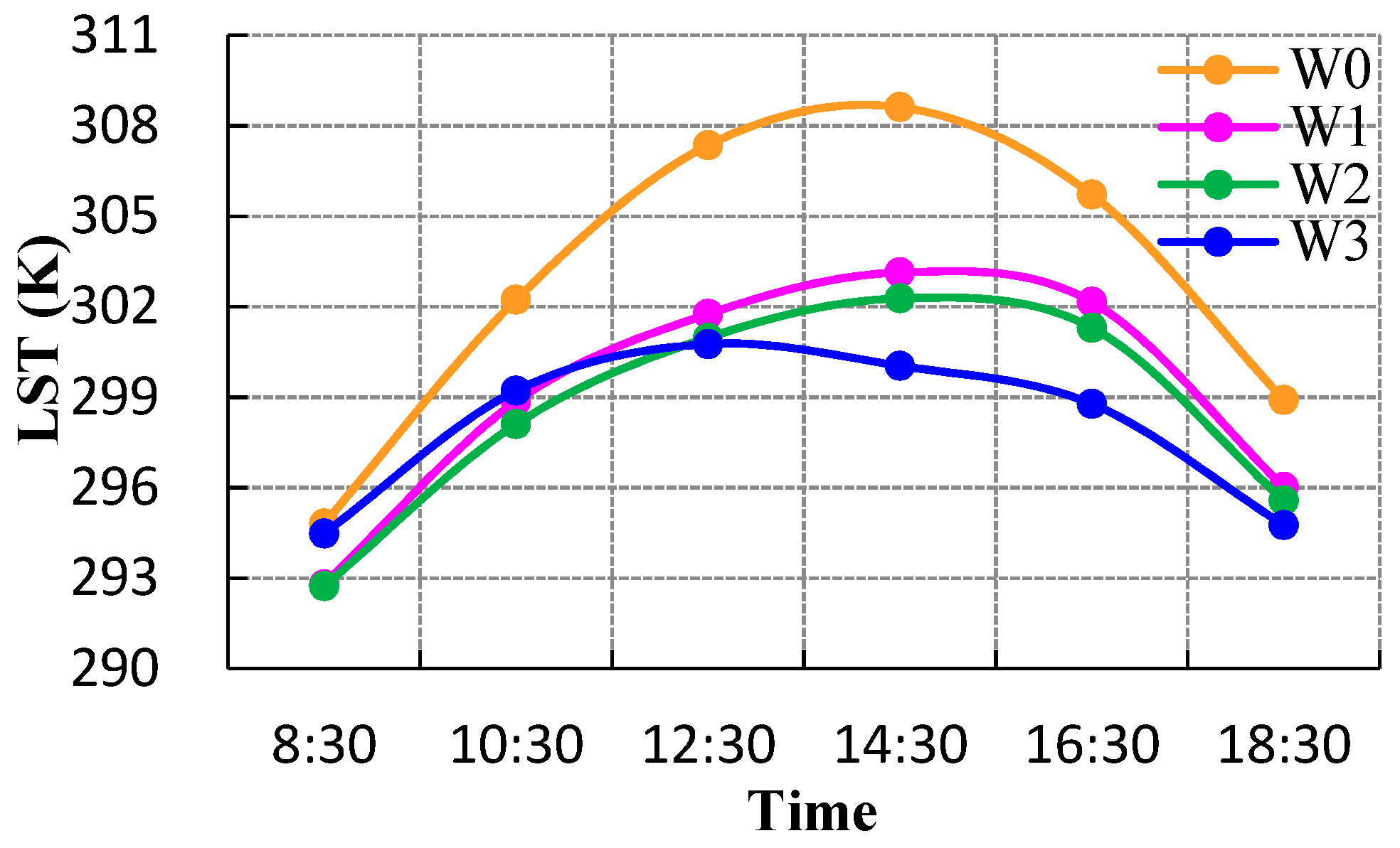
3.3.1. Temporal Change of Land Surface Temperature

Figure 6 displays the temporal changes of LST for soybean during the experimental period. Changes of daily LST showed that most of them experienced a single peak curve change, which was similar to the changes of temperature and net solar radiation, that is, starting in the morning and increasing rapidly, and then declining toward the evening. The LST reached peak values at around 12:30–14:30 and most of the values showed that W3 < W2 < W1 < W0. The midday LST of four irrigation treatments ranged from 292 K to 320 K, the value was not only affected by meteorological conditions, but also related to irrigation amount. The maximum peak values for the treatment of W0, W1, W2, and W3 occurred at around 14:30 and were detected as 320.01 K, 313.64 K, 311.62 K, and 307.30 K, respectively. The canopy temperature decreased after irrigation and increased gradually with water consumption.
From the daytime variation of the average LST during the reproductive period in Figure 7, it is clearly shown that the average LST of soybean under different irrigation treatments has a single peak curve, with peak values around 14:30, and the peak values were about 308.61 K, 303.14 K, 302.28 K, and 300.04 K, respectively, in the W0, W1, W2, and W3 treatment. Obviously, the mean LST experienced great decrease with the increase of irrigation, and the canopy temperature difference for the treatment of W3 and W0 was around 8.57 K.

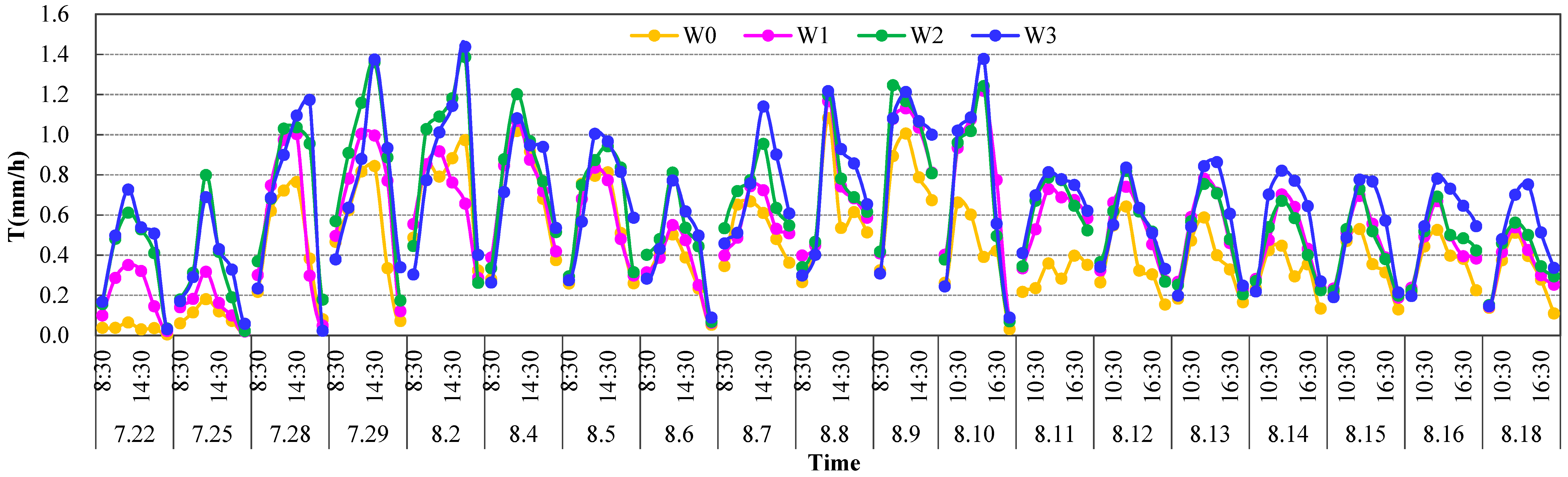
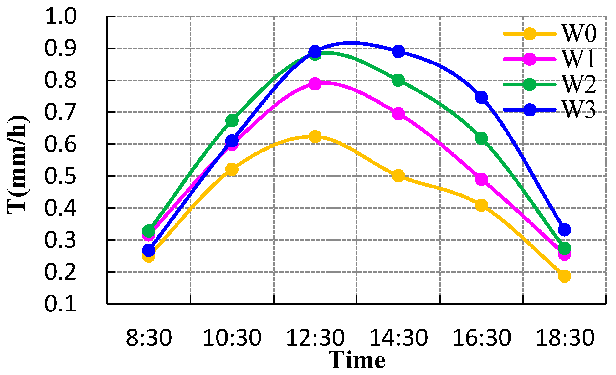
3.3.2. Temporal Change of Transpiration Rates

Figure 8 displays the temporal change of transpiration for soybean during the experimental period. The changing trend of daily transpiration of soybean treated with different irrigation quantities was basically the same as that of the corresponding LST. The time when transpiration rate reached its peak was also basically the same as that of LST, which was about 12:30–14:30, but the changing law of transpiration rate especially for peak value was opposite to the LST, most of which were W3 > W2 > W1 > W0. The peak value and peak shape differ depending on the amount of water through irrigation and the irrigation time. The transpiration rate reached peak value within 1–3 days after irrigation and then had a slight decline as time passed, which indicated that a lag effect existed in transpiration. The peak transpiration of soybean under four irrigation treatments ranged between 0.07 mm/h and 1.44 mm/h, and the maximum peak values for W0, W1, W2, and W3 occurred at about 14:30 and were detected as 1.05 mm/h, 1.17 mm/h, 1.37 mm/h, and 1.44 mm/h, respectively. The transpiration rate in W0 treatment occasionally appeared as a “midday depression” phenomenon, and the daily changing trend was a bimodal curve.
From the daytime variation of the average transpiration rate during the reproductive period in Figure 9, we can draw the same conclusion as before, that is, the transpiration rate showed that W3 > W2 > W1 > W0, and in general, the transpiration rate of soybean increased alongside the increase of irrigation amount. Another difference from LST was that the average transpiration peaks of soybeans with W0, W1, W2, and W3 treatment occurred at about 12:30 with 0.62 mm/h, 0.79 mm/h, 0.89 mm/h, and 0.91 mm/h, respectively, which was earlier than that of LST. The average transpiration rates for W0, W1, W2, and W3 treatment at 14:30 were 0.50 mm/h, 0.70 mm/h, 0.80 mm/h, and 0.89 mm/h, respectively. We can find that average transpiration rates for the W3, W2, and W1 treatment increased by 0.39 mm/h, 0.30 mm/h, and 0.20 mm/h compared with W0 treatment at 14:30 during the experiment. This means it increased by 78%, 60% and 40%, respectively, while the LSTs decreased by 8.57 K, 6.33 K, and 5.47 K, correspondingly. These results indicated that irrigation can significantly change the transpiration rate of soybean.

4. Discussion

Detecting how much water is transpired by a crop canopy is critical for better allocating water resources and for scheduling irrigation [40,41,42]. The conventional field-based transpiration measurement techniques and most remotely sensed models rely heavily on ground-based auxiliary measurements, and many parameters are hardly obtained accurately [15]. Furthermore, because of the low temporal and coarse spatial resolution of satellite images [18], it is difficult to quantitatively characterize the heterogeneous differences in farmland. As a result of these issues, we used a simple method to estimate crop transpiration rate at meter pixels. This method has three advantages. The first is that it eliminates aerodynamic resistance by introducing an imitation leaf temperature Tcp, which heavily reduces some of the uncertainties. The second advantage is that it requires a minimum amount of inputs which are easy to obtain. The necessary inputs are Tc, Tcp, Ta, and net radiation. All the inputs can be directly measured or estimated from other measure data for ground-based measurements, so it has great potential for use in developing countries where ground information is scarce. The third is that the transpiration rate is calculated pixel by pixel. Remotely sensed surface temperature can provide a measure of the surface from a few cm2 with a hand-held thermometer to about several km2 from certain satellites [43], so this method provides a bridge between large-scale and point observation.
Comparing and contrasting the spatial variations of canopy temperatures and transpiration rates, we found that heterogeneity was prevalent among them, and the instant transpiration rates at 12:30 on 5 August for soybean (Figure 5) were negatively correlated with canopy temperatures (Figure 4). For example, transpirations in W1 treatment were 0.0–0.6 mm/h in some canopies, and 1.0–1.2 mm/h in some others, while corresponding canopy temperatures were 307–315 K and 297–300 K, respectively. Transpiration rates in the wet treatment (i.e., W3) were consistently higher than that in the dry treatment (i.e., W0), but for canopy temperature, the changing law was opposite. With the increase of total irrigation from W0 to W3, the LSTs at 12:30 on 5 August decreased by 1.80 K, 3.03 K, and 6.75 K in turn, while the transpiration rates increased by 0.05 mm/h, 0.08mm/h, and 0.22 mm/h, respectively. With the higher irrigation amount, soil water content increased gradually, and then the transpiration rate increased, which led to a reduction in the canopy temperature, and produced a cooling effect. Bonfils and Lobell [44] compared temperature trends in irrigated areas with those in nearby non-irrigated areas, and also showed that irrigation decreased summertime maximum temperature by 2–3 K, or irrigation induced a cooling of 1 K in maximum growing season temperatures in irrigated areas. Kueppers et al. [45] found that irrigated crops cooled an irrigated area by 3.7 K in August and 1.6 K year around. Differences in the magnitude of the irrigation cooling effect between different studies can be partly explained by differences in how irrigation was modeled, and how much water they added through irrigation. These indicated that irrigation can significantly change the field micro-climate and promote transpiration of soybean.
In fact, according to many other studies [46,47,48,49,50,51,52,53,54], we can conclude that heterogeneity of canopy temperature mainly results from physical and biological interactions, which are affected by climatic conditions (such as wind, temperature, vapor-pressure deficit, relative humidity, long wave radiation, and the angle of radiation incident on the leaf surface), environmental conditions (soil temperature at 2 cm depth, soil moisture, adjacent objects, and solar height), canopy structure complexity (leaf inclination distribution frequency, size, shape, and position), canopy parameters (canopy albedo, emissivity, and stomatal resistance) and ecosystem functions (evapotranspiration and photosynthesis). Among these studies, the result of Smith and Carter [47] showed that the temperatures of needle-leaf were closer to air temperature than that of broad leaves, and needle leaves usually remained within 4–8 K of air temperature, whereas Jones [48] reported that sunlit broadleaves might be 10–15 K higher than air temperatures. Kim et al. [49] found that leaf temperature was non-linearly related to air temperature, and the relationship between mean leaf temperature and net ecosystem exchange during the afternoon was closer than that of air temperature, which was mainly driven by the strong correlation between tissue temperature and photosynthesis and respiration. Han et al. [50] proposed that sunlit leaves received more direct radiation than shaded leaves of the canopy, and had higher temperature than that of shaded leaves, and Tan et al. [53] also found that the temperature at the top of canopy was always higher than that in the middle of canopy, indicating the effect of shading on temperature within the canopy.
The temporal transpiration and LST changes under different irrigation treatments (Figure 6, Figure 7, Figure 8 and Figure 9) for soybean are almost all single peak curves, and they reached the peak values at around 12:30–14:30. Most of the transpiration rates were shown as W3 > W2 > W1 > W0, with average peak values of 0.89 mm/h, 0.80 mm/h, 0.70 mm/h, and 0.50 mm/h at 14:30 during the experiment, respectively; and most LSTs were shown as W0 > W1 > W2 > W3, with the corresponding average peak values of 308.61 K, 303.14 K, 302.28 K, and 300.04 K, respectively. That means that although LSTs decreased by only 8.57 K, 6.33 K, and 5.47 K, respectively, the transpiration rates increased by 78%, 60%, and 40%, respectively, for the W3, W2, and W1 treatment compared with W0 treatment. In addition to the comprehensive effects of the various factors mentioned above, the biggest influencing factor for transpiration rate in this study is the irrigation amount. Under the same background, with the increase of irrigation amount, crops rarely suffer from water stress and grow better (such as having a denser canopy), so they have higher canopy transpiration rates and latent heat fluxes which finally resulted in more heat lost, therefore, the transpiration cooling effect is obvious, and then presented lower canopy temperatures. Irrigation can promote crop transpiration, and the magnitude of transpiration change is greater than that in canopy temperature, accounting for the lag effect.
To some extent, variations of transpiration rates directly reflect the ability of crops to regulate water loss and their ability to adapt to dry or wet environments [33], which is closely related to canopy temperature. Canopy temperature can be used to calculate a crop water stress index and stomatal conductance index, which can detect drought stress and support irrigation scheduling [41,42,54]. Therefore, evaluation of transpiration and canopy temperature is of great significance for monitoring plant water status and scheduling irrigation and understanding the crop transpiration and temperature under different irrigation schedules. Using high-resolution thermal infrared remote sensing data can not only help for scheduling irrigation, but also in enhancing water utilization efficiency of irrigated agriculture. Additionally, the spatial and temporal resolution is coarser in satellite imagery [18], which means this kind of real-time monitoring of crop transpiration at meter scale is of great importance for large irrigation systems, especially for precision irrigation, and will have great application prospects in the future.

5. Conclusions

This paper introduced a method (3T model + high resolution thermal infrared remote sensing) to estimate transpiration rates of plants at meter-scale pixels. We applied the method to soybean under different irrigation treatments. It was found that: (1) Heterogeneity was very common for transpiration rate, its distribution was not uniform at meter-scale, and the temporal variation of transpiration for the soybean under different irrigation treatments mostly had a single peak around 12:30–14:30, and most values showed that W3 > W2 > W1 > W0, that is, the increase of irrigation water increased transpiration rate, and the transpiration rate in the wet treatment was consistently higher than that in the dry treatment. (2) Although LSTs decreased by only 8.57 K, 6.33 K, and 5.47 K, respectively, the transpiration rate increased by 78%, 60%, and 40%, respectively, for the W3, W2, and W1 treatment compared with the W0 treatment. The magnitude of transpiration change is greater than that of the canopy temperature, both parameters are strongly interrelated with each other, but they are non-linearly correlated. (3) Heterogeneity of canopy leaf temperature is mainly due to physical and biological interactions, which are affected by climatic conditions, environmental conditions, canopy structure complexity, canopy parameters, and ecosystem functions. Under the same background, with the increase of irrigation amount, the transpiration cooling effect is obvious, which then presents a lower canopy temperature.

Author Contributions

Conceptualization, F.T.; Methodology, M.H. (Mengjie Hou) and F.T.; Software, M.H. (Mengjie Hou); Validation, Y.Y. and T.D.; Resources, M.H. (Mengsi Huang) and S.L.; Data Curation, M.H. (Mengjie Hou) and F.T.; Writing—Original Draft Preparation, M.H. (Mengjie Hou); Writing—Review & Editing, F.T. and L.Z.; Visualization, M.H. (Mengjie Hou); Supervision, L.Z.; Project Administration, F.T.; Funding Acquisition, F.T.

Funding

We acknowledge the financial support from the National Natural Science Foundation of China -Youth Science Foundation Project (41601015), the National Natural Science Foundation of China-Major Program (51790534), and the Basic Research Fund Project from China Agricultural University (2018QC132).

Acknowledgments

Thanks to Meng Duan and Jia Li for providing radiation and meteorological data. We also thank the fruitful comments by the editors and anonymous reviewers.

Conflicts of Interest

The authors declare no conflict of interest.

References

  1. Gaur, N.; Mohanty, B.P.; Kefauver, S.C. Effect of observation scale on remote sensing based estimates of evapotranspiration in a semi-arid row cropped orchard environment. Precis. Agric. 2017, 18, 762–778. [Google Scholar] [CrossRef]
  2. Oki, T.; Kanae, S. Global hydrological cycles and world water resources. Science 2006, 313, 1068–1072. [Google Scholar] [CrossRef] [PubMed]
  3. Zang, C.F.; Liu, J.G.; Van, D.V.M.; Kraxner, F. Assessment of spatial and temporal patterns of green and blue water flows under natural conditions in inland river basins in Northwest China. Hydrol. Earth Syst. Sci. 2012, 16, 1–12. [Google Scholar] [CrossRef]
  4. Farahani, H.J.; Bausch, W.C. Performance of Evapotranspiration Models for Maize Bare Soil to Closed Canopy. Trans. ASABE 1995, 38, 1049–1059. [Google Scholar] [CrossRef]
  5. Rana, G.; Katerji, N.; Mastrorilli, M.; Moujabber, M.E. A model for predicting actual evapotranspiration under soil water stress in a Mediterranean region. Theor. Appl. Climatol. 1997, 56, 45–55. [Google Scholar] [CrossRef]
  6. Sun, Z.G.; Wang, Q.X.; Matsushita, B.; Fukushima, T.; Ouyang, Z.; Watanabe, M. Development of a simple remote sensing Evapotranspiration model (Sim-Re SET): Algorithm and model test. J. Hydrol. 2009, 376, 476–485. [Google Scholar] [CrossRef]
  7. Elhaddad, A.; Garcia, L.A.; Chávez, J.L. Using a surface energy balance model to calculate spatially distributed actual evapotranspiration. J. Irrig. Drain. Eng. 2011, 137, 17–26. [Google Scholar] [CrossRef]
  8. Chen, Y.Y.; Chu, C.R.; Li, M.H. A gap-filling model for eddy covariance latent heat flux: Estimating evapotranspiration of a subtropical seasonal evergreen broad-leaved forest as an example. J. Hydrol. 2012, 468–469, 101–110. [Google Scholar] [CrossRef]
  9. Liu, M.L.; Adam, J.C.; Hamlet, A.F. Spatial-temporal variations of evapotranspiration and runoff/precipitation ratios responding to the changing climate in the Pacific Northwest during 1921–2006. J. Geophys. Res. D. Atmos. JGR 2013, 118, 380–394. [Google Scholar] [CrossRef]
  10. Tang, R.L.; Li, Z.L. An improved constant evaporative fraction method for estimating daily evapotranspiration from remotely sensed instantaneous observations. Geophys. Res. Lett. 2017, 44, 2319–2326. [Google Scholar] [CrossRef]
  11. Cong, Z.T.; Shen, Q.N.; Zhou, L.; Sun, T.; Liu, J.H. Evapotranspiration estimation considering anthropogenic heat based on remote sensing in urban area. Sci. China Earth Sci. 2017, 60, 659–671. [Google Scholar] [CrossRef]
  12. Wagle, P.; Bhattarai, N.; Gowda, P.H.; Kakani, V.G. Performance of five surface energy balance models for estimating daily evapotranspiration in high biomass sorghum. ISPRS J. Photogramm. Remote Sens. 2017, 128, 192–203. [Google Scholar] [CrossRef]
  13. Knipper, K.; Hogue, T.; Scott, R.; Franz, K. Evapotranspiration Estimates Derived Using Multi-Platform Remote Sensing in a Semiarid Region. Remote Sens. 2017, 9, 184. [Google Scholar] [CrossRef]
  14. Abrishamkar, M.; Ahmadi, A. Evapotranspiration Estimation Using Remote Sensing Technology Based on SEBAL Algorithm. Iran. J. Sci. Technol. Trans. Civ. Eng. 2017, 41, 65–76. [Google Scholar] [CrossRef]
  15. Courault, D.; Seguin, B.; Olioso, A. Review on estimation of evapotranspiration from remote sensing data: From empirical to numerical modeling approaches. Irrig. Drain. Syst. 2005, 19, 223–249. [Google Scholar] [CrossRef]
  16. Bastiaanssen, W.G.M.; Menenti, M.; Feddes, R.A.; Holtslag, A.A.M. A remote sensing surface energy balance algorithm for land (SEBAL) 1. Formulation. J. Hydrol. 1998, 212–213, 198–212. [Google Scholar] [CrossRef]
  17. Anderson, M.C.; Norman, J.M.; Mecikalski, J.R.; Otkin, J.A.; Kustas, W.P. A climatological study of evapotranspiration and moisture stress across the continental United States based on thermal remote sensing: 1. Model formulation. J. Geophys. Res. Atmos. 2007, 112, D10117. [Google Scholar] [CrossRef]
  18. Loheide, S.P.; Gorelick, S.M. A local-scale, high-resolution evapotranspiration mapping algorithm (ETMA) with hydroecological applications at riparian meadow restoration sites. Remote Sens. Environ. 2005, 98, 182–200. [Google Scholar] [CrossRef]
  19. Kustas, W.P.; Norman, J.M. Evaluating the Effects of Subpixel Heterogeneity on Pixel Average Fluxes. Remote Sens. Environ. 2000, 74, 327–342. [Google Scholar] [CrossRef]
  20. Qiu, G.Y.; Zhao, M. Remotely monitoring evaporation rate and soil water status using thermal imaging and “three-temperatures model (3T Model)” under field-scale conditions. J. Environ. Monit. 2010, 12, 716–723. [Google Scholar] [CrossRef] [PubMed]
  21. Qiu, G.Y.; Ben-Asher, J. Experimental Determination of Soil Evaporation Stages with Soil Surface Temperature. Soil Phys. 2010, 74, 13–22. [Google Scholar] [CrossRef]
  22. Egea, G.; Padilla-Díaz, C.M.; Martinez-Guanter, J.; Fernández, J.E.; Pérez-Ruiz, M. Assessing a crop water stress index derived from aerial thermal imaging and infrared thermometry in super-high density olive orchards. Agric. Water Manag. 2017, 187, 210–221. [Google Scholar] [CrossRef] [Green Version]
  23. Banerjee, K.; Krishnan, P.; Mridha, N. Application of thermal imaging of wheat crop canopy to estimate leaf area index under different moisture stress conditions. Biosyst. Eng. 2018, 166, 13–27. [Google Scholar] [CrossRef]
  24. Ershadia, A.; McCabea, M.F.; Evansb, J.P.; Woodc, E.F. Impact of model structure and parameterization on Penman-Monteith type evaporation models. J. Hydrol. 2015, 525, 521–535. [Google Scholar] [CrossRef]
  25. Qiu, G.Y. A New Method for Estimation of Evapotranspiration. Ph.D. Thesis, The United Graduate School of Agriculture Science, Tttori University, Tttori, Japan, 1996; p. 197. [Google Scholar]
  26. Qiu, G.Y.; Momii, K.; Yano, T. Estimation of plant transpiration by imitation leaf temperature. I. Theoretical consideration and field verification. Trans. Jpn. Soc. Irrig. Drain. Reclam. Eng. 1996, 64, 401–410. [Google Scholar]
  27. Qiu, G.Y.; Yano, T.; Momii, K. An improved methodology to measure evaporation from bare soil based on comparison of surface temperature with a dry soil. J. Hydrol. 1998, 210, 93–105. [Google Scholar] [CrossRef]
  28. Qiu, G.Y.; Shi, P.J.; Wang, L.M. Theoretical analysis of a soil evaporation transfer coefficient. Remote Sens. Environ. 2006, 101, 390–398. [Google Scholar] [CrossRef]
  29. Xiong, Y.J.; Qiu, G.Y.; Chen, X.H.; Zhao, S.H.; Tian, F. Estimation of evapotranspiration using three-temperature model based on MODIS data. J. Remote Sens. 2012, 16, 969–985. [Google Scholar]
  30. Tian, F.; Qiu, G.Y.; Yang, Y.H.; Lv, Y.H.; Xiong, Y.J. Estimation of evapotranspiration and its partition based on an extended three-temperature model and MODIS products. J. Hydrol. 2013, 498, 210–220. [Google Scholar] [CrossRef]
  31. Xiong, Y.J.; Qiu, G.Y. Simplifying the revised three-temperature model for remotely estimating regional evapotranspiration and its application to a semi-arid steppe. Int. J. Remote Sens. 2014, 35, 2003–2027. [Google Scholar]
  32. Qiu, G.Y.; Li, C.; Yan, C.H. Characteristics of soil evaporation: Plant transpiration and water budget of Nitraria dune in the arid Northwest China. Agric. For. Meteorol. 2015, 203, 107–117. [Google Scholar] [CrossRef]
  33. Tian, F.; Qiu, G.Y.; Lü, Y.H.; Yang, Y.H.; Xiong, Y.J. Use of high-resolution thermal infrared remote sensing and “three-temperature model” for transpiration monitoring in arid inland river catchment. J. Hydrol. 2014, 515, 307–315. [Google Scholar] [CrossRef]
  34. Qiu, G.Y.; Momii, K.; Yano, T.; Lascano, R.J. Experiment verification of a mechanistic model to partition evaporation into soil water and plant evaporation. Agric. For. Meteorol. 1999, 93, 79–93. [Google Scholar] [CrossRef]
  35. Jackson, R.D. Canopy temperature and crop water stress. In Advances in Irrigation; Hillel, D., Ed.; Academic Press: New York, NY, USA, 1982; Volume 1, pp. 43–85. [Google Scholar]
  36. Yu, X.H.; Yang, Y.J.; Tan, S.L.; Li, R.L.; Qin, H.P.; Qiu, G.Y. Evapotranspiration and its cooling effect of urban green roof. Chin. J. Environ. Eng. 2017, 11, 5333–5340. (In Chinese) [Google Scholar]
  37. Xiong, Y.J.; Qiu, G.Y. Estimation of evapotranspiration using remotely sensed land surface temperature and the revised three-temperature model. Int. J. Remote Sens. 2011, 32, 5853–5874. [Google Scholar] [CrossRef]
  38. Wang, Y.Q.; Xiong, Y.J.; Qiu, G.Y.; Zhang, Q.T. Is scale really a challenge in evapotranspiration estimation? A multi-scale study in the Heihe oasis using thermal remote sensing and the three-temperature model. Agric. For. Meteorol. 2016, 230–231, 128–141. [Google Scholar] [CrossRef]
  39. Xiong, Y.J.; Zhao, S.; Tian, F.; Qiu, G.Y. An evapotranspiration product for arid regions based on the three-temperature model and thermal remote sensing. J. Hydrol. 2015, 530, 392–404. [Google Scholar] [CrossRef] [Green Version]
  40. Kadam, S.A.; Gorantiwar, S.D.; Das, S.N.; Joshi, A.K. Crop Evapotranspiration Estimation for Wheat (Triticum aestivum L.) Using Remote Sensing Data in Semi-Arid Region of Maharashtra. J. Indian Soc. Remote Sens. 2017, 45, 297–305. [Google Scholar] [CrossRef]
  41. Ćosić, M.; Stričević, R.; Djurović, N.; Lipovac, A.; Bogdan, I.; Pavlović, M. Effects of irrigation regime and application of kaolin on canopy temperatures of sweet pepper and tomato. Sci. Horticult. 2018, 238, 23–31. [Google Scholar] [CrossRef]
  42. Maes, W.H.; Steppe, K. Estimating evapotranspiration and drought stress with ground-based thermal remote sensing in agriculture: A review. J. Exp. Bot. 2012, 63, 4671–4712. [Google Scholar] [CrossRef] [PubMed]
  43. Li, Z.L.; Tang, R.L.; Wan, Z.M.; Bi, Y.Y.; Zhou, C.H.; Tang, B.H.; Yan, G.J.; Zhang, X.Y. A review of current methodologies for regional evapotranspiration estimation from remotely sensed data. Sensors 2009, 9, 3801–3853. [Google Scholar] [CrossRef] [PubMed]
  44. Bonfils, C.; Lobell, D.B. Empirical evidence for a recent slowdown in irrigation-induced cooling. Proc. Natl. Acad. Sci. USA 2007, 104, 13582–13587. [Google Scholar] [CrossRef] [Green Version]
  45. Kueppers, L.M.; Snyder, M.A.; Sloan1, L.C. Irrigation cooling effect: Regional climate forcing by land-use change. Geophys. Res. Lett. 2007, 34. [Google Scholar] [CrossRef] [Green Version]
  46. Francois, C.; Ottle, C.; Prevot, L. Analytical parameterization of canopy directional emissivity and directional radiance in the thermal infrared. Application on the retrieval of soil and foliage temperatures using two directional measurements. Int. J. Remote Sens. 1997, 18, 2587–2621. [Google Scholar] [CrossRef]
  47. Smith, W.K.; Carter, G.A. Shoot structural effects on needle temperatures and photosynthesis in conifers. Am. J. Bot. 1988, 75, 496–500. [Google Scholar] [CrossRef]
  48. Jones, H.G. Application of thermal imaging and infrared sensing in plant physiology and ecophysiology. Adv. Bot. Res. 2004, 41, 107–163. [Google Scholar]
  49. Kim, Y.; Still, C.J.; Hanson, C.V.; Kwon, H.; Greer, B.T.; Law, B.E. Canopy skin temperature variations in relation to climate, soil temperature, and carbon flux at a ponderosa pine forest in central Oregon. Agric. For. Meteorol. 2016, 226–227, 161–173. [Google Scholar] [CrossRef]
  50. Han, M.; Zhang, H.H.; DeJonge, K.C.; Comas, L.H.; Trouta, T.J. Estimating maize water stress by standard deviation of canopy temperature in thermal imagery. Agric. Water Manag. 2016, 177, 400–409. [Google Scholar] [CrossRef]
  51. Song, Q.H.; Deng, Y.; Zhang, Y.P.; Deng, X.B.; Lin, Y.X.; Zhou, L.G.; Fei, X.H.; Sha, L.Q.; Liu, Y.T.; Zhou, W.J.; et al. Comparison of infrared canopy temperature in a rubber plantation and tropical rain forest. Int. J. Biometeorol. 2017, 61, 1885–1892. [Google Scholar] [CrossRef]
  52. Kim, Y.; Still, C.J.; Roberts, D.A.; Goulden, M.L. Thermal infrared imaging of conifer leaf temperatures: Comparison to thermocouple measurements and assessment of environmental influences. Agric. For. Meteorol. 2018, 248, 361–371. [Google Scholar] [CrossRef]
  53. Tan, P.Y.; Wong, N.H.; Tan, C.L.; Jusuf, S.K.; Chang, M.F.; Chiam, Z.Q. A method to partition the relative effects of evaporative cooling and shading on air temperature within vegetation canopy. J. Urban Ecol. 2018, 4, 1–11. [Google Scholar] [CrossRef]
  54. Jones, H.G.; Stoll, M.; Santos, T.; de Sousa, C.; Chaves, M.M.; Grant, O.G. Use of infrared thermography for monitoring stomatal closure in the field: Application to grapevine. J. Exp. Bot. 2002, 53, 2249–2260. [Google Scholar] [CrossRef] [PubMed]
Figure 1. Location of the experimental site.
Agronomy 09 00008 g001
Figure 2. Daytime variation of temperature and net solar radiation measured during the experimental days.
Agronomy 09 00008 g002
Figure 3. Visible-light images of soybean under different irrigation treatments ((a) W0, (b) W1, (c) W2, and (d) W3 represented the four UILs, which were no irrigation, 35% of field capacity (FC), 55% of FC and 75% of FC, respectively. UIL: The upper irrigation limit) obtained with the infrared thermal imager. The images were taken at 12:30 on 5 August, 2017.
Agronomy 09 00008 g003
Figure 4. High-resolution thermal infrared remote sensing data of canopy temperature under different irrigation treatments ((a) W0, (b) W1, (c) W2, and (d) W3 represented the four UILs, which were no irrigation, 35% of field capacity (FC), 55% of FC and 75% of FC, respectively. UIL: The upper irrigation limit. LST: Land surface temperature) obtained at 12:30 on 5 August, 2017.
Agronomy 09 00008 g004
Figure 5. Spatial variation of instant transpiration rates under different irrigation treatments ((a) W0, (b) W1, (c) W2, and (d) W3 represented the four UILs, which were no irrigation, 35% of field capacity (FC), 55% of FC and 75% of FC, respectively. UIL: The upper irrigation limit; T: Instant transpiration rate) at 12:30 on 5 August, 2017.
Agronomy 09 00008 g005
Figure 6. Daytime variation of the instant land surface temperature (LST) averaged over each thermal image for soybean under different irrigation treatments. Images were taken every two hours. (W0, W1, W2, and W3 represented the four UILs, which were no irrigation, 35% of field capacity (FC), 55% of FC and 75% of FC, respectively. UIL: The upper irrigation limit.)
Agronomy 09 00008 g006
Figure 7. Mean daytime variation of the average instant land surface temperature (LST) under different irrigation treatments averaged over the experimental days.
Agronomy 09 00008 g007
Figure 8. Daytime variation of the instant transpiration rate (T) estimated by the three-temperature (3T) model for soybean under different irrigation treatments. Images were taken every two hours.
Agronomy 09 00008 g008
Figure 9. Mean daytime variation of the average instant transpiration rate (T) under different irrigation treatments averaged over the experimental days.
Agronomy 09 00008 g009
Table 1. The relevant irrigation parameters during the experiment.
Irrigation Amount (mm)LILUILIrrigation DateTreatmentIrrigation DateUILLILIrrigation Amount (mm)
(%)(%)(%)(%)
0No irrigation28 JulyW07 AugustNo irrigation0
20.798.4210.50W110.508.2222.84
32.6913.2316.50W216.5012.9335.67
44.8818.0122.50W322.5017.7947.15
UIL: The upper irrigation limit; LIL: The lower irrigation limit. Both UIL and LIL are volumetric water content. W0, W1, W2, and W3 represented the four UILs, which were no irrigation, 35% of field capacity (FC), 55% of FC, and 75% of FC, respectively.

