Article

Development of a Mushroom Growth Measurement System Applying Deep Learning for Image Recognition

1
Department of Information Technology, Meiho University, Pingtung 91202, Taiwan
2
Department of Information and Communication Engineering, Chaoyang University of Technology, Taichung 41349, Taiwan
*
Author to whom correspondence should be addressed.
Agronomy 2019, 9(1), 32; https://doi.org/10.3390/agronomy9010032
Submission received: 14 December 2018 / Revised: 9 January 2019 / Accepted: 10 January 2019 / Published: 14 January 2019
(This article belongs to the Special Issue Deep Learning Techniques for Agronomy Applications)

Abstract

:
In Taiwan, mushrooms are an agricultural product with high nutritional value and economic benefit. However, global warming and climate change have affected plant quality. As a result, technological greenhouses are replacing traditional tin houses as locations for mushroom planting. These greenhouses feature several complex parameters. If we can reduce the complexity such greenhouses and improve the efficiency of their production management using intelligent schemes, technological greenhouses could become the expert assistants of farmers. In this paper, the main goal of the developed system is to measure the mushroom size and to count the amount of mushrooms. According to the results of each measurement, the growth rate of the mushrooms can be estimated. The proposed system also records the data of the mushrooms and broadcasts them to the mobile phone of the farmer. This improves the effectiveness of the production management. The proposed system is based on the convolutional neural network of deep learning, which is used to localize the mushrooms in the image. A positioning correction method is also proposed to modify the localization result. The experiments show that the proposed system has a good performance concerning the image measurement of mushrooms.

1. Introduction

In recent years, global warming and climate change have affected plant quality. Since the quality and yield of crop plants are reduced, problems concerning food production are increasing. In Taiwan, mushrooms are an agricultural product with high nutritional value and economic benefit. In order to reduce the weather impact and to stabilize crop yield, technological greenhouses are replacing traditional tin houses as locations for mushroom planting. In such greenhouses, the temperature and humidity can be controlled. This can be used to maintain the growth conditions of crops. The efficiency of crop management and production can be also improved by the information technology function of the greenhouses. Due to the rapid development of the Internet of Things, the information collected by these greenhouses can be obtained via the internet, on webpages accessed by mobile devices, at any time. Although these greenhouses can control the microclimate of the environment, the growth of mushrooms is difficult to quantify clearly. We also do not know the relationship between the growth status of mushrooms and environmental conditions, such as temperature, humidity, and carbon dioxide. In order to find the best conditions for the mushroom growth, a few farmers have estimated the growth status of mushrooms at each harvesting process. The growth conditions are adjusted through many planting procedures. The difference in the growth of mushrooms is also observed and the greenhouse conditions are set according to past experiences. This rough assessment method cannot be used to determine the best conditions of the greenhouse without quantifying the mushroom growth. In addition, as farmers want to supply mushrooms of a certain size, they require a lot of manpower to find mushrooms with a specific size and harvest them. This is inefficient in terms of production management. If we can reduce the complexity of using greenhouses and improve the efficiency of the production management via intelligent schemes, technological greenhouses could become the expert assistants of farmers.
There is much research on greenhouse technology, such as the use of a computer system to control greenhouses, as proposed by Zhou and Zuo in 2009 [1]. They proposed the necessity of a computer control system for environmental complexity management, energy conservation, and optimization of the greenhouse environment. Zhang and Chen proposed the use of a Dynamic Matrix Control PID (DMC-PID) controller to control greenhouse temperature for greenhouse microclimate control [2]. The DMC-PID controller combines a series control structures with a predictive control algorithm, an internal loop using a general proportion adjuster, and an external loop using a dynamic matrix controller. The control system not only maintains the robustness and fast tracking performance of the predictive control algorithm, but also quickly suppresses interference. Idris and Sani designed an aeroponic growing system that monitored and controlled potato production in 2012 [3]. The control system was designed to manage the delivery of water and nutrients. The temperature and humidity data were also displayed on the liquid-crystal display, and were transferred to a computer for monitoring plant growth. Liu et al. used greenhouse communication methods to predict greenhouse microclimate models [4]. They proposed extreme learning machine and kernel-based extreme learning machine to predict temperature and humidity in the greenhouse environment. In recent years, image processing technologies have been applied to crop research, such as image analysis with an Android system to measure thousand kernel weights, proposed by Wu et al. [5]. They used the K-means algorithm to perform image cutting to solve the problem of uneven illumination. The marker-controlled watershed algorithm and area threshold method were also used to count the amount of crop produced. Gong et al. analyzed the amount of rice on the ear through image processing technology and a wavelet scheme [6]. The digital image analysis was also used to detect whether the seedlings were damaged [7]. However, there is no literature mentioning the automatic measurement of the growth of mushrooms.
The diameter of a mushroom with sufficient nutrients can grow to more than 10 cm. Since bigger mushrooms go for better price, farmers expect to harvest mushrooms with a large size or above a certain size. As a result, farmers spend a lot of manpower to monitor the mushroom size during the fruiting body formation. Moreover, in production management, farmers must also consider possible problems, such as compost fermentation, spawn running, and fruiting bodies, in the production process based on the growth results of the mushrooms. These results may be inaccurate if measured and estimated manually. In this paper, we carried out research on the development of the growth measurement system of mushrooms to improve farmers’ management efficiency. The image processing scheme was applied to quantify the growth of mushrooms during the fruiting body formation. The obtained data was recorded and used to analyze the growth process of the mushroom. We also calculated the growth rate, quantity statistics, and size classification of mushrooms. The measured data can be used as the basis for setting parameters for the environmental control system of greenhouses. Image quality issues, such as uneven illumination in the image environment, incomplete and offset image of the object, and poor image clarity, will reduce the accuracy of the image measurement system. In order to overcome the above problems, in the past, circular objects such as mushrooms were often detected by Hough transform. However, Hough transform is not efficient when the image is complex. In this study, convolutional neural network (CNN) was used to recognize and localize mushrooms [8]. We also designed an algorithm to improve the positioning accuracy, as well as calculate the growth rate and quantity of the mushroom crops.
A major breakthrough has been made in the neural network-based artificial intelligence theory in recent years, especially for image recognition technology. Neural networks based on deep learning can achieve image recognition of multiple objects with offset, rotation, or incomplete conditions. One of the famous neural networks is convolutional neural network (CNN or ConvNet). It differs from previous neural networks (such as back-propagation neural network) in that the architecture has more feedforward processing which is combined with convolution operation, pooling, and activation functions. In addition, the input is changed from the specific features to the original full image. This is a big breakthrough. In the past, image recognition systems must first be designed with an effective feature input. The identification result of the neural network would be poor if the designed feature is not good. We can see that the selected feature determines the recognition result. As a result, the success of neural network was not high at that time. Today, the concept of deep learning has made many changes to the new neural network architecture. In addition to advances in algorithms, advances in related hardware technologies are also being realized. Advanced RISC Machine (ARM), Graphics Processing Unit (GPU), and Tensor Processing Unit (TPU) processors and high-speed network are important elements that contribute to the realization of artificial intelligence solutions. Many fast and accurate neural networks with ConvNet as the core architecture have been developed, including AlexNet [9], R-CNN [10], and OverFeat [11] in 2012; ZFNet [12], SPPNets [13], Fast R-CNN [14], YOLO [15], VGGNet [16], and InceptionNet [17] in 2013; MultiBox [18] in 2014; ResNet [19], and Faster R-CNN [20] in 2015; SSD [21] in 2016; Mask R-CNN [22] and YOLO9000 (YOLOv2) [23] in 2017; and YOLOv3 [24] in 2018. Each algorithm was proposed to improve the efficiency and recognition rate of image recognition.
The main goal of the developed system in this study is to measure the mushroom cap (pileus) size and to count the number of mushrooms. According to the results of each measurement, we can calculate the growth rate of the mushrooms. We can also estimate when the mushrooms will meet the expected size. The developed system can regularly broadcast information to facilitate farmers’ harvest management. In addition, according to the size of the mushrooms in each production batch, the data can be used as the basis for the production process adjustment. This can make the next planting batch meet the expectations of farmers. Most common greenhouse environmental control systems use temperature, humidity, and gas as system control targets. However, the growth of crops is what farmers care most about. This system measures the size of the mushroom, which is the basis for farmers’ harvest. The measured data can be used as the basis for the optimal adjustment of the greenhouse environmental control system, and even further upgrade the level to an intelligent expert system.
The C++ language was used to build the required algorithm, functions, and human interface in the proposed system. The operating systems Microsoft Windows and MQTT (Message Queuing Telemetry Transport) Broker [25] were used for broadcasting the messages. The images of the greenhouse were captured by an IP network camera and the mushrooms were recognized and localized using the YOLOv3 algorithm. The designed positioning correction algorithm was proposed to improve the accuracy of the mushroom image localization. According to the position and size of the obtained mushrooms, we calculated their quantity and growth rate. The system architecture, image processing algorithms, and experimental results are described in the following sections. We also verified the practicality of the system through experiments.

2. Materials and Methods

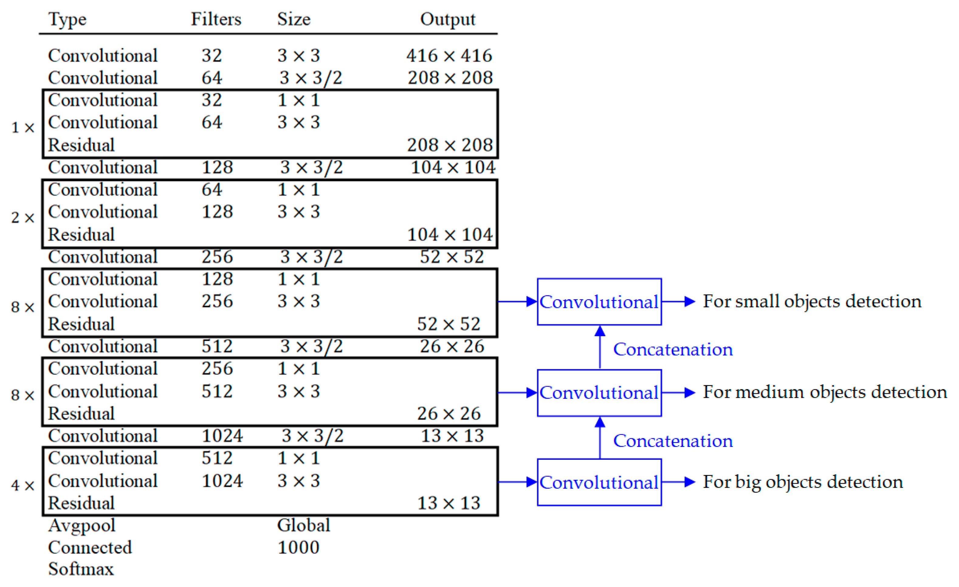
2.1. The CNN Algorithm

This study used the YOLO (You Only Look Once) algorithm, which was developed by Redmon and Farhadi [15,23,24] to be the core technology for mushroom image recognition and localization. The YOLOv3 is the third version and is based on the DarkNet-53 network structure. This algorithm achieves a better mean average precision (mAP) and shorter computing time. The MultiBox method was applied to YOLOv3 for object recognition [24]. The added Softmax layer with Box Regressor and Box Classifier transformed the MultiBox method into an object recognition method. This method directly predicts the category to which the object belongs. In YOLOv3, the training image is divided into N by N grid cells instead of ground truth box data. These grid cells are also used for box matching. The method involves making the target object image position fall into the appropriate grid cells. Each grid cell must be responsible for finding the exact location and category to which the object belongs. The details [23,24] of the YOLOv3 algorithm are discussed as follows.

2.1.1. Batch Normalization

The YOLOv3 algorithm enhances neural network convergence by the batch normalization of the training data [24]. It allows the features of each layer to be effectively passed to the next layer. This method reduces the reliance on other forms of regularization. This is because the neural network function is the distribution of the learning data. When the training data is different from the test (identification target) data distribution, the neural network’s ability to process general data is also reduced. Thus, the batch normalization of the training data is added to the convolutional layer and improves the accuracy of the network by about 2% in terms of the mAP. It also enables the data pattern to achieve the effect of regularization.

2.1.2. High Resolution Classifier

An image less than 256 × 256 is used for training and identification in most classifiers. This situation starts with the development of AlexNet. In YOLOv3, the image size is changed to more than 416 × 416. According to the experimental results, the recognition performance can be improved by using larger images [23,24].

2.1.3. Convolutional Neural Network with Anchor Boxes

Redmon et al [24] believed that spatial information is lost if the fully connected layer is used to detect the bounding box. This also leads to inaccurate localization. Therefore, the fully connected layer was discarded in the proposed approach. Anchor boxes were replaced to detect the bounding box. This idea is based on the practice of Faster R-CNN’s anchor box [20]. The sliding window sampling was applied to the feature map of convolution. Each detection point was predicted using nine sizes and proportions of Anchor Boxes. This method improves the recall rate [24].

2.1.4. Dimension Clusters of Anchor Box

In Faster R-CNN, the anchor box size is set manually. Redmon et al. proposed a new scheme to set the size. They obtained data from PASCAL Visual Object Classes (VOC) and Common Objects in Context (COCO) image databases, and used the K-means algorithm to determine the representative size of the anchor boxes. According to the literature [24], better detection results can be obtained by boxes which are obtained by K-means. There are nine boxes in YOLOv3: 10 × 13, 16 × 30, 33 × 23, 30 × 61, 62 × 45, 59 × 119, 116 × 90, 156 × 198, and 373 × 326.

2.1.5. Fine-Grained Features

The performance of the model for small-scale object detection can be improved by adding fine-grained features. The passthrough layer is added. This connects the feature map of the shallow layer to the deep one. The high-resolution and low-resolution feature maps are connected by the passthrough layer. The method of connecting is to stack adjacent features in different channels. This causes the size of feature map to change from 26 × 26 × 512 to 13 × 13 × 2048, and it is connected with the original deep feature map.

2.1.6. Multi-Scale Training

In order to make YOLOv3 robust to different size image recognition, an unfixed size of the input image is used in the training. The new image size is selected after every 10 batches of training. The down sampling parameter is set to 32 for the network. Multiples of 32 are used for the multi-scale training. The smallest image size is 320 × 320, and the largest is 608 × 608.

2.1.7. Training

The leaky and linear activation functions are used in the network. The leaky activation function is used in the convolutional layer and the linear activation function is used in the shortcut layer. The activation functions are shown as follows [8]:
Leaky   activation   function ,   ϕ ( x ) = { x , if   x > 0 0.1 x , otherwise
Linear   activation   function ,   ϕ ( x ) = x
In order to obtain the best prediction results and detect the position of the object in the image, the MSE (mean squared error) is designed for the loss function in YOLO. The loss function includes the calculating the errors of the bounding boxes coordinate regression, source prediction, and class score prediction. The loss function is shown in Equation (3) [15]. We use i j o b j to denote the jth bounding box of the ith grid to calculate the given object.
Loss   Function   =   λ c o o r d i = 0 S 2 j = 0 B i j o b j [ ( x i x ^ i ) 2 + ( y i y ^ i ) 2 ] + λ c o o r d i = 0 S 2 j = 0 B i j o b j [ ( w i w ^ i ) 2 + ( h i h ^ i ) 2 ] + i = 0 S 2 j = 0 B i j o b j ( C i C ^ i ) 2 + λ n o o b j i = 0 S 2 j = 0 B i j n o o b j ( C i C ^ i ) 2 + i = 0 S 2 i o b j c c l a s s e s ( p i ( c ) p ^ i ( c ) ) 2
where the first and second terms are the bounding boxes coordinate regression of the position and the size error in the bounding box; the third and fourth terms are the calculations of the bounding box source prediction; and the fifth term is the calculation of the class score prediction. The remaining parameters are explained as follows:
  • λ c o o r d , λ n o o b j are constants, ( λ c o o r d = 5 , λ n o o b j = 0.5 );
  • x i , y i are the center coordinates of the ith anchor box;
  • x ^ i , y ^ i are the center coordinates of the ith known ground truth box;
  • w i , h i are the width and height of the ith anchor box;
  • w ^ i , h ^ i are the width and height of the ith ground truth box;
  • C i is the confidence score of the ith objectness;
  • C ^ i is the objectness of the ith ground truth box;
  • p i ( c ) is the classification loss of the ith object; and
  • p ^ i ( c ) is the classification loss of the ith ground truth box.

2.1.8. Detection Purpose Training
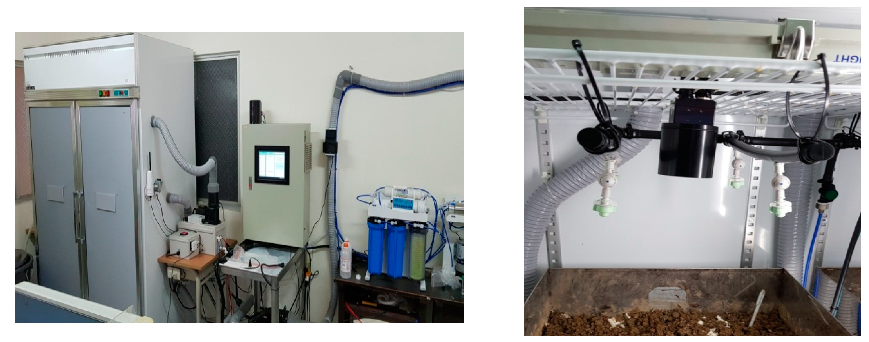
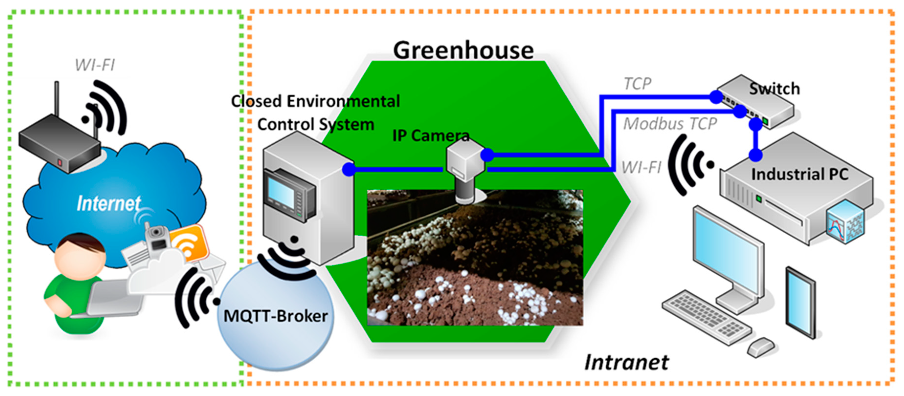
In order to change the classification network into a detection network, the last convolutional layer was removed and three 3 × 3 (1024 feature generator) convolutional layers were added in YOLOv3. A 1 × 1 convolutional layer followed in every convolutional layer. The output dimension was the quantity required to detect. The continuous 3 × 3 and 1 × 1 convolutional layers were formed and used in the YOLOv3 network. The network structure is called DarkNet-53 and is shown in Figure 1 [24]. DarkNet-53 refers to the method of residual network. DarkNet-53 is a 53-layer feature extracting deep neural network which includes 52 convolutional layers and one connected layer. In addition, each layer is processed by batch normalization and leaky activation. For a 416 × 416 input image, it is a grid of 13 × 13 cells. Each grid cell must be responsible for finding the exact location and category to which the object belongs. DarkNet-53 uses three scales to detect big objects, medium objects, and small objects. The relative three resultant feature map sizes are 13 × 13, 26 × 26, and 52 × 52.

2.2. System Design

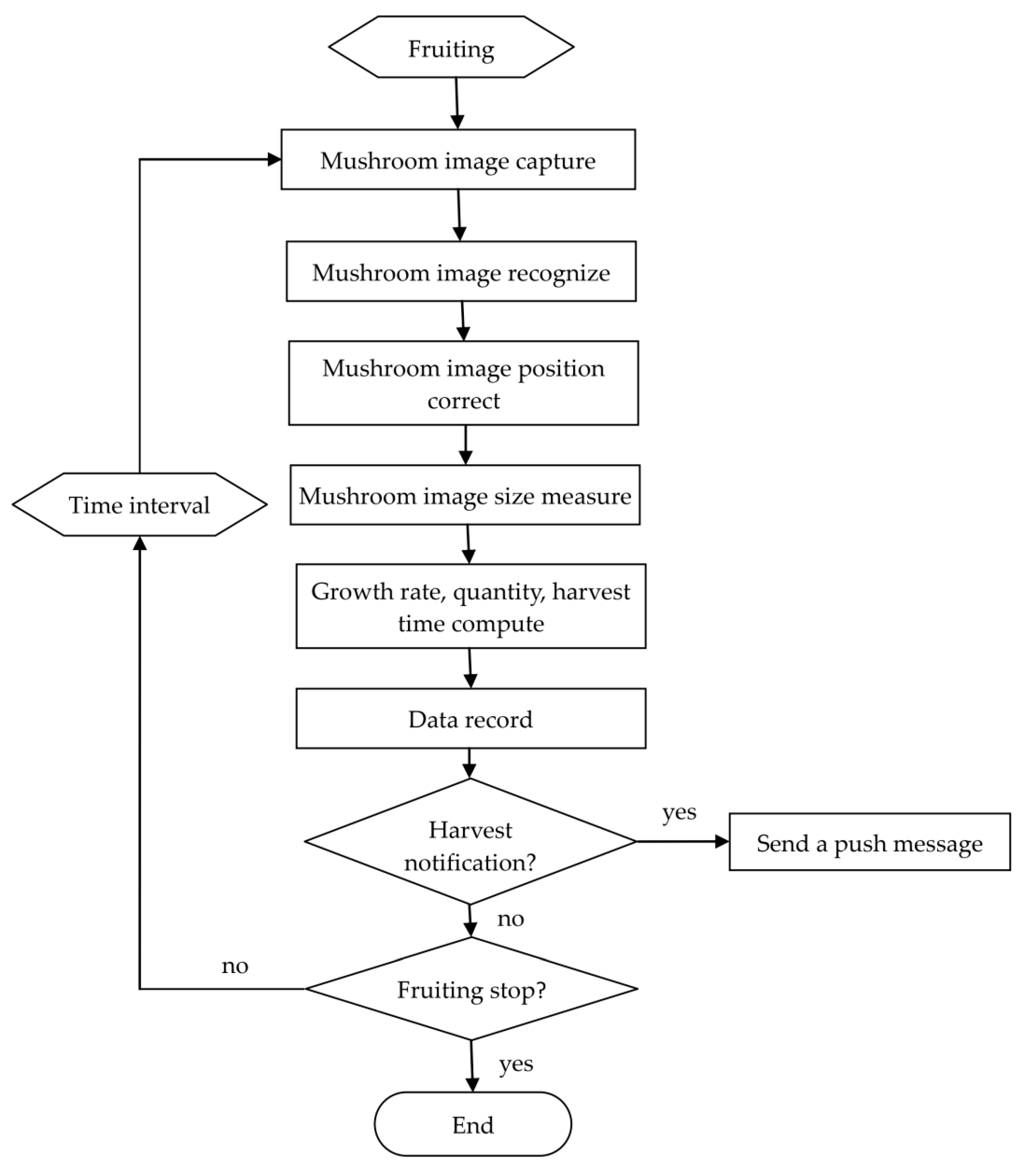
2.2.1. System Overview

We built a small mushroom greenhouse for experimentation and system verification. The built greenhouse is shown in Figure 2. The greenhouse was built and modified by a general closed refrigerator. Many kinds of sensors were installed in the greenhouse to measure the temperature, humidity, and carbon dioxide level. The temperature and humidity of the soil were also measured in the greenhouse. The designed watering module was used to automatically maintain the moisture in the soil. We also designed a microclimate regulator to control the temperature, humidity, and carbon dioxide level. We designed our own fuzzy controller to control the microclimate by closed loop equipment. The communication structure of our system is shown in Figure 3. The TCP/IP protocol was used for communication and the IP network camera was used for capturing the mushroom images. The software, YOLOv3 algorithm, and image processing algorithm were developed using C++ language. An industrial computer was used for calculations. We used CPU to execute the YOLOv3 algorithm. The MQTT Broker was used for message broadcasting [25]. The system employed included the Publisher, which broadcast the message to the Subscriber (mobile device) according to the image analysis results.
The calculation flow chart is shown in Figure 4. The growth measurement of mushrooms was mainly conducted in the mushrooming stage. After the spawn running stage, the mushrooming stage started after two weeks of covering soil treatment and the mushroom image measurement function also began at this time. The measuring frequency was once in one hour and the measurement process is shown in Figure 4. Since the growth environment of mushrooms requires a low light state, the light source was often turned off. The light source was thus turned on when the system captured images, for a duration of less than one minute. The total time for the following image processing, including the data being recorded in the database, took less than 10 min. After the mushroom images were captured, the YOLOv3 algorithm was executed to recognize and localize the mushrooms. Every mushroom position was marked and corrected by the last localization result. Next, the size, amount, growth rate, and estimated harvest time were calculated. Every data point for every mushroom was recorded in the database and used to calculate the growth curve and growth rate of the mushrooms. We also estimated the size and the number of harvested mushrooms. All the data were analyzed and the results were broadcasted to the user.

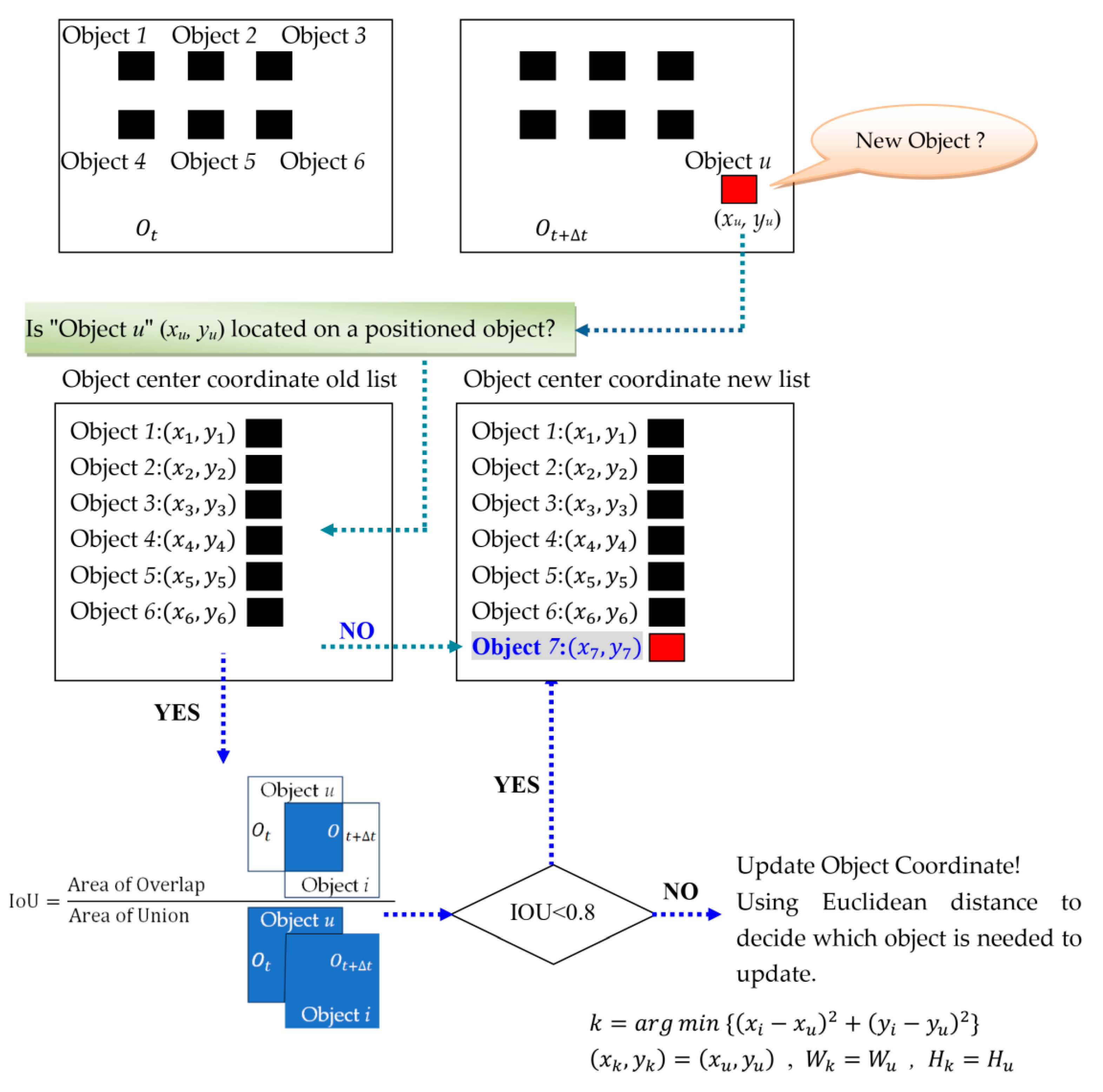
2.2.2. Positioning Correction Method

Uneven illumination and shadowing have a serious impact on image measurement in practical applications. It is also easy to make image recognition errors. This study addresses the above problems. For example, a result of the mushroom localization and recognition is shown in Figure 5 with different capturing times. The first result is shown in Figure 5a, where the time is denoted as O t . After a specific interval, the time is denoted as O t + Δ t ( Δ t is set as one hour), at which point we captured another image and the recognition result is shown in Figure 5b. We can see that mushrooms A and B can be detected in Figure 5a but are missed in Figure 5b. The recognition results with images captured at times O t + 2 Δ t and O t + 13 Δ t are shown in Figure 5c,d, respectively. We can see that a few mushrooms cannot be located using the first identification process, but they are detected in the other process. In order to solve this problem, a positioning correction algorithm was designed in this paper. The algorithm flowchart is shown in Figure 6.
The positioning correction algorithm is based on the first results of the mushroom localization. Taking Figure 6 as an example, the time of the first positioning is O t , and six objects are recognized (Object 1, Object 2, …, Object 6). The coordinates (xi, yi), width ( W i ), and height ( H i ) of each object are recorded. The next time of positioning is O t + Δ t , and the results are based on the previous positioning results. If the center coordinates of a recognized object (Object u) is not located on a positioned object, the recognized object is new one. When the coordinates of “Object u” are located on a positioned object, the Intersection over Union (IoU) is executed to calculate the proportion of overlapping area. In order to reduce unnecessary calculations, we find “Object k”, which is closest to “Object u” to perform IoU. “Object u” is set to be a new object if IoU is less than 0.8; otherwise it is set to “Object k”. The minimum distance object estimation formula is as follows:
k = a r g   m i n { ( x i x u ) 2 + ( y i y u ) 2 } .
The new object judgment formula is as follows:
Object   u = { u = k ,   ( x k ,   y k ) = ( x u ,   y u )   , W k = W u   ,   H k = H u if   IOU 0.8 u = new   object   if   IOU < 0.8
After executing the positioning correction algorithm, the result of the neural network positioning error can be corrected, and the positioning accuracy of the mushroom can be improved.

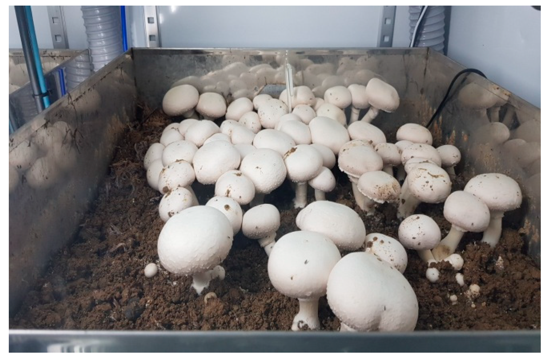
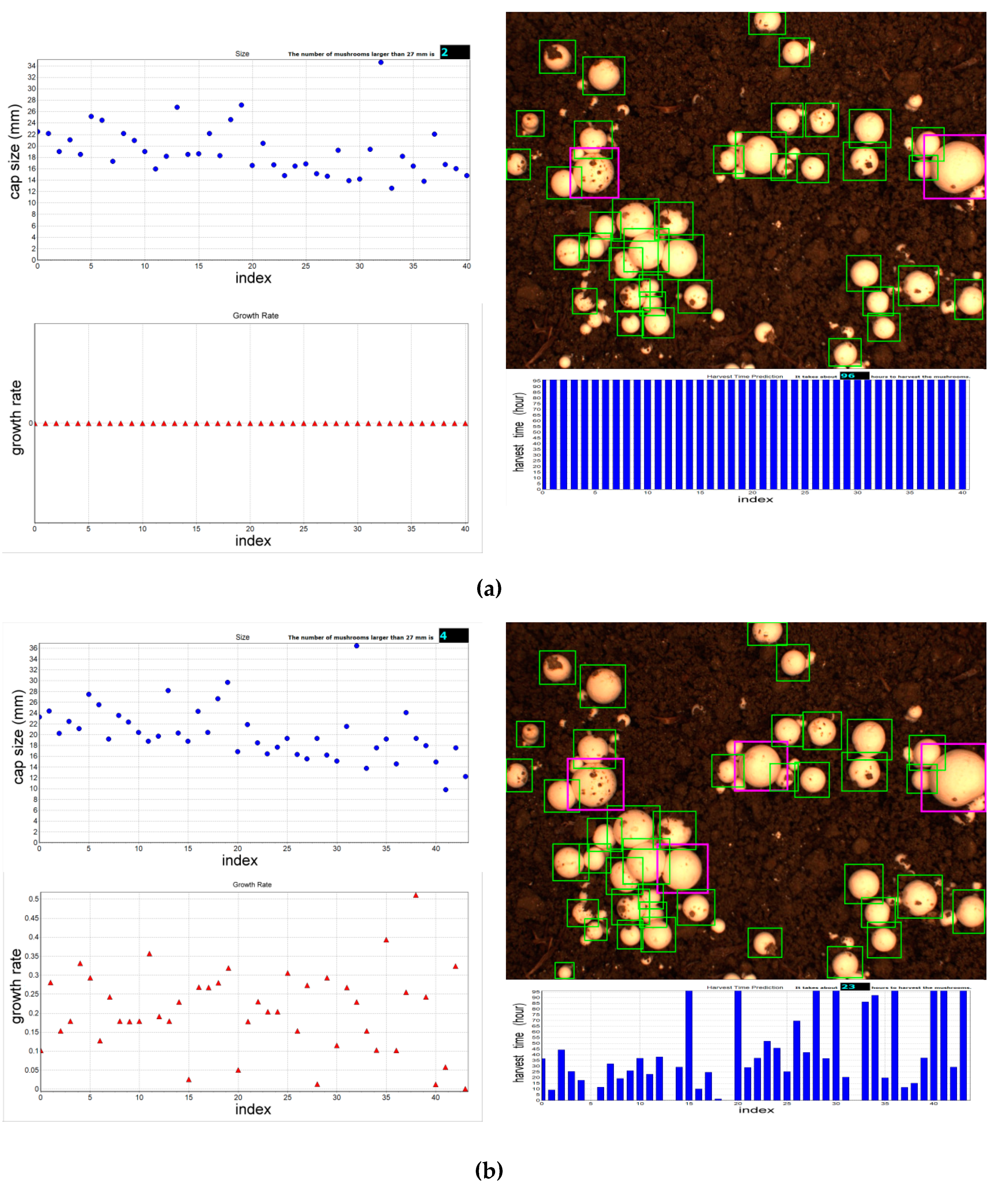
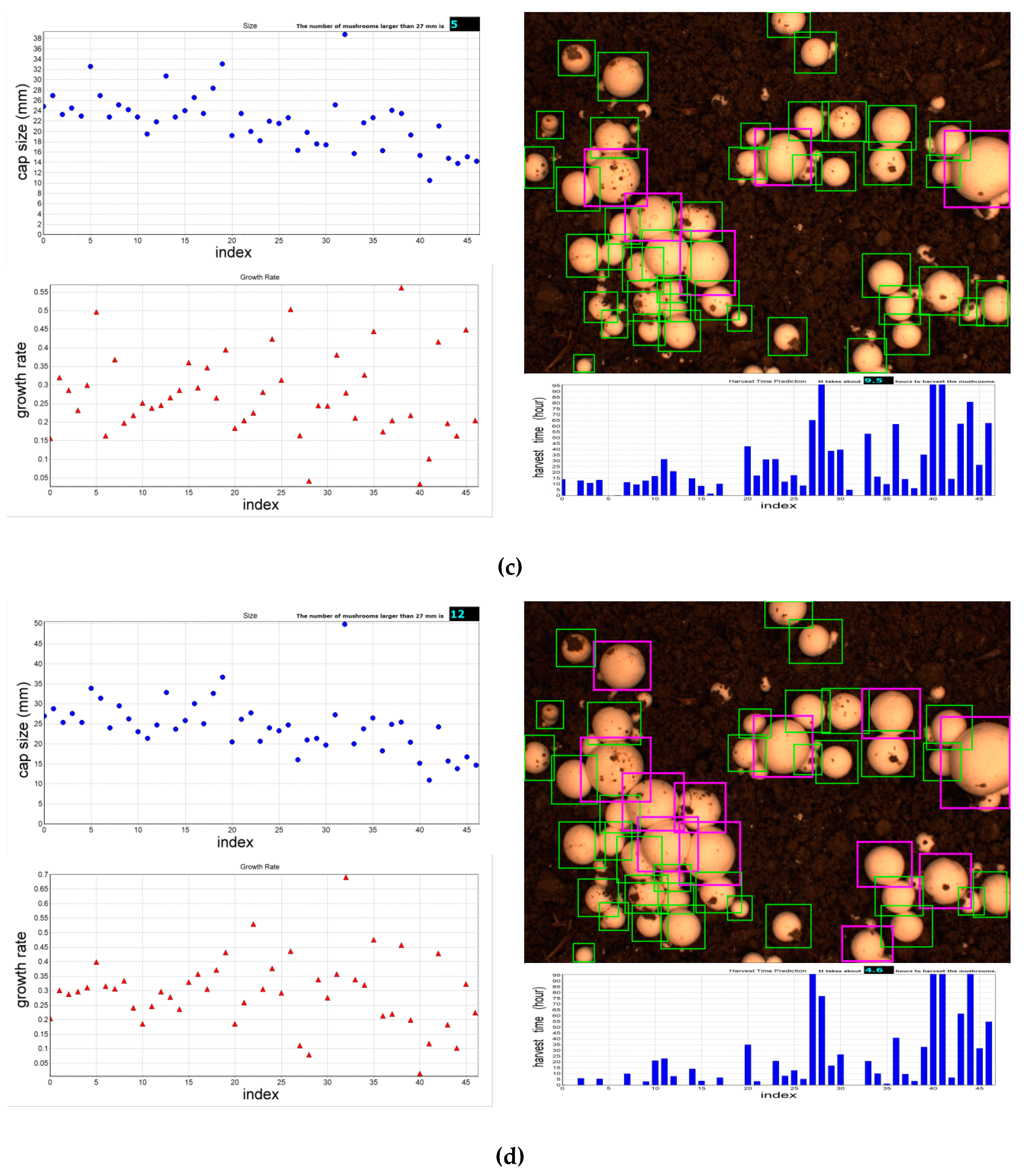
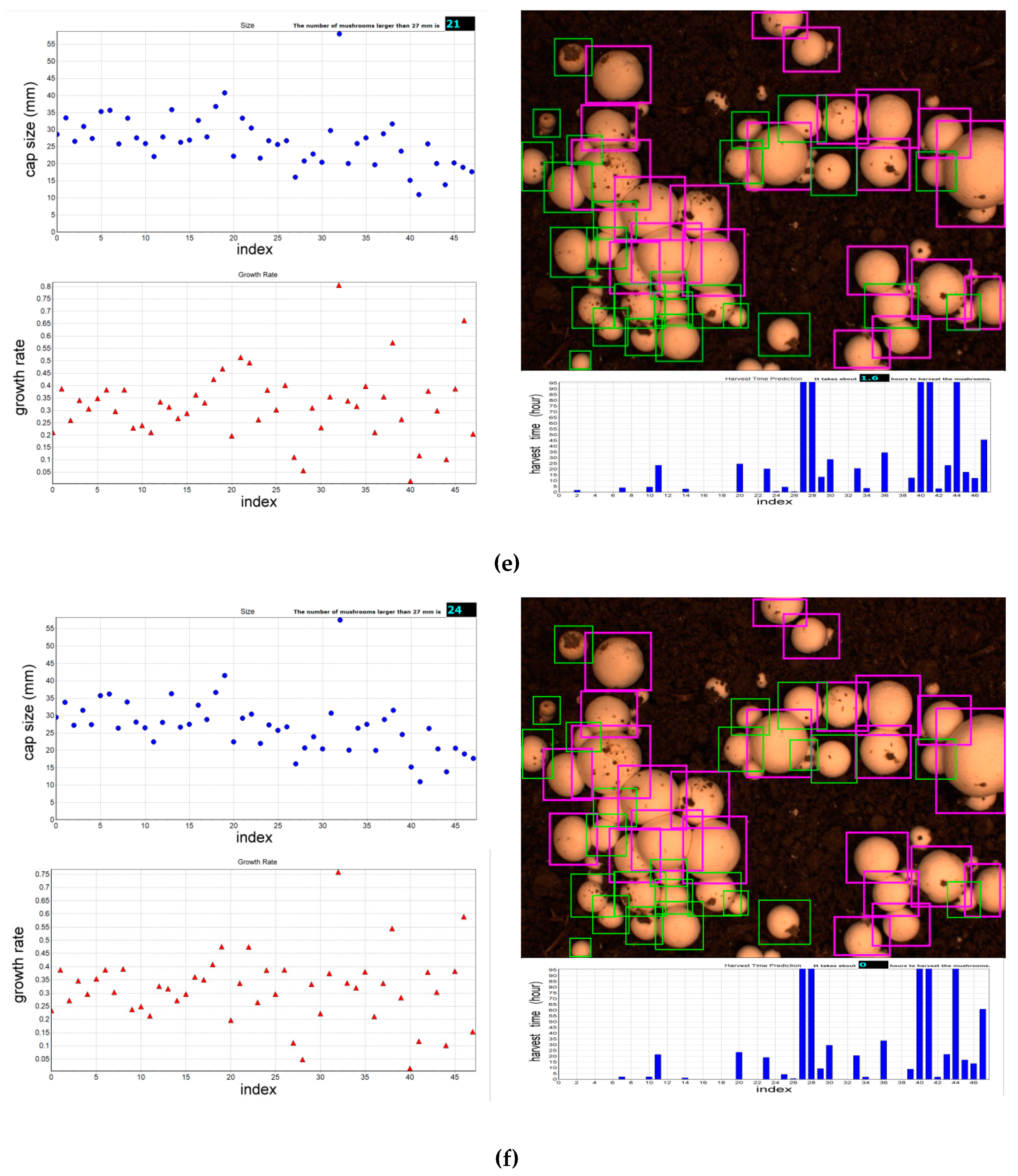
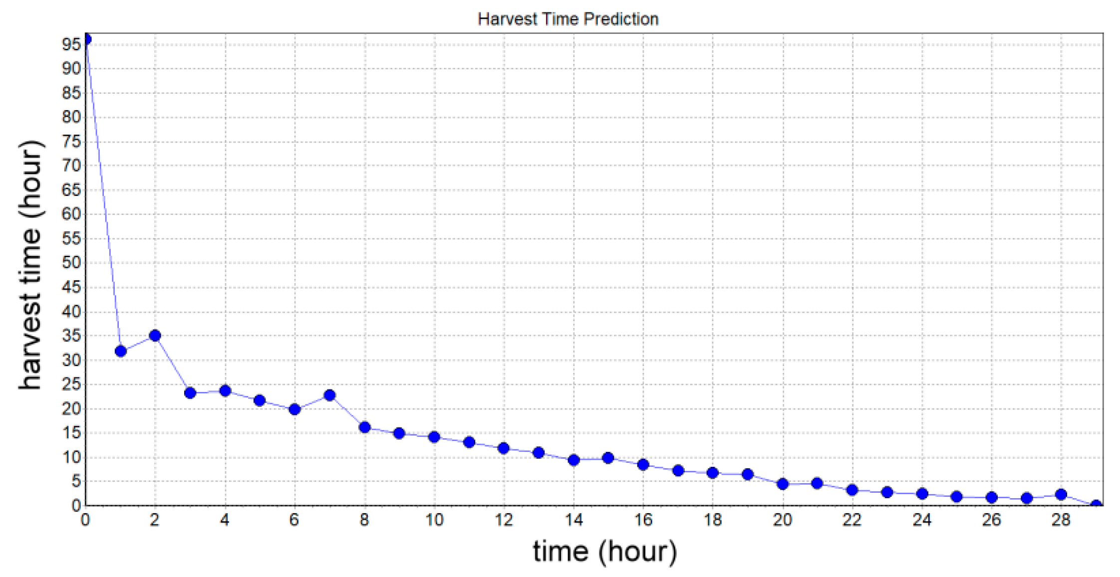
2.2.3. Estimation of Cap Size, Growth Rate, Amount, and Harvest Time

In this study, the number of mushrooms in the unit area, the size of the mushroom cap, and the growth rate are the features used to evaluate the growth status of the mushrooms. The number of mushrooms can be calculated after obtaining the positioning results from the image processing. The size of the bounding box is set to be the size of the mushroom cap. Most of the bounding box shapes are close to squares, although some bounding boxes that fall on the edge of an image are rectangles. The mushroom size is denoted as S (pixels) and is computed using the following equation:
S = { W if   W > 1.5 H H if   H > 1.5 W ( W + H ) / 2 Others
After obtaining the mushroom size, S , it is multiplied by the resolution of the image, R (mm/pixel), to estimate the actual size of the mushrooms, S ¯ .
S ¯ = S × R
The growth rate, G , is calculated by the dimensional change of the mushroom in a time period. It is also compared to the first measured size. The growth rate, G (mm/hr), is denoted as:
G = S ¯ n S ¯ 1 M
where S ¯ 1 is the first measurement result, S ¯ n is the n th measurement result, and M is the time period from S ¯ 1 to S ¯ n . The harvest time, T , is estimated by:
T = S ˜ S ¯ t G
where S ˜ is the expected harvest size of the mushrooms.

2.2.4. Human Machine Interface

The Embarcadero C++ Builder was used to develop the proposed system. The Windows SDK was also used to build the multi-thread image detection system. The interface has the advantage of easy operation, as shown in Figure 7. The user only needs to set the image measurement period (Model I/II/III) and the expected harvest size of the mushrooms. The rest are automatic executed by the designed system. The MQTT is used for message broadcasting. The measurement system is set as the Publisher, the MQTT server is set locally to be the Broker, and the Subscriber is the corresponding app on a mobile phone.

3. Results

The experimental results in this paper were obtained from the built greenhouse (shown in Figure 2). The light source of the camera was a fluorescent light. The remote controller of the light source was an LC-103 relay that produced by ICP-DAS CO., LTD. The Modbus RTU was used to transmit the on and off commands to the light source. The images were captured within the set time period (1 h for the Model I). The IP network camera used was an SVS-VISTEK (ECO445CVGE67) IP67. The image was transmitted by TCP protocol with a size of 1296 × 964. The image was taken from a distance of about 22 cm. The algorithm was performed on an Axiomtek EBOX635-881-FL I5 2.7 GHz industrial computer. The results are discussed as follows.

3.1. Sample Training

We collected 500 mushroom images as the training sample and labeled them using a tool called LabelImg [26]. We performed 10,000 iterative iterations and used the weights obtained after the sample training to identify the mushrooms. An image processing card with Nvidia Quadro P4000 GPU was used to train the sample. We also set the required parameters for YOLOv3. The setting and functions are explained as follows.
  • Number of training images (batch = 64). This parameter sets the number of images for each training sample (64 in this paper). This parameter must be adjusted according to the memory size of the image processing card.
  • Number of segment training (subdivisions = 16). In order to match the Nvidia CUDA library (executing GPU), this parameter allows the training image to be segmented. After one by one execution, the iterative process is completed again.
  • The input image was set as 416 by 416 with 24-bit color (channels = 3). All the original images were resized to match the input image.
  • Regional comparison rate (momentum = 0.9). It is not easy to find the best value if this parameter is set larger than 1.
  • Weight attenuation ratio (decay = 0.0005). This parameter is used to reduce the possibility of overfitting.
  • Diversified parameters (angle = 0, saturation = 1.5, exposure = 1.5, hue = 0.1). These are used to adjust the rotation, saturation, exposure, and hue of the image. This is to enhance the diversification of the sample and improve the practical recognition effect of the image.
  • Network learning rate (learning rate = 0.001). This parameter is used to determine the speed of the weight adjustment. A larger value indicates a smaller number of calculations, but divergence may occur. As the number becomes smaller, the convergence speed becomes slower, and it is easy to find the result of local optimization.
  • The maximum number of iterations was 10,000 (max batches = 10,000).
  • Learning policies are Fixed, Step, Exp, Inv, Multistep, Poly, or Sigmoid. We used Step in the YOLOv3 algorithm.
  • The number of feature generation filters was 18 (filter = 18).
  • Number of object categories was 1 (classes = 1). The mushroom is the only object in this study.

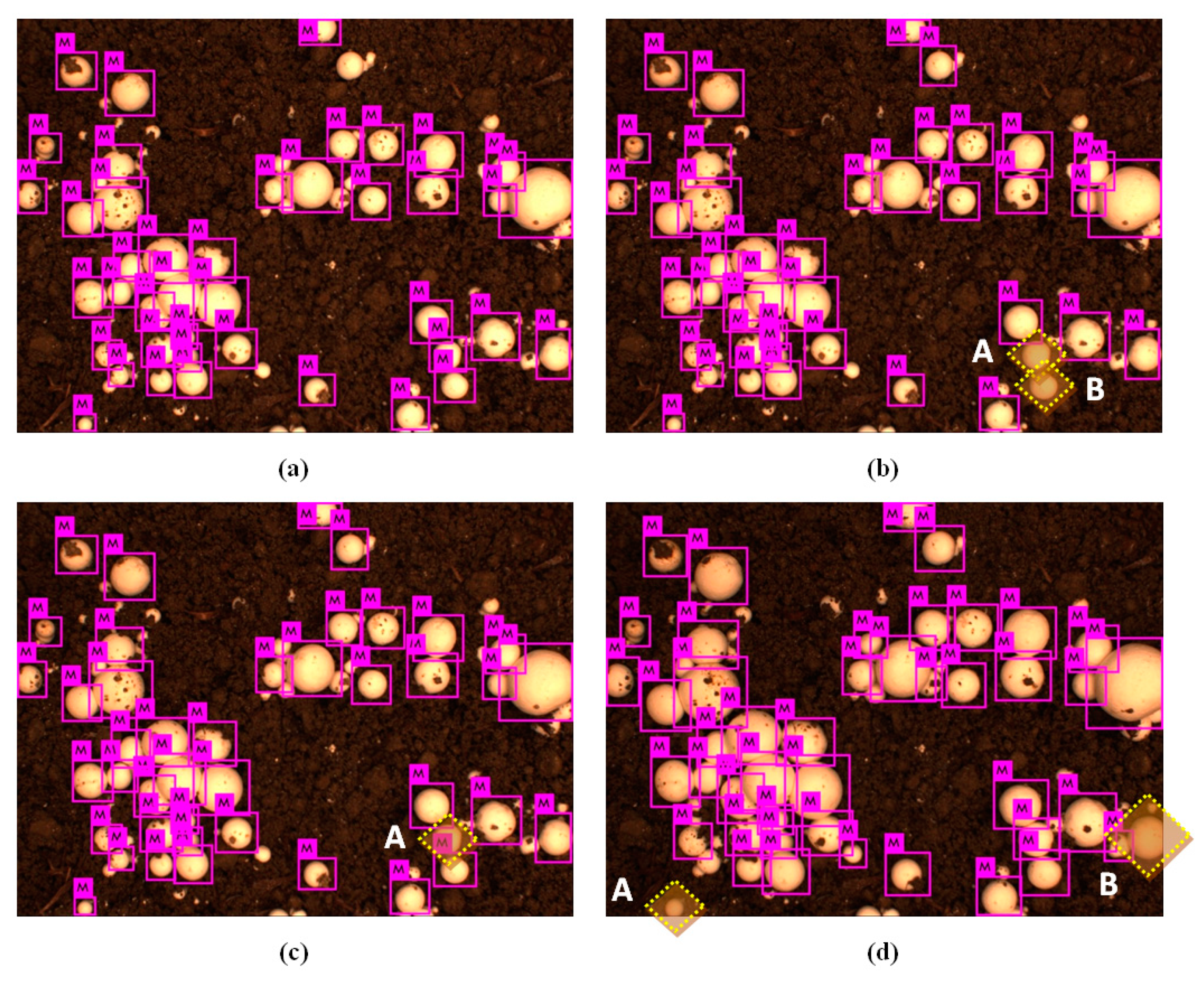
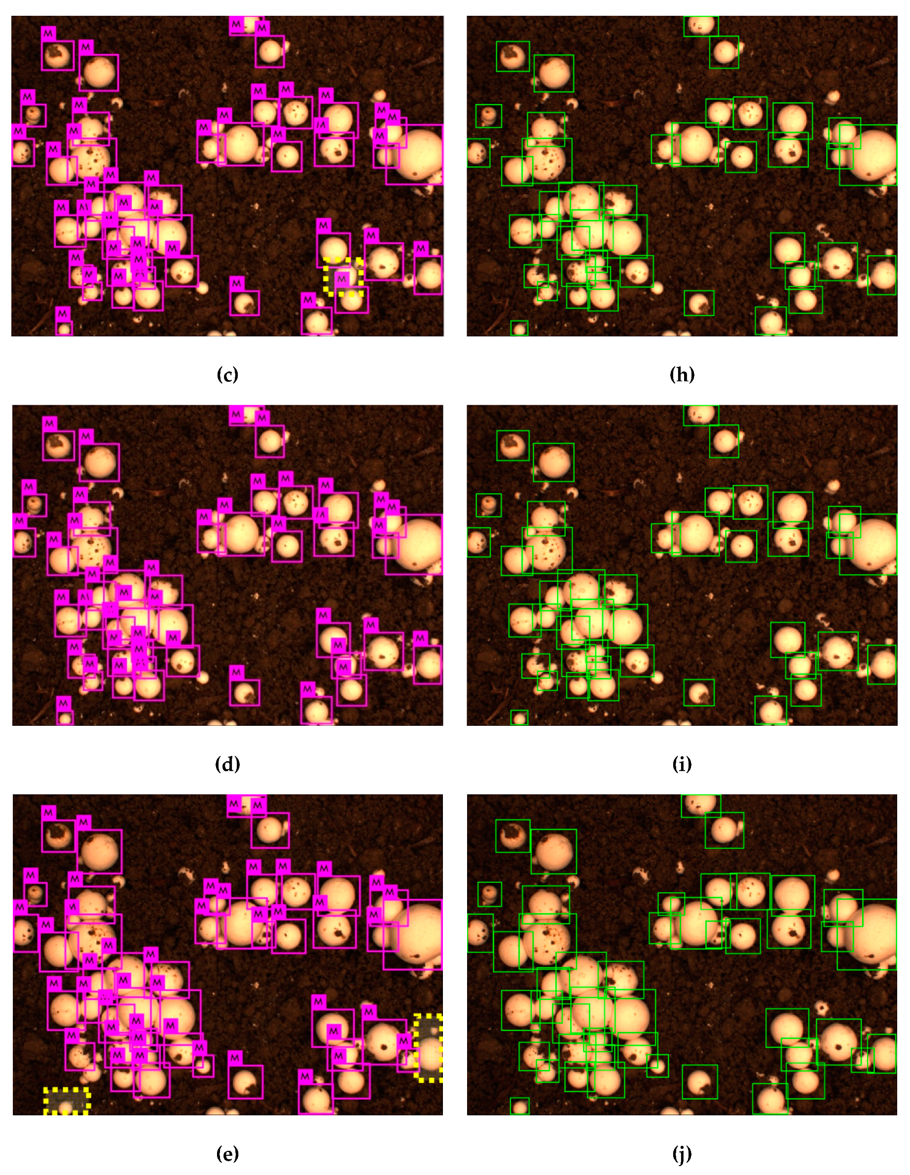
3.2. The Experiment of Mushroom Positioning Correction

The period of the positioning correction is one harvest cycle. A single planting procedure (fermentation, spawn running, soil covering, and mushrooming) includes three harvest cycles. When the mushroom grows to the target size and the number of mushrooms reaches a set value, the mushroom measurement system is stopped. Or, when the system reaches a set time, the measurement system is also stopped. A message is sent when the system is stopped and the system then waits for the next harvest cycle. The first captured mushroom image is set to be the initial position for each positioning correction. The experiment results are shown in Figure 8, where Figure 8a–e are the original positioning images and Figure 8f–h are the the positioning correction results. The difference in image positioning of each mushroom is framed by a yellow dotted line. We can see that the positioning correction is effective to make up the missing area.

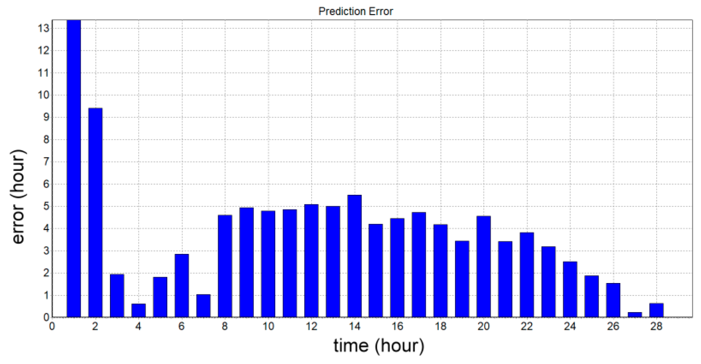
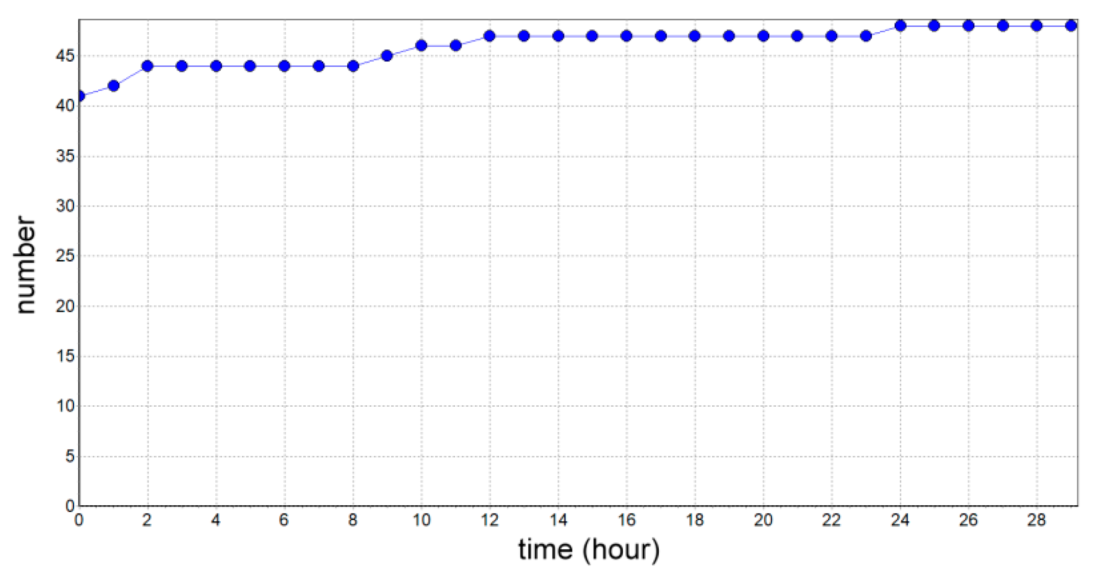
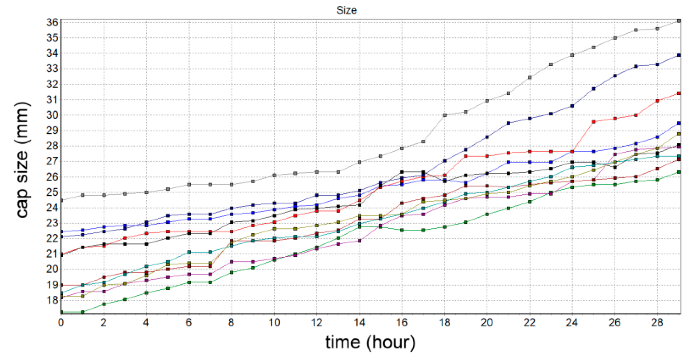
3.3. The Experiments of Cap Size, Growth Rate, Amount, and Harvest Time Estimation

In the designed system, the resolution of the mushroom image is 4.9 pixels/mm. The camera takes an image from a distance of about 22 cm. The captured image size is 1296 × 964 pixels. The growth estimation is started at the first image analysis. The size change of each mushroom detected is used to calculate the growth rate. The system calculates the growth rate of each mushroom one by one and accumulates the number of located mushrooms. We set the mushroom size to 27 mm. The experiment results of the measurement of mushrooms at six time points are shown in Figure 9. In order to clearly observe the growth of mushrooms, the data only shows the results after the diameter of the mushroom exceeds 10 mm. The left side of Figure 9 shows the cap size and growth rate. The right side of Figure 9 shows the positioning results and estimated harvest time. The system estimates the harvest time based on the set harvest size. The estimated harvest time is calculated by the average harvest time of 50% of the largest mushrooms. The system also broadcasts the message by MQTT as shown in Figure 10.
In the experiment depicted in Figure 9, the measurement is automatically executed every hour. Figure 9a is the start of the measurement and the growth rate was 0 for each mushroom at that time. Forty-one mushrooms were detected in the first positioning. The detected mushrooms were denoted as No. 0–No. 40. Two mushrooms were detected as larger than the expect harvested size (we marked them with purple squares). They were No. 19 (27.2 mm) and No. 32 (34.6 mm). The initial harvest time was 96 h. Figure 9b shows the measurement results after 7 h. There were 44 mushrooms detected. Four mushrooms were newly detected, where No. 43 was the newest detected mushroom at the 7th hour. Its growth rate was 0 and its harvest time was estimated as 23 h. The results after 14 h are shown in Figure 9c. The number of detected mushrooms was 47. There were three new detected mushrooms at this time and five mushrooms had reached the designated harvest size. The estimated harvest time for the top 50% mushrooms was 9.5 h. After 21 h, the result is shown in Figure 9d. The number of detected mushrooms was 47. There was no new detected mushroom but 12 mushrooms reached the harvest size. The estimated harvest time was 4.6 h. Figure 9e shows the results at 28 h. There were 21 mushrooms that satisfied the harvest size out of 48 detected mushrooms, and the estimated harvest time was 1.6 h. At 29 h, the results are shown in Figure 9f. There were 24 mushrooms bigger than the designated harvest size out of 48 detected mushrooms. At this time, the goal of 50% of the mushrooms being ready for harvesting was achieved and the estimated harvest time was 0 h. Please denote that there was one mushroom with a growth rate of 0.
We collect all estimated harvest times in the 29 h and show the results in Figure 11. We also used the known harvest time to compute the estimated error. The errors of each time are shown in Figure 12 and the average error was 3.7 h. The numbers of detected mushrooms at each measurement time are shown in Figure 13. We can see that the bigger mushrooms were easier to identify by the YOLOv3 algorithm. This does not affect the performance of the system because the small mushrooms are not considered harvesting objects. We also randomly selected 10 mushrooms to record the growth size and the results of these are shown in Figure 14. The experiment data can be a reference for the conditions related to plant mushrooms.

4. Conclusions

A smart mushroom measurement system using image processing technology is proposed in this paper. The system automatically measures and records the size of the mushroom cap and the growth rate during the fruiting body formation. The harvest time can be estimated by the obtained data. The obtained data can not only be the parameters of the greenhouse, but also the important indicators of production management. This system has the potential to become an expert system for smart environment control. The proposed system is based on the convolutional neural network of deep learning to localize mushrooms in the obtained images. A positioning correction method is also proposed to modify the positioning results. The experiments show that the proposed system has good performance in terms of the image measurement of mushrooms. This system can be applied to the other mushrooms with a similar geometry. In the future, the proposed system may be combined with greenhouse control systems to optimize the best conditions for mushroom growth. The collected data and proposed algorithm may also enable the development of artificial intelligence for agricultural systems.

Author Contributions

C.-P.L. and J.-J.L. designed the algorithm and experiments and wrote the article. C.-P.L. completed the software development and experimental verification. T.-C.W. and T.-F.H. conducted experiments and performed data collection.

Acknowledgments

This work was supported in part by the Ministry of Science and Technology, Taiwan, R.O.C., under grant MOST 106-2221-E-276 -001. The authors thank the Pingtung “Ching Tuan Mushroom Farm”. Mr. Lin provided all the materials and experience of mushroom cultivation for this research.

Conflicts of Interest

The authors declare no conflict of interest.

References

  1. Zhou, J.-H.; Zuo, Y.-M. Application of Computer Control System in the Greenhouse Environmental Management. In Proceedings of the 2009 International Conference on Future BioMedical Information Engineering, Sanya, China, 13–14 December 2009; pp. 204–205. [Google Scholar]
  2. Zhang, C.-F.; Chen, Y.-H. Applications of DMC-PID Algorithm in the Measurement and Control System for the Greenhouse Environmental Factors. In Proceedings of the 2011 Chinese Control and Decision Conference, Nanchang, China, 23–25 May 2011; pp. 483–485. [Google Scholar]
  3. Idris, I.; Sani, M.I. Monitoring and control of aeroponic growing system for potato production. In Proceedings of the 2012 IEEE Conference on Control, Systems & Industrial Informatics, Bandung, Indonesia, 23–26 September 2012; pp. 120–125. [Google Scholar]
  4. Liu, Q.; Jin, D.; Shen, J.; Fu, Z.; Linge, N. A WSN-Based prediction model of microclimate in a greenhouse using extreme learning approaches. In Proceedings of the 2016 18th International Conference on Advanced Communication Technology, PyeongChang, South Korea, 31 January–3 February 2016; pp. 730–735. [Google Scholar]
  5. Wu, W.-H.; Zhou, L.; Chen, J.; Qiu, Z.; He, Y. GainTKW: A measurement system of thousand kernel weight based on the android platform. Agronomy 2018, 8, 178. [Google Scholar] [CrossRef]
  6. Gong, L.; Lin, K.; Wang, T.; Liu, C.-L.; Yuan, Z.; Zhang, D.-B.; Hong, J. Image-Based on-panicle rice [Oryza sativa L.] grain counting with a prior edge wavelet correction model. Agronomy 2018, 8, 91. [Google Scholar] [CrossRef]
  7. Zhang, C.-Y.; Si, Y.-S.; Lamkey, J.; Boydston, R.A.; Garland-Campbell, K.A.; Sankaran, S. High-throughput phenotyping of seed/seedling evaluation using digital image analysis. Agronomy 2018, 8, 63. [Google Scholar] [CrossRef]
  8. Goodfellow, I.; Bengio, Y.; Courville, A. Deep Learning; MIT Press: London, UK, 2016; ISBN 0262035618. [Google Scholar]
  9. Krizhevsky, A.; Sutskever, I.; Hinton, G.E. Imagenet classification with deep convolutional neural networks. Adv. Neural Inf. Proc. Syst. 2012, 1, 1097–1105. [Google Scholar] [CrossRef]
  10. Girshick, R.; Donahue, J.; Darrell, T.; Malik, J. Rich Feature Hierarchies for Accurate Object Detection and Semantic Segmentation. In Proceedings of the 2014 IEEE Conference on Computer Vision and Pattern Recognition, Columbus, OH, USA, 23–28 June 2014. [Google Scholar]
  11. Sermanet, P.; Eigen, D.; Zhang, X.; Mathieu, M.; Fergus, R.; LeCun, Y. Overfeat: Integrated recognition, localization and detection using convolutional networks. In Proceedings of the 2013, OverFeat: Integrated Recognition, Localization and Detection Using Convolutional Networks, International Conference on Learning Representations, Banff, AB, Canada, 14–16 April 2013. [Google Scholar]
  12. Zeiler, M.D.; Fergus, R. Visualizing and understanding convolutional networks. In Computer Vision—ECCV 2014. Lecture Notes in Computer Science; Springer: Cham, Switzerland, 2014; Volume 8689, pp. 818–833. [Google Scholar] [CrossRef]
  13. He, K.; Zhang, X.; Ren, S.; Sun, J. 2015 Spatial pyramid pooling in deep convolutional networks for visual recognition. IEEE Trans. Pattern Anal. Mach. Intell. 2015, 37, 1904–1916. [Google Scholar] [CrossRef] [PubMed]
  14. Girshick, R. Fast R-CNN. In Proceedings of the 2015 IEEE International Conference on Computer Vision, Santiago, Chile, 11–18 December 2015; pp. 1440–1448. [Google Scholar]
  15. Redmon, J.; Divvala, S.; Girshick, R.; Farhadi, A. You Only Look Once: Unified, Real-Time Object Detection. In Proceedings of the 2016 IEEE Conference on Computer Vision and Pattern Recognition, Las Vegas, NV, USA, 26 June–1 July 2016; pp. 779–788. [Google Scholar]
  16. Simonyan, K.; Zisserman, A. Very Deep Convolutional Networks for Large-Scale Image Recognition. In Proceedings of the 2015 International Conference on Learning Representations, San Diego, CA, USA, 7–9 May 2015; pp. 1–14. [Google Scholar]
  17. Szegedy, C.; Liu, W.; Jia, Y.; Sermanet, P.; Reed, S.; Anguelov, D.; Erhan, D.; Vanhoucke, V.; Rabinovich, A. Going Deeper with Convolutions. In Proceedings of the 2015 IEEE Conference on Computer Vision and Pattern Recognition, Boston, MA, USA, 7–12 Jun 2015; pp. 1–9. [Google Scholar]
  18. Szegedy, C.; Reed, S.; Erhan, D.; Anguelov, D. Scalable, High-Quality Object Detection. arXiv Preprint, 2015; arXiv:1412.1441. [Google Scholar]
  19. He, K.; Zhang, X.; Ren, S.; Sun, J. Deep Residual Learning for Image Recognition. In Proceedings of the 2016 IEEE Conference on Computer Vision and Pattern Recognition, Las Vegas, NV, USA, 26 June–1 July 2016; pp. 770–778. [Google Scholar]
  20. Ren, S.; He, K.; Girshick, R.; Sun, J. Faster R-CNN: Towards real-time object detection with region proposal networks. IEEE Trans. Pattern Anal. Mach. Intell. 2017, 39, 1137–1149. [Google Scholar] [CrossRef] [PubMed]
  21. Liu, W.; Anguelov, D.; Erhan, D.; Szegedy, C.; Reed, S.; Fu, C.-Y.; Berg, A.C. SSD: Single shot multibox detector. In Computer Vision—ECCV 2016. Lecture Notes in Computer Science; Springer: Cham, Switzerland, 2016; Volume 9905, pp. 21–37. [Google Scholar] [CrossRef]
  22. He, K.; Gkioxari, G.; Dollár, P.; Girshick, R. Mask R-CNN. In Proceedings of the 2017 IEEE International Conference on Computer Vision, Venice, Italy, 22–29 October 2017; pp. 2980–2988. [Google Scholar]
  23. Redmon, J.; Farhadi, A. YOLO9000: Better, Faster, Stronger. In Proceedings of the 2017 IEEE Conference on Computer Vision and Pattern Recognition (CVPR), Honolulu, HI, USA, 21–26 July 2017; pp. 6517–6525. [Google Scholar]
  24. Redmon, J.; Farhadi, A. YOLOv3: An Incremental Improvement (Tech Report). 2018. Available online: https://pjreddie.com/media/files/papers/YOLOv3. pdf (accessed on 1 November 2018).
  25. MQTT. Available online: http://mqtt.org (accessed on 15 November 2018).
  26. LabelImg. Available online: https://github.com/tzutalin/labelImg (accessed on 3 November 2018).
Figure 1. The structure of the DarkNet-53 network.
Agronomy 09 00032 g001
Figure 2. The small greenhouse for the experimental crops planted.
Agronomy 09 00032 g002aAgronomy 09 00032 g002b
Figure 3. The communication structure of the mushroom measurement system.
Agronomy 09 00032 g003
Figure 4. The flowchart of the measurement system.
Agronomy 09 00032 g004
Figure 5. Positioning results of mushrooms at different times: (a) O t , (b) O t + Δ t , (c) O t + 2 Δ t , and (d) O t + 13 Δ t .
Agronomy 09 00032 g005
Figure 6. The flowchart of the positioning correction.
Agronomy 09 00032 g006
Figure 7. The human machine interface of the mushroom measurement system.
Agronomy 09 00032 g007
Figure 8. The experiments of positioning correction. The original positioning image at (a) 0 h, (b) 1 h, (c) 2 h, (d) 3 h, and (e) 13 h. (f) The initial positioning, (g) the first positioning correction, (h) the second positioning correction, (i) the third positioning correction, and (j) the 13th positioning correction.
Agronomy 09 00032 g008aAgronomy 09 00032 g008b
Figure 9. The measurement results at (a) the first time, (b) 7 h (7th), (c) 14 h (14th), (d) 21 h (21th), (e) 28 h (28th), and (f) 29 h (29th).
Agronomy 09 00032 g009aAgronomy 09 00032 g009bAgronomy 09 00032 g009c
Figure 10. The broadcast message indicating the estimated harvest time.
Agronomy 09 00032 g010
Figure 11. The estimated harvest time in 29 h.
Agronomy 09 00032 g011
Figure 12. The errors of the estimated harvest time.
Agronomy 09 00032 g012
Figure 13. The number of detected mushrooms in 29 h.
Agronomy 09 00032 g013
Figure 14. The sizes of 10 randomly selected mushrooms.
Agronomy 09 00032 g014

