Quantifying Socioeconomic Potential Losses Under Water Scarcity Using the WIOLP Model

Abstract

The increasing frequency and severity of extreme droughts caused by climate change has emerged as a key risk factor exerting complex effects on the overall national economy through a structure of interconnected industries. The Water Input–Output Linear Programming (WIOLP) model was applied to data from 2015 to 2018 to quantitatively assess the effects of drought-induced water use constraints on production and socioeconomic potential losses. By modeling scenarios in which water use decreased by 10% from 100%, changes in the gross output, the value added, the socioeconomic potential loss, and the shadow price by industry were evaluated. Results showed that socioeconomic potential losses increased nonlinearly, with maximum potential losses of 311,118 billion Korean Won (KRW) in 2015 and 355,260 billion KRW in 2018. The shadow price rose from 7311 to 73,186 KRW/m³ in 2015 and from 3291 to 89,586 KRW/m³ in 2018, confirming that the marginal productivity of water increased exponentially under stricter constraints. Industry-level analysis revealed the largest losses in high water use industries (e.g., agriculture, forestry, fisheries, chemicals, and non-metals), whereas electricity, electronics, and machinery sectors maintained relatively stable production. This study demonstrates that the WIOLP model can empirically analyze nonlinear economic ripple effects under resource constraints, overcoming limitations of conventional input–output and computable general equilibrium models.

1. Introduction

With the intensifying instability of rainfall patterns caused by increasing extreme weather events linked to climate change, droughts and floods have occurred frequently worldwide [1,2]. In particular, defining the precise onset of drought is difficult, and regional variations are significant. Recently, flash droughts, which occur suddenly within a short period, have caused serious impacts on regional economies, agricultural production, and production activities across industries [3,4,5]. Drought damage is recognized as a complex economic phenomenon, in which reduced water use affects the entire input–output structure across industries beyond a simple water scarcity problem [6,7,8]. Production declines due to water scarcity generate ripple effects across all industrial sectors, including agriculture, manufacturing, and services, thereby causing structural problems that lead to national and regional economic contractions and increased social costs [9,10].

Previous studies have employed input–output (IO) models to quantify the economic ripple effects of drought [11,12,13]. The effects of drought-induced reductions in agricultural productivity on production, employment, and income across industries have been analyzed [9,13,14]. Economic damage to non-agricultural industries, including services and manufacturing, resulting from urban water scarcity has also been examined [6,15,16]. Additionally, indirect losses in energy, food, manufacturing, and tourism, as well as reductions in production and employment across the national economy, have been assessed [9,13,17]. These studies have revealed that droughts cause production losses throughout the economy via inter-industrial ripple effects; however, most analyses were limited to macroscopic approaches at national or regional levels [10,13,18]. Few studies have examined the impacts of industry-specific changes in water use on economic ripple effects from a microscopic perspective [7,19,20]. Quantitative identification of drought-induced water use constraints on industry production and the overall economy via inter-industrial ripple effects is therefore necessary [6,21,22].

Water scarcity caused by drought directly constrain production in each industry, leading to structural instability in the economic system beyond a mere water scarcity problem [8,23,24]. Some studies have analyzed economic ripple effects under water resource constraints, quantitatively demonstrating that reduced water supply decreases gross output nationwide through production linkages between industries [25,26,27]. The changes in economic losses according to the timing of water supply interruptions have been analyzed to quantify the effects of drought-response strategies [28,29,30]. The multi-regional IO model has been used to determine spatial and industrial optimal distribution measures based on water distribution efficiency and socioeconomic values [31,32,33]. Furthermore, the macroeconomic impacts of water distribution imbalances during drought on international trade and industrial production have been assessed [34,35,36]. Econometric estimation and integrated hydrological models have highlighted the importance of water use efficiency for water, energy, and food resources [37,38,39].

These studies, however, primarily focused on water use efficiency or resource allocation optimization, with limited analyses of how operational disruptions or production constraints in industries translate into actual economic losses [40,41,42]. Therefore, an integrated analysis is required to quantitatively assess socioeconomic potential losses in local economies caused by drought-induced reductions in water use and inter-industrial ripple effects [21,26,43]. Direct drought damage initially affects the agricultural sector. It not only reduces productivity but also triggers ripple effects on employment, income, and the overall local economy [2,12,26]. Agriculture-focused drought analyses have quantitatively presented the scale of such damage and socioeconomic ripple effects [9,17,22].

In particular, reductions in agricultural production intensify linkages between local economies. The resulting economic losses decrease gross value added and employment levels regionally [4,5,14]; consequently, drought can accelerate local economic contraction [12,26,31]. Drought also reduces farm income, contracts regional production activities, and lowers employment. These socioeconomic effects not only cause short-term productivity losses but may also lead to long-term economic instability [1,23]. Studies analyzing drought damage costs have compared the economic effects of policy responses and proposed measures to improve drought-response efficiency [24,25,44]. Space-economy integrated analyses, combining hydrological and economic factors, have shown that drought can reduce employment and alter land use in addition to lowering farm income [15,29,30]. While previous studies empirically identified drought-induced socioeconomic damage, most focused on agriculture. An in-depth analysis considering the inter-industrial ripple effects and changes in water use structures is therefore needed.

Compared with conventional supply-constrained input–output models, the WIOLP approach explicitly incorporates resource allocation through a linear programming framework. In contrast to hydro-economic optimization models that focus primarily on basin-level water allocation, WIOLP captures economy-wide inter-industry linkages. Compared with hybrid IO–CGE approaches, the WIOLP model maintains a simpler computational structure while still representing resource constraints within the input–output system.

This study quantitatively analyzed socioeconomic potential losses in the national economy caused by drought-induced water use constraints and inter-industrial ripple effects. The Water Input–Output Linear Programming (WIOLP) model was applied, using data from 2015 (hydrological drought) to 2018 (agricultural drought) in Republic of Korea as analysis targets. The WIOLP model integrates input–output tables with water use data. It provides an analytical framework that reflects the interdependence of production activities across industries and water use. The study applied the WIOLP model in three stages: First, the gross output and value added for each industry were calculated based on 100% water use. Second, the changes in gross output and value added were analyzed under a 10% reduction in industry water use in drought scenarios. Third, the socioeconomic potential losses and industry vulnerabilities caused by reduced water use were quantitatively assessed under each constraint scenario.

2. Materials and Methods

2.1. Characteristics of Drought Events in 2015 and 2018

This study selected 2015 and 2018, years when drought damage occurred in Republic of Korea, to analyze socioeconomic potential losses due to water scarcity. In 2015, a mid- to long-term drought affected the entire country as the national average precipitation fell to approximately 72% of the normal level, exhibiting a typical hydrological drought pattern. In contrast, in 2018, the national precipitation was near average at approximately 106% of the normal level, but agricultural drought occurred due to heat waves, increased evapotranspiration, and reduced soil moisture caused by higher temperatures. Water use constraints occurred in both years due to different meteorological factors, but significant drought damage was observed in each case; therefore, these years were selected as representative analysis targets. The national average precipitation and its ratio relative to the climatological normal in 2015 and 2018 are presented in

Table 1. Comparison of precipitation characteristics in 2015 and 2018.

Region	Average Precipitation (mm)	2015 Year		2018 Year
		Precipitation (mm)	Ratio (%)	Precipitation (mm)	Ratio (%)
Metropolitan	1336	710	53	1196	90
Gangwon	1362	887	65	1428	105
Chungbuk	1278	801	63	1376	108
Chungnam	1281	809	63	1317	103
Jeonbuk	1294	909	70	1332	103
Jeonnam	1402	1238	88	1424	102
Gyeongbuk	1123	801	71	1330	118
Gyeongnam	1431	1236	86	1576	110
Nationwide	1308	948	72	1387	106

. The national average precipitation in 2015 was 948 mm, only 72% of the normal level, with particularly low rainfall in the Chungcheong, Gangwon, Jeonbuk, and Gyeongbuk regions. In 2018, it was 1387 mm, 106% of the normal level; however, some metropolitan areas experienced local precipitation scarcity. The nationwide average precipitation was 948 mm in 2015 (72% of the normal level) and 1387 mm in 2018 (106% of the normal level), allowing a comparison between regional precipitation conditions and the national average.

In 2015, the national average temperature was 1.1 °C above the climatological normal, and above-normal temperatures persisted from January to June (

Table 2. Monthly average temperature and deviation in Republic of Korea in 2015 and 2018.

Month	Temperature (°C)			Deviation (±)
	Average	2015	2018	2015	2018
January	−1.4	0.5	−2.1	1.9	−0.7
February	0.8	2.0	−0.3	1.2	−1.1
March	5.7	6.7	8.1	1.0	2.4
April	12.0	12.7	13.3	0.7	1.3
May	17.1	18.6	17.9	1.5	0.7
June	21.2	21.7	22.5	0.5	1.3
July	24.5	24.4	27.1	−0.1	2.5
August	25.0	25.2	27.6	0.2	2.6
September	20.3	20.5	20.5	0.2	0.2
October	14.1	15.0	13.3	0.9	−0.9
November	7.4	10.1	8.4	2.7	1.1
December	1.0	3.5	1.1	2.5	0.1
Annual Average	12.3	13.4	13.1	1.1	0.8

). However, the elevated temperatures were confined to specific months rather than sustained throughout the year, and summer temperatures remained close to normal. Consequently, drought conditions in 2015 were driven primarily by precipitation deficits rather than prolonged increases in evapotranspiration; thus, the 2015 drought can be characterized as a typical meteorological drought caused by a lack of precipitation. High temperatures dominated drought conditions in 2018, with the national average temperature 0.8 °C above the climatological normal (Table 2). From March to September, temperatures were 0.2 °C to 2.6 °C above normal, resulting in reduced soil moisture and enhanced evapotranspiration. These conditions illustrate a case in which a meteorological drought developed into an agricultural drought.

Following repeated drought events after 2010, particularly those in 2015 and 2018, government agencies strengthened the institutional foundation for drought management and response systems. The 2015 drought prompted the Ministry of the Interior and Safety; the Ministry of Agriculture, Food and Rural Affairs; and the Ministry of Environment to establish a Drought Information Analysis Center to enhance forecasting, warning, and response systems. The 2018 drought led the Ministry of the Interior and Safety to publish National Drought Information Statistics annually, providing data on drought occurrence, damage, response, and recovery.

2.2. Water Input–Output Linear Programming Model

The WIOLP model analyzes the flow of water resources across industries and quantifies the impacts of water use constraints on economic ripple effects in complex economic systems. It enables the assessment of how limited water resources affect production in each industry and identifies strategies for efficient water distribution and the minimization of consumption. The WIOLP model combines the Leontief IO model and linear programming, considering both economic interdependence and optimization under resource constraints. The input–output model divides the economy into industrial sectors, assuming that each sector produces using inputs from other sectors, to allow quantitative analysis of inter-industry correlations [45,46,47]. Linear programming (LP) is an optimization technique used to maximize or minimize a linear objective function subject to various constraints. It has been applied to efficient resource allocation and maximizing productivity [48]

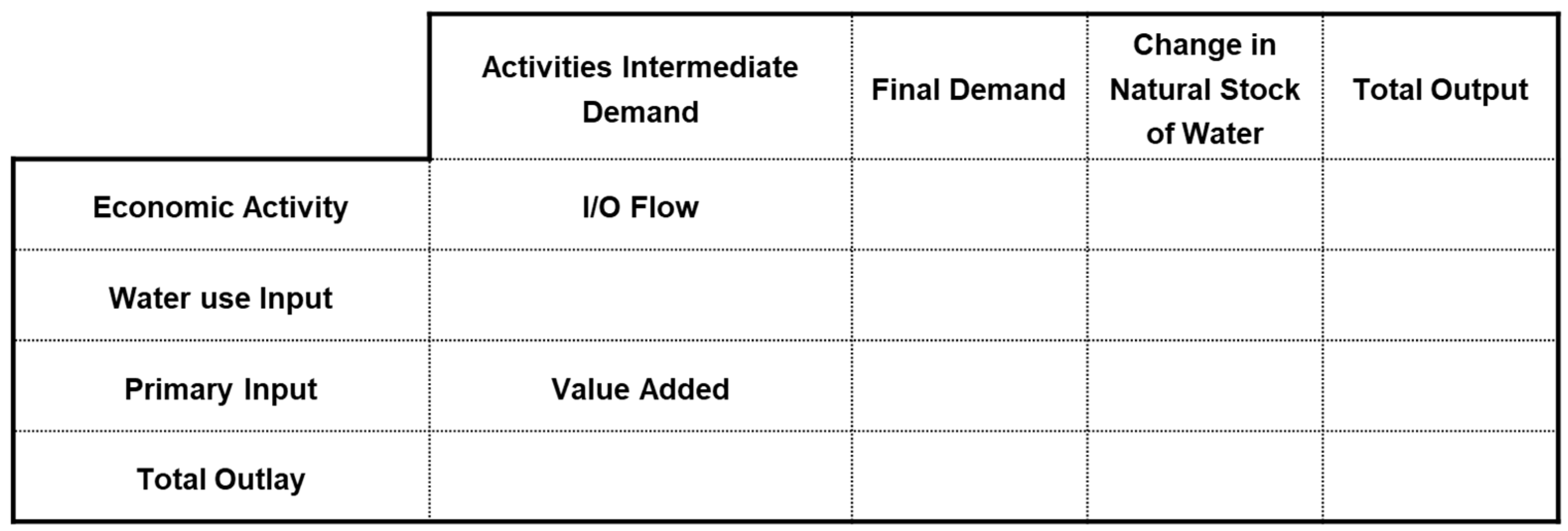
The WIOLP model constitutes an optimization framework under water use constraints based on economic input–output relations. Water-related activities within economic sectors function as value flows, linking water use with industry value added. Water use also reflects the changes in both production activities and natural storage by sector, showing how constraints propagate inter-industrial ripple effects. This relationship is structurally represented by the water input–output table in Figure 1.

This table combines production and consumption flows of the conventional input–output table with water use components, systematically illustrating correlations among economic activities, water inputs, primary inputs, and gross outputs. IO models formally express the interdependence among economic sectors. The technical coefficients in the input–output table represent the direct effects of production, indicating the input required from other industries to produce one unit of output. Converting matrix A into the Leontief inverse matrix models the relationship between the final demand and sectoral output in complex structures, expressed algebraically as shown in Equation (1):

$$\mathrm{A}\mathrm{X}+\mathrm{Y}=\mathrm{X}$$

(1)

where A = [${\mathrm{a}}_{\mathrm{i}\mathrm{j}}$] the matrix of technical coefficients; X = the column vector of sectoral output; and Y = the column vector of the total final demand.

When the input–output table exists, changes in an industry’s final demand allow the prediction of impacts on overall sectoral output, analytically expressed as Equation (2):

$$\mathrm{X}={(\mathrm{I}-\mathrm{A})}^{-1}\mathrm{Y}$$

(2)

where ${(\mathrm{I}-\mathrm{A})}^{-1}$ = the Leontief inverse matrix, which quantifies the interdependence among industries and measures the direct and indirect effects of changes in final demand on the total output.

Equation (2) represents the conventional Leontief input–output identity and is introduced to describe the interdependence between the sectoral output and final demand in the standard IO framework. The WIOLP optimization model utilized in this study explicitly defines the sectoral gross output vector X as the primary decision variable. The model does not conceptualize the final demand as an exogenous driver; rather, it directly determines the feasible level of production for each industry under the resource constraints. The objective function is formulated to maximize the total value added (Z) across all sectors. This methodological framework enables the model to ascertain an optimal production and water distribution strategy that upholds economic efficiency in the face of constrained water availability. It integrates economic and water resource structures by establishing optimal water use levels per industry. The fundamental objective function of the WIOLP model is given as Equation (3):

$$\mathrm{Z}={\mathrm{V}}_{\mathrm{a}}\mathrm{X}$$

(3)

where $\mathrm{Z}$ = the total value added; ${\mathrm{V}}_{\mathrm{a}}$ = the row vector representing the total value added per unit output (KRW for economic sectors, KRW/m³ for water use sectors); and X = the column vector of the total output per sector (KRW for economic sectors, m³ for water use sectors).

In the WIOLP formulation, the sectoral output vector X is the primary decision variable. The optimization model directly determines the feasible level of production for each industry under water use constraints. Accordingly, the WIOLP model is formulated as a linear programming problem in which sectoral output levels are optimized subject to production bounds and water availability constraints.

The final demand is not treated as an independent optimization variable; instead, it is derived after optimization through the accounting relationship $\mathrm{Y}=(\mathrm{I}-\mathrm{A})\mathrm{X}$. This formulation avoids circular dependency between the output and final demand, ensuring a mathematically consistent optimization structure. It is important to note that water is not incorporated as a value-added generating sector within the objective function; instead, it functions as a critical resource constraint that limits the production capacity of each industry. The economic value of water is therefore determined endogenously as the shadow price, representing the marginal productivity of water under scarcity.

Water use constraints limit industry output and water consumption, forming a competitive structure while maintaining interdependence. Each sector requires water as an input element, calculated from the technical coefficient matrix A. The lower and upper limits of the water use constraint are defined in Equations (4) and (5). The lower limit (${\mathrm{X}}_{\mathrm{m}\mathrm{i}\mathrm{n}})$ represents the minimum production level below which each industrial sector cannot sustain its activities, while the upper limit (${\mathrm{X}}_{\mathrm{m}\mathrm{a}\mathrm{x}})$ represents the maximum production capacity achievable under technical and physical constraints. These equations ensure that production in each sector remains within the water use limits, enabling a quantitative analysis of the tradeoff between economic growth and water availability.

$$\mathrm{X}\ge {\mathrm{X}}_{\mathrm{m}\mathrm{i}\mathrm{n}}$$

(4)

$$\mathrm{X}\le {\mathrm{X}}_{\mathrm{m}\mathrm{a}\mathrm{x}}$$

(5)

where ${\mathrm{X}}_{\mathrm{m}\mathrm{i}\mathrm{n}}$ = the minimum production level required to sustain essential sector activities (KRW for economic sectors, m³ for water use sectors); and ${\mathrm{X}}_{\mathrm{m}\mathrm{a}\mathrm{x}}$ = the maximum attainable production within the technical and physical limits.

In general, the national economy consists of n industrial sectors. The water use of each sector is expressed by the water use constraint in Equation (6). The coefficient ${\mathrm{w}}_{\mathrm{i}}$ for each industry i represents the water required per unit of output for production activities. The sum of water use across all sectors, plus household water use, cannot exceed the total available water resources ${\mathrm{W}}_{\mathrm{m}\mathrm{a}\mathrm{x}}$. This relationship is defined as Equation (6):

$$\sum _{\mathrm{i}=\mathrm{l}}^{\mathrm{n}}{\mathrm{w}}_{\mathrm{i}}{\mathrm{X}}_{\mathrm{i}}+{\mathrm{W}}_{\mathrm{h}\mathrm{o}\mathrm{u}\mathrm{s}\mathrm{e}\mathrm{h}\mathrm{o}\mathrm{l}\mathrm{d}}\le {\mathrm{W}}_{\mathrm{m}\mathrm{a}\mathrm{x}}$$

(6)

where ${\mathrm{w}}_{\mathrm{i}}$ = the water use coefficient for sector i (m³ per unit of output); ${\mathrm{X}}_{\mathrm{i}}$ = the output of sector i; ${\mathrm{W}}_{\mathrm{h}\mathrm{o}\mathrm{u}\mathrm{s}\mathrm{e}\mathrm{h}\mathrm{o}\mathrm{l}\mathrm{d}}$ = the household water requirement; and ${\mathrm{W}}_{\mathrm{m}\mathrm{a}\mathrm{x}}$ = the total available water resources.

Maintaining the total water use for economic and domestic activities within feasible limits ensures a balance between production and resource sustainability. Finally, the non-negativity constraint of the WIOLP model indicates that the output for each industry cannot be negative, ensuring physical and economic validity by keeping outputs at practical levels. This relationship is defined as Equation (7):

$$\mathrm{X}\ge 0$$

(7)

To incorporate water availability into the WIOLP model, sectoral water consumption data were integrated with the input–output table by matching water use statistics with the corresponding industrial sectors. Water use coefficients were calculated as the ratio of sectoral water consumption to total sectoral output and incorporated into the model as resource constraints. Together, these constraints define a linear programming optimization problem that determines the optimal sectoral output levels under limited water availability while maintaining the structural interdependence of industries represented in the input–output system.

2.3. Calculation of the Input–Output Table and Water Use

The input–output table is a comprehensive statistical matrix that records transactional relationships of goods and services produced by each industry within the national economy. In Republic of Korea, the table is prepared every 5 years, and the extended table is updated annually [49,50]. This study applied the 2015 and 2018 input–output tables based on nominal prices to analyze drought damage in the corresponding years.

Because the official input–output tables are compiled in nominal prices, this study also used nominal price-based tables in the analysis. Since the objective of this study is to examine drought events occurring in specific years rather than conducting a long-term intertemporal comparison, the use of nominal prices does not significantly affect the interpretation of the results. Nevertheless, the potential influence of inflation on intertemporal comparability is acknowledged as a limitation of the study.

The actual economic scale was assessed during comparison and analysis to reflect real changes in the economy. Water use data were categorized into three categories: domestic, industrial, and agricultural. These data were compiled from statistics provided by the Ministry of Environment and the Ministry of Data and Statistics. Agricultural water was divided into paddy, field, and livestock water, while industrial water was divided into 24 sectors. Domestic water included household, business, and general uses. These data provided the basis for analyzing the water use structure of industrial sectors.

Industrial classification was reorganized for consistency between the industrial classification of the input–output table and the classification system of water use statistics. The aggregation was conducted by considering similarities in economic activities, production structures, and water use characteristics among industries, rather than by applying statistical clustering techniques.

The conventional input–output table comprised 33 industrial sectors, but water use data for some industries were unavailable; therefore, industrial sectors with similar water use patterns were consolidated in this study based on water use characteristics and data availability. Through this process, 33 industrial sectors were reclassified into 17 sectors.

Table 3. Reclassification of the industrial classification and water usage.

IO Code	Industry Classification	WU Code	Water Usage
A	Agricultural, forestry, and fisheries products	A	Agricultural, forestry, and fisheries products
B	Mineral products
C01	Food and beverage	B	Food and beverage
C02	Textiles and leather goods	C	Textiles and leather goods
C03	Wood and paper, printing	D	Wood and paper, printing
C04	Coal and petroleum products	E	Coal and petroleum products
C05	Chemical products	F	Chemical products
C06	Nonmetallic mineral products	G	Nonmetallic mineral products
C07	Primary metal products	H	Primary metal products
C08	Metal-processed products	I	Metal-processed products
C09	Computer, electronic, and optical instruments	J	Computer, electronic, and optical instruments
C10	Electrical equipment	K	Electrical equipment
C11	Machinery and equipment	L	Machinery and equipment
C12	Transportation equipment	M	Transportation equipment
C13	Other manufacturing products	N	Other manufacturing products
C14	Manufacturing toll processing and repairing industrial equipment	O	Manufacturing toll processing and repairing industrial equipment
D-T	Service industries	P	Services
		Q	Living water

Data from the Economic Statistics System of the Bank of Korea (ECOS; https://ecos.bok.or.kr, accessed on 1 May 2025).

presents the correspondence between industrial sectors and water use classification, establishing a consistent framework for incorporating correlations between economic activities and water use by industry within the WIOLP model.

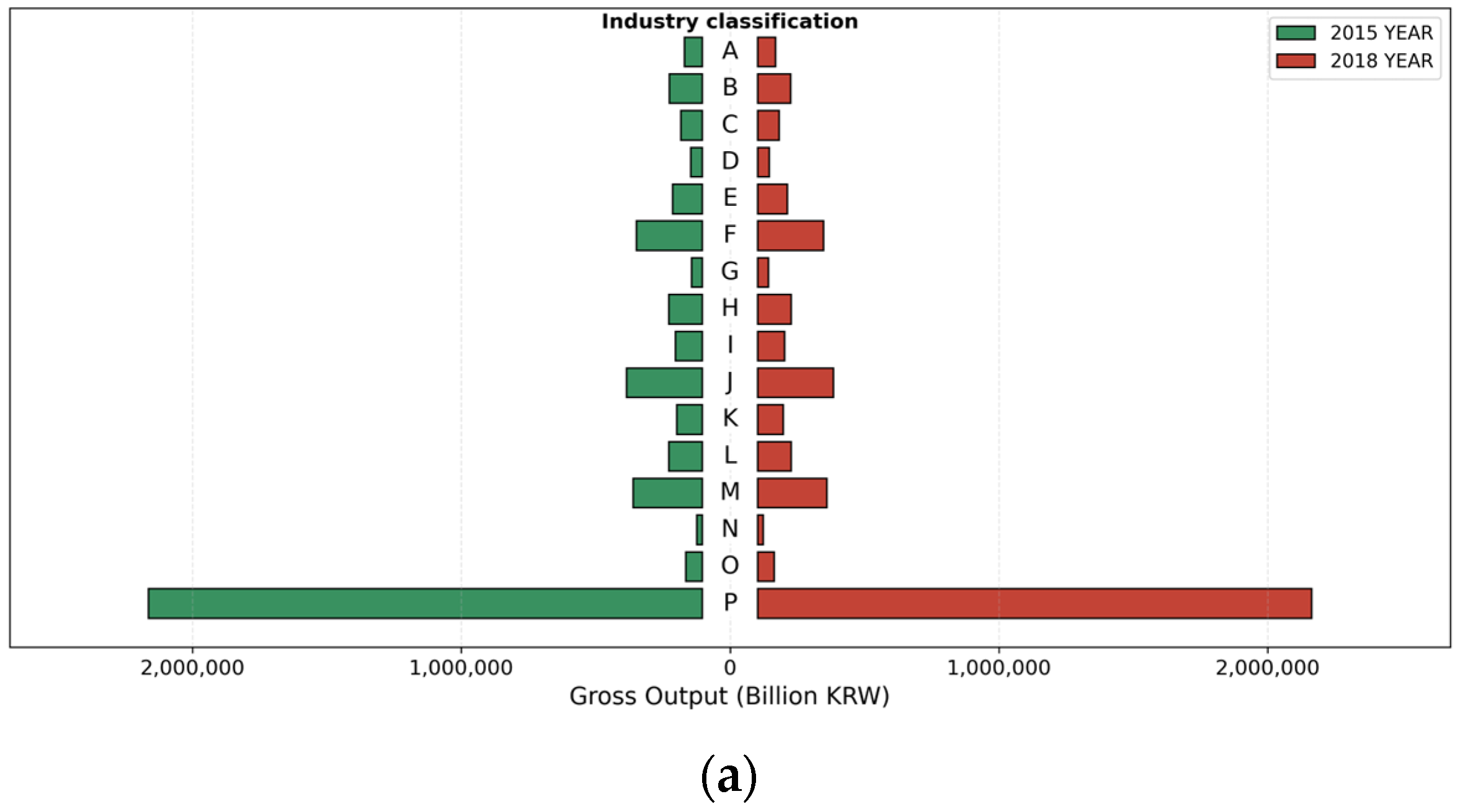
For the 17 reclassified sectors, the gross output and water use data for 2015 and 2018 were constructed. The input–output table utilized the national transaction table that reflects the domestic production structure, yielding 3,833,562 billion KRW in 2015 and 4,336,564 billion KRW in 2018. 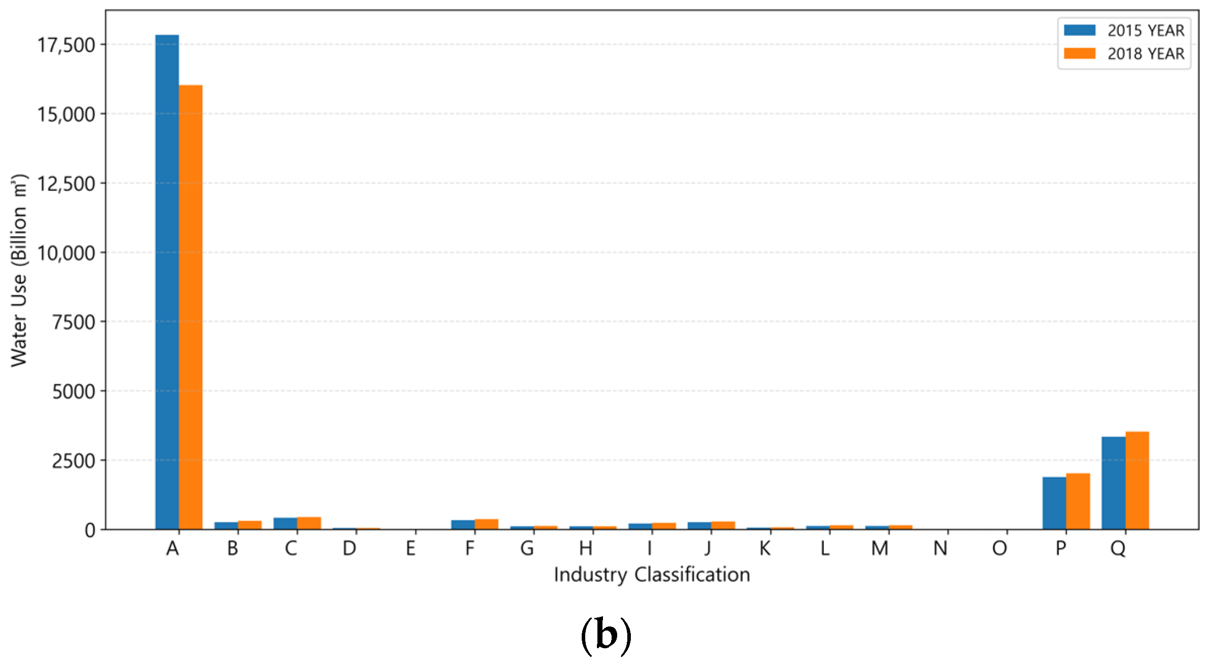By industry, the service sector exhibited the highest gross output, approximately 2,000,000 billion KRW, while other sectors ranged from 20,000 to 300,000 billion KRW (Figure 2a). Water use by industry was calculated for 18 items, including domestic water (Figure 2b).

Total water use decreased from 25,205 billion m³ in 2015 to 23,959 billion m³ in 2018. Agricultural water accounted for approximately 70% of the total water use in Republic of Korea. Due to national development and reduced agricultural area, agricultural water declined by 10% and total water use by 5%. By contrast, industrial and service sector water use increased by 3% to 20% in 2018. These changes reflect a structural shift in water use patterns during the 2018 drought, demonstrating a shift from agriculture-focused to industry- and service-oriented water allocation. These data provide a basis for reflecting industry-specific water use changes under WIOLP model constraints.

The WIOLP model was analyzed as a linear program using Python (version 3.12). The SciPy Simplex solver was employed as the analysis library. Because the model is linear, the solver guarantees convergence to a global optimum when a feasible solution exists. Water availability scenarios were generated by progressively reducing the water constraint parameter ${\mathrm{W}}_{\mathrm{m}\mathrm{a}\mathrm{x}}$ while maintaining all other structural parameters as constants.

3. Results and Analysis

3.1. Input–Output Analysis Under the Application of the WIOLP Model

The WIOLP model was applied to 2015 and 2018 to analyze the impacts of drought-induced water use constraints on inter-industry economic ripple effects. By integrating the input–output table and water use data, the model reflects the interdependence between production activities and water use by industry, enabling a quantitative assessment of the changes in productivity and value added when water constraints occur. The analysis followed a three-stage procedure: First, 100% water use was set under the reference scenario to calculate the gross output and value added by industry. Second, water use was reduced by 10% under constraint scenarios to assess stepwise impacts on production. Third, socioeconomic potential losses were estimated by comparing constraint scenarios with the reference scenario. In this section, the relationship between the production structure and water use under 100% water use is analyzed.

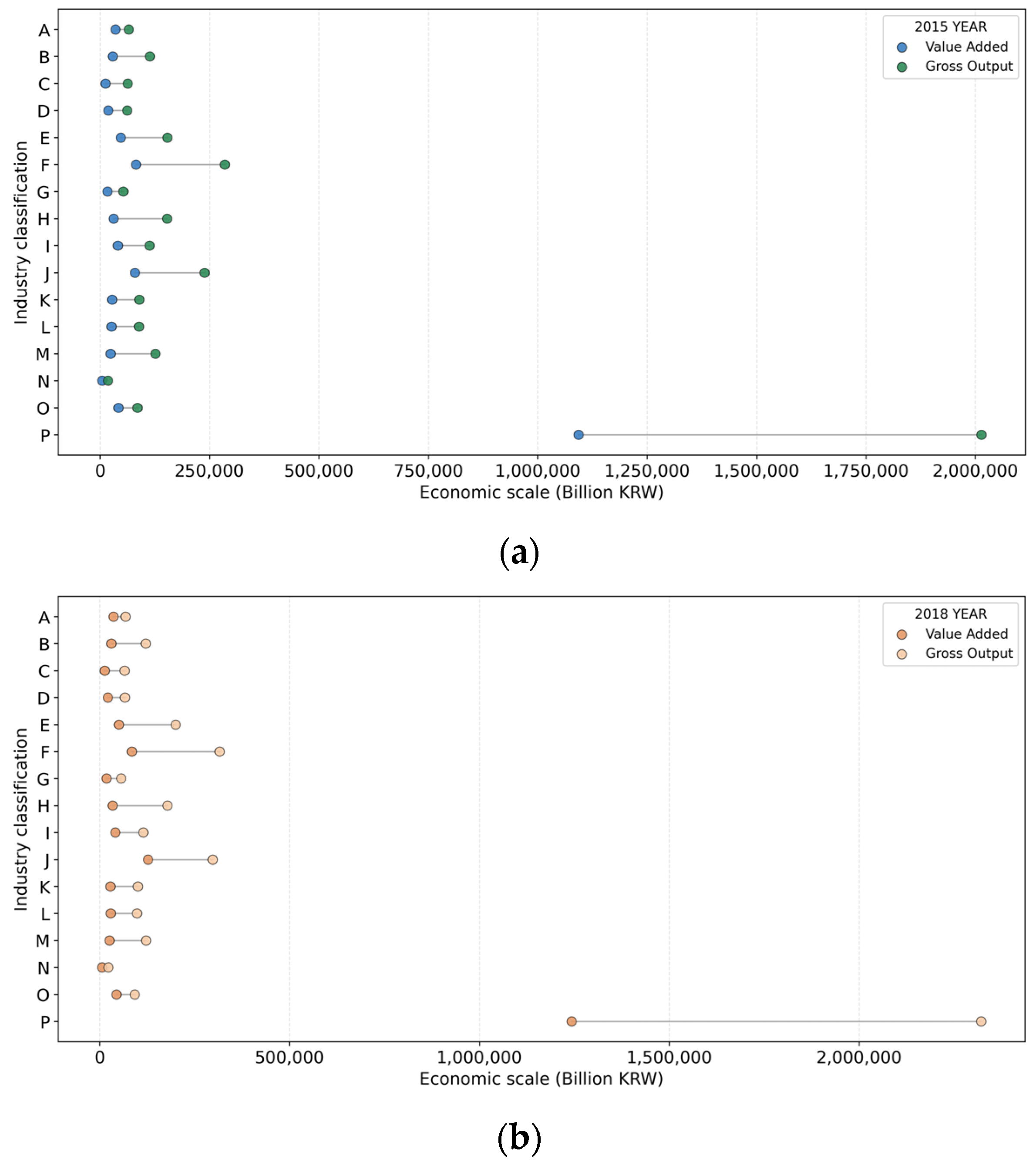
The WIOLP model is based on Equations (1)–(3). The technical coefficient matrix identifies the inter-industrial input–output structure, while the Leontief inverse matrix quantifies the direct and indirect effects of the changes in final demand on sectoral output. Ripple effects of water use on the overall economic production system are structurally analyzed by setting the functional relationship between water use and value added for each industry. The objective function (Equation (3)) maximizes the total value added by considering the value-added rate per unit of output for each industry. Upon the complete utilization of the supplied water, the WIOLP model estimated total output for 2015 at 38.33562 trillion won, with a value added estimation of 16.374507 trillion won. The total output in 2018 was estimated at 42,402,689 million won, and the value added was estimated at 18,734,012 million won. The distributions of gross output and value added by industry are presented in Figure 3.

In both 2015 (Figure 3a) and 2018 (Figure 3b), the service sector (P) exhibited the largest production scale among all industries, representing approximately 45–50% of domestic gross output. The manufacturing sectors (B to O) demonstrated clear production inducement effects due to the high ratio of gross output to value added. In particular, the gross output and value added increased in 2018 for the electricity and electronics sectors (J and K) as well as the machinery sectors (L and M), indicating a shift toward a more technology-intensive structure. The agriculture, forestry, and fisheries sectors (A) account for 70% of total water usage. However, the value added is less than 2% of the total amount, indicating a high dependence on water and low economic efficiency. This imbalance indicates that agricultural sectors may be the most vulnerable to physical impacts, such as drought.

3.2. Socioeconomic Value Assessment According to Reduced Water Use

In this section, the impacts of water use constraints on socioeconomic potential losses across industries were quantitatively assessed based on the gross output and value added by industry, as calculated in Section 3.1 during the second stage of the WIOLP analysis. To simulate increasing levels of water scarcity, the total available water resource parameter ${\mathrm{W}}_{\mathrm{m}\mathrm{a}\mathrm{x}}$ in the water constraint was gradually reduced from 100% to 10% of the baseline water availability. At each reduction step, the WIOLP model was solved to determine the optimal sectoral output levels under the corresponding water availability condition, while maintaining the sectoral minimum production constraints and other structural parameters as constants.

Water use reductions from 100% to 10% were applied using WIOLP constraints (Equations (4)–(7)), and socioeconomic potential losses and shadow prices were calculated according to the reduction in production activities at each step. The shadow price of water was obtained from the dual variable associated with the total water availability constraint (Equation (6)) in the WIOLP optimization model. This value represents the marginal increase in total economic value added resulting from an additional unit of available water. The analysis focused on 2015 and 2018 when drought damage occurred.

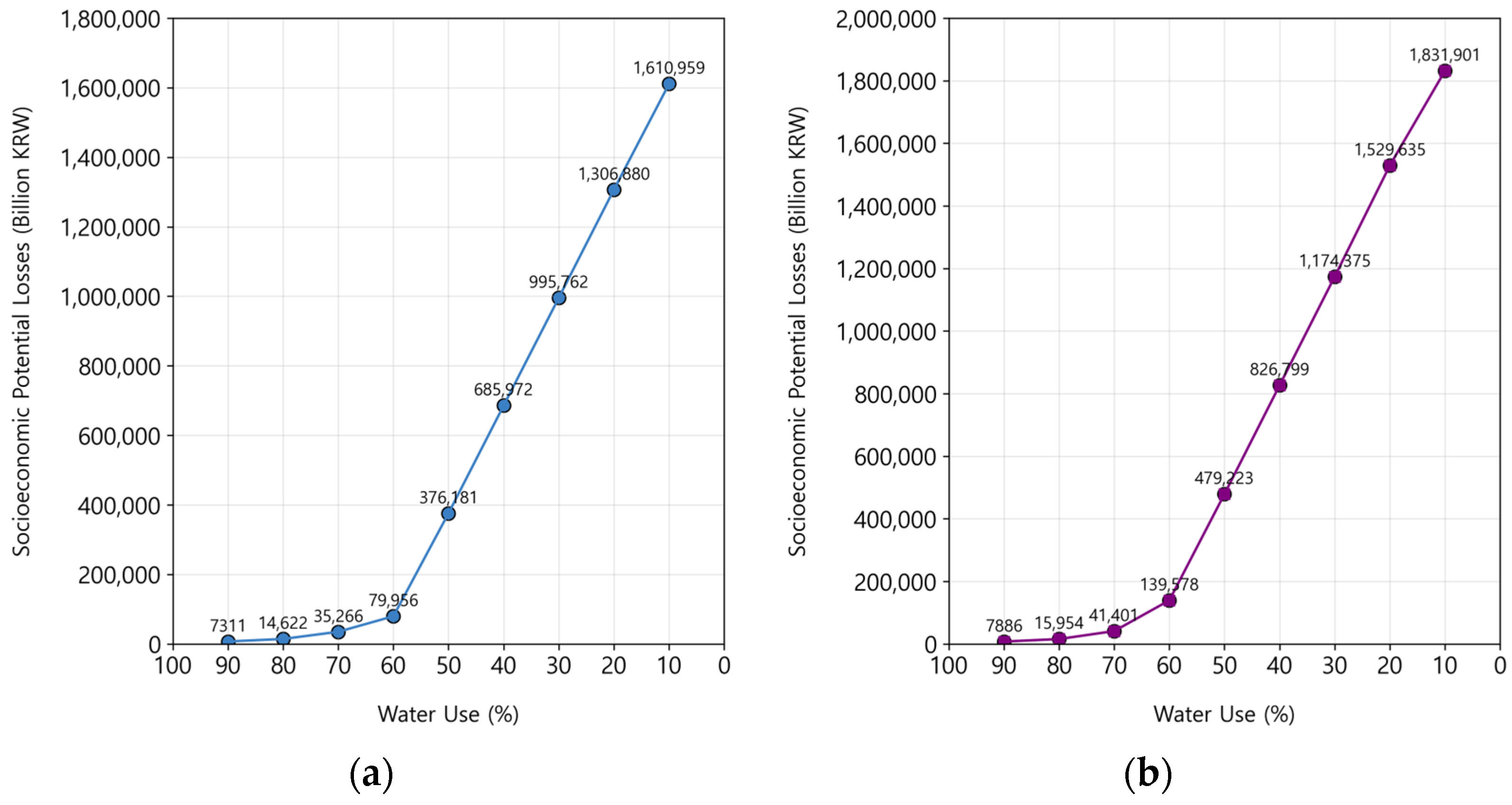
In 2015, socioeconomic potential losses ranged from 7311 to 799,560 billion KRW as water use decreased from 90% to 60%. Losses escalated rapidly when water use fell below 50%. Between 50% and 10%, losses increased by approximately 300,000 billion KRW at each level. The maximum potential loss was 311,118 billion KRW when water use fell from 30% to 20%. This demonstrates a nonlinear increase. This occurs when water-intensive sectors reach their minimum production levels (${\mathrm{X}}_{\mathrm{m}\mathrm{i}\mathrm{n}}$), which causes a rapid contraction of the feasible production region and a cascading economic effect (Figure 4a).

The nonlinear increase in socioeconomic potential losses observed below approximately 50% water availability arises from the tightening of the water constraint in the WIOLP model. As the water availability constraint becomes binding, several water-intensive sectors approach their minimum production levels, causing a rapid contraction of the feasible production region and resulting in disproportionately larger economic losses.

The 2018 analysis exhibited a similar trend in socioeconomic potential losses. When water use decreased from 90% to 70%, losses per step rose from 7886 to 41,401 billion KRW. A decrease from 70% to 60% resulted in losses of 98,177 billion KRW, and when water use fell below 60%, each step incurred approximately 330,000 billion KRW in losses. Notably, the reduction from 30% to 20% produced a maximum loss of 355,260 billion KRW, reflecting a larger loss scale compared to 2015 (Figure 4b).

The estimated socioeconomic potential losses represent cumulative economy wide reductions in outputs resulting from water availability constraints. When compared with national GDP, these losses correspond to a significant but interpretable share of the total economic activity, reflecting the cascading inter-industry effects captured in the input–output framework.

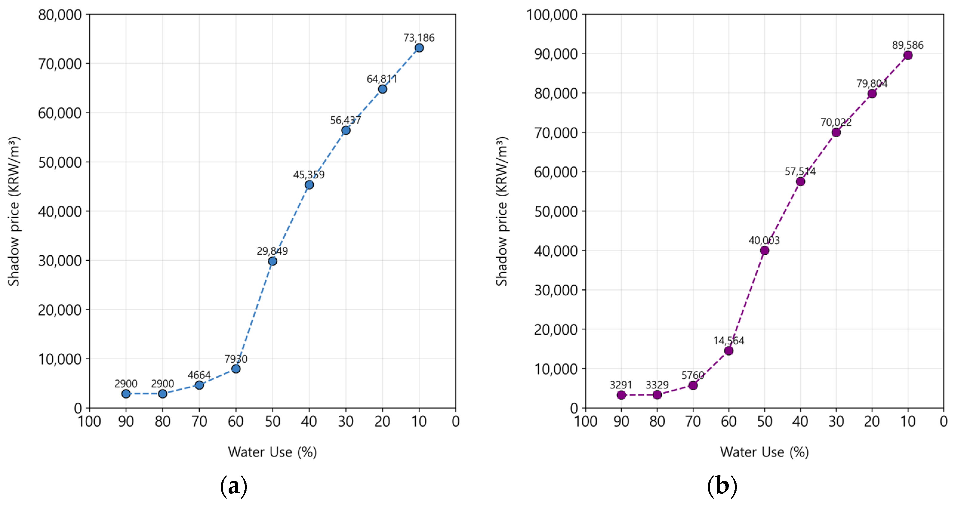
These results indicate nonlinear threshold impacts, where inter-industrial ripple effects surge as water use declines beyond certain levels. In other words, water use constraints generate threshold effects on productivity, employment, and value added beyond a simple proportional reduction in production. Figure 5 presents the shadow price per m³ due to reduced water use. In 2015, the shadow price increased from 7311 to 73,186 KRW/m³, with a sharp rise of more than 20,000 KRW/m³ between 60% and 50% water use (Figure 5a). In 2018, the shadow price increased from 3291 to 89,586 KRW/m³, with a steep rise of approximately 25,000 KRW/m³ for the same range (Figure 5b). These patterns demonstrate that the marginal productivity of water nonlinearly increases as water constraints tighten. In other words, water serves as a key marginal input in industrial production, and its economic value (shadow price) rises exponentially under stricter constraints. These results confirm that the WIOLP model efficiently quantifies both inter-industry ripple effects and marginal water values under scarcity.

3.3. Assessment of the Effects of Reduced Water Use on Each Industry

This section quantitatively analyzed the effects of reduced water use on gross output by industry, constituting the third stage of the WIOLP analysis. Industries were classified into 17 sectors based on the input–output table and water use data. For each industry, the gross output change rate was calculated at 10% water use reduction intervals to evaluate the water dependence and threshold levels.

Table 4. Sectoral economic output by industry of reduced water use in 2015.

Water Use (%)	$\mathbf{Sectoral} \mathbf{Economic} \mathbf{Output} \mathbf{(}{10}^3 \mathbf{Billion} \mathbf{KRW}\mathbf{)}$
	A	B	C	D	E	F	G	H	I	J	K	L	M	N	O	P
100	66	114	63	61	154	285	53	153	113	239	90	89	126	18	86	2013
90	57	112	63	61	153	284	53	153	113	239	89	89	126	18	85	2011
80	47	111	63	61	153	283	53	153	113	239	89	89	126	18	85	2009
70	39	79	63	60	152	281	53	152	112	239	89	89	126	18	84	1999
60	-	54	28	58	151	275	34	151	111	238	89	88	125	18	78	1973
50	-	43	-	27	141	254	27	62	102	233	83	84	121	16	71	1539
40	-	-	-	20	131	236	20	55	94	227	77	81	117	13	67	-
30	-	-	-	-	120	218	14	48	86	221	70	77	112	11	63	-
20	-	-	-	-	104	-	-	40	76	214	64	71	108	9	-	-

“-” indicates negligible or effectively zero sectoral output under the corresponding water availability scenario.

shows the gross output changes in 2015.

Production in industry A (agricultural, forestry and fisheries products) ceased at 40% water use. Industry C (textiles and leather goods) halted at 50%; industries B (food and beverage) and D (Wood and paper, printing) at 60%; and industries E (coal and petroleum products), F (chemical products), G (nonmetallic mineral products), and O (manufacturing toll processing and repair of industrial equipment) at 70%. A sharp output reduction occurred across industries at 70% or lower water use, particularly in primary and secondary sectors with high water dependence (e.g., agriculture, mining, manufacturing, construction). By contrast, industries E (coal and petroleum products), H (primary metal products), J (computer, electronics, optical instruments), K (electrical equipment), L (machinery and equipment), M (transportation equipment), and N (other manufacturing) maintained some production even at 50% water use, indicating these are service-oriented sectors with lower water reliance.

Table 5. Sectoral economic output by industry of reduced water use in 2018.

Water Use (%)	Sectoral Economic Output (Trillion KRW)
	A	B	C	D	E	F	G	H	I	J	K	L	M	N	O	P
100	68	121	65	67	200	316	57	178	115	297	100	98	122	23	92	2322
90	58	120	65	66	200	315	57	178	115	297	100	98	122	23	92	2319
80	48	118	65	66	200	314	56	178	114	297	100	98	121	23	91	2316
70	38	79	65	65	199	311	56	177	114	297	100	98	121	23	90	2302
60	-	57	21	35	195	299	34	88	110	295	98	96	120	22	80	2238
50	-	46	16	27	174	100	28	60	53	289	92	90	116	20	68	1808
40	-	-	-	20	161	79	21	52	44	282	84	86	110	17	63	-
30	-	-	-	-	147	-	13	43	-	276	77	83	105	14	58	-
20	-	-	-	-	134	-	-	30	-	267	67	78	71	-	-	-

“-” indicates negligible or effectively zero sectoral output under the corresponding water availability scenario.

presents the 2018 results. Industry A halted at 40% water use; industries B, C, and P (services) at 60%; industries D, F, and I (metal-processed products) at 70%; and industries G and N at 80%. Overall water dependence increased in 2018 due to higher evapotranspiration and agricultural water scarcity despite near-normal precipitation; consequently, gross output losses were higher in 2018 at equivalent water reduction levels. A comparison of 2015 and 2018 shows that industries A, B, C, D, F, G, I, N, and O were the most sensitive to water reductions, representing water-intensive sectors including agriculture, forestry, mining, manufacturing, and construction. Water constraints directly delayed production in these sectors. Conversely, industries E, H, J, K, L, and M maintained more than 90% of gross outputs at 50% water use or less, classifying them as water-independent. These results align with the socioeconomic potential loss and shadow price analyses in Section 3.2, indicating that water constraints disproportionately affect water-intensive industries rather than the entire economy evenly.

4. Discussion

In this study, socioeconomic potential losses resulting from drought-induced water use constraints and inter-industrial ripple effects were quantitatively identified using the WIOLP model. When comparing 2015 and 2018, socioeconomic potential losses increased nonlinearly once water use decreased to 50% or less [6,8,25]. The analysis results revealed interdependence between industries and identified a critical point for potential socioeconomic losses. This outcome contrasts with the linear proportional relationships observed in previous input-output analysis studies.

Previous studies analyzed drought-induced economic ripple effects through IO models or computable general equilibrium (CGE) models, but most could not fully capture inter-industry interdependence because water use was treated as an exogenous variable [21,26]. In this study, the WIOLP model analyzed the optimization relationship between production activities and water use by including water use constraints as endogenous variables. Based on this, the shadow price under limited water use and the nonlinear loss structure resulting from reduced water use, which previous studies could not capture, were quantitatively identified.

According to the WIOLP model results, the maximum socioeconomic potential losses were 311,118 billion KRW in 2015 and 355,260 billion KRW in 2018 when water use decreased by 10% per step, exceeding the loss rates reported in previous studies [9,13]. This outcome reflects the empirically examined nonlinear ripple effects underestimated in conventional IO and CGE models, accounting for accumulated inter-industry effects. Compared to a GDP loss of approximately 5% during drought reported in a previous study [25], the results show that economic impact increases exponentially as inter-industry interdependence intensifies. This trend is also confirmed by shadow price analysis, where the shadow price approximately doubled or tripled when water use decreased from 60% to 50%.

Previous studies reported the agricultural sector as representing a dominant proportion of water use and the largest economic loss during drought [2,12]. The WIOLP model results of this study confirm the structural vulnerability, as production in industry A (Agricultural, forestry, and fisheries products) ceased when water use fell to 40% or less. In addition, the sharp rise in the shadow price indicates a rapid increase in the marginal economic value of water by industry. These findings suggest that future policies should shift from simple demand reduction to differentiated water supply management systems that account for water dependence and marginal values by industry [15,28]. The WIOLP model outputs can serve as a policy simulation tool to assess the economic effects of drought-response strategies and guide priorities for water distribution while strengthening economic resilience.

5. Conclusions

This study applied the WIOLP model to quantitatively identify socioeconomic potential losses in the national economy caused by drought-induced water use constraints and inter-industry ripple effects. The model integrates input–output tables and water use data to analyze both the optimization of production activities by industry and economic ripple effects under limited water use conditions.

The analysis revealed that water use constraints nonlinearly increased socioeconomic potential losses due to inter-industry interdependence. Losses for each industry sharply increased beyond critical thresholds when water use decreased below certain levels, unlike the linear assumptions of conventional IO or CGE models. While industries with high water use (e.g., agriculture, forestry, fisheries, chemicals, and non-metals) showed significant potential losses, the electricity, electronics, and machinery industries exhibited relatively low potential losses, highlighting that differences in water dependence drive economic vulnerability. While the analysis is chiefly concerned with the short-term economic impacts of drought-induced water shortages, the results also furnish significant insights into the potential long-term socioeconomic implications of water scarcity at the national level. The findings emphasize the structural vulnerabilities of water-dependent industries and the propagation of water scarcity effects across interconnected sectors.

Although the analysis primarily captures the short-term economic impacts of drought-induced water shortages, the results also provide important insights into the potential long-term socioeconomic implications of water scarcity at the national level. In particular, the findings highlight structural vulnerabilities of water-dependent industries and the propagation of water scarcity effects across interconnected sectors.

The WIOLP model addresses the limitations of conventional IO and CGE models by integrating water use as an endogenous constraint, reflecting interactions between industries under resource limitations more realistically. This approach allowed the quantitative identification of structural ripple effects during water crises, demonstrating that water scarcity can be expressed as an economic variable via shadow price calculations. The study demonstrates the empirical potential of the WIOLP model for drought response and water resource management. Future research will expand the model to a multi-regional input–output framework to trace water scarcity risk propagation between regions and combine climate change scenarios (AR6) to assess the economic impacts of future water scarcity.