Hybrid Physical–Machine Learning Soil Moisture Modeling at Orchard Scale in Irrigated Citrus Orchards Using Sentinel 1 and 2 and Agroclimatic Data

Abstract

Accurate orchard-scale soil moisture information is a key requirement for efficient irrigation management in perennial crops such as citrus orchards, particularly in Mediterranean environments characterized by water scarcity and strong spatial and temporal variability in soil moisture, canopy structure, and irrigation scheduling. This study proposes a hybrid physical–machine learning methodology for soil moisture estimation that integrates in situ capacitance sensor measurements, Sentinel-1 SAR observations, Sentinel-2 optical imagery, and ERA5-Land agroclimatic variables. Physically based soil moisture estimates were first obtained through the inversion of Sentinel-1 backscatter using integral equation scattering models, a physically based soil dielectric model, and a simplified vegetation attenuation scheme. These physically derived estimates were subsequently incorporated as predictors within supervised machine learning models, together with multi-source remote sensing and meteorological variables. Several algorithms were evaluated, including regularized linear models, support vector regression, random forests, and gradient boosting methods. Model performance was assessed using a strict interannual validation strategy based on independent-year predictions to ensure robust generalization. Within this methodology, tree-based ensemble models achieved the highest and most consistent performance at the orchard scale, with coefficients of determination ranging from 0.55 to 0.76 and root mean square errors typically between 0.7 and 1.1% volumetric soil moisture in the best-performing cases. Benchmarking against a physical-only baseline demonstrated that the hybrid methodology consistently reduced prediction errors and improved temporal robustness under independent-year validation. Overall, the results demonstrate that hybrid physical–machine learning approaches provide a robust and scalable solution for orchard-scale soil moisture monitoring in irrigated citrus orchards using operational data streams, supporting advanced irrigation management and precision agriculture applications in Mediterranean perennial cropping systems.

1. Introduction

Traditional approaches to soil moisture monitoring rely on in situ sensors, such as capacitance or frequency domain reflectometry (FDR) probes, which provide high temporal resolution measurements but are spatially limited and costly to deploy at scale. As a result, their use is often restricted to a small number of reference points, which may not adequately represent the spatial heterogeneity of soil moisture within and between agricultural orchards. This limitation has motivated increasing interest in remote sensing techniques to complement ground-based observations and enable spatially explicit soil moisture monitoring over agricultural areas.

Microwave remote sensing, particularly Synthetic Aperture Radar (SAR), has long been recognized as a powerful tool for soil moisture retrieval due to its sensitivity to the dielectric properties of the soil and its ability to operate independently of solar illumination and cloud cover, while acknowledging that satellite-based observations are primarily sensitive to near-surface soil layers [1,2,3]. The launch of the Sentinel 1 mission has significantly enhanced the potential for operational soil moisture monitoring at high spatial and temporal resolution, especially when combined with optical information from Sentinel 2. Numerous studies have demonstrated the value of synergistic Sentinel 1 and Sentinel 2 approaches for soil moisture estimation in agricultural landscapes [4,5,6].

Physical scattering models, such as the Integral Equation Model (IEM) and its advanced formulations (AIEM, CIEM), provide a physically consistent methodology to interpret SAR observations, but their direct application is often limited by uncertainties in model parameters and by the complexity of soil–vegetation interactions [7,8,9,10]. Vegetation effects are commonly addressed through simplified representations, such as the Water Cloud Model (WCM) [11] which introduces additional parameters that require calibration and may vary across sites and seasons.

In parallel, data driven and machine learning approaches have gained increasing attention for soil moisture estimation, as they are able to capture complex and nonlinear relationships between remote sensing observations, meteorological variables, and in situ measurements [12]. When combined with ancillary information such as reanalysis-based climate data (e.g., ERA5-Land), these methods can substantially improve predictive performance and temporal continuity [13,14]. Nevertheless, purely data driven models may suffer from limited interpretability, reduced robustness outside the calibration domain, and potential overfitting if validation strategies are not carefully designed [15,16].

To address these limitations, hybrid approaches that integrate physical modeling with machine learning have emerged as a promising direction for soil moisture monitoring. By incorporating physically based estimates as predictors within data driven methodologies, such approaches aim to leverage the strengths of both paradigms: the physical consistency and transferability of scattering models, and the flexibility and predictive power of machine learning algorithms.

While hybrid methods have been explored at regional to global scales, their application and validation at the orchard scale in Mediterranean conditions, where perennial tree orchards dominate the landscape, remain relatively limited. Unlike annual crops, which typically achieve full canopy cover during the growing season, tree orchards include substantial areas of bare soil between rows. This structural configuration alters soil–plant–atmosphere interactions and increases the relative contribution of the soil component to the SAR backscatter, making soil moisture retrieval more challenging due to the combined effects of surface roughness, vegetation structure, and management practices.

From an agronomic point of view, efficient water management is a key challenge for Mediterranean agriculture, particularly in perennial crops such as citrus orchards, where irrigation decisions strongly influence yield, fruit quality, and long-term soil–plant interactions. In this context, under semi-arid and water limited conditions, soil moisture acts as a key state variable governing plant water availability and mediating crop responses to irrigation and climatic variability. Therefore, accurate and timely information on soil moisture dynamics at the orchard scale is essential to support precision irrigation strategies and sustainable water use in citrus production systems.

Reliable parcel scale soil moisture information underpins precision irrigation, water use efficiency, and climate resilient production. In Mediterranean regions facing recurrent droughts and water scarcity, operational remote sensing-based solutions can reduce monitoring costs and support evidence-based water policies. Within this context, the present study proposes a hybrid physical–machine learning methodology for orchard scale soil moisture modeling in citrus orchards, integrating in situ FDR measurements, Sentinel 1 SAR data, Sentinel 2 optical information, and ERA5-Land agroclimatic variables. Physical inversion of SAR observations using IEM-based models, combined with dielectric and vegetation representations is employed to derive physically consistent soil moisture estimates. These estimates are subsequently integrated into machine learning models, together with remote sensing indices and meteorological variables, to improve predictive performance and robustness.

The specific objectives of this study are to:

(i)

Develop a hybrid physical–machine learning methodology for orchard-scale soil moisture estimation in citrus orchards.

(ii)

Evaluate the performance and interannual generalization of different machine learning algorithms using a strict out-of-fold validation strategy.

(iii)

Assess the relative importance of input variables across algorithms to better understand the drivers of model performance.

(iv)

Quantify the added value of integrating physically based soil moisture estimates together with ancillary remote sensing and agroclimatic variables against a physical-only baseline within a data-driven modeling methodology.

2. Materials and Methods

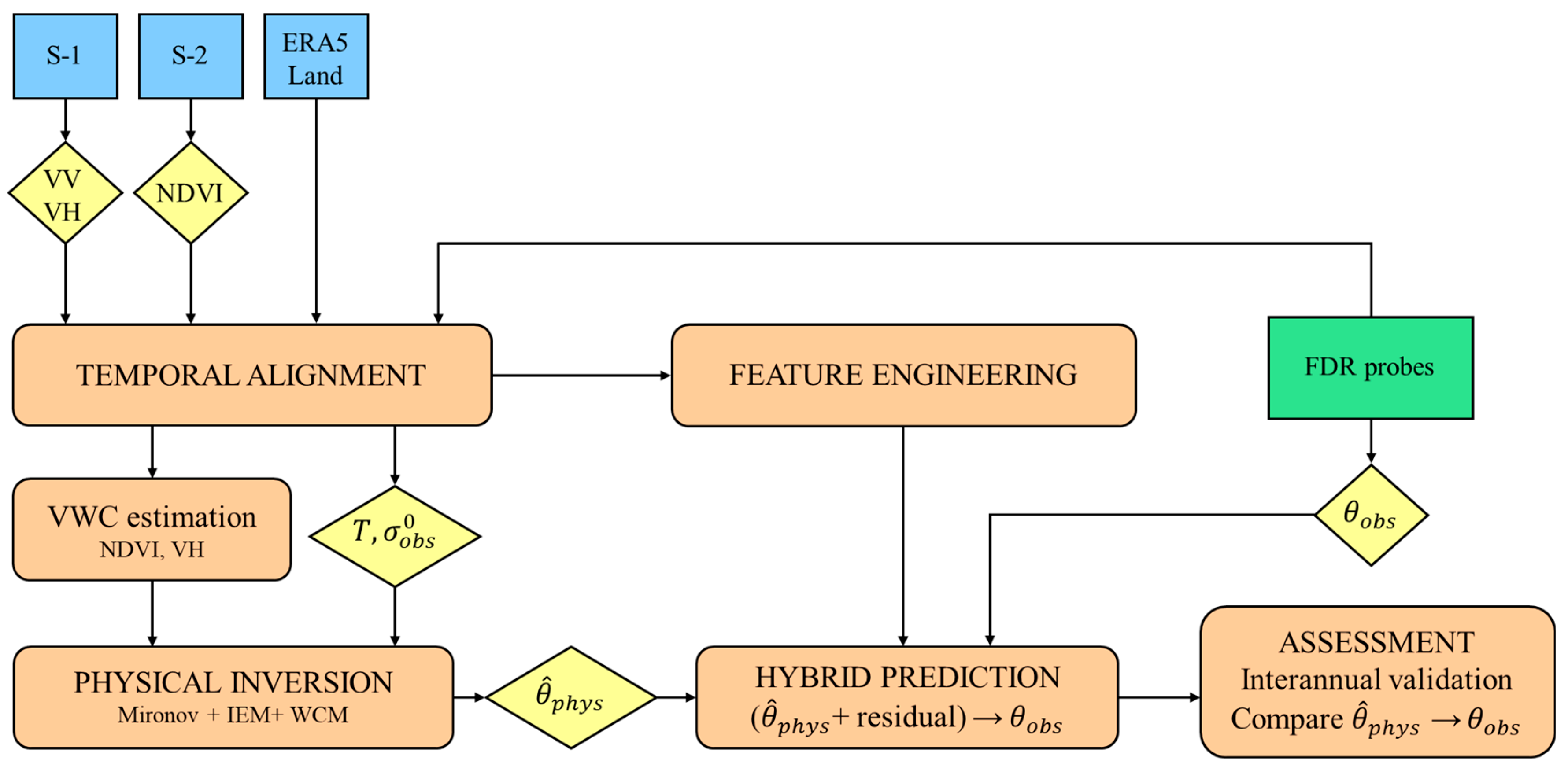
Figure 1 shows the workflow of the methodological approach carried out in the study.

2.1. Study Area

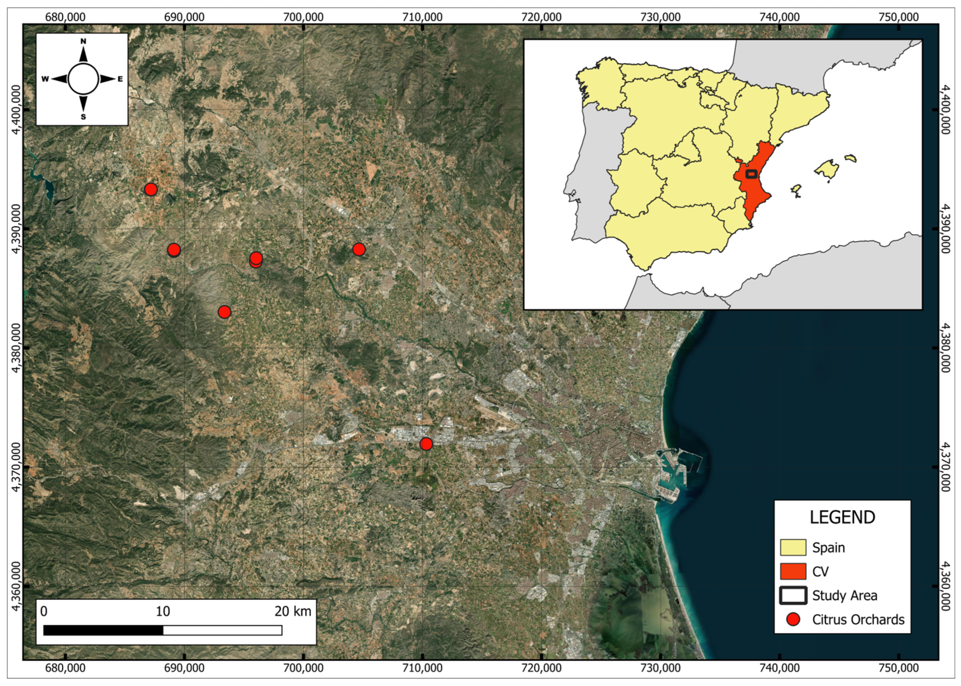
The study was conducted in 9 commercial citrus orchards representative of Mediterranean irrigated agriculture, located within a region of approximately 600 km² in the central area of the Comunitat Valenciana (CV) in eastern Spain (Figure 2) (some overlap at the scale).

Valencian citrus orchards commonly occur on calcareous (alkaline) soils with variable texture (sandy-loam to clay-loam) and often low–moderate water-holding capacity and micronutrient issues; such heterogeneity motivates physics-informed ML and strict interannual validation.

We also note that management and irrigation are known to modify soil properties in Eastern Spain, further supporting a modeling strategy that fuses SAR/optical/climate signals.

2.2. FDR Sensor Data

In these orchards, FDR probes logged volumetric soil moisture every 20–30 min at six depths (0.05–0.55 m) from 2022–2024. For modeling, we computed daily aggregates by probe and depth, which were used as ground truth and to align Sentinel 1/2 and ERA5-Land variables through the causal nearest past matching strategy. The modeling and validation emphasis was placed on soil moisture shallower than 0.35 m. This choice does not imply that the entire root system of citrus orchards is confined to this depth, as citrus roots can explore soil layers well below 1 m under favorable conditions. Instead, the focus on the upper part of the profile reflects two complementary considerations:

(i)

The highest density of fine, active feeder roots responsible for rapid water uptake generally occurs within the upper 0.3–0.6 m of soil [17];

(ii)

The sensitivity of C-band radar backscatter to volumetric soil moisture decreases with depth, especially under partial vegetation cover [18].

Consequently, predictions within the 0–0.35 m interval are expected to be most strongly correlated with both the observable signal and root water uptake dynamics.

2.3. Remote Sensing Data

Satellite data access and all subsequent preprocessing computations were conducted using the Google Earth Engine (GEE) cloud-computing platform (https://earthengine.google.com) [19]. Sentinel-1 C-band Synthetic Aperture Radar (SAR) from the Radiometrically Terrain Corrected (RTC) product (COPERNICUS/S1_GRD) was used as the primary remote sensing source for soil moisture characterization. This product provides backscatter measurements calibrated and corrected for topographic effects, minimizing geometric distortions and terrain-induced radiometric variations and ensuring temporal and spatial comparability of the backscatter signal across acquisition dates and orchards.

Backscatter coefficients (σ⁰) were obtained in both vertical–vertical (VV) and vertical–horizontal (VH) polarizations. These polarizations provide complementary information, allowing the differentiation between soil surface scattering and vegetation volume contributions. In addition, the local incidence angle was included as an auxiliary variable, as it influences the magnitude of the reflected radar signal and can modulate backscatter responses over heterogeneous terrain. Orchard-level SAR metrics were derived by spatial aggregation of pixel values within orchard boundaries, ensuring consistency within situ soil moisture observations. We note that parcel level aggregation can smooth sub parcel variability and introduce scale mismatch errors relative to point FDR measurements.

Optical multispectral information was obtained from the harmonized Sentinel-2 surface reflectance (Level 2A) product (COPERNICUS/S2_SR_HARMONIZED), which is atmospherically corrected and provide reflectance values at the surface level. These products enable direct comparison of vegetation, soil, and water reflectance across different dates and locations. A time series of Sentinel-2 images was used to compute a set of multispectral indices sensitive to vegetation vigor and water content (

Table 1. Spectral indices derived from Sentinel-2 Level-2A. For S2 Multispectral Instrument B3 is $\rho$Green, B4 is $\rho$Red, B7 is $\rho$Rededge, B8 is $\rho$NIR, B11 is $\rho$SWIR1 and B12 is $\rho$SWIR2.

Spectral Index	Formula	Description	Reference
Normalized Difference Vegetation Index (NDVI)	${\displaystyle \frac{\mathrm{B}8-\mathrm{B}4}{\mathrm{B}8+\mathrm{B}4}}$	Sensitive to vegetation vigor and greenness	[20]
Modified Normalized Difference Water Index (MNDWI)	${\displaystyle \frac{\mathrm{B}3-\mathrm{B}11}{\mathrm{B}3+\mathrm{B}11}}$	Sensitive to surface water and wetlands	[21]
Normalized Difference Moisture Index (NDMI)	${\displaystyle \frac{\mathrm{B}8-\mathrm{B}11}{\mathrm{B}8+\mathrm{B}11}}$	Sensitive to vegetation water content	Adapted from [22] *
Normalized Difference Moisture Index-2 (NDMI2)	${\displaystyle \frac{\mathrm{B}8-\mathrm{B}12}{\mathrm{B}8+\mathrm{B}12}}$	NDMI variant using SWIR2
Normalized Multi-band Drought Index (NMDI)	${\displaystyle \frac{\mathrm{B}7-(\mathrm{B}11-\mathrm{B}12)}{\mathrm{B}7+(\mathrm{B}11-\mathrm{B}12)}}$	Sensitive to soil and vegetation moisture	[23]
Normalized Multi-band Drought Index-2 (NMDI2)	${\displaystyle \frac{\mathrm{B}8-(\mathrm{B}11-\mathrm{B}12)}{\mathrm{B}8+(\mathrm{B}11-\mathrm{B}12)}}$	NMDI variant using NIR
Moisture Stress Index (MSI)	${\displaystyle \frac{\mathrm{B}11}{\mathrm{B}8}}$	Sensitive to vegetation water stress	[24]
Moisture Stress Index-2 (MSI2)	${\displaystyle \frac{\mathrm{B}12}{\mathrm{B}8}}$	MSI variant using SWIR2

* Authors referred to this index as NDWI in the original paper.

) using Google Earth Engine.

The Normalized Difference Vegetation Index (NDVI) was used to estimate vegetation water content (${VWC}_{est}$) and to account for vegetation effects on the radar backscatter signal. To ensure data quality, optical observations were filtered based on cloud probability (MSK_CLDPRB ≤ 40). As in the case of Sentinel-1, plot-level values were obtained by calculating the mean of the pixel values within the plot boundaries. All Sentinel-2-derived variables were temporally aligned with Sentinel-1 acquisitions and incorporated as auxiliary predictors in the soil moisture retrieval models.

2.4. Agroclimatic Data

Daily time series of meteorological reanalysis data (spatial resolution ≈ 9 km) provided by the European Centre for Medium-Range Weather Forecasts (ECMWF) were used. The dataset included air temperature at 2 m above the ground, daily precipitation, actual and potential evapotranspiration, and volumetric soil moisture in different soil layers (

Table 2. Variables extracted from ERA5-Land Daily.

Variable	Description
temp	Air temperature at 2 m above the surface (°C)
precip	Total daily precipitation (mm)
tevap	Total daily evapotranspiration (m)
pevap	Daily potential evapotranspiration (m)
vsm1	Volumetric soil water content in the 0–7 cm soil layer
vsm2	Volumetric soil water content in the 7–28 cm soil layer
vsm3	Volumetric soil water content in the 28–100 cm soil layer
vsm4	Volumetric soil water content in the 100–289 cm soil layer

). ERA5-Land soil moisture variables were used as large-scale hydrometeorological context rather than as direct soil moisture observations, providing information on background wetness conditions and system memory at coarser spatial scales.

2.5. Data Integration and Preprocessing

The integration of the different data sources (in situ probes, Sentinel-1, Sentinel-2, and ERA5-Land) was performed using the daily soil moisture time series from the probes as the temporal reference. Sentinel-1 observations were aggregated at the probe level and orbit, converting backscatter values from decibels (dB) to linear units, while retaining the local incidence angle and the optical indices derived from Sentinel-2.

To avoid temporal leakage Sentinel 2 indices were associated with each probe date using causal nearest past matching within a 30-day window. ERA5-Land variables were incorporated by exact daily coincidence, converting temperature to degrees Celsius and precipitation to millimeters.

Missing data was handled using a simple imputation strategy based on forward propagation from the most recent available value, avoiding the use of future information. If gaps persisted after this step, they were filled using the global median of the corresponding variable as a reference value.

2.6. Physical Modeling of Soil Moisture from SAR Data

The estimation of soil moisture from SAR observations relies on physically based inversion models whose objective is to retrieve volumetric soil moisture from the radar backscattering signal. In agricultural contexts, and particularly in perennial crops such as citrus orchards, this inversion requires disentangling the contributions of soil surface scattering and vegetation attenuation. To this end, the physical modeling methodology implemented in this study combines three main components: (i) a surface scattering model based on the Integral Equation Model (IEM), (ii) a dielectric mixing model linking soil permittivity to soil moisture and texture, and (iii) a vegetation attenuation model based on the Water Cloud Model (WCM).

In this work, a one-dimensional (1D) representation of the soil surface is assumed, implying horizontal homogeneity within the radar resolution cell and neglecting vertical variations in soil moisture within the profile. Although this simplification does not explicitly represent moisture gradients with depth, it provides a practical and widely adopted methodology for linking SAR observations to soil moisture, particularly when combined with ancillary data and hybrid modeling strategies.

Overall, this physically based scheme allows the separation of soil and vegetation contributions from the observed backscattering signal, yielding physically consistent soil moisture estimates. However, its practical application is constrained by the sensitivity of the models to parameters that are difficult to measure in situ, such as surface roughness and canopy structure. For this reason, the recent literature increasingly advocates hybrid approaches that integrate physically based estimates with machine learning techniques to improve robustness and generalization [3,6].

2.6.1. Integral Equation Model (IEM)

The Integral Equation Model (IEM) describes the radar backscattering coefficient (${\sigma }^0$) of a rough soil surface as a function of the complex dielectric permittivity of the soil ($\epsilon$), surface roughness parameters—namely, the root mean square (rms) height ($s$) and correlation length ($l$)—and the radar incidence angle (${\theta }_i$). Under conditions of small to moderate surface roughness ($k·s<3$, where $k=2\pi /\lambda$ and $\lambda$ is the radar wavelength), the backscattering coefficient for a given polarization (VV or VH) can be approximated by Equation (1).

$${\sigma }_{p,\mathrm{soil}}^0({\theta }_i)\approx f(\epsilon ,s,l,{\theta }_i)$$

(1)

The IEM was originally developed to bridge the small perturbation and Kirchhoff scattering regimes and has been extensively applied in microwave remote sensing of soils [2]. Several extensions of the original IEM have been proposed to improve its performance under specific conditions. The Advanced IEM (AIEM) refines the formulation of Fresnel reflection and scattering terms to reduce biases observed for certain roughness ranges and geometries [9,10]. The Calibrated IEM (CIEM) further improves applicability by empirically calibrating roughness-related parameters, particularly the correlation length, against SAR observations in C-band [7,8], allowing measured roughness parameters to be replaced by effective calibration parameters.

In this study, surface roughness parameters were represented using effective values typical of cultivated agricultural soils ($s$ = 0.03 m, $l$ = 0.1 m), following a CIEM-like parameterization. These values were assumed to be constant within each orchard and orbit, providing a pragmatic compromise between physical realism and model stability.

2.6.2. Dielectric Modeling Using the Mironov Model

The physical scattering models require an estimate of the complex dielectric permittivity of the soil as a function of volumetric soil moisture. To this end, dielectric mixing models are used to relate soil moisture, texture, and temperature to soil permittivity. Among the available models [25,26,27], the physically based mineralogical model proposed by Mironov et al. [28,29] is particularly well suited for C-band SAR applications.

The general formulation of the Mironov dielectric model expresses the complex permittivity as:

$$\epsilon ({\theta }_v,f,T)={\epsilon }^{\prime }({\theta }_v,f,T)-j{\epsilon }^{″}({\theta }_v,f,T)$$

(2)

where ${\epsilon }^{\prime }$ and ${\epsilon }^{″}$ are the real and imaginary components of permittivity, ${\theta }_v$ is the volumetric soil moisture, f is the radar frequency (5.4 GHz for Sentinel-1), and $T$ is soil temperature, approximated in this study using ERA5-Land data.

The Mironov model distinguishes between free water, bound water, and the solid soil matrix, each contributing differently to the dielectric response. At C-band frequencies, the contribution of bound water is relatively small, and the response of free water is attenuated compared to its static permittivity. In this work, a simplified formulation focusing on the real part of the permittivity (${\epsilon }^{\prime }$) is adopted, expressed as a texture- and temperature-dependent linear mixture (Equation (3)):

$${\epsilon }^{\prime }(\theta ,\mathrm{clay},T)\approx (1-\theta ){\epsilon }_{\mathrm{dry}}^{\prime }+{\theta }_{\mathrm{bound}}{\displaystyle \frac{{\epsilon }_w^{\prime }+{\epsilon }_{\mathrm{dry}}^{\prime }}{2}}+{\theta }_{\mathrm{free}}{\epsilon }_w^{\prime }$$

(3)

where ${\epsilon }_{\mathrm{dry}}^{\prime }$ is the permittivity of dry soil, ${\epsilon }_w^{\prime }$ is the permittivity of water derived from the Debye model [30], and ${\theta }_{\mathrm{bound}}$ and ${\theta }_{\mathrm{free}}$ represent the bound and free water fractions, respectively, parameterized as functions of clay content following Mironov [29].

2.6.3. Vegetation Water Content (VWC) Estimation

Vegetation Water Content (VWC) represents the mass of water contained in above-ground biomass per unit ground area and is defined by Equation (4).

$$\mathrm{VWC}={\displaystyle \frac{M_{\mathrm{water},\mathrm{veg}}}{A_{\mathrm{soil}}}}$$

(4)

VWC affects SAR observations by attenuating the soil backscattering signal and introducing additional volume scattering from the canopy. Water sensitive optical indices such as NDWI/NDII are known to show robust relationships with VWC [31]. In our work, it was estimated from empirical relationships as follows:

(i)

If NDVI is available, an affine mapping constrains VWC to non-negative values and scales the NDVI range [0, 1] into a plausible ∼[0.5, 5.5] kg m⁻² domain for woody canopies:

$${VWC}_{est}=\max \left(0,0.5+5·NDVI\right)$$

(5)

(ii)

Fallback when NDVI is missing, but SAR is available:

$${VWC}_{est}=\max \left(0,0.3+2\ln (1+VH\right))$$

(6)

(iii)

Otherwise:

$${VWC}_{est}=1.5 \mathrm{k}\mathrm{g} {\mathrm{m}}^{-2}$$

(7)

2.6.4. Water Cloud Model (WCM)

Vegetation effects on SAR backscatter were modeled using the Water Cloud Model (WCM), which represents the observed backscattering coefficient as the sum of the vegetation contribution and the attenuated soil contribution (Equation (8)).

$${\sigma }_{p,\mathrm{obs}}^0\left({\theta }_i\right)={\sigma }_{p,\mathrm{soil}}^0\left({\theta }_i\right)\hspace{0.17em}{e}^{-2\tau \left({\theta }_i\right)}+{\sigma }_{p,\mathrm{veg}}^0\left({\theta }_i\right)$$

(8)

The vegetation optical depth τ is modeled as:

$$\tau ({\theta }_i)={\displaystyle \frac{B\cdot {VWC}_{est}}{\mathrm{c}\mathrm{o}\mathrm{s}\left({\theta }_i\right)}}$$

(9)

and the vegetation scattering term is approximated as:

$${\sigma }_{p,\mathrm{veg}}^0({\theta }_i)=A(1-e^{-2B\cdot {VWC}_{est}/\mathrm{c}\mathrm{o}\mathrm{s}({\theta }_i)}){\mathrm{c}\mathrm{o}\mathrm{s}}^{\alpha }({\theta }_i)$$

(10)

leading to the final formulation used in this study (Equation (11)):

$${\sigma }_{p,\mathrm{obs}}^0({\theta }_i)={\sigma }_{p,\mathrm{soil}}^0({\theta }_i)\hspace{0.17em}{e}^{-B\cdot {VWC}_{est}/\mathrm{c}\mathrm{o}\mathrm{s}({\theta }_i)}+A(1-e^{-2B\cdot {VWC}_{est}/\mathrm{c}\mathrm{o}\mathrm{s}({\theta }_i)}){\mathrm{c}\mathrm{o}\mathrm{s}}^{\alpha }({\theta }_i)$$

(11)

For citrus orchards, initial parameter values typical of woody crops [5,11] were adopted ($A$ = 0.02–0.03, $B$ = 0.2–0.3, $\alpha$ = 1.0–1.5) and subsequently adjusted during calibration. This formulation, widely used in Sentinel-1 applications, enables a practical decoupling of soil and vegetation contributions to the SAR signal, a particularly suitable approach for perennial orchards where the contribution of the soil cannot be neglected. Moreover, it provides physically consistent soil moisture estimates suitable for integration into the hybrid modeling methodology.

2.7. Generation of Derived Variables

From the integrated dataset (SAR, optical, and meteorological sources), a set of derived variables was generated to enrich the predictive signal and align model inputs with the physical processes governing radar backscattering and soil–plant–atmosphere interactions:

(i)

VV-to-VH backscatter ratio (VV/VH), computed from Sentinel-1 observations to capture relative changes in scattering mechanisms. This ratio reduced sensitivity to absolute calibration uncertainties and enhanced responsiveness to soil moisture variations under partial vegetation cover.

(ii)

The vegetation water content (${VWC}_{est}$) was estimated as explained before.

(iii)

Hydrometeorological variables representing system memory and causal dynamics were incorporated. These included cumulative precipitation and evapotranspiration over moving windows of 3, 7, 14, and 30 days, as well as days since rain, defined as the number of days elapsed since the last precipitation event exceeding 0.5 mm. These variables explicitly represented soil water recharge and drying processes that were not directly observable from single-date remote sensing acquisitions.

Furthermore, a physically based surface soil moisture estimate (${\widehat{\theta }}_{phys}$), was generated through inversion of the physical SAR models described in Section 2.6. This inversion was performed independently for each date, probe, orbit, and depth by solving an optimization problem that identified the soil moisture value minimizing the mismatch between simulated and observed backscatter in VV and VH polarizations.

The optimization was implemented using the ‘optimize()’ function from the default ‘stats’ package in R [32], which applied a Golden Section Search algorithm [33]. The cost function was evaluated over a physically plausible soil moisture interval (0–0.5 m³ m⁻³), corresponding to dry-to-saturated agricultural soils, and iteratively narrowed until convergence. Equation (12) defines the objective function:

$$J({\theta }_i)=w_{VV}({\sigma }_{VV,obs}^0-{\sigma }_{VV,sim}^0({\theta }_i){)}^2+w_{VH}({\sigma }_{VH,obs}^0-{\sigma }_{VH,sim}^0({\theta }_i){)}^2$$

(12)

where $w_{VV}$ = 0.7 and $w_{VH}$ = 0.3 reflect the higher reliability of VV polarization for soil moisture retrieval in C-band SAR.

At each iteration, simulated backscatter values were obtained by:

(i)

Estimating soil dielectric permittivity using the Mironov model from ${\theta }_i$, ERA5-Land soil temperature, and a fixed clay fraction of 20%;

(ii)

Simulating bare-soil backscatter using the simplified IEM formulation with fixed roughness parameters ($s$ = 0.03 m, $l$ = 0.1 m);

(iii)

Accounting for vegetation attenuation and volume scattering through the Water-Cloud Model parameterized with ${VWC}_{est}$.

The physically based soil moisture estimate (${\widehat{\theta }}_{phys}$) represented an effective surface soil moisture proxy derived from SAR observations and was used as an explanatory variable to support the estimation of soil moisture at different depths through machine learning.

2.8. Machine Learning Predictive Models

Several supervised modeling approaches were implemented to estimate soil moisture from Sentinel-1 SAR data, Sentinel-2 vegetation indices, and ERA5-Land meteorological variables. These included Random Forest (RF), implemented with ‘randomForest’ v4.7-1.2 package [34], Support Vector Regression (SVR), implemented with ‘caret’ v7.0-1 [35] and ‘e1071’ v1.7-17 [36] packages, regularized Generalized Linear Models (GLMNET), implemented with ‘glmnet’ v4.1-10 [37] and ‘caret’ v7.0-1 packages, Extreme Gradient Boosting (XGBoost), implemented with ‘xgboost’ v3.1.2.1 package [38] and an ensemble stacking approach (STACK) combining GLMNET and XGBoost.

RF models were trained using 500 decision trees without restriction on maximum tree depth. At each split, the number of candidate predictors was set to the square root of the total number of variables, allowing the model to capture nonlinear relationships while reducing overfitting through ensemble averaging [39].

SVR was implemented with a radial basis function kernel, using a penalty parameter $C$ = 1 and an insensitive loss $\epsilon$ = 0.1. The kernel width parameter was automatically adapted to the variability of the input features, ensuring sufficient flexibility while limiting sensitivity to noise.

GLMNET models were trained as penalized linear regressions with elastic net regularization. The mixing parameter was fixed at $\alpha$ = 0.5, balancing L1 and L2 penalties, while the regularization strength λ was selected via internal cross-validation.

XGBoost models were configured with a learning rate $\eta$ = 0.1, maximum tree depth of 5, and row and column subsampling rates of 0.8. Early stopping was applied using 20% of the calibration data as an internal validation set, halting training when performance ceased to improve, thereby reducing overfitting and computational cost [40].

The STACK ensemble combined out-of-fold predictions from GLMNET and XGBoost using a secondary GLMNET meta-model ($\alpha$ = 0.5, λ selected by cross-validation). Only predictions generated on unseen data within the temporal cross-validation context were used, preventing information leakage and ensuring independence between training and evaluation phases.

2.9. Model Selection and Variable Importance Analysis

Models were trained separately for each combination of probe, depth, and orbit using a two-fold interannual cross-validation scheme. In the first fold, models were calibrated on the year with the largest data volume and validated on the subsequent year; in the second fold, calibration and validation datasets were exchanged.

Model selection was based on a composite performance score combining the coefficient of determination (R²), root mean square error (RMSE), and bias. Metrics were normalized to a common [0, 1] range, with higher R² and lower RMSE and bias corresponding to better performance. Relative weights of 0.4 (R²), 0.4 (RMSE), and 0.2 (bias) were applied to compute a synthetic score used for ranking models.

Only models meeting generalization criteria (RMSE ≤ 5 and R² ≥ 0.5) and depths shallower than 0.35 m, representative of the active root zone, were retained. For each probe, the model with the highest composite score was selected.

Variable importance was assessed for interpretable models (RF, GLMNET, and XGBoost). In RF, importance was derived from the contribution of each predictor to reducing prediction error across tree splits [39]. In GLMNET, importance was inferred from the absolute values of standardized regression coefficients [41]. For XGBoost, the Gain metric was used, quantifying the average improvement in the objective function attributable to each variable [40].

Importance measures were normalized to a 0–100 scale within each probe and fold before aggregation. A global analysis was then conducted by pooling normalized importances across all selected models and probes, yielding an overall ranking of predictors and providing insight into the relative contribution of SAR, optical, meteorological, and physically derived variables to soil moisture estimation.

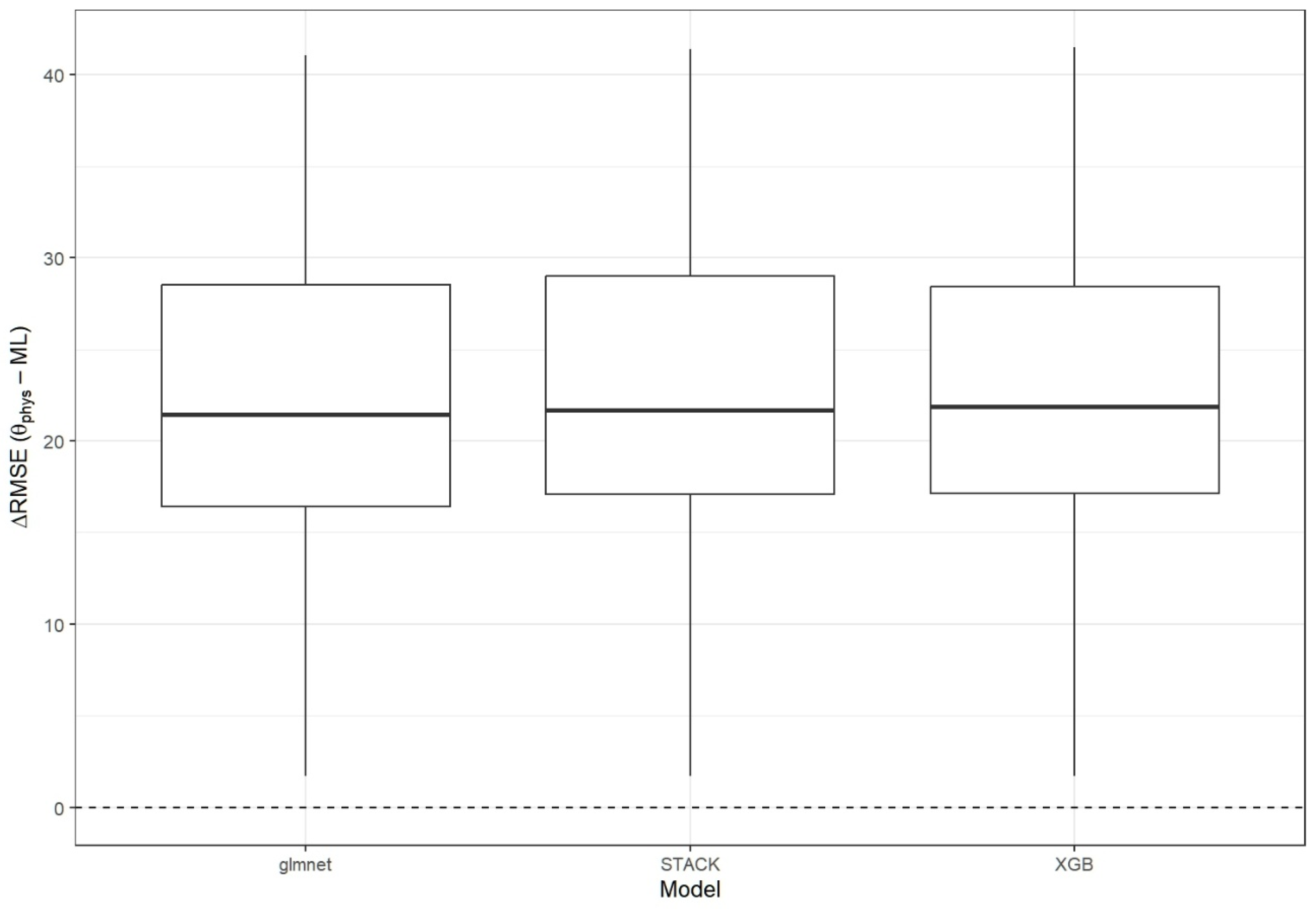
To quantify the contribution of the hybrid modeling approach, a physically based soil moisture estimate (${\widehat{\theta }}_{phys}$), derived from a radar scattering model, was used as a baseline reference. Model performance was compared against this physical benchmark using identical validation periods and spatial configurations. For each sensor, depth, orbit and temporal subset, ${\widehat{\theta }}_{phys}$ was evaluated against in situ observations using the same temporal grouping as the ML models. Performance metrics (RMSE, MAE and R²) were computed and directly compared with those obtained from the data-driven models (GLMNET, XGB and STACK). Performance gains were expressed as ΔRMSE, defined as the difference between the RMSE of ${\widehat{\theta }}_{phys}$ and that of each ML-based approach, ensuring a consistent and conservative assessment under the strict interannual validation context. This comparison was not intended to isolate the individual contribution of ${\widehat{\theta }}_{phys}$ within the machine learning models, but rather to assess the overall gain achieved by combining physical constraints with multi-source remote sensing and machine learning.

3. Results

3.1. Model Selection by Probe

The optimal model for each probe was selected using the weighted performance score described in the Section 2.9, considering only those models that met the generalization criteria (RMSE ≤ 5 and R² ≥ 0.5) and depths shallower than 0.35 m, representative of the active root zone. This selection strategy ensures that the chosen models exhibited not only good calibration performance but also robustness when applied to unseen data.

Table 3. Best models per probe, validation metrics, and years used for calibration and validation.

ProbeID	Depth (m)	Model	R2 Val	RMSE (% vol)	Bias (% vol)	Cal Year	Val Year
BT002990	0.25	GLMNET	0.758	1.127	−0.58	2023	2024
BT002994	0.15	GLMNET	0.669	1.034	−0.44	2023	2024
BT002996	0.35	RF	0.596	2.494	−1.33	2022	2023
CERRO_NADORCOTT	0.15	GLMNET	0.685	3.674	−2.54	2022	2023
CERRO_ORRI	0.15	GLMNET	0.709	3.467	2.37	2023	2024
Muela	0.35	SVR	0.690	0.345	−0.04	2024	2025
Salinas_S3	0.25	GLMNET	0.549	0.687	0.43	2023	2024

summarizes the results of the selected models per probe, including depth, validation metrics (R², RMSE, and bias), and the years used for calibration and validation. The results revealed a clear variability in algorithm performance depending on site-specific conditions. Regularized linear models (GLMNET) were selected for most probes, indicating that a parsimonious, physically informed linear structure was sufficient to capture soil moisture dynamics. In contrast, Random Forest and Support Vector Regression were preferred in a smaller number of cases, reflecting situations where nonlinear relationships or site-specific effects were more pronounced.

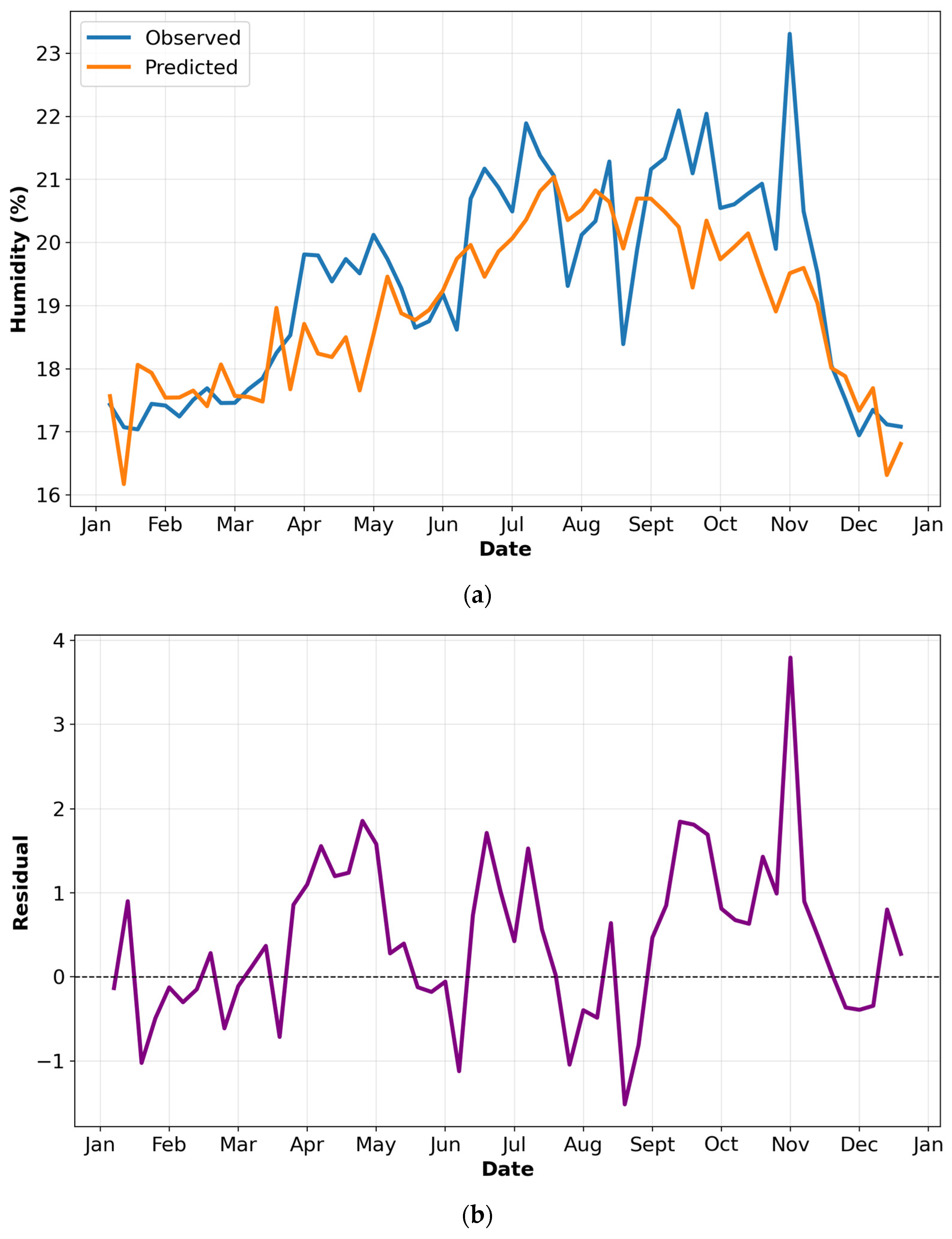
To illustrate model behavior under contrasting conditions, two representative probes were selected. Figure 3 shows results for probe BT002994 at 0.15 m depth, for which GLMNET achieved strong performance, with a high coefficient of determination (R² = 0.67), moderate error (RMSE ≈ 1.03% vol), and low bias. The predicted and observed time series during the validation year exhibited a high degree of temporal coherence, and residuals remained close to zero without evident systematic trends. This behavior indicated that the model successfully captured soil moisture dynamics in the surface layer.

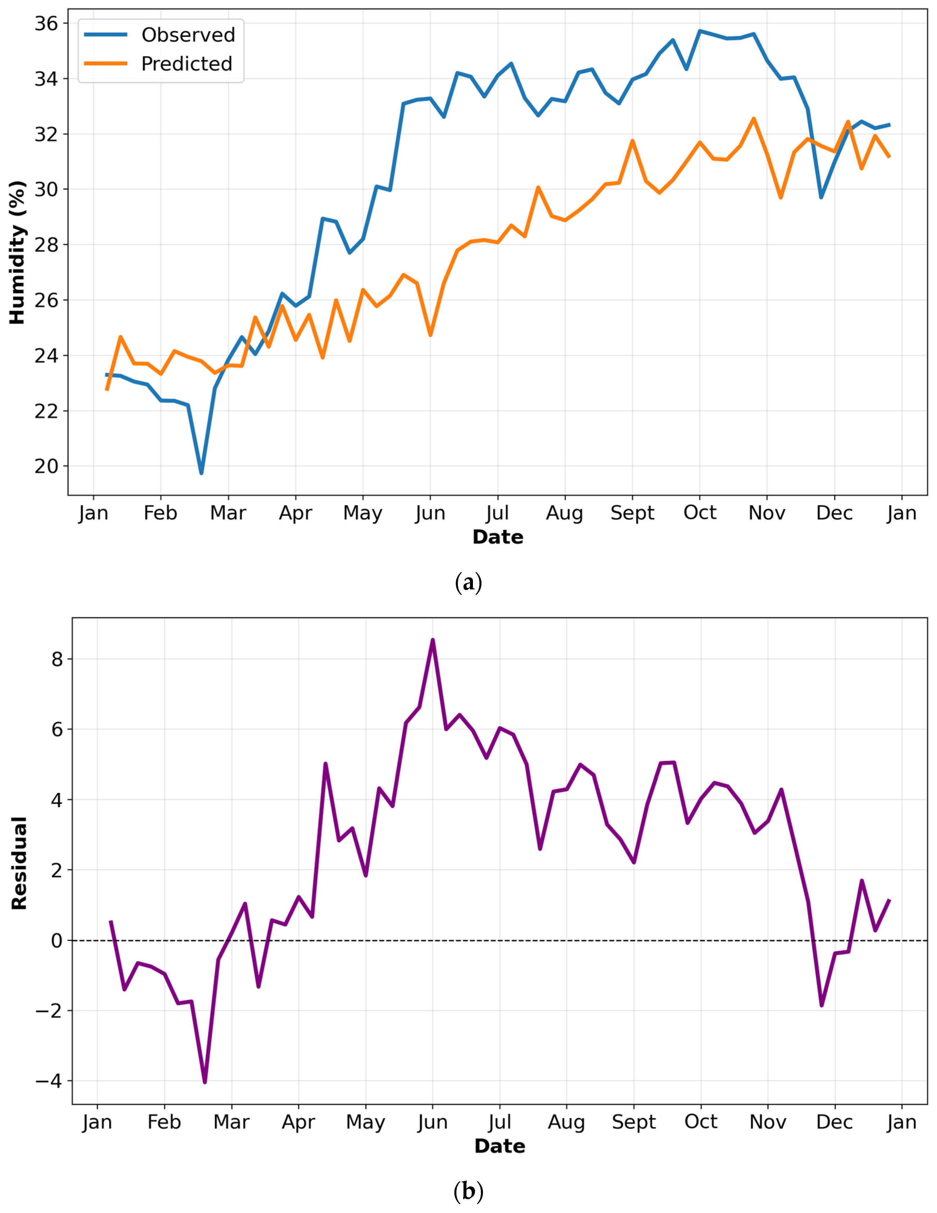
In contrast, Figure 4 corresponds to probe CERRO_NADORCOTT (0.15 m depth), also modeled with GLMNET but showing substantially lower performance. Although R² remained within acceptable limits, the higher RMSE (≈3.67% vol) and pronounced negative bias (−2.54% vol) indicated systematic underestimation. The temporal series revealed persistent deviations between predicted and observed values, suggesting local factors—such as soil heterogeneity or irrigation management—that were not fully captured by the available predictors.

3.2. Most Influential Variables by Probe

After selecting the best-performing model for each probe, the relative importance of predictor variables was analyzed. Variable importance scores were averaged across the two interannual validation folds and normalized to a 0–100 scale.

Table 4. Top 4 influential variables for each selected model by probe and relative importance.

Probe	Variable (Relative Importance)
BT002990	vsm4 (100), precip (43.4), NMDI2 (21.8), VV/VH (7.9)
BT002994	temp (85.8), vsm4 (74.3), precip (26.3)
BT002996	vsm4 (98.6), temp (87.9), vsm3 (79.0), vsm2 (77.2)
CERRO_NADORCOTT	vsm4 (100), tevap (60.4), vsm3 (51.4), temp (41.6)
CERRO_ORRI	vsm4 (97.5), temp (70.6), MNDWI (29)
Salinas_S3	MSI (100), vsm4 (93.2), ${\widehat{\theta }}_{phys}$ (78.1), temp (65.6)
BT002990	vsm4 (100), precip (43.4), NMDI2 (21.8), VV/VH (7.9)
BT002994	temp (85.8), vsm4 (74.3), precip (26.3)

reports, for each probe, the four most influential predictors and their relative contributions.

The results revealed substantial spatial variability in the dominant explanatory variables. ERA5-Land predictors, particularly deep-layer soil moisture (vsm4) and near-surface air temperature (temp), dominated most probes, reflecting the strong control exerted by large-scale hydrometeorological conditions on soil moisture dynamics in irrigated perennial systems.

In contrast, for specific locations such as Salinas_S3, optical indices (MSI) and the physically derived soil moisture estimate (${\widehat{\theta }}_{phys}$) emerged as key predictors. This highlighted the context-dependent added value of combining optical remote sensing information with physically based radar inversion, particularly under conditions of dense canopy cover or localized irrigation management.

3.3. Global Variable Importance

Beyond the probe-level analysis, a global ranking of predictor importance was obtained by aggregating normalized importance scores across all selected models and probes.

Table 5. Order of predictor variables by cumulative importance.

Variable	Cumulative Importance
vsm4	1812.93
Temp	879.11
Tevap	268.40
vsm3	184.38
MSI	173.28
NDMI	168.73
Precip	168.28
vsm1	166.80
MNDWI	150.17
NMDI2	144.98
NDVI	144.31
${\widehat{\theta }}_{phys}$	137.30
VV	136.53
NMDI	135.50
vsm2	125.00

presents the 15 most influential variables based on their cumulative importance.

The global ranking confirmed the dominant role of meteorological and soil state variables, particularly deep-layer soil moisture from ERA5-Land (vsm4) and air temperature (temp), as primary drivers of soil moisture variability. Among optical predictors, MSI and NDMI showed the strongest contributions, consistent with their sensitivity to vegetation water status.

SAR-derived variables, including VV backscatter, exhibited lower but non-negligible importance, becoming particularly relevant under conditions of limited optical data availability or dense canopy cover. Although the cumulative importance of the physically derived soil moisture estimate (${\widehat{\theta }}_{phys}$) did not rank among the most influential predictors, it was a key predictor for specific locations. Overall, these results demonstrated the complementary contribution of climatic, optical, SAR, and physical predictors.

3.4. Comparison with the Physical Baseline

Across all sites, depths, and acquisition geometries, the physically based baseline (${\widehat{\theta }}_{phys}$) exhibited substantially larger errors than the hybrid and data-driven machine learning approaches (including models using ${\widehat{\theta }}_{phys}$ as an auxiliary predictor). Under validation conditions, ${\widehat{\theta }}_{phys}$ showed RMSE values that were consistently higher than those obtained with machine learning models, while ML-based approaches typically reduced RMSE to values below 10% volumetric water content and often below 5% in the upper soil layers (0.05–0.35 m).

Relative to ${\widehat{\theta }}_{phys}$, the hybrid STACK model achieved systematic and substantial error reductions. Median ΔRMSE values under validation conditions ranged from approximately 15% to over 35%, with the largest gains observed in shallow and intermediate depths. Comparable improvements were obtained with XGBoost and GLMNET, although the STACK model exhibited the most consistent performance across probes and orbital configurations (Figure 5).

These performance gains were observed consistently across orchards, indicating that the improvement is not site- or geometry-specific but reflected a general enhancement provided by learning residual corrections over the physical baseline.

4. Discussion

4.1. Added Value of the Hybrid Physical–Machine Learning Methodology

The results clearly indicated that embedding physically based soil moisture estimates within machine learning models provided added value for orchard-scale soil moisture estimations in citrus orchards. While physics-only inversions reproduced the main temporal dynamics, their reduced accuracy under wet conditions and dense canopy cover reflected well-known limitations related to vegetation attenuation and surface roughness parameterization in perennial systems [7,8].

The hybrid approach alleviated these constraints by constraining the learning process within physically meaningful bounds, improving temporal consistency and robustness across varying soil moisture states and canopy conditions. This behavior was consistent with previous studies that advocated hybrid physical–data-driven approaches as an effective compromise between interpretability and predictive performance [5].

The comparison with the physical-only baseline highlighted the limitations of relying exclusively on simplified scattering models for orchard-scale soil moisture estimation in perennial crops. Although ${\widehat{\theta }}_{phys}$ captured first-order soil moisture dynamics, its large errors indicated that radar backscatter alone was insufficient to resolve the combined effects of canopy structure, roughness and irrigation-driven variability.

Rather than replacing physical modeling, the hybrid approach leveraged it as a physically meaningful reference state that constrained data-driven learning. The large and consistent ΔRMSE observed across sites and depths demonstrated that most of the predictive skill arose from learning nonlinear interactions between radar signals, vegetation indices and atmospheric drivers, rather than from the physical model alone. Importantly, these gains persisted under strict interannual validation, confirming that the improvement was not the result of temporal leakage or overfitting.

4.2. Interpretation of Algorithmic Performance

Tree-based ensemble models generally outperformed linear and kernel-based approaches, reflecting their ability to capture nonlinear interactions among radar backscatter, vegetation indices, and agroclimatic drivers. The achieved performance range (R² ≈ 0.55–0.76) was consistent with values reported in the literature for Sentinel-1 and Sentinel-2-based soil moisture estimation [4,5] over agricultural areas and reflected the combined influence of irrigation practices, soil properties, canopy development, and atmospheric demand.

The variable importance analysis emphasized the complementary contribution of physical, climatic, and remote sensing predictors. Physically informed variables, such as the inverted soil moisture proxy (${\widehat{\theta }}_{phys}$) and Sentinel-1 backscatter metrics, encoded scattering mechanisms that were not directly accessible through purely statistical predictors.

ERA5-Land variables, particularly soil moisture in deeper layers and air temperature, played a dominant role in many orchards, stabilizing predictions between satellite acquisitions and capturing the hydrometeorological memory of the soil–plant–atmosphere system [13,14]. Sentinel-2 vegetation indices provided additional explanatory power during periods of canopy development and transition, reinforcing the value of combining optical and radar information.

The use of a strict interannual validation strategy provided confidence in the operational relevance of the proposed approach by explicitly limiting temporal information leakage. The stability of model performance across contrasting years indicated that the proposed hybrid approach was not overly dependent on year-specific patterns and could adapt to varying irrigation schedules and meteorological conditions.

These results support the potential operational deployment of the hybrid framework for orchard-scale soil moisture monitoring in citrus systems, particularly in contexts where continuous in situ measurements are limited.

4.3. Limitations and Perspectives for Improvement

This study has several limitations. First, aggregating Sentinel-1/2 observations to the orchard level can smooth within-orchard spatial variability and introduce scale mismatch relative to point-scale FDR measurements. Second, the causal nearest-past matching used to align optical indices with probe dates may introduce temporal lag or bias under rapidly changing canopy conditions or soil moisture states. Third, imputing missing values by forward propagation assumes short-term persistence that may break down following irrigation events or intense rainfall. Fourth, although ERA5-Land variables provide temporally coherent context, their coarse spatial resolution may limit representativeness at orchard scale.

Physically based inversions remain sensitive to surface roughness and vegetation structure assumptions, while FDR sensors may not fully capture sub-parcel heterogeneity. In addition, direct transferability to other sites should be considered with caution, as calibration of physical parameters and reliance on site-specific sensors introduce a degree of local dependency.

Future work should incorporate robust, multiscale gap-filling strategies and management variables (e.g., irrigation and fertigation logs) to better represent human-driven dynamics. Priority should also be given to dynamic calibration of vegetation attenuation parameters, extension across multi-site and multi-year datasets, and systematic hyperparameter optimization alongside evaluation of additional hybrid formulations. These developments are expected to improve robustness, generalization, and applicability across perennial cropping systems.

5. Conclusions

This study demonstrated the potential of the proposed hybrid physical–machine learning approach for orchard-scale soil moisture monitoring in irrigated citrus orchards using operational data sources. By integrating Sentinel-1 and Sentinel-2 observations, ERA5-Land agroclimatic variables, and in situ FDR measurements within a physics-informed machine learning design, the proposed approach delivers robust daily soil moisture estimates under strict interannual validation.

The results showed that physically meaningful predictors improved model stability and generalization, while multi-source data fusion captured the complex controls governing soil moisture dynamics in perennial cropping systems. Benchmarking against a physical-only baseline demonstrates that the hybrid methodology provided a clear and consistent improvement over simplified radar-based soil moisture retrievals, with substantial reductions in prediction error across sites and depths.

Although challenges remain under extreme conditions and dense canopy cover, the proposed methodology provides a solid and scalable basis for soil moisture monitoring in Mediterranean citrus orchards and related perennial crops, supporting the development of advanced irrigation decision-support tools.

This approach contributes to bridging the gap between remote sensing theory and operational irrigation management in perennial Mediterranean systems. By leveraging open and operational satellite data streams, the proposed methodology can inform decision support tools for farmers and water authorities, contributing to sustainable irrigation, risk mitigation under climate variability, and ultimately to food security goals in perennial cropping systems.