Interpretable Deep Learning for Varroa Mite Detection: Integrating Deblurring, Morphology-Preserving Preprocessing, and Explainability Analysis

Abstract

Varroa destructor is the most devastating ectoparasite of Apis mellifera, and early detection is critical for colony survival. This study systematically investigated how image preprocessing, model architecture, and feature map resolution jointly affect classification accuracy and Grad-CAM++ explainability in deep-learning-based Varroa detection. From comb-surface images of 20 A. mellifera colonies, 3400 region-of-interest images were processed through 12 preprocessing pipelines combining deblurring, histogram normalization, morphology-preserving resizing, and non-morphological resizing. Nineteen CNN architectures, including VarroaNet — a custom lightweight model with configurable channel attention — were screened across all pipelines, and the top six further evaluated at four feature-map resolutions (7 × 7 to 56 × 56); the two stages together comprised 1,548 classification training runs across 516 configurations. Resizing consistently improved classification accuracy, whereas histogram normalization degraded it. VarroaNet (r = 8) achieved the highest mean accuracy across configurations (97.28%) with the lowest cross-configuration variability (CV = 1.47%). The 28 × 28 resolution was jointly optimal for classification and localization at minimal computational overhead, whereas 56 × 56 degraded performance. Notably, classification accuracy and localization quality did not always coincide—the highest-accuracy configuration (ShuffleNet-V2-x1.0 at 14 × 14, 97.34%) achieved an IoU@30 of only 0.160, underscoring the need for explicit localization evaluation. Morphology-preserving resizing achieved higher localization efficiency with zero morphological distortion. The recommended configuration—VarroaNet (r = 8) at 28 × 28 with deblurred MR preprocessing—achieved the highest localization performance (Pointing Game = 0.927), indicating correct attention to the mite region in 92.7% of infested test images.

1. Introduction

The beekeeping industry is a vital sector, crucial not only for producing honey, pollen, and beeswax but also for pollinating agricultural crops [1]. However, it faces significant threats, among which the parasitic mite Varroa destructor is particularly damaging, disrupting the normal development of adult bees, pupae, and larvae, and contributing substantially to colony collapse and declining bee populations [2,3,4,5,6]. Current diagnostic methods for Varroa mite infestation include visual inspection, the sugar roll method, and bottom board examinations. These methods are subject to the inherent limitation of requiring direct counting of Varroa mites after their acquisition from the beehive. Furthermore, because the entire procedure is executed manually, it is susceptible to human-induced variability. Specifically, visual identification is challenging, owing to the small size (1.6 × 1.1 mm) of the mite and its reddish-brown protective coloration, which blends in with the bees [7,8]. Furthermore, the difficulty of real-time monitoring often leads to a reliance on scheduled acaricide applications for control, which can promote acaricide resistance in Varroa populations and lead to chemical residues in hive products [9]. Although synthetic acaricides are effective against mites, their adverse effects on honey bees have made organic treatments the preferred alternative. This trade-off highlights the importance of early, targeted detection strategies that minimize the need for broad chemical interventions [10]. Therefore, developing rapid, early diagnostic technologies is crucial for controlling Varroa mites at the initial stage of infestation, thereby minimizing acaricide use.

Recently, research in the beekeeping industry has increasingly focused on the digitalization of hive data and the introduction of automation technologies. For instance, studies have explored the use of internet-of-things-based systems for real-time collection and analysis of apicultural data [11]. Among these advancements, the development of technologies for bee health monitoring and disease diagnosis using computer vision and artificial intelligence (AI) has gained significant attention. In particular, deep-learning-based identification of Varroa destructor has gained prominence, with proposed techniques primarily utilizing convolutional neural network (CNN) and You Only Look Once (YOLO) models. While some studies have used CNN architectures to classify general beekeeping objects, such as eggs, larvae, and pupae [12,13], others have focused specifically on Varroa mite identification. For example, one study applying a CNN-based model reported an accuracy of 89.5% on original images, which improved to 99.99% after a 100-fold data augmentation [14]. In the domain of object detection, an F1-score of 97.01% has been achieved by combining a YOLO model with a background removal network [15]; another YOLO-based model demonstrated a 95% F1-score for simultaneously identifying bees, pollen, and Varroa mites within hives [16]. Furthermore, a study utilizing a CNN with a feature pyramid network (FPN) reported a mean average precision (mAP) of 90.73% for recognizing mites on bottom board inspection sheets [17]. More recent work has applied AI-enhanced image preprocessing to small-object mite detection [18]. In parallel, lightweight architectures and explainable AI for plant and pest detection have been comprehensively reviewed [19,20]. However, previous studies have several key limitations. Although CNN-based models have demonstrated high accuracy, they often lack validation to ensure that the predictions made by the model are based on the actual morphological features of the mites rather than on confounding background cues. Furthermore, many models are trained on image data collected against simple, uniform backgrounds, which may limit their applicability and robustness in complex, real-world beekeeping environments.

To enhance the real-world applicability of these AI models, the specific image regions that guide their predictions need to be evaluated. This has led to research into algorithms that analyze the regions where a model concentrates its computational weight, such as on the object, its boundaries, or the background. In particular, techniques such as class activation mapping (CAM) and gradient-weighted class activation mapping (Grad-CAM) serve as powerful tools for visualizing the key regions that a neural network focuses on to detect an object during inference [21,22]. Such methods improve a model’s explainability, enabling verification that decisions are based on relevant patterns. For instance, a study on grape leaf disease used Grad-CAM to confirm that a CNN model was indeed focusing on lesion areas to make its diagnosis [23]. Therefore, weight visualization algorithms enable validation that an AI model focuses on the actual object of interest rather than spurious background information, which is a crucial step in enhancing its practical utility and reliability [19]. However, while such qualitative observations offer initial insights, they often lack the empirical rigor required for objective benchmarking. The present study addresses this limitation by shifting the focus toward a systematic quantitative analysis, thereby providing a reproducible framework for evaluating model explainability and classification fidelity.

The necessity for rigorous validation is underscored by the practical challenges of Varroa mite management, which extend far beyond simple recognition accuracy. The short life cycle of Varroa mites means that suboptimal control strategies can quickly lead to acaricide misuse and the development of resistance [24,25]. Critically, misidentifications by an AI model can have severe consequences. False positives may lead to unnecessary chemical treatments that harm a colony’s health, while false negatives can result in delayed responses that risk the loss of the entire colony. This context emphasizes the necessity of developing highly reliable AI models for accurate Varroa mite identification and of rigorously validating their practical applicability, for which both advanced AI architectures and interpretability techniques like Grad-CAM are essential.

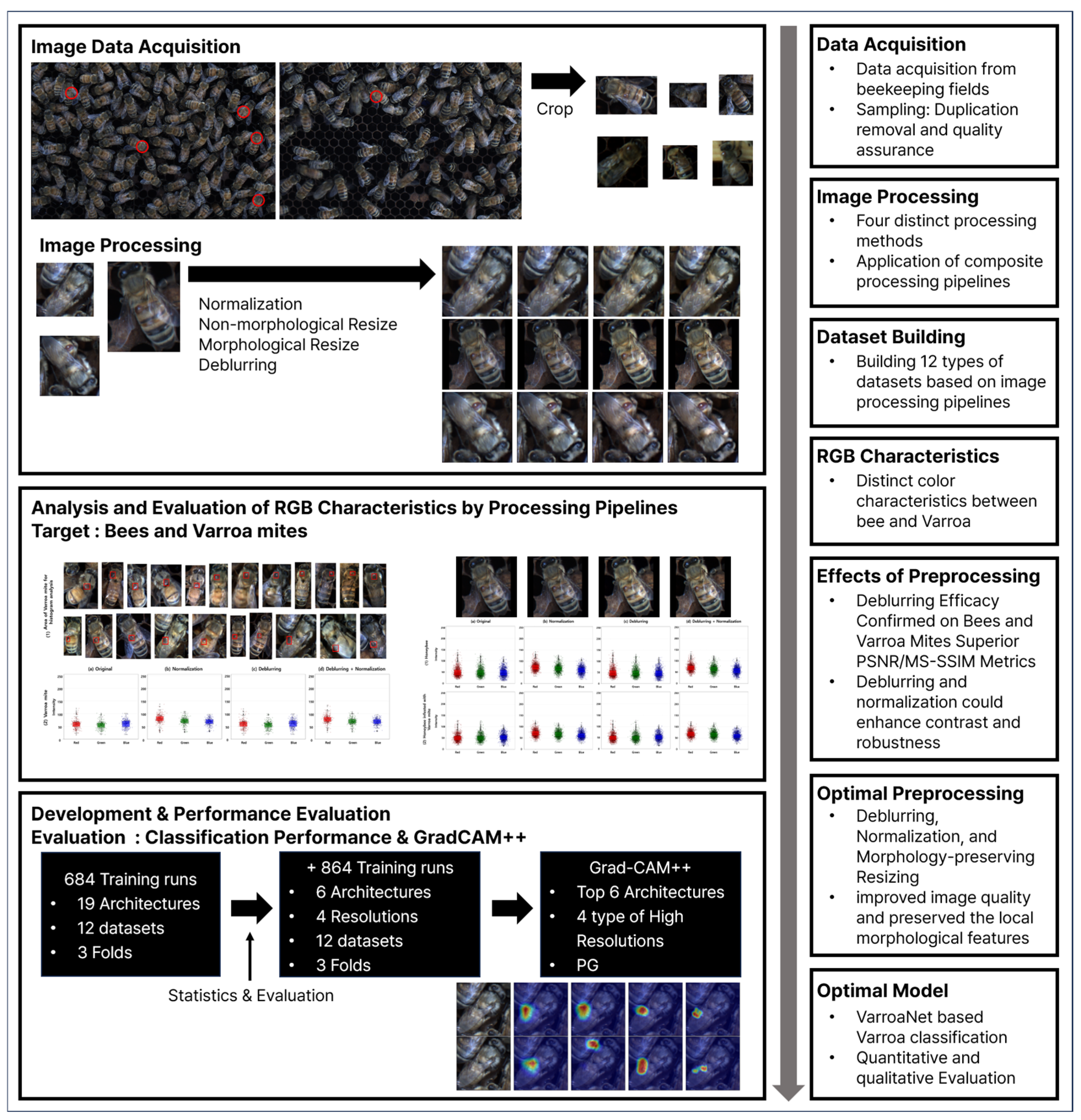
Images from beekeeping environments are inherently challenging, as they involve fast-moving living organisms whose sudden movements can degrade image quality, even under fixed measurement setups. In agriculture, deblurring algorithms have been successfully used to correct for such motion-induced degradation. Deep-learning-based deblurring techniques, in particular, have demonstrated superior restoration performance over traditional methods in precision agriculture, with studies successfully applying algorithms such as the scale recurrent network, Deep-Deblur, and DeblurGAN-v2 to improve fruit detection in grape imagery [26,27]. In the beekeeping domain, the motion blur from the rapid movements of bees, combined with the small size of the target mites, renders accurate identification particularly difficult even in otherwise clear images. However, research applying deblurring technologies to address this specific issue remains limited. This study aimed to improve the quality of bee and mite imagery through the application of deblurring. Therefore, this study aimed to develop and validate CNN-based models capable of distinguishing between normal bees and those infested with Varroa mites, using bee comb images acquired in real beekeeping environments. Twelve preprocessing pipelines were constructed under a 2 × 2 × 3 factorial design combining deblurring, histogram normalization, and resizing (none, non-morphological resize, or morphology-preserving resize), enabling the marginal and interaction effects of each factor to be isolated. Nineteen architectures of varying parameter scale and structural design—including CNNs (ResNet, MobileNetV2/V3, EfficientNetB0, ShuffleNetV2, RegNetY-400MF), a Transformer-based model (Swin Transformer), and a custom lightweight network with configurable channel attention, VarroaNet (r = 4, 8, 16)—were first screened across all twelve pipelines, and the top-performing entries were then re-evaluated across four feature map resolutions (7 × 7 to 56 × 56) to examine how spatial granularity interacts with architecture and preprocessing choice. Grad-CAM++ was further applied to assess whether classification-optimal configurations also attended to the actual mite region. Across all stages, a total of 1548 training runs were systematically compared to identify the optimal combination of preprocessing, architecture, resolution, and attention strength for reliable and interpretable Varroa mite identification. An overview of the proposed framework is shown in Figure 1.

2. Materials and Methods

2.1. Image Acquisition and Dataset Construction

Images of normal bees and bees infested with Varroa mites were collected to construct a dataset for deep learning model development. Image data were collected at apiaries in Chuncheon, Gangwon-do, and at the National Institute of Agricultural Sciences in Wanju-gun, Jeollabuk-do, Republic of Korea, encompassing a total of 20 hives. The bee species used in this study was the Western honey bee (Apis mellifera).

Images were acquired using a Blackfly S GigE camera (BlackflySGigE, FLIR, Wilsonville, OR, USA) at a spatial resolution of 2048 × 1536 pixels and a working distance of approximately 300 mm. Image acquisition was performed in a shaded outdoor environment to maintain relatively consistent lighting conditions and to avoid specular reflections on the comb surface.

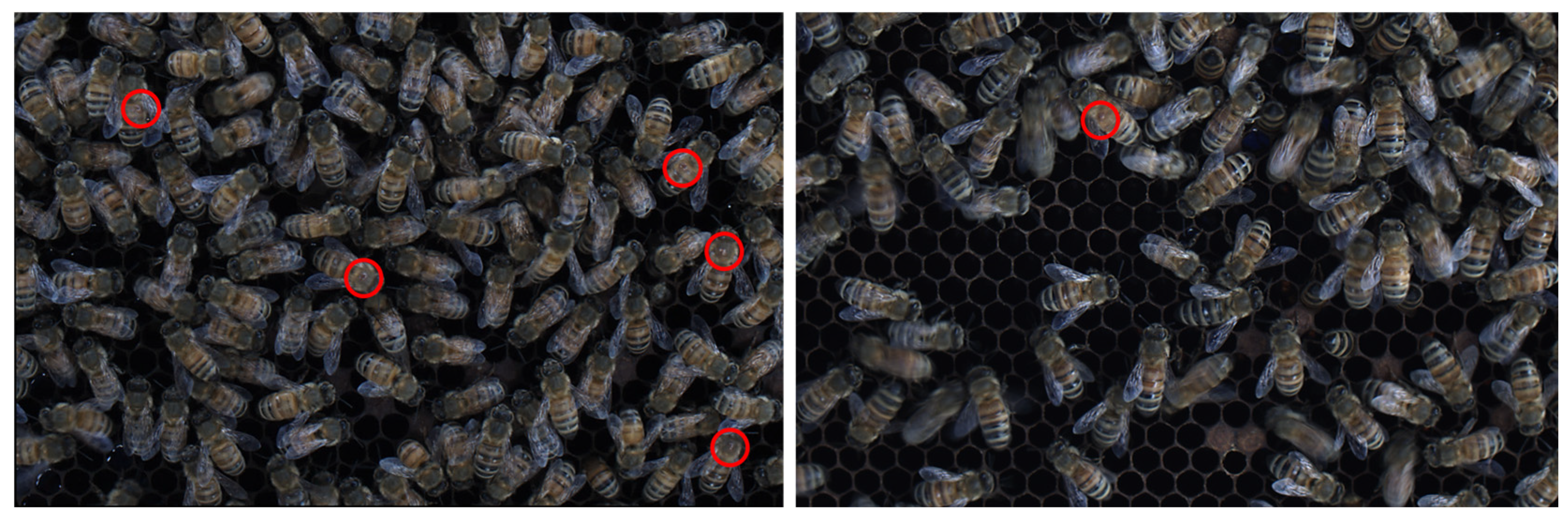
In a typical apiary environment, the population of Varroa mites is significantly smaller than that of bees. To construct a balanced dataset essential for training a robust classification model, frames containing mite-infested bees were selectively sampled from the total footage acquired. To enhance model generalization and prevent temporal correlations, images from consecutive frames were discarded. The dataset was also curated by excluding severely blurred or out-of-focus images that did not permit reliable visual inspection. Although bee posture and angle were disregarded, only images in which both the bees and attached mites were clearly visible on the comb surface were retained in the final dataset to ensure relevance to real-world conditions (Figure 2). From these curated images, regions of interest (ROIs) were later extracted as described in Section 2.2, resulting in a total of 3400 bee ROI images (1700 normal and 1700 Varroa-infested).

2.2. ROI Generation and Preprocessing Design

For deep-learning-based model training, ROIs corresponding to normal bees and Varroa-infested bees were designated and extracted using the OpenCV library in Python (version 3.11). From the curated images, a total of 3400 ROI images were obtained, comprising 1700 normal and 1700 Varroa-infested bee images. Although all images were acquired at an identical shooting distance, ROI image sizes varied due to differences in bee posture and angle (Figure 3). Additionally, images captured in actual beekeeping environments showed diverse image quality caused by sunlight changes, weather, and individual hive characteristics. Image preprocessing was therefore applied to mitigate these effects and render the images suitable for deep learning computation.

2.2.1. Image Resizing, Normalization, and Deblurring Methods

All extracted ROI images were resized to a uniform dimension of 224 × 224 pixels to meet the input requirements of the deep learning models. Two resizing methods were defined in this study: morphology-preserving resizing and non-morphology-preserving resizing. Morphology-preserving resizing involved scaling each image while maintaining its original aspect ratio until one dimension reached 224 pixels, after which padding was applied to the other dimension to fill the remaining space. Histogram normalization was implemented as per-channel min–max linear stretching, in which each RGB channel was independently rescaled for each image to fully occupy the [0, 255] dynamic range, thereby standardizing exposure across images while preserving the within-channel intensity ordering. In contrast, non-morphology-preserving resizing directly stretched or compressed the image to fit the 224 × 224 frame, without preserving the original proportions. Numerical instabilities during preprocessing, such as arithmetic overflow from enhancement algorithms, division-by-zero errors in histogram-based adjustments, and information loss from interpolation artifacts during resizing operations, were mitigated by consistently clipping pixel intensities to the range of 0–255 following each computational step.

Several deblurring algorithms were considered for motion blur correction, including the Wiener filter, deep-learning-based methods (MPRNet, DMPHN), and generative adversarial network (GAN)-based approaches (DeblurGAN, DualGAN). Among traditional methods, the Wiener filter optimizes the signal-to-noise ratio and provides effective linear correction for simple image structures [28]. However, this approach was found to be inadequate for beekeeping imagery containing diverse features and relatively small objects such as Varroa mites. Deep-learning-based approaches employ distinct architectural strategies. MPRNet utilizes a progressive encoder–decoder architecture that efficiently leverages stage-wise features [29]. DMPHN processes images through patch-based division for localized blur removal [30]; however, this approach is unsuitable for small-sized images due to computational limitations. In contrast, GAN-based methods (DeblurGAN, DualGAN) generate reconstructed sharp images rather than performing direct correction [31,32]. This generative approach may introduce artifacts that deviate from original measured data, potentially compromising field applicability for precise imaging requirements. Therefore, MPRNet was selected for its capability to process complete image data without dimensional constraints while maintaining fidelity to original measurements.

2.2.2. Dataset Configuration

To systematically evaluate the individual and combined effects of preprocessing techniques, twelve distinct datasets were constructed by combining two resizing methods—morphology-preserving resizing (MR) and non-morphological resizing (NR)—with histogram normalization and deblurring processes. This design enabled the assessment of the contribution of each preprocessing method and their combined effects (

Table 1. Image processing methods applied to each dataset.

Dataset	Image Processing Methods
Dataset 1	Original
Dataset 2	Normalization
Dataset 3	Non-morphological resize (224 × 224)
Dataset 4	Morphology-preserving resize (224 × 224)
Dataset 5	Normalization, non-morphological resize (224 × 224)
Dataset 6	Normalization, morphology-preserving resize (224 × 224)
Dataset 7	Deblurring
Dataset 8	Deblurring, normalization
Dataset 9	Deblurring, non-morphological resize (224 × 224)
Dataset 10	Deblurring, morphology-preserving resize (224 × 224)
Dataset 11	Deblurring, normalization, non-morphological resize (224 × 224)
Dataset 12	Deblurring, normalization, morphology-preserving resize (224 × 224)

). For the binary classification task, images were labeled as “1” for normal bees and “0” for Varroa-infested bees. The 3400 images were used for model development under the cross-validation and data-partitioning protocol detailed in Section 2.6, with stratified sampling applied throughout to preserve class balance between the two classes.

2.3. Image Quality Assessment Methods

The effects of deblurring and histogram normalization on image quality were evaluated using two commonly employed full-reference metrics: peak signal-to-noise ratio (PSNR) and multi-scale structural similarity index measure (MS-SSIM) [33,34]. Additionally, changes in intensity distribution by image processing were visualized through histograms to qualitatively assess the effects of normalization.

The PSNR quantifies the error between processed and original images on a logarithmic scale, calculated according to Equation (1). MAX represents the maximum possible pixel value (255 for 8 bit images), and MSE denotes the mean squared error between original and deblurred images. The variables m and n correspond to the vertical and horizontal pixel dimensions, respectively, where I(i, j) and K(i, j) represent pixel values in the original and deblurred images, respectively. PSNR values are expressed in decibels (dB), with higher values indicating superior restoration fidelity to the original image.

$$PSNR=10·lo{g}_{10}(MA{X}^2/MSE)$$

(1)

$$MSE=(1/(m\times n)){\displaystyle {\sum }_{i=0}^{m-1}}{\displaystyle {\sum }_{j=0}^{n-1}}[I(i,j)-K(i,j){]}^2$$

The MS-SSIM is a multi-scale extension of the structural similarity index that was developed to overcome the limitations of single-scale SSIM analysis [34]. Reflecting characteristics of the human visual system, which perceives images at various resolutions, the MS-SSIM evaluates structural similarity at five different scales. Images are iteratively downsampled at each scale to enable hierarchical analysis from fine details to overall structure. Calculated as shown in Equation (2), it combines luminance (l), contrast (c), and structure (s) components at each scale through weighted products. M represents the number of scales (=5), l_m(x, y) is the luminance comparison function at the highest scale, and c_j(x, y) and s_j(x, y) are, respectively, contrast and structure comparison functions at scale j. The per-scale exponents were assigned according to the weighting scheme proposed in a previous study, using the five-scale weight vector [0.0448, 0.2856, 0.3001, 0.2363, 0.1333] for scales j = 1–5, respectively [34]. These specific weights were experimentally optimized to mimic the varying sensitivity of the human visual system (HVS) to different spatial frequency bands, assigning the highest emphasis to intermediate scales, which aligns with the commonly accepted best practice for general image quality assessment.

$$\mathrm{M}\mathrm{S}\text{-}\mathrm{S}\mathrm{S}\mathrm{I}\mathrm{M}\left(x,y\right)={\left[l_M\left(x,y\right)\right]}^{{\alpha }_M}\hspace{0.17em}{\displaystyle {\prod }_{j=1}^M}{\left[c_j\left(x,y\right)\right]}^{{\beta }_j}{\left[s_j\left(x,y\right)\right]}^{{\gamma }_j}$$

(2)

$$l\left(x,y\right)={\displaystyle \frac{2{\mu }_x{\mu }_y+C_1}{{{\mu }_x}^2+{{\mu }_y}^2+C_1}}$$

$$c\left(x,y\right)={\displaystyle \frac{2{\sigma }_x{\sigma }_y+C_2}{{{\sigma }_x}^2+{{\sigma }_y}^2+C_2}}$$

$$s\left(x,y\right)={\displaystyle \frac{{\sigma }_{xy}+C_3}{{\sigma }_x{\sigma }_y+C_3}}$$

Differences in the PSNR and MS-SSIM between normal and mite-infested bee images were assessed using Welch’s t-test, which accommodates potentially unequal variances between the two independent groups.

Image quality grade criteria were defined based on prior research benchmarks. Previous studies have reported PSNRs ranging from 26.10 to 32.74 dB and MS-SSIM values between 0.7076 and 0.9066 for the general BSD100 dataset. For the more complex Urban100 dataset, maximum values of 35.09 dB and 0.9505 were recorded [35,36,37]. Based on these image quality research results, the image quality evaluation criteria were established, as shown in

Table 2. Image quality assessment criteria based on PSNR and MS-SSIM metrics.

	PSNR	SSIM
Normal	<26	<0.70
Good	26–30	0.70–0.85
Very Good	30–35	0.85–0.95
Excellent	>35	>0.95

.

2.4. Candidate Architectures and the VarroaNet Design

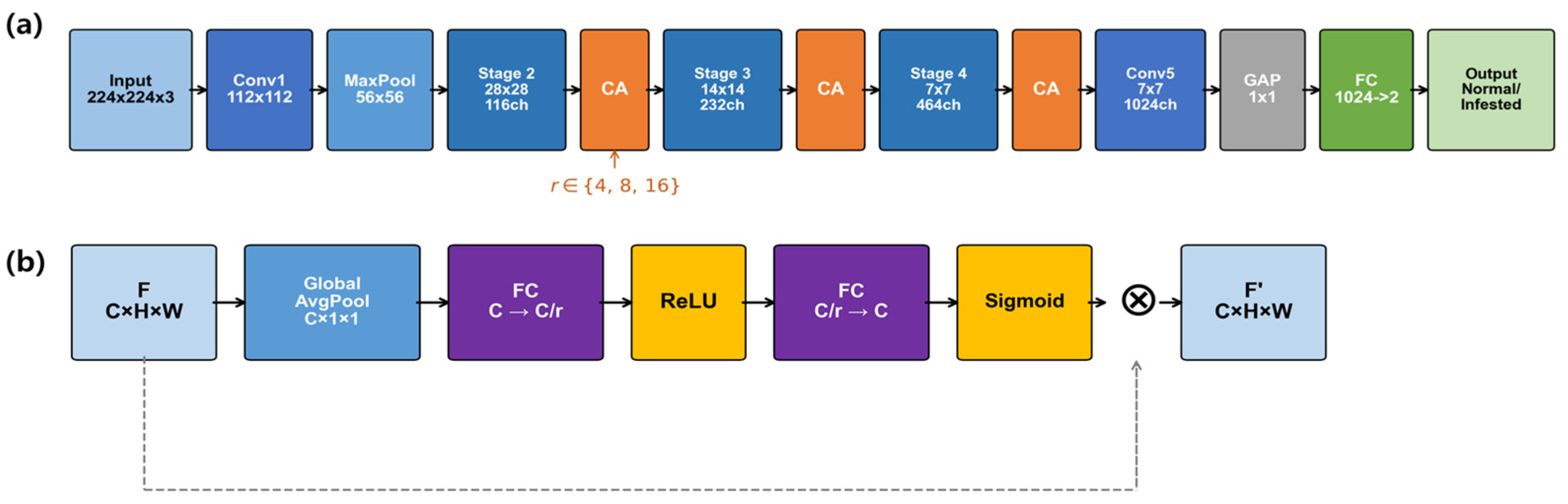
The VarroaNet architecture was introduced as a ShuffleNet-V2-derived variant, specifically configured to evaluate the synergy between channel attention intensity and spatial resolution within a constrained parameter budget (Figure 4). The model augments the ShuffleNet-V2 backbone with squeeze-and-excitation (SE) modules and a dedicated classification head, and the SE reduction ratio (r ∈ {4, 8, 16}) is treated as the sole varying factor. This design isolates the effect of channel-recalibration intensity on classification accuracy and Grad-CAM++ localization fidelity, while keeping all other architectural components—depth, width, channel-shuffle topology, and pretrained-weight initialization—identical across the three variants. The implementation is publicly available at https://github.com/2nugu/Varroanet-high-res-2D-CNN- (accessed on 15 June 2026).

The main characteristics of each architecture are summarized as follows. AlexNet and VGG11 were selected as fundamental deep learning structures that extract features and learn using matrix multiplication [38,39]. VGG11_bn improves training stability by adding batch normalization to the VGG11 structure. SqueezeNet was selected for its fire module architecture with parameter optimization using 1 × 1 convolutions [40]. GoogLeNet was employed for its inception modules that combine Hebbian principles and multi-scale processing to optimize computational cost and training efficiency [41]. The ResNet architecture was utilized for its residual blocks with skip connections to solve the gradient vanishing problem, with ResNet18 and ResNet50 selected based on parameter scale [42]. DenseNet121 was chosen for its ability to maximize feature reuse through dense block architecture, improving computational efficiency [43]. MobileNet and ShuffleNet were selected for their computational efficiency—the former employing depthwise separable convolution [44] and the latter channel shuffle operations [45]. EfficientNet was employed for its compound scaling methods to optimize the balance between model size and performance [46]. MNASNet optimizes models through a reinforcement learning-based neural architecture search [47]. RegNet improves the balance between computational efficiency and accuracy by regularizing structural elements using design space approaches [48]. Finally, Swin Transformer-S improves computational efficiency and performance through multi-head self-attention, shifted window-based Swin transformer blocks, and hierarchical feature maps, setting it apart from conventional Vision Transformer structures [49].

Table 3. Architectural specifications of the 19 candidate convolutional neural networks evaluated.

Models	Parameters (M)	Base Feature Map Resolutions	Attention
ResNet-50	23.5	7 × 7	None
ResNet-18	11.2	7 × 7	None
DenseNet-121	7.0	7 × 7	None
EfficientNet-B0	4.0	7 × 7	Built-in SE (r = 4)
MobileNetV2	2.2	7 × 7	None
MobileNetV3-Small	1.5	7 × 7	Built-in SE (r = 4)
ShuffleNet-V2-x1.0	1.3	7 × 7	None
ShuffleNet-V2-x0.5	0.3	7 × 7	None
GoogLeNet	5.6	7 × 7	None
RegNet-Y-400MF	3.9	7 × 7	None
MNASNet-1.0	3.1	7 × 7	None
SqueezeNet-1.0	0.7	13 × 13	None
AlexNet	57.0	6 × 6	None
VGG-11	128.8	7 × 7	None
VGG-11-BN	128.8	7 × 7	None
Swin-S	48.8	7 × 7	Window Attention
VarroaNet (r = 4)	1.4	7 × 7	Custom SE
VarroaNet (r = 8)	1.3	7 × 7	Custom SE
VarroaNet (r = 16)	1.3	7 × 7	Custom SE

summarizes the number of parameters for each architecture and the corresponding feature map resolution for XAI analysis.

The base feature map resolution inherent in many lightweight architectures was identified as a potential constraint that could impede the distinction of fine-grained morphological features of Varroa mites, especially considering that these targets typically occupy only a minimal portion of the total image area. To address this anticipated limitation in spatial granularity, a uniform stride modification strategy was applied to the selected architectures. This approach, informed by established principles for preserving spatial resolution without the introduction of additional parameters [50] and the management of multi-scale representations [51], allowed the feature map dimensions to be systematically expanded across four distinct levels: 7 × 7, 14 × 14, 28 × 28, and 56 × 56. By employing this balanced factorial design, the specific effects of spatial resolution were successfully isolated from other architectural confounding factors, such as network depth and channel capacity. This design was intended to facilitate a direct quantification of how resolution affects both diagnostic classification accuracy and Grad-CAM++ localization precision, thereby establishing a rigorous analytical framework to evaluate the trade-offs between model performance and interpretability.

2.5. Model Training Configuration and Implementation Environment

To ensure robust evaluation and avoid performance estimates that depend on a particular data partition, classification performance was assessed using 3-fold stratified cross-validation (random_state = 42) on the complete dataset of 3400 images. In each iteration, two folds were used for training and the remaining fold for evaluation, and the reported results correspond to the mean and standard deviation across the three folds. In contrast, for the Grad-CAM++ interpretability analysis, a model was trained on a single fixed 70%/20%/10% split, and the activation maps were generated on the held-out 10% test set (Section 2.6).

The model was optimized using CrossEntropyLoss and the AdamW(lr = 0.01, weight_decay = 0.01) optimizer, decoupling weight decay from the gradient updates to enhance generalization performance [52]. A ReduceLROnPlateau scheduler (factor = 0.5, patience = 3) was applied to adapt the learning rate during training. Models were trained for up to 500 epochs with early stopping to mitigate overfitting. Training was terminated when the monitored loss failed to improve by more than 0.0005 (min_delta) for 12 consecutive epochs (patience = 12); the monitored loss was computed on the held-out fold during cross-validation and on the validation set in the fixed-split experiments. The batch size was set to 32 for the 7 × 7, 14 × 14, and 28 × 28 input resolutions and to 8 for the 56 × 56 resolution.

The dataset constructed in this study contains only images measured on bee combs, resulting in limited background information and potential overfitting risks due to insufficient data diversity. Transfer learning was applied to overcome these data limitations and improve model generalization performance. Models were initialized using pretrained weights from the ImageNet-1k dataset. Transfer learning utilizes these weights for training on new datasets, offering the advantage of achieving high performance based on object information learned from other image data [53,54]. The model development environment was constructed using Python and PyTorch, with hardware and software specifications shown in

Table 4. Hardware and software environments for deep learning model development.

Parameters	Specification
CPU	AMD Ryzen 3960X 3.80 GHz
GPU	Nvidia RTX 3090 (CUDA 12.6)
RAM	256 GB
Programming language	Python 3.11
Deep learning library	Pytorch-gpu (CUDA 12.6)

.

2.6. Experimental Design and Evaluation Framework

A total of 19 CNN architectures were evaluated across 12 preprocessing datasets using 3-fold stratified cross-validation (K = 3, random_state = 42), totaling 684 independent runs. The primary objectives were architecture ranking, statistical sensitivity analysis of preprocessing factors, and an ablation study on the VarroaNet SE reduction ratio (r = 4, 8, 16). Statistical significance was assessed using the Wilcoxon signed-rank test and Cohen’s d effect size, while Kendall’s coefficient of concordance (W) evaluated model ranking consistency across pipelines. Models with a grand mean accuracy below 80% were classified as convergence failures and excluded from the preprocessing sensitivity analysis.

Following the initial screening, the six selected architectures were further evaluated across four feature map resolutions (7 × 7, 14 × 14, 28 × 28, and 56 × 56) and the 12 preprocessing datasets, yielding 288 architecture–resolution–preprocessing configurations. Classification performance was assessed using 3-fold stratified cross-validation, resulting in 864 training runs (288 configurations × 3 folds). This procedure enabled all images to contribute to both training and evaluation while reducing dependence on any particular dataset partition. Equivalence among the VarroaNet variants (r = 4, 8, and 16) was assessed using the two one-sided test (TOST) procedure with equivalence margins of δ = ±0.5 pp and ±1.0 pp.

Grad-CAM++ analysis was performed using a separate fixed-split protocol. Localization metrics require that saliency maps be generated on images excluded from model training and evaluated against a consistent set of manually annotated ground-truth bounding boxes. Because cross-validation changes the held-out images across folds, it does not provide a single fixed evaluation set for reproducible localization assessment. Therefore, each of the 288 configurations was additionally trained using a fixed 70%/20%/10% train/validation/test partition, and Grad-CAM++ maps and localization metrics were computed exclusively on the held-out 10% test set (340 images; Section 2.7.2). The 20% validation subset was used for early stopping during training. The same test set was retained across all configurations to ensure that differences in localization performance reflected model behavior rather than variation in evaluation images.

2.7. Evaluation Metrics

2.7.1. Classification Performance

Classification performance was evaluated principally by accuracy, with F1-score reported alongside as a complementary measure. Accuracy is defined as the ratio of correctly classified samples to the total number of samples (Equation (3)). The F1-score is calculated as the harmonic mean of precision (Equation (4)) and recall (Equation (5)), providing a balanced assessment of both metrics (Equation (6)).

$$\mathbf{A}\mathbf{c}\mathbf{c}\mathbf{u}\mathbf{r}\mathbf{a}\mathbf{c}\mathbf{y}={\displaystyle \frac{\left(\mathbf{T}\mathbf{r}\mathbf{u}\mathbf{e}\mathbf{P}\mathbf{o}\mathbf{s}\mathbf{i}\mathbf{t}\mathbf{i}\mathbf{v}\mathbf{e}+\mathbf{T}\mathbf{r}\mathbf{u}\mathbf{e}\mathbf{N}\mathbf{e}\mathbf{g}\mathbf{a}\mathbf{t}\mathbf{i}\mathbf{v}\mathbf{e}\right)}{\left(\mathbf{T}\mathbf{r}\mathbf{u}\mathbf{e}\mathbf{N}\mathbf{e}\mathbf{g}\mathbf{a}\mathbf{t}\mathbf{i}\mathbf{v}\mathbf{e}+\mathbf{F}\mathbf{a}\mathbf{l}\mathbf{s}\mathbf{e}\mathbf{P}\mathbf{o}\mathbf{s}\mathbf{i}\mathbf{t}\mathbf{i}\mathbf{v}\mathbf{e}+\mathbf{F}\mathbf{a}\mathbf{l}\mathbf{s}\mathbf{e}\mathbf{N}\mathbf{e}\mathbf{g}\mathbf{a}\mathbf{t}\mathbf{i}\mathbf{v}\mathbf{e}+\mathbf{T}\mathbf{r}\mathbf{u}\mathbf{e}\mathbf{P}\mathbf{o}\mathbf{s}\mathbf{i}\mathbf{t}\mathbf{i}\mathbf{v}\mathbf{e}\right)}}$$

(3)

$$\mathbf{P}\mathbf{r}\mathbf{e}\mathbf{c}\mathbf{i}\mathbf{s}\mathbf{i}\mathbf{o}\mathbf{n}={\displaystyle \frac{\mathbf{T}\mathbf{r}\mathbf{u}\mathbf{e}\mathbf{P}\mathbf{o}\mathbf{s}\mathbf{i}\mathbf{t}\mathbf{i}\mathbf{v}\mathbf{e}}{(\mathbf{T}\mathbf{r}\mathbf{u}\mathbf{e}\mathbf{P}\mathbf{o}\mathbf{s}\mathbf{i}\mathbf{t}\mathbf{i}\mathbf{v}\mathbf{e}+\mathbf{F}\mathbf{a}\mathbf{l}\mathbf{s}\mathbf{e}\mathbf{P}\mathbf{o}\mathbf{s}\mathbf{i}\mathbf{t}\mathbf{i}\mathbf{v}\mathbf{e})}}$$

(4)

$$\mathbf{R}\mathbf{e}\mathbf{c}\mathbf{a}\mathbf{l}\mathbf{l}={\displaystyle \frac{\mathbf{T}\mathbf{r}\mathbf{u}\mathbf{e}\mathbf{P}\mathbf{o}\mathbf{s}\mathbf{i}\mathbf{t}\mathbf{i}\mathbf{v}\mathbf{e}}{(\mathbf{T}\mathbf{r}\mathbf{u}\mathbf{e}\mathbf{P}\mathbf{o}\mathbf{s}\mathbf{i}\mathbf{t}\mathbf{i}\mathbf{v}\mathbf{e}+\mathbf{F}\mathbf{a}\mathbf{l}\mathbf{s}\mathbf{e}\mathbf{N}\mathbf{e}\mathbf{g}\mathbf{a}\mathbf{t}\mathbf{i}\mathbf{v}\mathbf{e})}}$$

(5)

$$\mathbf{F}1 \mathbf{s}\mathbf{c}\mathbf{o}\mathbf{r}\mathbf{e}={\displaystyle \frac{2\times \mathbf{P}\mathbf{r}\mathbf{e}\mathbf{c}\mathbf{i}\mathbf{s}\mathbf{i}\mathbf{o}\mathbf{n}\times \mathbf{R}\mathbf{e}\mathbf{c}\mathbf{a}\mathbf{l}\mathbf{l}}{\mathbf{P}\mathbf{r}\mathbf{e}\mathbf{c}\mathbf{i}\mathbf{s}\mathbf{i}\mathbf{o}\mathbf{n}+\mathbf{R}\mathbf{e}\mathbf{c}\mathbf{a}\mathbf{l}\mathbf{l}}}$$

(6)

2.7.2. Grad-CAM++ Localization Quality

To verify that the trained models identified Varroa mites based on actual mite morphology rather than spurious background correlations, Grad-CAM++ was applied to generate class-specific heatmaps from the final convolutional layers [55]. Among the available XAI techniques—including LIME, SHAP, and Score-CAM—Grad-CAM++ was selected for its computational efficiency with high-resolution image data and its effectiveness in localizing small, variably positioned targets through higher-order gradient information [56,57,58].

For qualitative evaluation, mite-infested samples representing diverse parasitism conditions (thoracic, abdominal, and wing-obscured) were selected to assess whether activation maps accurately highlighted mite locations with concentrated attention. For quantitative evaluation, ground-truth bounding boxes were manually annotated for the 170 mite-infested images comprising the held-out test set using normalized relative coordinates. Because MR and NR produce different bounding box coverages on the 224 × 224 canvas, coordinates were mathematically transformed per dataset variant—accounting for padding offsets and stretch scale factors—to ensure pixel-accurate metric computation free of geometric bias. Heatmaps were bilinearly upsampled to 224 × 224 and normalized to [0, 1] before evaluation.

The spatial fidelity of Grad-CAM++ heatmaps was characterized through four complementary metrics (

Table 5. Definitions of localization metrics.

Metric	Definition
IoU@T	Intersection-over-Union between thresholded CAM (≥T) and mite bounding box
Pointing Game (PG)	1 if CAM peak activation falls within the mite bounding box, 0 otherwise
Distance Error (norm.)	Euclidean distance between CAM peak and bounding box centroid, normalized by image diagonal
Energy Inside	Fraction of total CAM energy within the mite bounding box

). IoU@T measured spatial overlap between the thresholded activation region and the ground-truth bounding box at T = 0.50 and T = 0.30, with a relaxed threshold adopted because mites occupied only 2–5% of the image area [59]. The Pointing Game assessed whether the peak activation fell within the bounding box. Distance error quantified the normalized Euclidean distance between the heatmap peak and the bounding box centroid. Energy Inside measured the fraction of total heatmap energy within the bounding box, penalizing models with dispersed attention.

2.7.3. Statistical Analysis

To assess whether observed differences in classification accuracy and Grad-CAM++ localization metrics reflected genuine effects of preprocessing, architecture, and feature map resolution rather than random variation, a series of non-parametric and parametric tests was applied. Non-parametric methods were preferred because Shapiro–Wilk testing rejected normality of paired difference distributions in several preprocessing comparisons, and effect sizes were reported alongside p-values to convey practical magnitude independent of sample size.

Pairwise contrasts of preprocessing factors (resize, normalization, deblurring) and their interactions were evaluated using the Wilcoxon signed-rank test, with the magnitude of each effect quantified by Cohen’s d under conventional small/medium/large thresholds (0.2/0.5/0.8). Multi-group comparisons across feature map resolutions and pipeline rankings were conducted using the Kruskal–Wallis H test and the Friedman test, respectively. The relative contribution of architecture, preprocessing, and resolution to total performance variance was further decomposed using two- and three-way ANOVA with η² as the variance-explained metric. Concordance of model rankings across preprocessing pipelines was assessed using Kendall’s coefficient of concordance (W), and the association between classification accuracy and localization fidelity was evaluated through Spearman rank correlation. Equivalence between VarroaNet variants (r = 4, 8, 16) was tested using the paired t-test in conjunction with the two one-sided tests (TOST) procedure, with equivalence margins of δ = ±0.5 pp and ±1.0 pp. Where multiple comparisons were performed within the same family of hypotheses, p-values were adjusted using the Holm–Bonferroni correction.

All analyses were conducted in Python 3.11 using scipy.stats, statsmodels, and pingouin, with the significance level set at α = 0.05 (two-sided).

3. Results

3.1. Qualitative Effects of Resizing, Deblurring, and Normalization

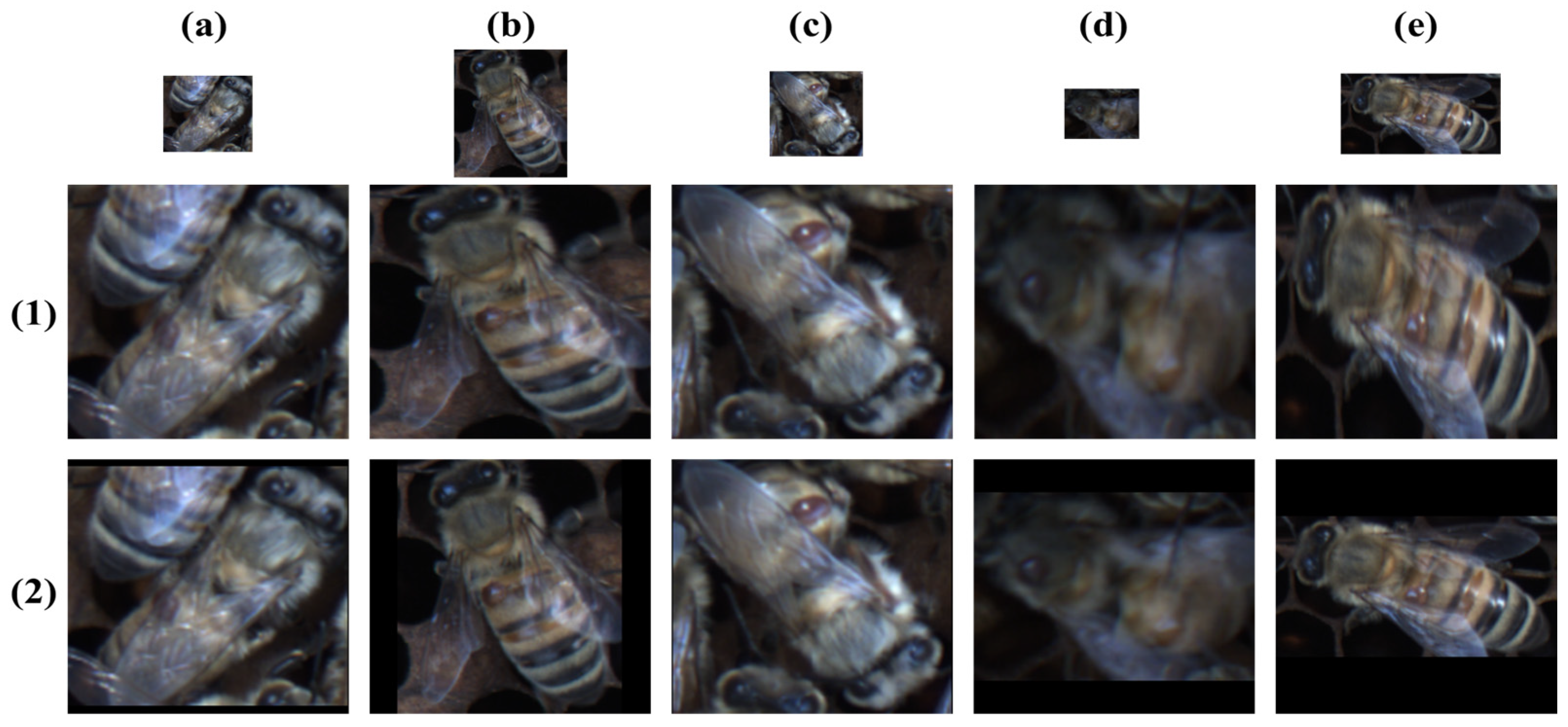
Deep learning computation typically requires input images to have uniform size. In this study, image dimensions were standardized to 224 × 224 pixels, a size that aligns with the input requirements of efficient deep learning architectures, such as MobileNet. Figure 5 shows examples of two image resizing methods. Figure 5(1) shows resizing without preserving bee and Varroa mite morphology, resulting in elongation or thickening compared to the actual shapes. Figure 5(2) shows a method combining resizing and padding to preserve bee and Varroa mite morphology. This method adjusted each image to 224 × 224 pixels while maintaining object morphological characteristics.

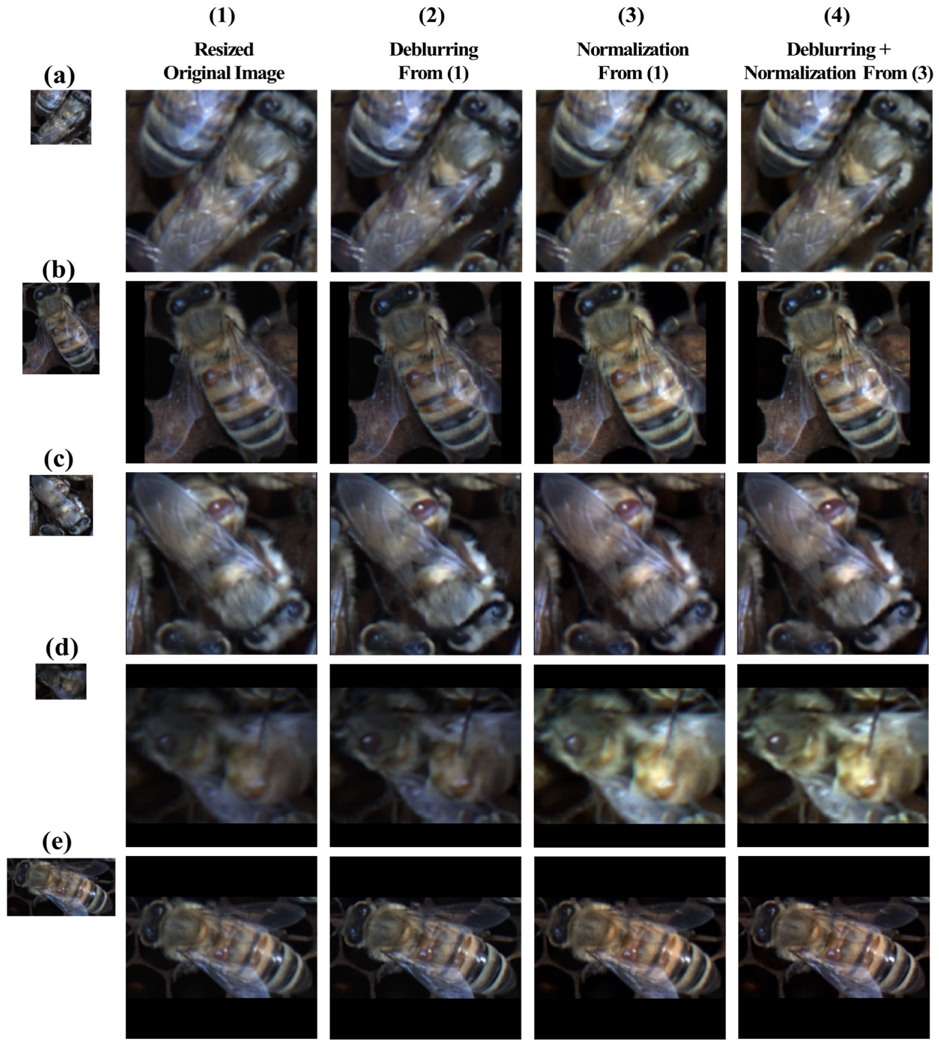
Figure 6 shows the results of deblurring, normalization, and combinations of both image processing techniques applied to Varroa-infested bee images. A comparison of Figure 6(1) and Figure 6(2) indicates that MPRNet-based deblurring of resized images removes overall blurriness and motion artifacts, thus improving texture and detailed structures. Additionally, deblurring complemented unclear pixel information during upscaling of low-resolution regions of interest (Figure 6d). Figure 6(3) shows the results of normalizing resized original images. Here, brightness and contrast were optimized, improving color distribution of bees and Varroa mites. Visualization of yellow and black stripe patterns appearing on bee abdomens was enhanced. Morphological distinction between Varroa mites and host bees was facilitated by such color and pattern sharpening. The combined application of deblurring and normalization resulted in qualitative visual differences that may facilitate entomological classification and pathological observation (Figure 6(4)).

3.2. Quantitative Image Quality Assessment

Table 6. PSNR and MS-SSIM values for normal and Varroa-infested bee images following MPRNet-based deblurring (mean ± std). Differences between normal bee and mite-infested bee images were tested using Welch’s t-test (independent two-sample, unequal variances); n = number of paired ROI images per group.

	Bee	Mite-Infested Bee	p-Value
PSNR (dB)	34.05 (±3.55)	34.34 (±3.65)	p < 0.001
MS-SSIM	0.9832 (±0.0116)	0.9866 (±0.0087)	p < 0.0001

summarizes the PSNR and MS-SSIM values for 3400 images of normal and mite-infested bees after deblurring application. Average PSNR values were 34.05 (±3.55) dB for bee images and 34.34 (±3.65) dB for mite-infested images. For the MS-SSIM, bee images had an average of 0.9832 (±0.0116), while mite-infested images averaged 0.9866 (±0.0087). Statistical analysis confirmed significant differences between bee images and mite-infested images for both PSNR and MS-SSIM metrics (p < 0.001). Particularly for the MS-SSIM, mite-infested images showed MS-SSIM values that were 0.0034 higher than those of normal bee images, indicating superior structural similarity. Both conditions demonstrated excellent performance according to the quality criteria established in Table 2, with the PSNR corresponding to the Very Good grade (30–35 dB) and MS-SSIM to the excellent grade (>0.95). Mite-infested images showed marginally higher PSNR and MS-SSIM means and a lower MS-SSIM standard deviation than normal bee images.

3.3. RGB Channel Analysis in Normal and Varroa Mite-Infested Bees

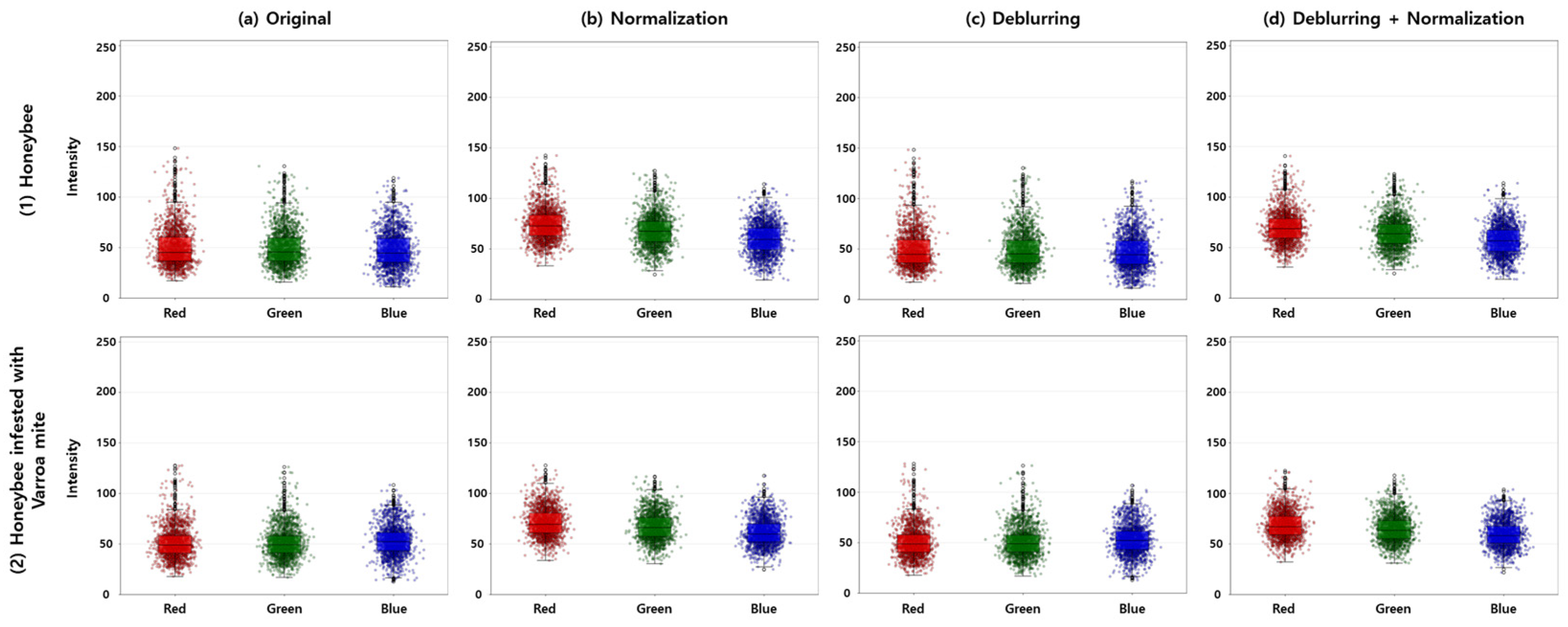
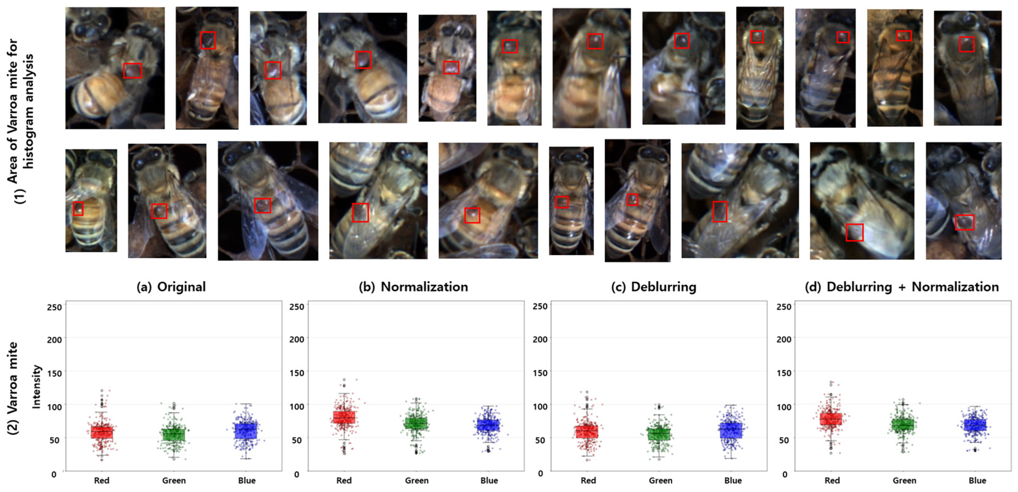
Further insight into spectral characteristics was obtained through RGB channel analysis of normal and mite-infested bee images (Figure 7). In the raw images, the R channel, which contains the principal chromatic information associated with the reddish-brown coloration of Varroa mites, exhibited clear inter-class separation, with corresponding but less pronounced differences observed in the G and B channels (Figure 7a). Mean channel intensities of mite-infested images were higher than those of normal bee images in all three channels, with differences of +1.08 (R), +1.33 (G), and +5.45 (B).

Following histogram normalization, these discriminative spectral relationships were substantially altered. The R-channel difference was reversed from +1.08 to −2.72, with the mean intensity changing from 73.98 in normal images to 71.26 in mite-infested images. In addition, the G-channel difference was reduced by 68% (1.33 to 0.42), and the B-channel difference by 73% (5.45 to 1.49).

Normalization also increased within-image pixel variance across all channels (R: +62%, G: +48%, B: +37%). This indicates that intensity redistribution expanded intra-class variability while reducing inter-class separability. The combined inversion of the R-channel contrast and compression of the G/B-channel differences likely contributed to the reduced classification performance observed after normalization.

The destructive impact of normalization was further confirmed through the extraction of mite-specific pixel distributions (Figure 8). Varroa mite pixel distributions were extracted from the defined ROI regions (Figure 8a) using 335 Varroa-infested bee images selected for their diverse infestation sites—including the abdomen, head, and thorax—and varying degrees of wing occlusion. As shown in the localized histograms (Figure 8b), Varroa mites natively possess lower overall intensity distributions, particularly in the R and G channels, compared to the surrounding bee tissue. While normalization visually enhanced local mite-to-background contrast in these regions, it simultaneously redistributed the global histogram such that the whole-image inter-class variance was minimized. These findings confirm that the R-channel information, vital for identifying the dark red mites, was the most severely compromised by the global normalization process, leading to the instability of classification features.

3.4. Performance of CNN-Based Varroa Mite Identification Models

3.4.1. Overall Performance Across Architectures

Table 7. Classification performance of 19 CNN architectures across 12 preprocessing pipelines (n = 36; 12 datasets × 3 folds per model). Per-dataset breakdowns of accuracy and F1 are provided in Supplementary Tables S1a and S1b, respectively.

Models	Accuracy (%)	F1-Score (%)	Cluster
VarroaNet (r = 8)	97.28 ± 0.59	97.26 ± 0.59	A
VarroaNet (r = 4)	97.15 ± 0.69	97.13 ± 0.70	A
ShuffleNet-V2-x1.0	97.14 ± 0.45	97.11 ± 0.47	A
VarroaNet (r = 16)	97.08 ± 0.57	97.06 ± 0.57	A
GoogLeNet	97.06 ± 1.67	97.04 ± 1.68	A
ShuffleNet-V2-x0.5	96.68 ± 0.97	96.65 ± 0.97	B
EfficientNet-B0	96.31 ± 1.76	96.29 ± 1.74	B
MobileNetV3-Small	95.46 ± 1.61	95.41 ± 1.66	C
RegNet-Y-400MF	95.29 ± 3.75	95.24 ± 3.75	C
MobileNet-V2	93.78 ± 4.27	93.74 ± 4.30	D
DenseNet-121	91.85 ± 5.00	91.79 ± 5.08	D
ResNet-50	88.78 ± 7.92	88.81 ± 7.76	D
ResNet-18	88.09 ± 5.06	87.82 ± 5.31	D
VGG11-BN	60.38 ± 9.65	52.04 ± 19.62	E
MNASNet-1.0	57.90 ± 8.43	49.46 ± 19.21	E
AlexNet	51.10 ± 2.95	35.27 ± 14.97	E
VGG11	50.02 ± 0.02	38.90 ± 21.45	E
Swin Transformer-S	50.00 ± 0.03	27.78 ± 13.81	E
SqueezeNet-1.0	50.00 ± 0.00	0.0 ± 0.0	E

presents the comprehensive performance ranking of the 19 evaluated models across all 12 dataset configurations and three folds (36 validation values per model). Non-converging folds were treated as chance level (50%) and included in the grand mean. Models were grouped into five performance clusters based on natural breaks in the accuracy distribution. A comprehensive synthesis of the overall research findings is tabulated in Supplementary Tables S1a and S2b.

To analyze performance distribution more systematically, the 19 models were categorized into five clusters based on natural breaks in the grand mean accuracy. Cluster A (>97%) contained the top-performing architectures, VarroaNet (r = 8), VarroaNet (r = 4), ShuffleNet-V2-x1.0, VarroaNet (r = 16), and GoogLeNet, all of which consistently achieved high accuracies and F1-scores across most datasets. Cluster B (96–97%) and Cluster C (95–96%) comprised highly capable, lightweight architectures (ShuffleNet-V2-x0.5, EfficientNet-B0, MobileNetV3-Small, RegNet-Y-400MF) that achieved excellent peak performances under optimal preprocessing conditions. Cluster D (80–95%) contained models exhibiting high cross-dataset variance (MobileNetV2, DenseNet-121, ResNet-50, ResNet-18).

Several notable patterns emerged from the per-dataset analysis. ShuffleNet-V2-x1.0 demonstrated the highest robustness to preprocessing variations, maintaining the narrowest accuracy range of 1.41 percentage points (pp) across all 12 datasets (96.15–97.56%). VarroaNet (r = 8) ranked as the second most stable model with a range of 1.91 pp, while notably achieving the highest minimum performance floor among all evaluated models (96.44%). Conversely, performance variance increased markedly in datasets involving normalization. For instance, GoogLeNet and EfficientNet-B0 exhibited performance gaps exceeding 5 pp between their respective best- and worst-performing configurations. RegNet-Y-400MF demonstrated the most extreme sensitivity to preprocessing, with a range of 11.30 pp; its accuracy remained above 97% in all resize-containing datasets but collapsed significantly in the normalization-only (Dataset 2) and deblurring–normalization (Dataset 8) variants. Fold-level standard deviations further indicated that normalization destabilized not only mean performance but also training convergence. While Cluster A models maintained a mean fold standard deviation below 1.0, models in Clusters B and C exhibited pronounced instability in specific configurations, such as MobileNetV3-Small on Dataset 10 and RegNet-Y-400MF on Dataset 2 and Dataset 11.

The six architectures in Cluster E (accuracy < 80%)—VGG11-BN, MNASNet-1.0, AlexNet, VGG11, Swin Transformer-S, and SqueezeNet-1.0—produced near-chance accuracy. SqueezeNet-1.0, Swin Transformer-S, and VGG11 failed to converge in any of the 36 folds, while VGG11-BN, MNASNet-1.0, and AlexNet converged in 41.7%, 44.4%, and 8.3% of folds, respectively. Per the convergence threshold defined in Section 2.6, these architectures were excluded from subsequent analyses.

Kendall’s coefficient of concordance indicated moderate-to-strong agreement in model rankings across preprocessing conditions (W = 0.617, χ² = 88.93, p = 7.95 × 10⁻¹⁴). A two-way ANOVA (13 models × 12 pipelines) showed that architecture accounted for 46.5% of total variance and pipeline for 21.7% (ratio = 2.1), indicating that architecture exerted the dominant effect on classification performance.

3.4.2. Factorial Effects of Preprocessing Combinations

Classification performance across the twelve preprocessing pipelines is summarized for the top nine models (Clusters A–C) in

Table 8. Per-dataset classification accuracy for top 9 models (Clusters A–C), 3-fold CV mean ± std (%). The table matrix is organized continuously to display performance variations under morphology-preserving resizing, non-morphological stretching, and global histogram normalization constraints as defined in the column headers.

Models	Dataset 1	Dataset 2 (N)	Dataset 3 (NR)	Dataset 4 (MR)	Dataset 5 (N, NR)	Dataset 6 (N, MR)
VarroaNet (r = 8)	97.32 ± 0.71	96.76 ± 0.25	98.35 ± 0.67	97.73 ± 0.49	98.12 ± 0.53	97.47 ± 0.46
VarroaNet (r = 4)	97.29 ± 0.89	96.62 ± 0.15	97.77 ± 0.69	97.32 ± 0.85	98.20 ± 0.52	97.00 ± 0.47
ShuffleNet-V2-x1.0	97.21 ± 0.37	96.29 ± 0.75	97.56 ± 0.67	97.09 ± 0.58	97.47 ± 0.60	97.26 ± 0.40
VarroaNet (r = 16)	97.06 ± 0.36	96.94 ± 0.30	97.79 ± 0.44	97.53 ± 0.19	97.73 ± 0.69	97.06 ± 0.93
GoogLeNet	97.56 ± 0.53	95.44 ± 1.06	98.44 ± 0.15	97.94 ± 0.04	97.65 ± 0.49	97.73 ± 0.54
ShuffleNet-V2-x0.5	96.26 ± 0.54	95.03 ± 0.55	97.94 ± 0.44	96.59 ± 0.29	97.79 ± 0.47	96.80 ± 0.18
EfficientNet-B0	96.41 ± 1.23	92.47 ± 2.33	97.94 ± 0.51	94.59 ± 4.29	97.79 ± 0.89	96.97 ± 0.64
MobileNetV3-Small	96.44 ± 0.23	93.79 ± 1.05	96.97 ± 1.19	96.38 ± 0.73	96.94 ± 0.65	95.91 ± 1.38
RegNet-Y-400MF	94.20 ± 5.09	86.76 ± 5.08	98.06 ± 0.14	97.68 ± 0.40	97.65 ± 0.68	97.82 ± 0.18
Models	Dataset 7 (D)	Dataset 8 (D, N)	Dataset 9 (D, NR)	Dataset 10 (D, MR)	Dataset 11 (D, N, NR)	Dataset 12 (D, N, MR)
VarroaNet (r = 8)	96.50 ± 0.46	96.44 ± 0.04	97.44 ± 0.33	97.14 ± 0.29	97.12 ± 0.70	96.97 ± 0.98
VarroaNet (r = 4)	97.03 ± 0.16	95.38 ± 0.73	97.47 ± 0.32	97.09 ± 0.45	97.56 ± 0.54	97.09 ± 0.13
ShuffleNet-V2-x1.0	97.38 ± 0.23	96.15 ± 0.60	97.38 ± 0.63	97.27 ± 0.63	97.47 ± 0.24	97.15 ± 0.47
VarroaNet (r = 16)	96.70 ± 0.70	95.79 ± 0.60	97.38 ± 0.71	97.00 ± 0.40	97.50 ± 0.74	96.50 ± 0.43
GoogLeNet	97.35 ± 0.36	92.29 ± 3.10	98.00 ± 0.40	97.59 ± 0.49	97.71 ± 0.63	97.00 ± 0.71
ShuffleNet-V2-x0.5	95.91 ± 0.33	95.09 ± 1.02	97.47 ± 0.11	97.41 ± 0.51	97.17 ± 0.33	96.64 ± 0.50
EfficientNet-B0	97.12 ± 0.79	94.82 ± 0.48	97.73 ± 0.49	94.62 ± 4.31	97.59 ± 0.90	97.68 ± 0.40
MobileNetV3-Small	96.94 ± 0.67	93.26 ± 0.49	93.56 ± 5.64	95.88 ± 0.71	96.62 ± 0.81	92.82 ± 4.24
RegNet-Y-400MF	96.21 ± 0.37	89.50 ± 3.57	97.94 ± 0.40	97.50 ± 0.47	97.18 ± 1.13	92.97 ± 5.14

N (normalization); NR (non-morphological resize); MR (morphology-preserving resize); D (deblurring).

, organized under the 2 × 2 × 3 factorial design (deblurring, normalization, resizing) described in Section 2.6.

The 12 preprocessing configurations were ranked by mean accuracy across the 13 working models within Clusters A through D. Pipelines containing resizing consistently achieved the highest rankings, with Dataset 4 (MR: 97.48%) and Dataset 3 (NR: 96.74%) emerging as the top-performing configurations for the original-source datasets. In contrast, Dataset 2 (normalization only: 90.86%) and Dataset 8 (deblurring and normalization: 90.82%) ranked the lowest, substantially underperforming even the unprocessed baseline images, which recorded 94.59% (Dataset 1) and 94.09% (Dataset 7). This ranking remained consistent across both original and deblurred source conditions, confirming that resizing was the single most beneficial preprocessing step, while normalization alone proved to be actively harmful to classification performance. To further isolate the contribution of each preprocessing factor, single-factor effects were quantified using the Wilcoxon signed-rank test and Cohen’s d across the 13 working models, as summarized in

Table 9. Varroa mite classification performance across factorial preprocessing combinations. Each cell is the mean +/− SD classification accuracy (%) across the 13 working models for the given preprocessing combination.

Processing	Accuracy (%)
	Non-Resize	Non-Morphological Resize	Morphology-Preserving Resize
Original	94.59 ± 4.22	96.74 ± 2.35	97.48 ± 0.93
Normalization	90.86 ± 6.87	94.86 ± 4.04	95.03 ± 4.82
Deblurring	94.09 ± 5.15	96.96 ± 1.30	97.11 ± 1.12
Deblurring and Normalization	90.82 ± 5.88	93.94 ± 4.35	94.71 ± 4.03

. For the evaluation of resizing methods, effects relative to the no-resize baseline—calculated as the mean of Datasets 1, 2, 7, and 8—were computed separately to clarify their individual impact. Single-factor effects and two-way interactions were quantified using the Wilcoxon signed-rank test and Cohen’s d across the 13 evaluated architectures.

Resizing produced the largest single-factor effect on classification accuracy (

Table 10. Main effects of individual preprocessing factors on classification accuracy. Values represent mean accuracy difference (Δ pp ± std) relative to the no-resize baseline (mean of Datasets 1, 2, 7, and 8 for the resize factors, corresponding non-deblurred/non-normalized baselines for the other factors), tested with the Wilcoxon signed-rank test (n = 13 working models).

Processing	Accuracy (%)	Cohen’s d	p-Value	Significance
MR	+3.49 ± 3.62	0.96	0.000244	***
NR	+3.04 ± 2.86	1.06	0.000244	***
Normalization	−2.79 ± 3.07	−0.91	0.000244	***
Deblurring	−0.32 ± 0.62	−0.52	0.068	n.s.

NR (non-morphological resize); MR (morphology-preserving resize); n.s., p ≥ 0.05; *** p < 0.001.

). Both MR (d = 0.96, p < 0.001) and NR (d = 1.06, p < 0.001) exceeded the threshold for large effect sizes, consistent with the wide variation in original ROI dimensions (40 × 39 to 344 × 302 pixels; mean 112 × 126 pixels). The magnitude of the resize benefit was inversely related to baseline model performance: VarroaNet (r = 8) gained 0.79 pp, whereas DenseNet-121 gained 10.09 pp. In contrast, global histogram normalization reduced mean accuracy by 2.79 ± 3.07 pp (d = −0.91, p < 0.001), with degradation observed in 12 of the 13 evaluated architectures.

The 11.46 pp decline in ResNet-50 under normalization indicated that higher-capacity architectures were more sensitive to spectral redistribution than lightweight counterparts. MPRNet-based deblurring did not produce a statistically significant accuracy gain (p = 0.068).

Although both resizing methods individually exhibited large effect sizes (MR: d = 0.96; NR: d = 1.06), no statistically significant difference was detected between the two protocols (

Table 11. Pairwise comparison of morphology-preserving (MR) and non-morphological (NR) resize methods. Values represent mean accuracy difference (Δ pp ± std) of MR minus NR, tested with the Wilcoxon signed-rank test (n = 13 working models).

Processing	Accuracy (%)	Cohen’s d	p-Value	Significance
Contrast of MR and NR	+0.45 ± 1.98	0.23	0.376	n.s.

NR (non-morphological resize); MR (morphology-preserving resize); n.s., p ≥ 0.05.

; p = 0.376). This finding indicates that uniform spatial standardization, irrespective of the rescaling algorithm applied, constitutes the primary determinant of classification improvement.

The normalization × resize interaction was significant (p = 0.040,

Table 12. Normalization × resize interaction effects on classification accuracy. Values represent mean accuracy difference (Δ pp ± std) introduced by normalization within each resize condition, tested with the Wilcoxon signed-rank test (n = 13 working models).

Processing	Accuracy (%)	Cohen’s d	p-Value	Significance
Normalization, non-resize	−3.50 ± 3.72	−0.94	0.001	**
Normalization, NR	−2.46 ± 3.00	−0.82	0.000244	***
Normalization, MR	−2.42 ± 3.90	−0.62	0.008	**
Normalization, resize interaction (interaction paired)	−1.06 (no rz − rz)	-	0.040	*

NR (non-morphological resize); MR (morphology-preserving resize); * p < 0.05; ** p < 0.01; *** p < 0.001.

). The normalization penalty decreased monotonically as resizing was introduced—from −3.50 pp (d = −0.94) without resizing to −2.44 pp (d = −0.62) under MR—and the resize benefit was correspondingly larger when applied alongside normalization.

The deblurring × normalization interaction was not significant (p = 0.340,

Table 13. Deblurring × normalization interaction effects on classification accuracy. Values represent mean accuracy difference (Δ pp ± std) introduced by deblurring within each normalization condition, tested with the Wilcoxon signed-rank test (n = 13 working models).

Processing	Accuracy (%)	Cohen’s d	p-Value	Significance
Deblurring, non-normalization	−0.22 ± 1.22	-	-	n.s.
Deblurring, normalization	−0.43 ± 1.94	-	-	n.s.
Deblurring (interaction paired)	+0.21	-	0.340	n.s.

n.s., p ≥ 0.05.

). Deblurring produced small negative effects both without (−0.22 pp) and with (−0.43 pp) normalization, neither of which reached significance. Cross-model standard deviations (Table 9) were consistently higher in normalization-containing pipelines (e.g., Dataset 2: ± 6.87) than in their unnormalized counterparts (Dataset 1: ± 4.22), indicating that normalization increased between-model variability in addition to reducing mean accuracy. Among all twelve pipelines, MR alone (Dataset 4) yielded the highest mean accuracy (97.48%).

3.5. Multi-Resolution Analysis of Varroa Mite Detection: Classification and Explainability

To elucidate the decision-making behavior of the trained backbones across varying spatial scales, a multi-resolution analysis was conducted using the six selected architectures. Additional results related to model development are provided in Supplementary Table S2. The selected models were evaluated across four feature map resolutions (7 × 7, 14 × 14, 28 × 28, and 56 × 56) under a balanced factorial design. The complete experimental matrix comprised 864 training runs for classification and 288 single-split runs for Grad-CAM++ generation.

Table 14. Effect of feature map resolution on Varroa mite classification accuracy, averaged across the 12 preprocessing pipelines per architecture (mean ± std; n = 36 per cell from 12 pipelines × 3 folds).

Architecture	Res. 7 × 7	Res. 14 × 14	Res. 28 × 28	Res. 56 × 56
ShuffleNet-V2-x1.0	97.21 ± 0.5	97.34 ± 0.5	97.14 ± 0.5	95.85 ± 2.6
ShuffleNet-V2-x0.5	96.79 ± 0.8	96.92 ± 1.0	97.24 ± 0.8	96.18 ± 2.5
MobileNetV3-Small	95.88 ± 1.2	96.10 ± 1.1	96.41 ± 1.0	84.79 ± 13.5
EfficientNet-B0	95.80 ± 2.3	96.03 ± 2.8	96.31 ± 2.3	96.52 ± 2.8
VarroaNet (r = 4)	97.21 ± 0.6	97.31 ± 0.5	97.22 ± 0.6	96.16 ± 3.1
VarroaNet (r = 8)	97.20 ± 0.5	97.22 ± 0.4	97.26 ± 0.6	95.69 ± 2.5

summarizes the mean classification accuracies for each architecture–resolution configuration.

3.5.1. Impact of Feature Map Resolution on Classification Robustness

Relative to the 7 × 7 baseline, mean accuracy increased by +0.14 pp at 14 × 14 (win/loss = 42/29), increased by +0.25 pp at 28 × 28 (44/27), and decreased by −2.48 pp at 56 × 56. The overall Kruskal–Wallis test was not significant (H = 1.862, p = 0.602); the median performance remained stable at 97.15% across all resolutions, with the mean drawn down by the collapse of MobileNetV3-Small at 56 × 56 (84.79%).

A three-way η² decomposition of the six architecture × four resolution × 12 pipeline matrix (288 cells) attributed 13.3% of total variance to pipeline, 11.1% to architecture, and 8.4% to resolution, with 67.1% residual variance and higher-order interactions.

The MobileNetV3-Small collapse at 56 × 56 was pipeline-selective: the normalization-only pipeline (Dataset 2: 63.06%) and the original unprocessed inputs (Dataset 1: 81.70%) degraded severely, whereas resize-containing pipelines (NR-only: 97.76%; deblurring with MR: 97.41%) remained near the 7 × 7 baseline. Training accuracy at 56 × 56 averaged only 86.09% (σ = 18.58), with single-split validation and test accuracies of 84.26% and 82.01%, respectively. EfficientNet-B0 was the only architecture to gain accuracy at 56 × 56 (+0.73 pp). Sensitivity analysis with non-converging folds excluded (Table S6) yielded an aggregate accuracy of 87.86% (Δ = +3.07 pp), which does not alter the principal conclusion that 56 × 56 destabilizes MobileNetV3-Small under spectrally homogenized inputs.

Resolution sensitivity differed across architectures. High-performing models at 7 × 7 (>97.2%; VarroaNet (r = 4, 8); ShuffleNet-V2-x1.0) showed negligible change at 28 × 28 (+0.00 to +0.06 pp). Lower-baseline models gained +0.52 to +0.54 pp at 28 × 28. Per-architecture Kruskal–Wallis tests on resolution deltas (Δ vs. 7 × 7) reached significance only at 28 × 28 (H = 12.36, p = 0.030; 14 × 14: p = 0.50; 56 × 56: p = 0.19).

Inference latency varied by less than 2 ms across resolutions (

Table 15. Computational efficiency and inference latency across architectures and resolutions.

Architecture	Latency (ms) Res. 7 × 7	Latency (ms) Res. 14 × 14	Latency (ms) Res. 28 × 28	Latency (ms) Res. 56 × 56
ShuffleNet-V2-x1.0	9.73	9.41	10.15	10.46
ShuffleNet-V2-x0.5	9.25	9.15	9.59	10.98
MobileNetV3-Small	7.99	7.99	8.03	8.11
EfficientNet-B0	12.75	12.04	12.57	13.04
VarroaNet (r = 4)	10.78	9.91	10.78	11.33
VarroaNet (r = 8)	10.35	10.94	10.77	11.57

). Training cost per fold rose from 266 s at 7 × 7 to 298 s at 28 × 28 (+12%) and 1067 s at 56 × 56 (+301%); the 56 × 56 condition consumed approximately 64 GPU-hours across its 72 configurations.

For an independent assessment using the fixed 7:2:1 single split, Supplementary Table S3 reports per-architecture validation–test accuracy gaps; these range from 1.2 to 2.7 pp (all Wilcoxon p < 0.001), consistent with the absence of catastrophic overfitting under the k-fold protocol used throughout this section.

Pipeline rankings were stable across all four resolutions (Friedman test, p < 0.001 at each resolution): MR and NR pipelines occupied the top two ranks, and normalization-only configurations the lowest. Sensitivity to normalization scaled with resolution: the mean normalization penalty grew from −1.67 pp at 7 × 7 to −8.50 pp at 56 × 56 (range: −20.7 to −4.5).

3.5.2. Spatial Attribution and Localization Fidelity Across Resolutions

To evaluate the spatial precision of model decision-making, localization metrics derived from Grad-CAM++ heatmaps were analyzed across four feature map resolutions. The aggregate localization performance across the six evaluated architectures is summarized in

Table 16. Aggregate localization quality metrics across feature map resolutions, averaged across 6 architectures and 12 preprocessing pipelines (n = 72 per resolution; computed on the 170 mite-infested test images). Distance ↓ denotes lower is better.

Resolution	IoU@50	IoU@30	Pointing Game	Energy Inside	Distance↓	n_arch
7 × 7	0.211	0.173	0.361	0.154	0.101	6
14 × 14	0.241	0.201	0.354	0.200	0.092	6
28 × 28	0.286	0.268	0.438	0.289	0.080	6
56 × 56	0.151	0.205	0.274	0.276	0.140	6

.

Four of five localization metrics (IoU@50, IoU@30, Energy Inside, and distance error) improved monotonically from 7 × 7 to 28 × 28, with a marked regression at 56 × 56. The Pointing Game score showed a marginal dip at 14 × 14 (0.3536 vs. 0.3613 at 7 × 7) before reaching its peak at 28 × 28 (0.4381). The 28 × 28 resolution yielded the best overall performance across all five metrics: IoU@50 = 0.2857, IoU@30 = 0.2686, Pointing Game = 0.4381, Energy Inside = 0.2885, and distance error = 0.0804. The Kruskal–Wallis tests on per-configuration means (n = 72; 6 architectures × 12 pipelines per resolution) confirmed statistically significant resolution effects for all five metrics: IoU@50 (H = 30.40, p < 0.001), IoU@30 (H = 14.98, p = 0.002), Pointing Game (H = 11.17, p = 0.011), Energy Inside (H = 27.43, p < 0.001), and distance error (H = 22.24, p < 0.001). Among the five metrics, Pointing Game produced the smallest H statistic, reflecting a marginal performance dip at 14 × 14 (0.354 vs. 0.361 at 7 × 7) before reaching its peak at 28 × 28 (0.438).

The performance decline at 56 × 56 is attributable to the excessive spatial dispersion of activations. While a 7 × 7 feature map contains only 49 candidate locations and therefore enforces competitive, concentrated responses, a 56 × 56 map contains 3136 locations, allowing activations to fragment into multiple sub-regions. This reduces the peak-to-background contrast of the saliency map and degrades threshold-based localization precision.

This trend is further supported by receptive-field interpretation. At a 28 × 28 resolution, each feature cell corresponds to approximately an 8 × 8 pixel region within the 224 × 224 input image. Under the present acquisition conditions, Varroa mites (approximately 1.1 × 1.6 mm) occupy roughly 10–20 pixels, meaning that 1–4 adjacent cells at 28 × 28 can effectively represent the target. By contrast, the 7 × 7 resolution (32 × 32 pixels per cell) is overly coarse, whereas the 56 × 56 resolution (4 × 4 pixels per cell) is excessively granular and more sensitive to high-frequency noise.

Per-architecture analysis revealed three distinct localization response patterns (

Table 17. Architecture-specific localization performance at each feature map resolution, averaged across the 12 preprocessing pipelines per architecture–resolution cell (n = 36 per cell from 12 pipelines × 3 folds; computed on the 170 mite-infested test images). Distance ↓ denotes lower is better.

Architecture	Resolution	IoU@50	IoU@30	Pointing Game	Energy Inside	Distance ↓
VarroaNet (r = 4)	7 × 7	0.185	0.162	0.317	0.149	0.078
	14 × 14	0.319	0.277	0.523	0.292	0.058
	28 × 28	0.309	0.301	0.483	0.327	0.063
	56 × 56	0.121	0.184	0.259	0.292	0.086
VarroaNet (r = 8)	7 × 7	0.213	0.170	0.371	0.156	0.075
	14 × 14	0.190	0.166	0.216	0.165	0.086
	28 × 28	0.387	0.349	0.691	0.385	0.045
	56 × 56	0.126	0.211	0.285	0.328	0.107
ShuffleNet-V2-x1.0	7 × 7	0.237	0.194	0.400	0.176	0.075
	14 × 14	0.208	0.160	0.359	0.164	0.081
	28 × 28	0.258	0.227	0.308	0.240	0.078
	56 × 56	0.094	0.174	0.159	0.254	0.096
ShuffleNet-V2-x0.5	7 × 7	0.239	0.227	0.396	0.207	0.072
	14 × 14	0.324	0.270	0.439	0.275	0.066
	28 × 28	0.385	0.368	0.513	0.386	0.064
	56 × 56	0.267	0.335	0.492	0.420	0.072
MobileNetV3-Small	7 × 7	0.245	0.170	0.401	0.135	0.116
	14 × 14	0.235	0.189	0.344	0.167	0.115
	28 × 28	0.189	0.180	0.190	0.179	0.113
	56 × 56	0.122	0.126	0.175	0.139	0.304
EfficientNet-B0	7 × 7	0.149	0.118	0.286	0.106	0.190
	14 × 14	0.171	0.144	0.243	0.140	0.142
	28 × 28	0.184	0.185	0.442	0.212	0.121
	56 × 56	0.186	0.215	0.294	0.248	0.162

). First, channel-shuffle-based architectures, including ShuffleNet-V2 and VarroaNet (r = 8), consistently achieved peak localization performance at the 28 × 28 resolution. Paired t-tests between VarroaNet (r = 4) and VarroaNet (r = 8) indicated no significant classification differences across all four resolutions (all p > 0.36). TOST equivalence at δ = ±1.0 pp was confirmed for the 7 × 7, 14 × 14, and 28 × 28 resolutions (all p_TOST < 0.001), whereas equivalence could not be established at 56 × 56 (p_TOST = 0.209; 90% CI = [−0.82, +1.77]), reflecting elevated cross-pipeline variance at this resolution (Table S5). However, a localization crossover was identified: full SE (r = 4) yielded a substantially higher IoU at 14 × 14 (IoU@30: 0.277 vs. 0.166, Δ = +0.111, p < 0.001), whereas r = 8 was superior at 7 × 7, 28 × 28, and 56 × 56 (28 × 28 IoU@30: 0.349 vs. 0.301; PG: 0.691 vs. 0.483; both p < 0.001). This pattern indicates that strong channel compression (r = 4) uniquely aids spatial focus at the 14 × 14 resolution, where moderate spatial detail combines with aggressive channel recalibration, whereas at other resolutions the weaker compression (r = 8) maintains a more balanced spatial-channel representation.

Among all evaluated configurations, VarroaNet (r = 8) produced the highest Pointing Game score (0.691) and the lowest distance error (0.045), indicating superior target centering and spatial precision. Second, VarroaNet (r = 4), which incorporates full squeeze-and-excitation recalibration, reached its optimum at 14 × 14 and declined thereafter, suggesting that stronger channel attention might become over-selective at finer spatial grids. Third, EfficientNet-B0 and MobileNetV3-Small displayed heterogeneous behaviors, with different metrics peaking at different resolutions and generally lower IoU consistency, reflecting diffuse or unstable attribution patterns. Collectively, these findings indicate that localization fidelity depends not only on spatial resolution but also on the interaction between resolution and architectural inductive bias.

Robustness analysis across all 48 per-architecture configurations (four resolutions × 12 pipelines) identified VarroaNet (r = 8) as the most stable model, with the lowest coefficient of variation (CV = 1.47%), a performance range of 7.1 percentage points, and a mean accuracy of 96.84%. ShuffleNet-V2-x1.0 and ShuffleNet-V2-x0.5 showed the next highest stability (CV = 1.52% each). In contrast, MobileNetV3-Small exhibited the highest variability (CV = 8.87%). When 56 × 56 configurations were excluded, its CV decreased to 2.15%, approaching that of EfficientNet-B0 (2.26%), indicating that the observed instability was strongly associated with the highest resolution condition.

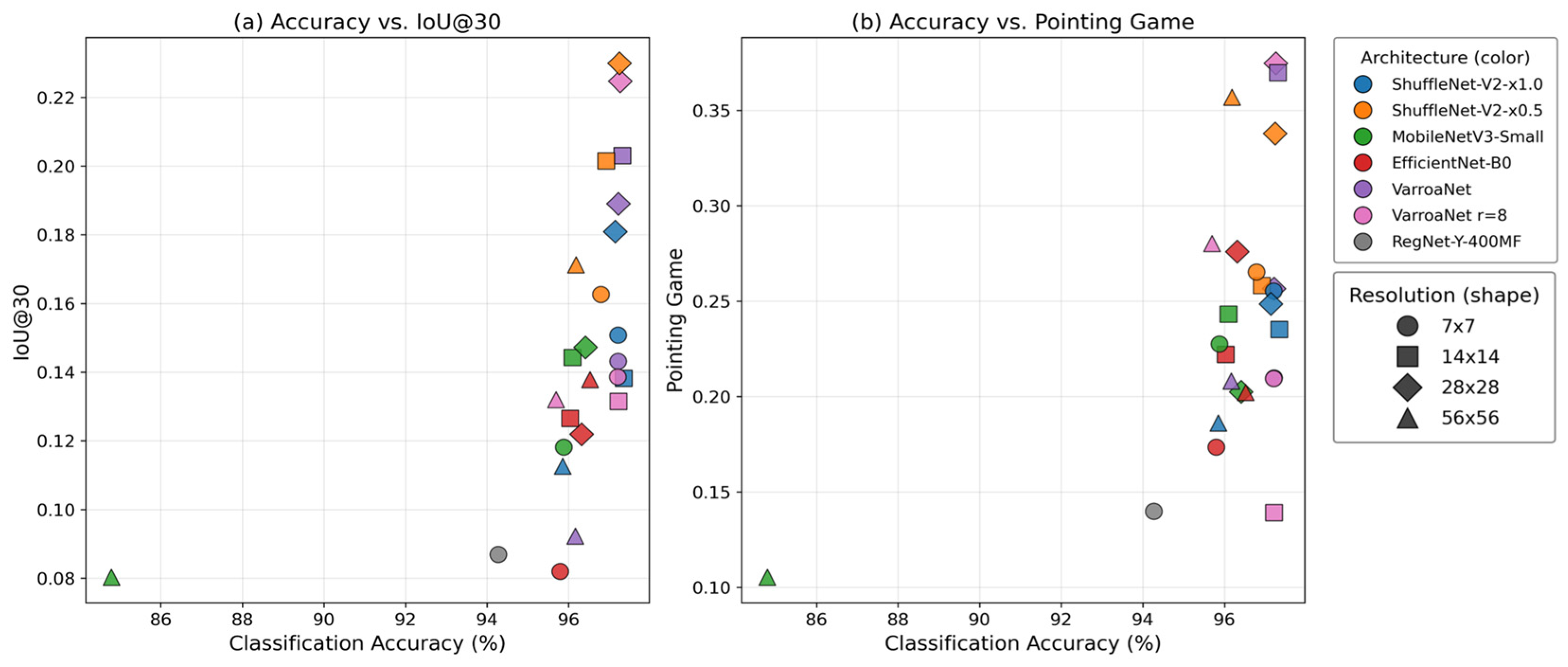
To test whether classification accuracy serves as a reliable proxy for localization fidelity, classification accuracy and localization fidelity were not in strict correspondence, as visualized in Figure 9; to formally test this, Spearman rank correlations were computed across the 24 (architecture × resolution) configurations between mean accuracy and each localization metric. Three of the five metrics—distance error (ρ = −0.745), IoU@50 (ρ = +0.647), and Pointing Game (ρ = +0.565)—showed significant positive concordance after Holm–Bonferroni correction (all adjusted p ≤ 0.013), whereas IoU@30 and Energy Inside did not (Table S4). Even the strongest coefficient leaves substantial variance unexplained, and rank-level dissociations confirm the limitation: the highest-accuracy configuration (ShuffleNet-V2-x1.0 at 14 × 14, 97.34%) ranked 21st of 24 in IoU@30, while the configuration with the highest Pointing Game (VarroaNet (r = 8) at 28 × 28) ranked only third in accuracy. Accuracy is therefore a partially informative but insufficient surrogate for spatial attribution quality, supporting the use of explicit localization metrics for deployment-oriented model selection.

3.5.3. Qualitative Verification via Grad-CAM++ Visualization

Grad-CAM++ heatmaps were qualitatively inspected to verify that the quantitative localization results were not driven by spurious correlations or structural aliasing [59]. This approach confirms the robustness of the XAI representations across the different resolution scales evaluated in the preceding performance analysis.

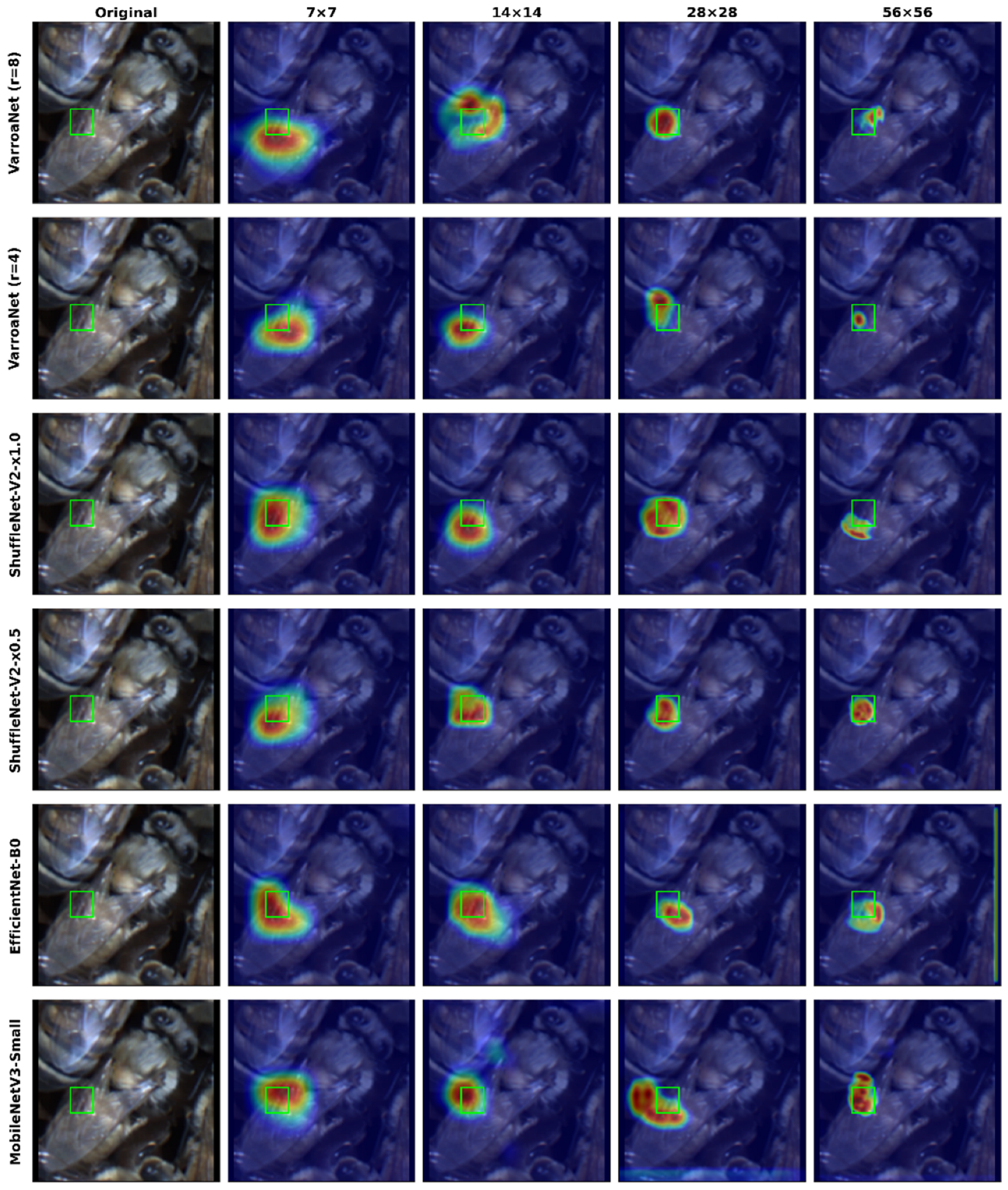
Figure 10 presents the Grad-CAM++ heatmap visualization for all six architectures across four feature map resolutions on a representative mite-infested image from Dataset 10. Three resolution-dependent patterns are visually evident. At 7 × 7, all architectures produce broad activation regions encompassing the entire bee body, with limited spatial specificity for the mite. At 28 × 28, channel-shuffle-based architectures (VarroaNet (r = 8), ShuffleNet-V2-x0.5) generated tightly focused heatmaps precisely localized on the mite body, consistent with their quantitative superiority (VarroaNet (r = 8): PG = 0.691, IoU@30 = 0.349; ShuffleNet-V2-x0.5: PG = 0.513, IoU@30 = 0.368). In contrast, EfficientNet-B0 and MobileNetV3-Small exhibited more diffuse activation patterns extending to surrounding body regions and background comb structures. At 56 × 56, activations fragmented into multiple sub-mite patches for most architectures, visually confirming the quantitative localization regression observed in Table 16.

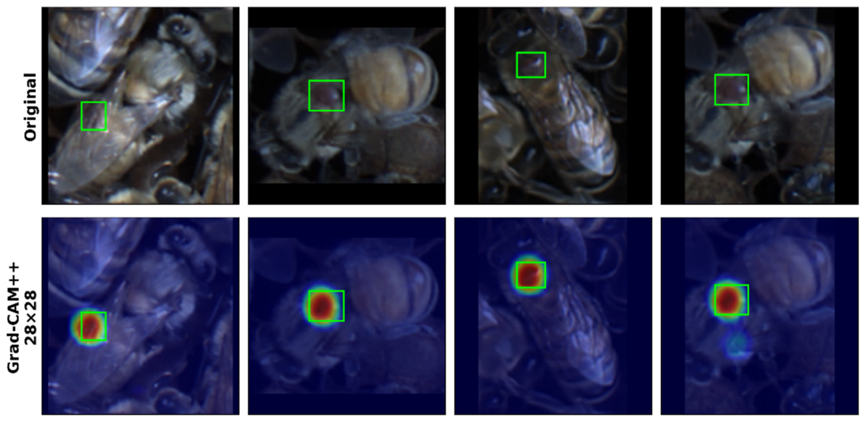
Figure 11 demonstrates the consistency of VarroaNet (r = 8) at 28 × 28 with deblurring + MR preprocessing across eight diverse test images with varying bee postures, mite attachment sites, and background conditions. For each example shown, the Grad-CAM++ activation peak coincided with the annotated mite bounding box, consistent with this configuration’s Pointing Game accuracy of 92.7% across the 170 mite-infested test images. This robust spatial precision, combined with the lowest distance error (0.045, normalized by image diagonal) of any configuration, confirms that VarroaNet (r = 8) at 28 × 28 with deblurring + MR localizes mite-specific features rather than relying on contextual cues such as wing deformation or body discoloration.

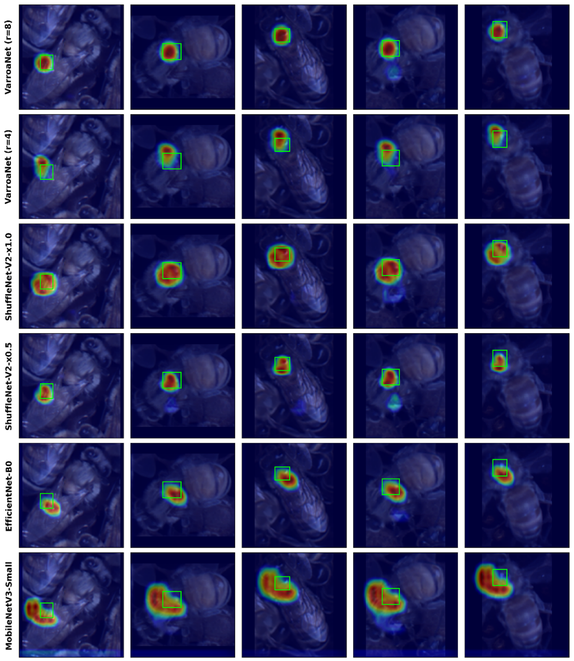
Figure 12 further illustrates inter-architecture variation at 28 × 28 across multiple test images: channel-shuffle-based architectures consistently produced focused activations on the mite region, whereas EfficientNet-B0 and MobileNetV3-Small generated spatially dispersed heatmaps with activation extending to non-mite regions, reflecting their lower quantitative localization scores (EfficientNet-B0 PG = 0.442; MobileNetV3-Small PG = 0.190 at 28 × 28). A consolidated overview of all six architectures at 28 × 28 on representative test images is provided in Figure S1. The SE channel attention reversal was also visually apparent: at 14 × 14, VarroaNet (r = 4) (full SE) produced more concentrated activations than r = 8 (PG: 0.523 vs. 0.216), whereas at 28 × 28, r = 8 produced a markedly tighter spatial focus (PG: 0.691 vs. 0.483), corroborating the quantitative crossover reported in Section 3.5.2.

3.5.4. Preprocessing Effects on Localization Quality

The preprocessing pipeline significantly affected Grad-CAM++ localization quality, with the resize method as the dominant factor. Cohen’s d effect sizes for IoU@30 (per-configuration means; n = 72 per condition) revealed substantial improvements relative to Dataset 1 (the original, unresized images), with d = 2.09 for NR and d = 1.61 for MR; the difference between the two resize strategies was modest (d = 0.34; all p < 0.001). Deblurring had no significant main effect (d = +0.006, p = 0.81), and normalization had a negligible negative effect (d = −0.036). These patterns parallel the classification findings (Section 3.4): resize is the dominant beneficial factor for both classification accuracy and localization quality.

NR produced higher raw localization scores than MR across all six architectures (mean IoU@30: 0.291 vs. 0.252). However, a geometric measurement bias partially explains this advantage. NR stretches images to fill the entire 224 × 224 canvas, enlarging the ground-truth bounding box to a mean coverage of 2.61% of the image area, whereas MR preserves the original aspect ratio with center padding, producing a smaller bounding box coverage of 1.72% (ratio: 1.52×). This larger target region under NR inherently increases the probability of overlap between the bounding box and the thresholded CAM activation, inflating area-based metrics independently of actual localization precision. When IoU@30 was normalized by bounding box coverage, MR exhibited 29% higher area-normalized efficiency (14.30 vs. 11.03). Furthermore, NR introduced a mean aspect ratio distortion of 47.5% (computed as |1 − w/h| × 100, where w and h denote the original ROI width and height), with 73.9% of images exhibiting >20% distortion, deforming the morphological features that biologists rely on for visual validation.

A deblurring × resize interaction was identified. Without deblurring, NR substantially outperformed MR (IoU@30: 0.304 vs. 0.232, Δ = 0.072), but with deblurring, the gap narrowed considerably (0.272 vs. 0.261, Δ = 0.011). This interaction suggests that deblurring enhances edge definition, which particularly benefits the aspect-ratio-preserving resize method where mite boundary information is spatially accurate. For the Pointing Game, MR improved from 0.365 without deblurring to 0.451 with deblurring (Δ = +0.086, +24%), whereas NR showed a slight decrease (0.495 to 0.472).

At the model × pipeline × resolution level, the top MR configurations were ShuffleNet-V2-x0.5 at 56 × 56 with deblurring + MR (IoU@30 = 0.548), VarroaNet (r = 8) at 28 × 28 with deblurring + MR (IoU@30 = 0.510, PG = 0.927), and VarroaNet (r = 4) at 28 × 28 with MR (IoU@30 = 0.507). The VarroaNet (r = 8) configuration achieved a Pointing Game of 0.927 (n = 170 mite-infested test images), indicating that in 92.7% of test images, the Grad-CAM++ activation peak fell directly within the annotated mite bounding box. Under the full preprocessing pipeline (deblurring + normalization + MR), VarroaNet (r = 8) at 56 × 56 achieved an IoU@30 = 0.505 with PG = 0.865.

The top MR-based configuration (VarroaNet (r = 8) at 28 × 28 with deblurring + MR) achieved an IoU@30 = 0.510 and PG = 0.927, while the top NR-based configuration (ShuffleNet-V2-x0.5 at 28 × 28) reached the highest overall IoU@30 (0.368).

4. Discussion

This study systematically examined how preprocessing strategy, model architecture, and feature map resolution influence classification accuracy and explainability in Varroa mite image recognition. Across all experiments, three consistent findings emerged: (1) simpler preprocessing pipelines outperformed more complex combinations, (2) architecture selection had a greater impact than preprocessing choice, and (3) an intermediate feature map resolution (28 × 28) provided the best balance between predictive performance and localization quality. These results have important implications for the selection of preprocessing strategies and model architectures in small-scale agricultural image classification.

First, the preprocessing analysis demonstrated that additional image enhancement does not necessarily improve performance. Resize-only pipelines consistently achieved the highest classification accuracy, whereas adding normalization or deblurring often reduced performance. This finding contrasts with the common practice of stacking multiple preprocessing steps without validating their individual contributions. The negative effect of normalization is consistent with the RGB channel analysis in Section 3.3: global histogram redistribution inverted the R-channel inter-class difference (+1.08 → −2.72) and compressed the G/B-channel separation by 68% and 73%, while inflating intra-class variance. Under these conditions, normalization removed rather than enhanced the chromatic cues required to distinguish reddish-brown mites from bee tissue. The amplification of the normalization penalty at higher resolutions (−1.67 pp at 7 × 7 → −8.50 pp at 56 × 56) reinforces this interpretation: finer feature maps would otherwise resolve the inter-class chromatic gradients that global normalization removes, and the cost of this removal scales with spatial granularity. In practical terms, preprocessing should be treated as a hypothesis requiring empirical validation rather than as a universally beneficial routine. This perspective is consistent with previous observations that empirical transformations or data augmentations do not automatically guarantee complete model invariance to spatial variations [60]. The limited benefit of deblurring in this study likely reflects the dataset curation step (Section 2.1), which excluded severely blurred frames prior to preprocessing; under such conditions, the residual motion blur was insufficient to bottleneck classification, and the high-frequency textural modifications introduced by MPRNet did not align with the features used by the CNN backbones.

Second, model architecture exerted a larger influence on performance than preprocessing condition. Model rankings were relatively stable across pipelines, and variance decomposition consistently showed that architecture explained substantially more performance variation than preprocessing. Lightweight CNNs such as VarroaNet and ShuffleNet performed best, whereas heavily parameterized networks such as VGG11 failed to converge reliably. The convergence failure of Swin Transformer-S further reflects this scale dependence: window attention mechanisms typically require larger training corpora to learn stable spatial priors, and the 7 × 7 window size is poorly matched to targets occupying only 2–5% of the image area. These results are consistent with the bias–variance trade-off expected in small datasets: when training data are limited, compact architectures with efficient inductive biases may generalize better than large-capacity models designed for large-scale benchmarks. For applied agricultural tasks with modest dataset sizes, selecting an architecture matched to data scale appears more important than adopting increasingly elaborate preprocessing pipelines.

Third, feature map resolution emerged as a critical but often overlooked design factor. The 28 × 28 resolution yielded the strongest joint outcome across classification accuracy, Grad-CAM++ localization metrics, and computational efficiency. Increasing resolution beyond this point did not provide consistent gains and, in several cases, reduced stability and explainability. A likely explanation is that excessively fine feature maps fragment saliency responses across many cells, weakening coherent activation over small objects such as mites. Conversely, overly coarse maps lose spatial precision. The present results therefore support the existence of an object-scale-dependent “resolution sweet spot,” where receptive-field granularity aligns with target size. Whether this resolution sweet spot generalizes to other small-object agricultural tasks—such as pest eggs, lesions, or seed defects—remains an open question, given the dependence on target-to-image area ratio and acquisition conditions.

The interaction between resolution and architecture suggests a ceiling effect in high-performing models—internal feature recalibration appears to provide sufficient discriminability at coarser scales, leaving little room for resolution-driven gains. Conversely, lower-baseline architectures benefit more from increased spatial detail. EfficientNet-B0’s monotonic gain at 56 × 56 is consistent with its compound scaling design, which jointly balances width, depth, and resolution [46]. Considering both classification gain (+0.25 pp) and computational overhead (+12% training cost), 28 × 28 emerges as the most cost-effective resolution.

The explainability analysis also revealed that classification accuracy alone is insufficient for deployment-oriented model selection. Several configurations achieved strong accuracy while showing weak localization fidelity, indicating that correct predictions can arise from contextual cues rather than direct target attention. Although accuracy and localization were positively correlated across configurations (Section 3.5.2), the magnitude of association (|ρ| ≤ 0.745) leaves substantial variance unexplained, and rank-level outliers—including the highest-accuracy configuration ranking 21st in IoU@30—confirm that accuracy alone cannot guarantee spatial fidelity. This distinction is important in biological inspection settings, where users often require visual confirmation that the model attends to the actual pest. Accordingly, architecture, preprocessing, and resolution should be optimized jointly when interpretability is an operational requirement.

The findings further refine the interpretation of channel attention mechanisms. squeeze-and-excitation (SE) blocks did not significantly improve classification accuracy, but their effect on localization varied with resolution. Full SE (r = 4) improved localization at 14 × 14 (IoU@30: 0.277 vs. 0.166 for r = 8), whereas moderate compression (r = 8) was superior at 28 × 28 (IoU@30: 0.349 vs. 0.301 for r = 4). This crossover indicates that attention strength interacts with spatial representation rather than acting as a universally transferable enhancement, and suggests that channel attention configurations should be co-optimized with feature map resolution rather than treated as a stand-alone design choice. The breakdown of TOST equivalence at 56 × 56 (p = 0.209) further supports the interpretation that finer feature maps amplify rather than smooth out between-configuration variance, particularly at the boundary of architectural stability.

Several limitations should be acknowledged. The experiments were conducted on a single curated dataset collected under relatively controlled imaging conditions, which may underestimate the value of deblurring or illumination correction in field environments. In addition, ROI-based classification is simpler than end-to-end detection, where upstream localization errors would introduce further uncertainty. External validation across different apiaries, imaging devices, and environmental conditions is therefore necessary to establish broader generalizability.

Despite these limitations, this study provides clear empirical evidence that common design assumptions in agricultural deep learning require re-evaluation. More preprocessing is not always better, larger networks are not always stronger, and higher spatial resolution is not always more informative. Instead, robust performance arises from matching preprocessing simplicity, architectural capacity, and representational scale to the biological characteristics of the target task.

5. Conclusions

This study systematically evaluated the independent and interactive effects of image preprocessing, model architecture, feature map resolution, and channel attention design on the classification accuracy, robustness, and explainability of Varroa destructor detection. A factorial framework comprising 1,548 runs across 516 configurations provided a quantitative basis for designing deep learning systems for precision apiculture under practical deployment constraints.

The first conclusion is that preprocessing complexity did not translate into better performance. Pipelines based solely on image resizing consistently outperformed combinations incorporating histogram normalization or deblurring. Both morphology-preserving resizing (MR) and non-morphological resizing (NR) produced large positive effects on classification accuracy (d = 0.96 and 1.06, respectively), whereas histogram normalization reduced accuracy by 2.79 ± 3.07 pp on average, and this penalty grew with feature map resolution (−1.67 pp at 7 × 7 to −8.50 pp at 56 × 56). For agricultural imaging workflows under controlled acquisition conditions, generic normalization should not be applied without empirical validation.

The second conclusion is that architecture exerted a larger influence on classification accuracy than preprocessing. VarroaNet (r = 8) achieved the highest mean accuracy across the 19-architecture comparison (97.28%) with only 1.3 M parameters, and the lowest variability across the 48 architecture × resolution × pipeline conditions subsequently evaluated (CV = 1.47%). Heavily parameterized networks (VGG11: 128.8 M; AlexNet: 57.0 M) and Swin Transformer-S failed to converge reliably. For small-to-moderate agricultural datasets, compact architectures matched to data scale are preferable to large benchmark-oriented networks.

The third conclusion is that feature map resolution functions as a critical optimization variable rather than a parameter to be maximized. The 28 × 28 resolution delivered the best joint balance of classification accuracy, Grad-CAM++ localization quality, and computational efficiency, while 56 × 56 incurred an approximately four-fold training cost without consistent gains and triggered convergence collapse in MobileNetV3-Small. Channel attention behavior also varied with resolution: full SE (r = 4) improved localization at 14 × 14, whereas moderate compression (r = 8) was superior at 7 × 7, 28 × 28, and 56 × 56, indicating that attention strength cannot be optimized independently of spatial scale. Practitioners should evaluate intermediate resolutions matched to target-object size rather than defaulting to higher values.

The fourth conclusion is that classification accuracy alone is insufficient for deployment-oriented model selection, and that overlap-based explainability metrics must themselves be interpreted with care. Several high-accuracy configurations produced diffuse Grad-CAM++ maps, indicating reliance on contextual rather than direct mite cues. The configuration with the strongest joint performance was VarroaNet (r = 8) at 28 × 28 with deblurring + MR preprocessing, which achieved 97.26% accuracy at this single configuration (cross-configuration mean: 97.28%) and a Pointing Game score of 0.927—meaning that activation peaks fell within the annotated mite region in 92.7% of mite-infested test images (n = 170), while preserving the original aspect ratio. NR preprocessing yielded a higher raw IoU than MR, but this difference largely reflected enlarged bounding box coverage from aspect-ratio distortion (NR: 2.61% vs. MR: 1.72% of image area); after normalizing for target-area inflation, MR produced 29% higher localization efficiency. For applications requiring biological interpretability, MR-based pipelines with localization metrics reported alongside accuracy are recommended; for automated screening, NR remains competitive, provided that morphological distortion is acceptable.

Several limitations should be acknowledged. All analyses were based on manually cropped ROI images from twenty Apis mellifera colonies in two Korean apiaries under controlled outdoor acquisition; the present preprocessing conclusions and ROI-level classification accuracy may not transfer directly to end-to-end detection or to field deployments with heterogeneous illumination, sensor, or subspecies conditions. External validation across such conditions is therefore necessary before translating the present recommendations into deployment guidelines. Specifically, future work will pursue prospective validation across honey bee subspecies (e.g., A. cerana), variable field illumination (direct sunlight, overcast, and low-light conditions), and diverse imaging hardware and working distances, under a multi-apiary, multi-device acquisition protocol.

Overall, robust agricultural deep learning systems are not obtained by maximizing preprocessing intensity, network scale, or feature map resolution. Reliable performance arises when preprocessing simplicity, architectural capacity, representational scale, and interpretability objectives are jointly aligned with the biological properties of the target task.

References

1. Rollin, O.; Garibaldi, L.A. Impacts of honeybee density on crop yield: A meta-analysis. J. Appl. Ecol. 2019, 56, 1152–1163. [Google Scholar] [CrossRef]
2. Hristov, P.; Shumkova, R.; Palova, N.; Neov, B. Factors associated with honey bee colony losses: A mini-review. Vet. Sci. 2020, 7, 166. [Google Scholar] [CrossRef] [PubMed]
3. Insolia, L.; Molinari, R.; Rogers, S.R.; Williams, G.R.; Chiaromonte, F.; Calovi, M. Honey bee colony loss linked to parasites, pesticides and extreme weather across the United States. Sci. Rep. 2022, 12, 20787. [Google Scholar] [CrossRef] [PubMed]
4. Neumann, P.; Straub, L. Beekeeping under climate change. J. Apic. Res. 2023, 62, 963–968. [Google Scholar] [CrossRef]
5. Reams, T.; Rangel, J. Understanding the enemy: A review of the genetics, behavior and chemical ecology of Varroa destructor, the parasitic mite of Apis mellifera. J. Insect Sci. 2022, 22, 18. [Google Scholar] [CrossRef] [PubMed]
6. Reuscher, C.M.; Barth, S.; Gockel, F.; Netsch, A.; Seitz, K.; Rümenapf, T.; Lamp, B. Processing of the 3C/D region of the deformed wing virus (DWV). Viruses 2023, 15, 2344. [Google Scholar] [CrossRef] [PubMed]
7. Lee, H.G.; Kim, M.-J.; Kim, S.-B.; Lee, S.; Lee, H.; Sin, J.Y.; Mo, C. Identifying an image-processing method for detection of bee mite in honey bee based on keypoint analysis. Agriculture 2023, 13, 1511. [Google Scholar] [CrossRef]
8. Warner, S.; Pokhrel, L.R.; Akula, S.M.; Ubah, C.S.; Richards, S.L.; Jensen, H.; Kearney, G.D. A scoping review on the effects of Varroa mite (Varroa destructor) on global honey bee decline. Sci. Total Environ. 2024, 906, 167492. [Google Scholar] [CrossRef] [PubMed]
9. Rinkevich, F.D. Detection of amitraz resistance and reduced treatment efficacy in the Varroa mite, Varroa destructor, within commercial beekeeping operations. PLoS ONE 2020, 15, e0227264. [Google Scholar] [CrossRef] [PubMed]
10. O’Connell, D.P.; Healy, K.; Wilton, J.; Botas, C.; Jones, J.C. A systematic meta-analysis of the efficacy of treatments for a global honey bee pathogen—The Varroa mite. Sci. Total Environ. 2025, 963, 178228. [Google Scholar] [CrossRef] [PubMed]
11. Alleri, M.; Amoroso, S.; Catania, P.; Verde, G.L.; Orlando, S.; Ragusa, E.; Sinacori, M.; Vallone, M.; Vella, A. Recent developments on precision beekeeping: A systematic literature review. J. Agric. Food Res. 2023, 14, 100726. [Google Scholar] [CrossRef]
12. Alves, T.S.; Pinto, M.A.; Ventura, P.; Neves, C.J.; Biron, D.G.; Junior, A.C.; De Paula Filho, P.L.; Rodrigues, P.J. Automatic detection and classification of honey bee comb cells using deep learning. Comput. Electron. Agric. 2020, 170, 105244. [Google Scholar] [CrossRef]
13. Rathore, N.; Agrawal, D. Automated precision beekeeping for accessing bee brood development and behaviour using deep CNN. Bull. Entomol. Res. 2024, 114, 77–87. [Google Scholar] [CrossRef] [PubMed]
14. Kaur, M.; Ardekani, I.; Sharifzadeh, H.; Varastehpour, S. A CNN-based identification of honeybees’ infection using augmentation. In Proceedings of the 2022 International Conference on Electrical, Computer, Communications and Mechatronics Engineering (ICECCME), Maldives, 16–18 November 2022; IEEE: Piscataway, NJ, USA, 2022; pp. 1–6. [Google Scholar] [CrossRef]
15. Liu, M.; Cui, M.; Xu, B.; Liu, Z.; Li, Z.; Chu, Z.; Zhang, X.; Liu, G.; Xu, X.; Yan, Y. Detection of Varroa destructor infestation of honeybees based on segmentation and object detection convolutional neural networks. AgriEngineering 2023, 5, 1644–1662. [Google Scholar] [CrossRef]
16. Narcia-Macias, C.I.; Guardado, J.; Rodriguez, J.; Park, J.; Rampersad-Ammons, J.; Enriquez, E.; Kim, D.-C. IntelliBeeHive: An automated honey bee, pollen, and Varroa destructor monitoring system. In Proceedings of the 2024 International Conference on Machine Learning and Applications (ICMLA), Miami, FL, USA, 18–20 December 2024; IEEE: Piscataway, NJ, USA, 2024; pp. 845–850. [Google Scholar] [CrossRef]
17. Divasón, J.; Romero, A.; Martinez-de-Pison, F.J.; Casalongue, M.; Silvestre, M.A.; Santolaria, P.; Yániz, J.L. Analysis of Varroa mite colony infestation level using new open software based on deep learning techniques. Sensors 2024, 24, 3828. [Google Scholar] [CrossRef] [PubMed]
18. Lin, L.H.-M.; Lien, W.-C.; Cheng, C.Y.-T.; Lee, Y.-C.; Lin, Y.-T.; Kuo, C.-C.; Lai, Y.-T.; Peng, Y.-T. A rapid household mite detection and classification technology based on artificial intelligence-enhanced scanned images. Internet Things 2025, 29, 101484. [Google Scholar] [CrossRef]
19. Shoaib, M.; Sadeghi-Niaraki, A.; Ali, F.; Hussain, I.; Khalid, S. Leveraging deep learning for plant disease and pest detection: A comprehensive review and future directions. Front. Plant Sci. 2025, 16, 1538163. [Google Scholar] [CrossRef] [PubMed]
20. Wang, S.; Xu, D.; Liang, H.; Bai, Y.; Li, X.; Zhou, J.; Su, C.; Wei, W. Advances in Deep Learning Applications for Plant Disease and Pest Detection: A Review. Remote Sens. 2025, 17, 698. [Google Scholar] [CrossRef]
21. Selvaraju, R.R.; Cogswell, M.; Das, A.; Vedantam, R.; Parikh, D.; Batra, D. Grad-CAM: Visual explanations from deep networks via gradient-based localization. In Proceedings of the IEEE International Conference on Computer Vision (ICCV), Venice, Italy, 22–29 October 2017; pp. 618–626. [Google Scholar] [CrossRef]
22. Zhou, B.; Khosla, A.; Lapedriza, A.; Oliva, A.; Torralba, A. Learning deep features for discriminative localization. In Proceedings of the IEEE Conference on Computer Vision and Pattern Recognition (CVPR), Las Vegas, NV, USA, 27–30 June 2016; pp. 2921–2929. [Google Scholar] [CrossRef]
23. Karim, M.J.; Goni, M.O.F.; Nahiduzzaman, M.; Ahsan, M.; Haider, J.; Kowalski, M. Enhancing agriculture through real-time grape leaf disease classification via an edge device with a lightweight CNN architecture and Grad-CAM. Sci. Rep. 2024, 14, 16022. [Google Scholar] [CrossRef] [PubMed]
24. Nazzi, F.; Le Conte, Y. Ecology of Varroa destructor, the major ectoparasite of the western honey bee, Apis mellifera. Annu. Rev. Entomol. 2016, 61, 417–432. [Google Scholar] [CrossRef] [PubMed]
25. Traynor, K.S.; Mondet, F.; de Miranda, J.R.; Techer, M.; Kowallik, V.; Oddie, M.A.; Chantawannakul, P.; McAfee, A. Varroa destructor: A complex parasite, crippling honey bees worldwide. Trends Parasitol. 2020, 36, 592–606. [Google Scholar] [CrossRef] [PubMed]
26. Huihui, Y.; Daoliang, L.; Yingyi, C. A state-of-the-art review of image motion deblurring techniques in precision agriculture. Heliyon 2023, 9, e17332. [Google Scholar] [CrossRef] [PubMed]
27. Shah, M.; Kumar, P. Improved handling of motion blur for grape detection after deblurring. In Proceedings of the 2021 8th International Conference on Signal Processing and Integrated Networks (SPIN), Noida, India, 26–27 August 2021; IEEE: Piscataway, NJ, USA, 2021; pp. 949–954. [Google Scholar] [CrossRef]
28. Chen, J.; Benesty, J.; Huang, Y.; Doclo, S. New insights into the noise reduction Wiener filter. IEEE Trans. Audio Speech Lang. Process. 2006, 14, 1218–1234. [Google Scholar] [CrossRef]
29. Zamir, S.W.; Arora, A.; Khan, S.; Hayat, M.; Khan, F.S.; Yang, M.-H.; Shao, L. Multi-stage progressive image restoration. In Proceedings of the IEEE/CVF Conference on Computer Vision and Pattern Recognition (CVPR), Nashville, TN, USA, 20–25 June 2021; pp. 14816–14826. [Google Scholar] [CrossRef]
30. Das, S.D.; Dutta, S. Fast deep multi-patch hierarchical network for nonhomogeneous image dehazing. In Proceedings of the IEEE/CVF Conference on Computer Vision and Pattern Recognition Workshops (CVPRW), Seattle, WA, USA, 14–19 June 2020; pp. 482–483. [Google Scholar] [CrossRef]
31. Kupyn, O.; Budzan, V.; Mykhailych, M.; Mishkin, D.; Matas, J. DeblurGAN: Blind motion deblurring using conditional adversarial networks. In Proceedings of the IEEE Conference on Computer Vision and Pattern Recognition (CVPR), Salt Lake City, UT, USA, 18–23 June 2018; pp. 8183–8192. [Google Scholar] [CrossRef]
32. Yi, Z.; Zhang, H.; Tan, P.; Gong, M. DualGAN: Unsupervised dual learning for image-to-image translation. In Proceedings of the IEEE International Conference on Computer Vision (ICCV), Venice, Italy, 22–29 October 2017; pp. 2849–2857. [Google Scholar] [CrossRef]
33. Setiadi, D.R.I.M. PSNR vs SSIM: Imperceptibility quality assessment for image steganography. Multimed. Tools Appl. 2021, 80, 8423–8444. [Google Scholar] [CrossRef]
34. Wang, Z.; Simoncelli, E.P.; Bovik, A.C. Multiscale structural similarity for image quality assessment. In Proceedings of the Thirty-Seventh Asilomar Conference on Signals, Systems & Computers, Pacific Grove, CA, USA, 9–12 November 2003; IEEE: Piscataway, NJ, USA, 2003; pp. 1398–1402. [Google Scholar] [CrossRef]
35. Chen, X.; Wang, X.; Zhou, J.; Qiao, Y.; Dong, C. Activating more pixels in image super-resolution transformer. In Proceedings of the IEEE/CVF Conference on Computer Vision and Pattern Recognition (CVPR), Vancouver, BC, Canada, 17–24 June 2023; pp. 22367–22377. [Google Scholar] [CrossRef]
36. Liang, J.; Cao, J.; Sun, G.; Zhang, K.; Van Gool, L.; Timofte, R. SwinIR: Image restoration using Swin transformer. In Proceedings of the IEEE/CVF International Conference on Computer Vision Workshops (ICCVW), Montreal, BC, Canada, 11–17 October 2021; pp. 1833–1844. [Google Scholar] [CrossRef]
37. Zhang, K.; Zuo, W.; Chen, Y.; Meng, D.; Zhang, L. Beyond a Gaussian denoiser: Residual learning of deep CNN for image denoising. IEEE Trans. Image Process. 2017, 26, 3142–3155. [Google Scholar] [CrossRef] [PubMed]
38. Krizhevsky, A.; Sutskever, I.; Hinton, G.E. ImageNet classification with deep convolutional neural networks. In Advances in Neural Information Processing Systems 25 (NeurIPS 2012), Lake Tahoe, NV, USA, 3–6 December 2012; Curran Associates: Red Hook, NY, USA, 2012; pp. 1097–1105. [Google Scholar]
39. Simonyan, K.; Zisserman, A. Very deep convolutional networks for large-scale image recognition. arXiv 2014, arXiv:1409.1556. [Google Scholar] [CrossRef]
40. Iandola, F.N.; Han, S.; Moskewicz, M.W.; Ashraf, K.; Dally, W.J.; Keutzer, K. SqueezeNet: AlexNet-level accuracy with 50× fewer parameters and <0.5 MB model size. arXiv 2016, arXiv:1602.07360. [Google Scholar] [CrossRef]
41. Szegedy, C.; Liu, W.; Jia, Y.; Sermanet, P.; Reed, S.; Anguelov, D.; Erhan, D.; Vanhoucke, V.; Rabinovich, A. Going deeper with convolutions. In Proceedings of the IEEE Conference on Computer Vision and Pattern Recognition (CVPR), Boston, MA, USA, 7–12 June 2015; pp. 1–9. [Google Scholar] [CrossRef]
42. He, K.; Zhang, X.; Ren, S.; Sun, J. Deep residual learning for image recognition. In Proceedings of the IEEE Conference on Computer Vision and Pattern Recognition (CVPR), Las Vegas, NV, USA, 27–30 June 2016; pp. 770–778. [Google Scholar] [CrossRef]
43. Huang, G.; Liu, Z.; Van Der Maaten, L.; Weinberger, K.Q. Densely connected convolutional networks. In Proceedings of the IEEE Conference on Computer Vision and Pattern Recognition (CVPR), Honolulu, HI, USA, 21–26 July 2017; pp. 4700–4708. [Google Scholar] [CrossRef]
44. Howard, A.G.; Zhu, M.; Chen, B.; Kalenichenko, D.; Wang, W.; Weyand, T.; Andreetto, M.; Adam, H. MobileNets: Efficient convolutional neural networks for mobile vision applications. arXiv 2017, arXiv:1704.04861. [Google Scholar] [CrossRef]
45. Zhang, X.; Zhou, X.; Lin, M.; Sun, J. ShuffleNet: An extremely efficient convolutional neural network for mobile devices. In Proceedings of the IEEE Conference on Computer Vision and Pattern Recognition (CVPR), Salt Lake City, UT, USA, 18–23 June 2018; pp. 6848–6856. [Google Scholar] [CrossRef]
46. Tan, M.; Le, Q. EfficientNet: Rethinking model scaling for convolutional neural networks. In Proceedings of the 36th International Conference on Machine Learning (ICML), Long Beach, CA, USA, 9–15 June 2019; PMLR: Cambridge, MA, USA, 2019; Volume 97, pp. 6105–6114. [Google Scholar] [CrossRef]
47. Tan, M.; Chen, B.; Pang, R.; Vasudevan, V.; Sandler, M.; Howard, A.; Le, Q.V. MnasNet: Platform-aware neural architecture search for mobile. In Proceedings of the IEEE/CVF Conference on Computer Vision and Pattern Recognition (CVPR), Long Beach, CA, USA, 15–20 June 2019; pp. 2820–2828. [Google Scholar] [CrossRef]
48. Xu, J.; Pan, Y.; Pan, X.; Hoi, S.; Yi, Z.; Xu, Z. RegNet: Self-regulated network for image classification. IEEE Trans. Neural Netw. Learn. Syst. 2022, 34, 9562–9567. [Google Scholar] [CrossRef] [PubMed]
49. Liu, Z.; Lin, Y.; Cao, Y.; Hu, H.; Wei, Y.; Zhang, Z.; Lin, S.; Guo, B. Swin transformer: Hierarchical vision transformer using shifted windows. In Proceedings of the IEEE/CVF International Conference on Computer Vision (ICCV), Montreal, BC, Canada, 11–17 October 2021; pp. 10012–10022. [Google Scholar] [CrossRef]
50. Yu, F.; Koltun, V. Multi-scale context aggregation by dilated convolutions. arXiv 2015, arXiv:1511.07122. [Google Scholar] [CrossRef]
51. Lin, T.-Y.; Dollár, P.; Girshick, R.; He, K.; Hariharan, B.; Belongie, S. Feature pyramid networks for object detection. In Proceedings of the IEEE Conference on Computer Vision and Pattern Recognition (CVPR), Honolulu, HI, USA, 21–26 July 2017; pp. 2117–2125. [Google Scholar] [CrossRef]
52. Loshchilov, I.; Hutter, F. Decoupled weight decay regularization. arXiv 2017, arXiv:1711.05101. [Google Scholar] [CrossRef]
53. Marmanis, D.; Datcu, M.; Esch, T.; Stilla, U. Deep learning earth observation classification using ImageNet pretrained networks. IEEE Geosci. Remote Sens. Lett. 2015, 13, 105–109. [Google Scholar] [CrossRef]
54. Weiss, K.; Khoshgoftaar, T.M.; Wang, D. A survey of transfer learning. J. Big Data 2016, 3, 9. [Google Scholar] [CrossRef]
55. Chattopadhay, A.; Sarkar, A.; Howlader, P.; Balasubramanian, V.N. Grad-CAM++: Generalized gradient-based visual explanations for deep convolutional networks. In Proceedings of the 2018 IEEE Winter Conference on Applications of Computer Vision (WACV), Lake Tahoe, NV, USA, 12–15 March 2018; IEEE: Piscataway, NJ, USA, 2018; pp. 839–847. [Google Scholar] [CrossRef]
56. Ribeiro, M.T.; Singh, S.; Guestrin, C. “Why should I trust you?” Explaining the predictions of any classifier. In Proceedings of the 22nd ACM SIGKDD International Conference on Knowledge Discovery and Data Mining, San Francisco, CA, USA, 13–17 August 2016; ACM: New York, NY, USA, 2016; pp. 1135–1144. [Google Scholar] [CrossRef]
57. Lundberg, S.M.; Lee, S.-I. A unified approach to interpreting model predictions. In Advances in Neural Information Processing Systems 30 (NeurIPS 2017), Long Beach, CA, USA, 4–9 December 2017; Curran Associates: Red Hook, NY, USA, 2017; pp. 4765–4774. [Google Scholar]
58. Wang, H.; Wang, Z.; Du, M.; Yang, F.; Zhang, Z.; Ding, S.; Mardziel, P.; Hu, X. Score-CAM: Score-weighted visual explanations for convolutional neural networks. In Proceedings of the 2020 IEEE/CVF Conference on Computer Vision and Pattern Recognition Workshops (CVPRW), Seattle, WA, USA, 14–19 June 2020; pp. 111–119. [Google Scholar] [CrossRef]
59. Everingham, M.; Van Gool, L.; Williams, C.K.I.; Winn, J.; Zisserman, A. The pascal visual object classes (VOC) challenge. Int. J. Comput. Vis. 2010, 88, 303–338. [Google Scholar] [CrossRef]
60. Azulay, A.; Weiss, Y. Why do deep convolutional networks generalize so poorly to small image transformations? J. Mach. Learn. Res. 2019, 20, 1–25. [Google Scholar]
Figure 1. Overall schematic of the study framework, encompassing image acquisition, preprocessing pipeline construction, deep learning model development, classification, and explainability evaluation.
Agronomy 16 01292 g001
Figure 2. Honey bee (Apis mellifera) parasitized by Varroa destructor on comb surfaces. Red circles indicate mite attachment locations on the thorax and abdomen.
Agronomy 16 01292 g002
Figure 3. Representative ROI images extracted from comb-surface frames. Variations in ROI dimensions reflect differences in bee posture during image acquisition.
Agronomy 16 01292 g003
Figure 4. Schematic of the VarroaNet architecture. (a) Global network topology integrating sequential processing stages with custom channel attention (CA) modules; the SE reduction ratio r is configurable as 4, 8, or 16. (b) Internal structure of the CA module, illustrating the squeeze-and-excitation pathway from Global Average Pooling through bottleneck fully connected layers to channel-wise feature recalibration. In this schematic, distinct colors represent functional blocks and layers: light blue denotes multi-dimensional input and output tensor states (F and F-prime), dark blue represents standard convolutional and pooling processing stages (Conv1, MaxPool, Stage 2-4, and Conv5), orange highlights the custom channel attention modules, grey indicates the global average pooling layer, green marks the final fully connected layer and output decision blocks, purple indicates bottleneck fully connected layers with dimensionality reduction and expansion (C to C/r and C/r to C), and yellow marks activation functions including ReLU and Sigmoid. Solid black arrows indicate the sequential forward propagation of feature maps, while the dashed gray arrow in (b) represents the identity shortcut delivering the original input feature map F for element-wise scaling via channel-wise multiplication with the computed attention weights.
Agronomy 16 01292 g004
Figure 5. Resizing images via two different methods. (ae): Images of honey bees infested with Varroa mite: (1) non-morphological resizing, (2) morphology-preserving resizing.
Agronomy 16 01292 g005
Figure 6. Processed images using resizing, deblurring, and normalization. (ae) Images of bees infested with Varroa mites, images after (1) morphology-preserving resizing, (2) deblurring, (3) normalizing, (4) combining deblurring and normalizing.
Agronomy 16 01292 g006
Figure 7. RGB channel distribution analysis of normal honey bees and mite-infested honey bees across different image processing methods: (1) honey bee, (2) honey bee infested with Varroa mites, (a) original resized images, (b) normalized images, (c) deblurring images, and (d) combined deblurring and normalized images.
Agronomy 16 01292 g007
Figure 8. RGB channel distribution analysis of mite across different image processing methods: (1) mite-infested bee images (red box shows extracted area for histogram analysis); (2) histograms of Varroa mites for (a) original images, (b) normalized images, (c) images after deblurring, and (d) images after combined deblurring and normalizing.
Agronomy 16 01292 g008
Figure 9. Joint evaluation of classification accuracy and Grad-CAM++ localization quality across six architectures and four feature map resolutions. (a) Accuracy vs. IoU@30. (b) Accuracy vs. Pointing Game score. Architecture identity is encoded by color; resolution by marker shape.
Agronomy 16 01292 g009
Figure 10. Grad-CAM++ heatmap visualizations for all six architectures across four feature map resolutions (7 × 7 to 56 × 56) on a representative Varroa-infested image. Green bounding boxes indicate ground-truth mite annotations. The colors in the heatmaps represent the relative importance of spatial regions for class discrimination, mapped on a continuous normalized scale from 0 to 1: red zones denote the highest activation intensity (close to 1), yellow and green zones indicate intermediate values, and blue zones represent background regions with low or zero architectural contribution (close to 0).
Agronomy 16 01292 g010
Figure 11. Grad-CAM++ activation maps generated by VarroaNet (r = 8) at 28 × 28 resolution across eight diverse test images with varying bee postures, mite attachment sites, and background conditions. Green bounding boxes denote ground-truth mite annotations. The colors in the heatmaps represent the relative importance of spatial regions for class discrimination, mapped on a continuous normalized scale from 0 to 1: red zones denote the highest activation intensity (close to 1), yellow and green zones indicate intermediate values, and blue zones represent background regions with low or zero architectural contribution (close to 0).
Agronomy 16 01292 g011
Figure 12. Grad-CAM++ heatmaps generated by six architectures across five representative Varroa-infested test images at 28 × 28 feature map resolution. Rows correspond to VarroaNet (r = 8), VarroaNet (r = 4), ShuffleNet-V2-×1.0, ShuffleNet-V2-×0.5, EfficientNet-B0, and MobileNetV3-Small, respectively. Green bounding boxes indicate ground-truth mite annotations. The colors in the heatmaps represent the relative importance of spatial regions for class discrimination, mapped on a continuous normalized scale from 0 to 1: red zones denote the highest activation intensity (close to 1), yellow and green zones indicate intermediate values, and blue zones represent background regions with low or zero architectural contribution (close to 0).
Agronomy 16 01292 g012