Models and Methods for Evaluating the Soil-Based Ecosystem Services of Agricultural Soils—A Global Systematic Review

Abstract

Soil-based ecosystem services (SESs) are various benefits provided by soils to society or the environment, and their assessment supports sustainable agricultural soil management aimed at preventing further soil degradation. Individual SES evaluation procedures need a set of adequate indicators to support countries in monitoring the status of soil health. Among them, soil organic carbon (SOC) is indicated as one of the main, widely accepted and practicable attributes reflecting the proper functioning of soils. This paper aimed to present the recent state-of-the-art on SOC’s role in modelling and mapping individual SESs. Therefore, the PRISMA method was applied to select 138 research articles. The results showed that SOC data has been applied in evaluations of provisioning, regulating and supporting SESs. Based on our findings, we recommend paying special attention to SOC monitoring systems at different scales and database preparations following the primary modelling rule, garbage in—garbage out, enhancing the reliability of various models and their applicability across different scales. The proper selection of input data and assessment methods is crucial for accurately evaluating ecosystem services while minimising the risk of misinterpretation or ineffective policy and management decisions. Despite the existence of many types of models for the evaluation of SESs, we want to highlight that for the preservation of consistency and harmonisation, the proper modelling framework should be kept. In our studies, we highlighted that a comprehensive modelling workflow that integrates DSM-derived SOC data, scale-aware validation and uncertainty propagation into SESs is crucial to achieve reproducible, high-quality modelling approaches. Future research should focus on a systematic review of the usability of SES indicators, refining methodologies and expanding their use in national-scale assessments to support sustainable decision making.

1. Introduction

Soil is a vital part of the terrestrial ecosystem that significantly influences human life. Processes occurring in soils can either improve or deteriorate their properties [1,2,3]. Therefore, it is important to implement proper tools to evaluate their status over a fixed time and scale. Soil functions are groups of soil processes that constitute soil’s potential to provide ecosystem services [4]. According to Dominati et al., ecosystem services are the benefits of managing natural capital to fulfil human or ecosystem needs [5]. Both soil functions and soil-based ecosystem services (SESs) can be restricted when soils are affected by natural processes or anthropogenic impacts. The European Commission (EC) considers water and wind erosion, soil organic carbon decrease, an excess or deficiency of nutrients, pollution, compaction, sealing, acidification, salinisation and sodification, inappropriate water conditions (waterlogging, flooding or drought), and loss of biodiversity as the main threats to the proper soil functionality [1] that directly or indirectly influences ecoservices provided by soils.

The concept of ecosystem services (ES) gained major momentum in the 1990s, and then in the 2000s, after the Millennium Ecosystem Assessment initiated by the United Nations, this framework was internationally solidified. Ecosystem services (ES) at the global scale were classified in the Common Classification of Ecosystem Services (CICES, v 5.1). They were divided into three main sections: provisioning, regulating and maintaining. This general classification was then adopted in the SES concept and grouped SESs as providing, regulating, supporting, and cultural [6]. In 2019, the EU announced the European Green Deal (EGD), the strategy setting a very ambitious goal to achieve healthy soils in Member States (MS) [7]. Since 2025, the EU has obligated the Soil Monitoring and Resilience directive, which defines the indicators for investigating the actual status of soils—referred to as soil health—to define the timing of changes by 2050. These parameters can be directly measured within soil surveys in the field by proximal and remote sensing tools or calculated as indicators using various models. Such an attempt enables the grouping of soils into healthy and unhealthy and evaluates the SESs that are relevant for the decision-making process in a certain area and time scale [8]. The next challenge facing researchers is to use proper existing indicators of soil properties and shift their focal point toward soil functions and SES evaluation using reliable tools [8].

Among soil properties, soil organic carbon content (SOC) is recognised as one of the most common indicators of soil health [9,10,11,12]. Many authors assign SOC as strictly connected to the principal soil processes, e.g., the nutrient cycle, soil water retention, formation of soil structure, and biological activity, due to its wide influence on soil properties and processes, such as increasing the soil sorption, providing nutrients and energy to soil organisms, etc. Therefore, SOC may be treated as an indicator reflecting multiple soil functions relevant for evaluating SESs [13,14,15]. Moreover, the wider availability of SOC data due to international cooperation within various European research projects and the archiving of their results and outputs in the EU ZENODO repository, and its compatibility in machine learning and prediction modelling, may strengthen the role of SOC data in future SES modelling and valuation. Current scientific approaches to harmonising models for the evaluation of SESs face many difficulties. These can be caused by differences in the temporal and spatial scales, applied techniques and methods, or choice of indicators. The indicators are often chosen due to data availability or the objective of the research, as well as the possibilities for validation [11,16,17,18]. These inconsistencies make the comparison and integration of data between studies difficult. Another important challenge is the application of advanced statistical methods and predictive models based on machine learning for predicting soil properties with increasing resolution and accuracy year by year. Despite its wide use, the problems of uncertainty and error propagation are often not included, which questions the credibility of the modelling results. In the hybrid approaches, in connecting many different types of models, it is necessary to check if the decomposition of the complex models into the submodels will lead to additional errors in prediction. Omitting this stage can lead to a decrease in the prediction strength of the models or misinterpretation of the results.

Since 2000, we have observed a significant improvement in research on the evaluation of SESs using various data and approaches to modelling. Recently, the need for harmonisation of the data and methods has become one of the important problems to be solved. In case of the models’ complexity, they can be based on simple equations, deterministic models or more advanced numerical models using various algorithms. The choice of the correct method should always take into account the computational requirements, data availability and expected accuracy of the results. This is why there is a need to provide a critical review of the existing methods and models for the evaluation of SESs, including the presence of the assessment of uncertainties and accuracy. Special attention was also drawn to the role of SOC as a key soil parameter influencing soil processes and the functioning of ecosystems. In this paper, four main scientific questions are defined:

(1)

What types of models and methods dominate for SES evaluation?

(2)

Do the existing modelling and methodological approaches include accuracy and uncertainty parameters that influence the interpretation of the final results?

(3)

Was the SOC data implemented as a driving factor in the models and approximate methods used?

(4)

What were the strengths and weaknesses of the existing SES evaluation models and methods, and how do these inform recommendations for broader use? The review considered agricultural soils as providing all of the main SESs.

2. Materials and Methods

2.1. Data Collection and Research Identification

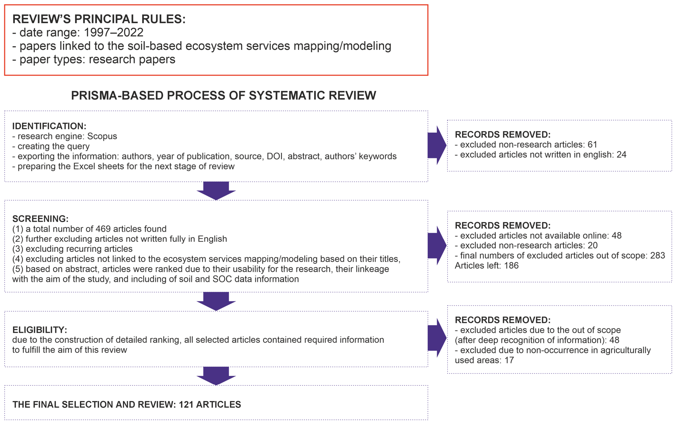
The scientific literature review was carried out based on the PRISMA 2020 rules (Figure 1) [19] to collect SES evaluation mathematical models and methods applied for agricultural soils. The preliminary assumption for the database collection considered publications issued in the English language since 1997, when the first work on ecosystem services was published [20]. The Scopus database was investigated to select research papers with the following query: TITLE-ABS-KEY (“ecosystem” AND “service*”) AND TITLE-ABS-KEY (“mapping” OR “modeling” OR “modelling” OR “model*” OR “map*”) AND TITLE-ABS-KEY (“soil*”) AND TITLE-ABS-KEY (“SOC” OR “SOM” OR “TOC” OR “organic carbon” OR “soil organic carbon” OR “soil organic matter” OR “organic matter”). The number of articles found in the first search was 469 (Supplementary Material S1), which was a satisfactory group for the screening phase. All of these papers were examined for whether they could answer the following questions: (1) “Did it include SES information?”, (2) “Did it include soil property data?”, (3) “Was it a research publication?”, and (4) “Did it include a modelling or methodological approach?”. The papers were selected based on the authors’ expert decision and received 1 point for each positively answered question. The first stage of the review process indicated that most papers (n = 375 met at least three out of the four criteria, while the number of articles which achieved a score of 1–2 points was low. The first stage of database development indicated that most papers (n = 375/469; ~80%) met 3–4 criteria, while the number of articles which achieved a score of 1–2 points was almost four times lower (n = 94/469; 20%) (Supplementary Material S1). After the screening process and careful reading of the abstract and article results, a total of 121 articles with maximum 4-point scores were selected (Figure 1).

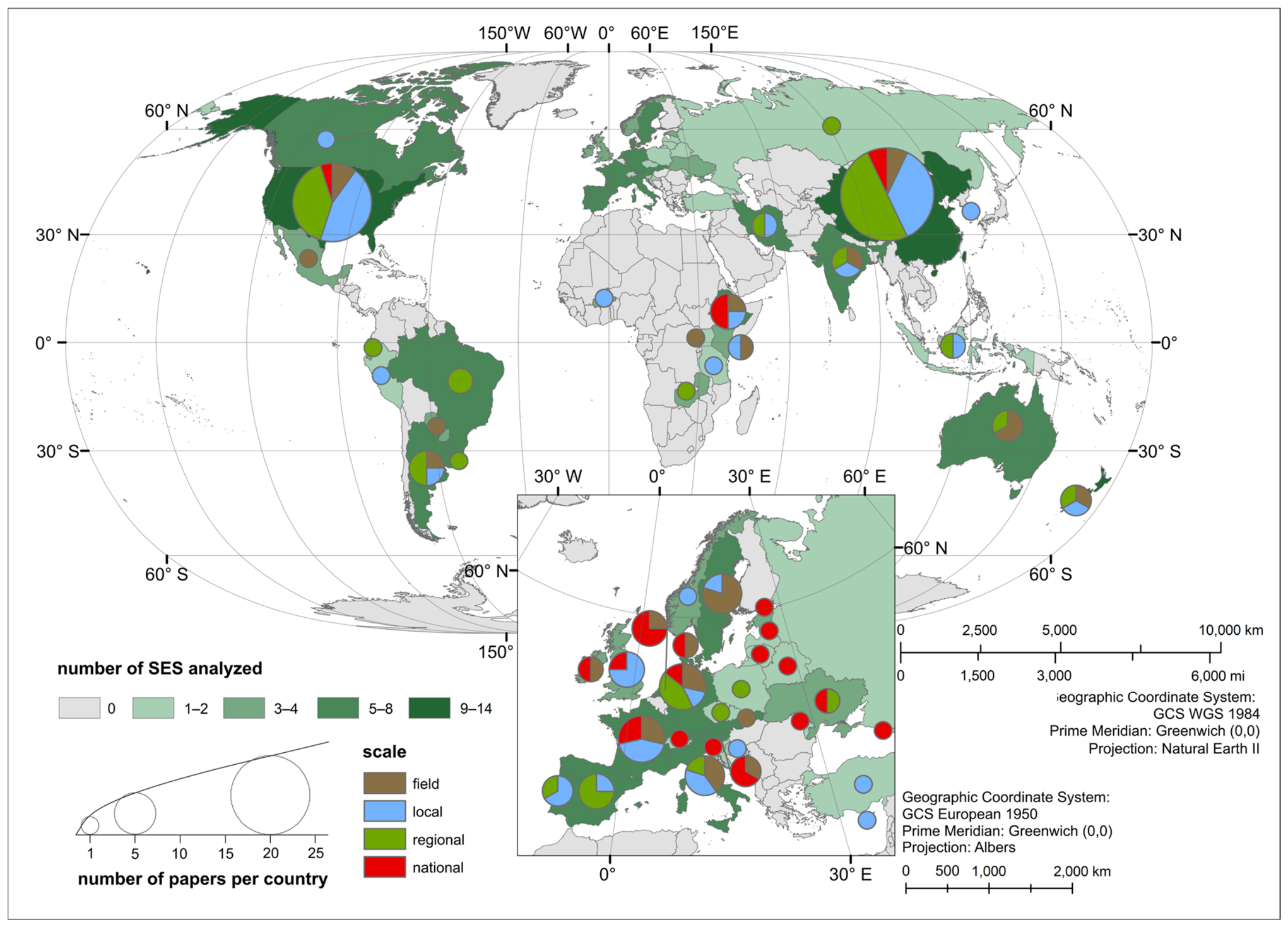
Among the selected 121 articles, 21 (17.4%) studies were performed at the field scale, 39 (32.2%) at the local scale, 38 (31.4%) at the regional scale, 13 (10.7%) at the national scale and 10 (8.3%) at the continental/global scale (Figure 2). The majority of the articles (67; 55.4%) evaluated one group of SESs, e.g., biomass production or biodiversity, while interrelations and connectivity between selected services, e.g., water holding capacity, total content of nitrogen and phosphorus and microbial activity, were recorded in 54 (44.6%) referenced papers. The SES tools were developed to evaluate predominantly regulating SESs (68; 56.2%), then provisioning SESs (31; 25.6%) and supporting SESs (22; 18.2%) (Supplementary Material S2).

2.2. SES Review General Principles

The research included two groups of SES evaluation tools: mathematical models and approximate methods. Models were categorised into the seven types according to the complexity of the applied methods. Special attention was paid to the verification and validation step, enabling comparison of the results generated by SESs with actual experimental data or observed values. Information about the validation performed was searched in selected articles. The limitations of time availability requirements, as well as resource and hardware, were not included in this review.

2.3. Grouping Factors

The studies considered nine individual SESs provided by agricultural soils: biomass production (BIOMASS), carbon sequestration potential (CSEQ), carbon stock (CSTOCKS), water retention (WATER), availability of nutrients (NUTRIENTS), emission of greenhouse gases (GHG), susceptibility to erosion (EROSION), biodiversity (BIODIVERSITY) and habitat for flora and fauna (HABITAT). In each SES, the implementation of Corg was identified, along with the role of this indicator in SES modelling. The following individual SESs were grouped into provisioning SESs: BIOMASS; regulating SESs: CSEQ, CSTOCKS, WATER, NUTRIENTS, GHH, EROSION; and supporting SESs: BIODIVERSITY, HABITAT.

2.4. SES Evaluation Methods and Models

The literature review enabled the selection of five groups (deterministic, empirical/statistical, GIS-based, mechanistic, process-based) of SES models and two groups of simple SES evaluation methods (direct measurements and proxy evaluations). The studies indicated one conceptual model originating from 2019, which illustrated the relationships between agroforestry systems, soil organic carbon sequestration, and selected soil ecosystem services, including interactions with environmental and landscape factors. This was an abstract representation of how selected individual SESs are linked to soil and environment parameters, as well as interrelated with other SESs [21]. The second recognised group of models (n = 8) were simple GIS-based approaches using simple spatial analysis and tools available in various software [15,22]. These approaches relied mainly on overlaying and combining multiple spatial data layers to identify spatial relationships and assess the distribution of SESs within a given area. As a result, the output is usually discrete data. Models based on GIS methods combine spatial data, analyses and visualisations, enabling better understanding and management of ecosystems and other resources.

The models included in the third group were process-based (n = 99). This group represents multilevel models composed of multiple parts, factors, or other submodels. They focus on the sequence of steps and mechanisms that explain processes or systems, while empirical and mechanistic models simply use statistical relationships or equations. Moreover, for each sub-part of process-based modelling, many methods and cartographic materials were used because certain model components refer to the calculation of different processes or parameters, shaping the form of the specific SES indicator [23,24,25]. Process-based models are commonly used for the evaluation of regulating SESs due to the straightforward simulation of the biochemical processes, water and SOC cycle in soil. Due to the integration of many of the subprocesses and spatial data, they also enabled the analysis based on various scenarios.

Another defined large group (n = 51) of SES empirical models used mathematical and statistical computation of environmental observations. The application of these models enables digital soil mapping to compute continuous soil maps [10,11]. They are also widely used for the prediction of soil parameters, such as SOC. Despite their scalability and multifunctionality, they strictly depend on the input data quality and availability.

The next group identified in the review were mechanistic models (n = 24), using mathematical descriptions (equations) of environmental factors or relationships between selected data and the environment [14,26,27]. They were widely used in certain situations in which the data were limited. These models were applied for the evaluation of SES-delivered maps, but with quite high uncertainty due to the complexity of soil processes. There were some inconsistencies with the literature in categorising some mechanistic models [22,28]. They could also be recognised as a part of empirical or process-based models, e.g., the K factor in the RUSLE model.

The least recognised group were the deterministic models (n = 4). Application of these tools assumed that the results were not influenced by any random element at any stage of calculation [29,30].

The studies also indicated the application of approximate evaluation methods for SESs (n = 13). These methods are effective in specific situations in which a fixed SES indicator is either not relevant or is directly linked to a certain individual SES, or the available data are not sufficient for use in the models. This approach applies meta-analysis based on the data documented in the scientific papers, which enable the factors influencing SES to be recognised [31,32].

The last group of SES qualification methods recognised in this study were direct measurements (n = 4). These methods were predominantly applied for individual fields or small regions [33,34].

3. Results

3.1. SES Evaluation Models and Methods

3.1.1. BIOMASS

BIOMASS is a provisioning SES expressing the potential of soils to produce biomass. The models applied for BIOMASS evaluation use a range of approaches, e.g., from deterministic approaches and individual-based simulations to empirical statistical methods (Supplementary Materials S2 and S3). While these models are effective in integrating key ecological drivers, they often assume linear relationships between SOC and biomass production, which may be a simple approximation of the complex soil–plant interactions, rhizosphere effects and nutrient availability in the root zone.

The Energy Budget Model [35] and NPV model [36] provide predictions for biomass and crop yields, but usually do not take into account the heterogeneity of soils and the potential influence that can change SOCs from different land uses. The empirical models [17,37,38], including RDA and PCA [38], generated a measure of statistical relationship of SOC with other biomass production under different management practices, but may have oversimplified the interaction between turnover of SOC, microbial biomass production, soil texture, and the availability of nutrients by relying mainly on statistical relationships. More complex evaluations could be completed using LCA and SEM [39,40,41], which include examining the relationship between SOC and biomass production in more than one direction.

Process-based models [12,42,43], such as DNDC [12,44,45], CENTURY [46,47,48], EPIC [49,50], and DayCent [51], have provided a more mechanistic way to evaluate how the interactions among SOC, nutrient cycles, climate factors and biomass production occur. They have also led to a better understanding of the interactions for providing biomass production and SOC dynamics, with the limitation that they are difficult to calibrate or complete using the necessary data to accurately perform the modelling [52,53]. The other limitations include difficulty of representing spatially variable SOCs [12,54], how ecosystems function in the long-term, and the importance of microbial diversity and socio-economic drivers on land management [55]. In addition, belowground biomass and SOC related to roots are not well represented by these models due to the limited field data available for their computation [38,56].

Spatially explicit models [14,57] combine high-resolution soil maps and environmental covariates to assess biomass production and SOC distribution across larger areas [26,58,59]. However, their accuracy strongly depends on the availability and quality of spatial and monitoring data, while in data-limited regions, proxy calculations are often the only possible solution [13]. Overall, BIOMASS modelling still requires better integration of nonlinear SOC interactions, spatial variability, belowground processes, and the socio-economic factors affecting land management decisions (Supplementary Material S2).

In the modelling of BIOMASS, SOC data are used as a predictor of the biomass production, reflecting its influence on the availability of nutrients, soil structure, and water retention. Empirical and statistical models assume mainly linear dependencies between SOC content and biomass indicators, which allows the use of these models for the areas of different agronomy systems (Supplementary Materials S2 and S3). These approaches successfully reflect the spatial structure, but simplify the complex and complicated system between biomass production and SOC content. On the other hand, process-based models describe more complex, multifactorial soil mechanisms. Models such as DNDC, CENTURY, EPIC, and DayCent allow the dynamic evaluation of the biomass change in different scenarios (

Table 1. Advantages and disadvantages of the identified group of models for SES BIOMASS.

Model	Model Group	SOC Usability	Advantages	Disadvantages	Validation Reported	References
Energy Budget Model; net present value model (NPV), MISCANFOR model	deterministic	- SOC data used as a model input, - SOC used as a part of the analysis	- Evaluate all energy inputs and outputs in an ecosystem, - Useful for investment and management decisions, - Helps optimise cultivation for maximum biomass and carbon storage	- Requires detailed data on energy fluxes, - Needs extensive measurements for accurate modelling, - Include economic assumptions that may not always be accurate, - Needs detailed environmental and management data	Partly	[35,36]
Heterogeneity analysis; NCCPI developed by USDA; structural equation modelling (SEM); canonical correspondence analysis (CCA); RDA model; SGS model; Life Cycle Assessment (LCA) model	empirical/statistical	- SOC as a factor affecting crop growth, biomass and yield, - SOM/SOC used as a model input, - SOC and SOM as an individual indicator for analysis, - SOC as an individual surrogate indicator for biomass production	- Models complex interactions between variables, - Identifies key drivers of biomass production and SOC sequestration, - Requires large datasets for accurate modelling, - May evaluate relationships between multiple variables	- Requires good knowledge and recognition of statistical and spatial analysis techniques, - Needs high-resolution spatial and temporal data, - Needs extensive data on various ecosystem components, - Needs comprehensive environmental and management data as well as knowledge of soil and plant processes	Yes	[17,37,38,39,41,42,60]
Set of equations	mechanistic	- SOC used to calculate NEP, - Organic topsoil data used to assess provisioning of raw materials, - SOC used to calculate biomass production (land capability)	- Simplicity of the application, - Any GIS software can be used, - Uses specific equations for detailed calculations	- Needs high-quality data for accurate results	Yes	[14,26,57,58,59]
DNDC (DeNitrification-DeComposition) model; DayCent; CENTURY model, G-Range global rangelands model; Forest-DNDC; SWAT-DayCent; EPIC model; MVS (Mean–Variance–Skewness) portfolio model; Agro-IBIS; authors’ method using remote sensing; the Austrian Climate model based on linear regression methods: Caldis vâtis as a forest growth model, CropRota model, biophysical process model EPIC, economic land-use model PASMA, BeWhere is a spatially explicit energy system model, AUSTR-IO as a dynamic multiregional input–output model; DAISY; portfolio	process-based	- SOC as an input variable, - SOC used for model initialisation, - SOM effects on the economic values of selected SESs, - SOC used to calculate linear trends or temporal changes	- Can combine many SESs, such as plant growth, soil nutrients, and water dynamics, - Can model complicated interactions and dynamics between selected parameters/SESs, - Can combine various data sources, including remote sensing, climate, land management and soil survey data, - Can model crop rotations and their impact on SOC in different scenarios, - Can model various ecosystem services and their dynamics	- For many models, there is a lack of validation and uncertainty in model parameters, - Requires detailed input data and understanding of model parameters, - Predictions may be uncertain due to the complexity of the processes, - Hardly applicable to the national, continental, or global scale	Yes	[12,43,44,45,46,47,48,49,50,51,52,53,54,55,56,61,62]
Assessment of relationships between SOC and soil quality and fertility, soil erosion, water cycle, and microbial life	proxy	- SOC used to assess trade-offs with BIOMASS-based energy sources	- relatively easy to apply and interpret	- informs only about the potential of soils to provide biomass	No	[13]

). However, their usability and uncertainty can influence the decision-making in land use and land management. A repeating problem in different types of models is the evaluation of underground biomass and SOC accumulated in the plant’s roots. This issue is mostly caused by the lack of data. Due to this fact, a majority of the methods focus on the aboveground biomass, potentially underestimating the share of the processes in soil. This is why BIOMASS modelling is highly sensitive to the data quality and scale of the input data, which indicates the need for application models that integrate SOC and its nonlinear interactions with biomass production and vegetation (Table 1).

3.1.2. CSTOCKS and CSEQ

SOC is commonly used as a key indicator for assessing carbon stocks and related SESs across diverse ecosystems. Using CSTOCKS, we evaluated the ability of soil to store the C, and CSEQ was expressed as the ability of soils to sequester C from the atmosphere. CSEQ is a more dynamic, spatiotemporal SES. Both are considered to regulate SESs. The methodologies used to model carbon stocks vary widely, including deterministic, empirical/statistical, mechanistic approaches or advanced process-based models (Supplementary Materials S2 and S3).

CSTOCKS in many models is indicated through SOC (soil organic carbon) as a principal indicator to help assess the current amount of carbon available within the soil across all types of ecosystems. The SOC data were also recognised to be used as input for both empirically-based and statistically-based models to estimate how much carbon may be sequestered, help to evaluate their quality and health, and determine what their potential for providing ecosystem services could be. SOC data can also support carbon cycling dynamics by modelling the various processes that are responsible for cycling carbon, including decomposition, mineralisation, and the relationship between carbon, vegetation, and climate variables (Table 2). Finally, SOC data are also needed as part of the validation/calibration process of models used to estimate (CSTOCK) and (CSEQ) values to validate the outputs of the simulation models.

The most precise way to determine CSTOCKS and CSEQ is through direct measurements that use field samples and laboratory analyses to provide accurate SOC-based indicators; however, direct measurements only apply over relatively small areas, and do not assist in capturing the spatial continuum of ecosystem services (Table 2; [33]; Supplementary Materials S2 and S3). Deterministic models include structured approaches to the SOC-based estimation of carbon stocks and the valuation of carbon stocks by providing a comprehensive framework through which to understand the dynamics of an SOC-based carbon stock value [28]. There are many different biotic and abiotic factors that influence the dynamic states of carbon stocks, and therefore, the ability to make informed decisions regarding land management can be improved through the use of a deterministic, SOC-based carbon stock valuation framework. The limitations of deterministic stock valuation frameworks typically relate to either their data requirements or their across-ecosystem generalisability limitations (Table 2; [28]).

All empirical/statistical models use SOC as either a predictor variable or one of the main variables influencing a CSTOCKS [63,64,65,66,67,68,69,70,71,72,73,74,75,76,77,78,79]. The following statistical methods are widely used in the determination of CSTOCKS and CSEQ: regression models, random forests, boosted regression trees, and structural equation modelling (SEM) [10,11,17,40,63,71,72,73,74,75,76,77,78,79]. Each of these statistical methods can assess uncertainty, as well as be flexible in their applicability, but they all depend on accurate data and a set of adequate statistical assumptions for their respective environments [15,64,65,66,67,68,69,70]. Many of the statistical methods encounter great difficulty in estimating complex and nonlinear SOC processes (Table 2; [10,11,17,40,63,71,72,73,74,75,76,77,78,79]).

Another type of approach is GIS-based CSTOCKS assessments, which expand the use of spatial datasets (e.g., land-use data, data obtained through remote sensing) to improve our understanding of the spatial distribution of SOC and the ecosystem service provided by SOC. The limitations of GIS-based CSTOCKS AND CSEQ estimations are similar to those of other methods, as they depend on indirect indicators and oversimplified assumptions about carbon stock systems (Table 2; [15,64,65,66]).

More complex approaches are presented in mechanistic models that represent SOC as a driver or input for carbon storage and sequestration calculations, allowing application in data-limited contexts, but that require careful calibration and often depend on simplified equations that may not fully capture SOC–CSEQ relationships (Table 2; [14,26,58,67,68,69,70]). In contrast, process-based models provide the most comprehensive representation of CSTOCKS and CSEQ by simulating SOC dynamics through biogeochemical, hydrological, and vegetation processes. Models such as DNDC, RothC, CENTURY, DayCent, EPIC, SWAT-C, CASA, InVEST, DAISY, ORCHIDEE, and others allow dynamic simulation of carbon fluxes under different land-use and climate scenarios (Table 2; [9,12,16,22,23,24,31,36,42,43,44,45,46,47,48,49,50,51,52,53,54,55,62,80,81,82,83,84,85,86,87,88,89,90,91,92,93,94,95,96,97,98]). These models can integrate multiple ecosystem functions and provide high quality process representation, but they require extensive input data and high computational resources, and are often limited in scalability and uncertainty control. However, the uncertainty associated with parameterization, especially in less-studied regions, remains a significant challenge. For instance, the use of proxy calculations or remote sensing data introduces additional complexity and potential error [13,21,32,56,89,99,100].

Across all the model groups, a persistent challenge is the strong sensitivity of CSTOCKS and CSEQ estimates to SOC data quality, spatial heterogeneity, and methodological assumptions. While process-based and empirical models can complement each other, differences in scale, input requirements, and validation practices reduce comparability across studies [16,96,99]. However, they may lack interpretability compared to simpler models and require substantial computational resources for large datasets [101,102,103]. Hybrid approaches combining measurements, statistical modelling, GIS tools, and process-based simulations are therefore increasingly applied to improve the robustness and scalability of SOC-based ecosystem service assessments (Table 2; [104,105,106,107,108]; Supplementary Material S2).

Table 2. Advantages and disadvantages of the identified group of models for SES CSTOCKS and CSEQ.

Model	Model Group	SOC Usability	Advantages	Disadvantages	Validation Reported	References
CSEQ
Direct measurements	direct measurements	- SOC stocks indicator was used to estimate CO2 sequestration and mitigation,	- low error, - small amount of time for data processing and interpretation	- does not present a continuous spatial distribution of SESs	No	[34]
Random forest, SEM, generalised linear mixed model	empirical/statistical	- SOC used to calculate C sequestration and mitigation, - SOC used to calculate SOC mineralisation and C sequestration	- availability to assess the modelling uncertainty and accuracy is very easy	- relatively long time of computation, - data must be adapted to the scale of analysis	Yes	[101,102,103]
Geospatial agricultural modelling system (GAMS), including the EPIC model	GIS-based	- SOC content as an input data for modelling	- flexibility in application, - less data required	- less precision in the SES assessment, - necessity to use indirect indicators	No	[64]
Set of equations	mechanistic	- SOC content modelled as a separate indicator, - SOC content used to calculate carbon sequestration capacity, - SOC, TC, TIC measurements used to calculate C sequestration	- does not require additional software dedicated to the individual model, - can be applied where data are limited, - does not require a specific type of data (rasters, vectors, etc.)	- for CSEQ, equations are not sufficient to evaluate the direct indicator, - requires the use of different other models to prepare data for the equation applications	Partly	[14,68,109,110,111]
InVEST; RothC; DNDC; Forest-DNDC; DayCent; SWAT-C; CASA model + improved carbon cycle process model; DAISY; GEMS; ORCHIDEE; CO2FIX	process-based	- SOC used to calculate C sequestration, - SOC used as an input for the sequestration model, - different C fractions changes used to calculate net ecosystem exchange	- wide range of model availability allows the model with the best fit to the data to be selected, - despite the high variability, provide an indicator that corresponds to the direct C sequestration indicator	- requires strong recognition and know-how of their use, - lengthy computation, - limited application at the continental and national scale, - requires more data than the other group of models	Partly	[23,25,44,45,51,52,83,85,104,105,106,107,108,112,113]
CSTOCKS
Authors’ method	deterministic	- SOC as an individual indicator	- the use of biotic and abiotic factors, providing a holistic view of SOC dynamics, - Integrates multiple drivers for carbon stocks and fluxes	- requires extensive data collection and modelling techniques, - general applicability to the other ecosystems is limited	No	[28]
Direct measurements	direct measurements	- SOC content as one of the indicators for regulating ES assessment	- provides precise SOC values through soil sampling and laboratory analysis, - straightforward approach	- requires significant time and resources for sampling and analysis, - limited to specific sampling locations, which may not represent larger areas	No	[33]
Random forest; OLS linear regression; structural equation model; bootstrapped logistic regression; boosted regression trees and robust geostatistical approaches for DSM; Gaussian mixture models; linear regression; CART model; ordinary block kriging; LCA model; multiple linear regression; ANN	empirical/statistical	- SOC content as a variable to assess SOC density or stocks, - SOC data used to calculate the SOC deficit associated with each land-use intervention, - SOC as an individual indicator	- can be applied to various datasets and scales, - useful for identifying trends and correlations, - one general model; can also be applied for smaller areas, - very applicable for SOC stocks, - some methods are effective in detecting complex relationships in SOC data, - simple regression models are straightforward and easy to implement, - many models can handle nonlinear relationships	- highly dependent on the quality and quantity of available data, - relies on statistical assumptions that may cause a significant predictive error, - advanced machine learning models can be difficult to implement and interpret, - many of the models tend to overfit, especially with small datasets, - the final performance and detection of complex SOC relationships and cycles depend on the applied method: simple regression is easy to interpret and does not require a long time for computation, advanced models can handle multiple predictors and interactions, but require specialistic knowledge and a long time for computation	Yes	[10,11,17,40,63,71,72,73,74,75,76,77,78,79]
Global soc–climate interactions model; GIS-based calculations for mand use classes; estimating ESS based on land cover classes; GAMS including EPIC model	GIS-based	- SOC content as an input data/ indicator for modelling	- can easily combine various data sources, including remote sensing and land-use data, - flexibility in application - less data required	- predictions may be uncertain, - less precision in the SES assessment, - necessity to use indirect indicators	No	[15,64,65,66]
Set of indicators	mechanistic	- SOC content to assess C storage and cycling, - SOC content used to calculate SOC stocks, - SOM as soil parameters used in modelling	- commonly used for SOC stock calculation, - easy to apply with any GIS software	- needs extensive data on selected components	Partly	[26,58,67,68,69,70]
DNDC model; RothC; InVEST model, PLUS model; CASA model; InVEST; DayCent; PnET-BGC; TOA-MD; APSIM; CENTURY; ECOSER protocol; Ag-EcoSOpt tool; Forest-DNDC; SWAT-DayCent; EPIC; G-Range based on CENTURY; CARBOSAF; Mean–Variance–Skewness portfolio model; Agro-IBIS; LPJ-WHyMe and LPX; MOSES-LSH; the Basin Characterisation Model; Yasso07 soil carbon model; DAISY; biogeochemical model ForSAFE; WaNuLCAS; net present value model, MISCANFOR model; Portfolio Model; TEM, and Biome-BGC	process-based	- SOC content as a model variable, - SOC data used for soil organic carbon pool simulations, - SOC as an input data for modelling, - SOC data used for the calculation of spatiotemporal changes in carbon storage, - different C fraction changes used to calculate net ecosystem exchange, - SOM effects on the economic values of selected ES	- provides effective prediction of SOC changes under different scenarios, - can be adapted to different environmental contexts, - can model multiple SESs in one process; - can handle modelling multiple dimensions of SOC dynamics, - can simulate short-time carbon fluxes, - can be applied at any scale	- requires extensive data and modelling techniques, - predictions may be uncertain due to the complexity of the processes, - requires detailed knowledge of the models and their applications, - needs high-quality data for accurate results, - needs very good computational resources, - high complexity: requires detailed input data and understanding of model parameters, - may require additional software to use	Yes	[9,12,16,22,24,31,36,42,43,44,45,46,47,49,50,52,53,54,55,62,80,81,82,83,84,85,86,87,88,89,90,91,92,93,94,95,96,97,98]
Spatially explicit pressure analysis; authors’ method using remote sensing; general ecosystem service model; assessment of relationships between SOC and soil quality and fertility; review of the existing data	proxy	- SOC used to assess SES capacity or C storage potential	- combines various data sources, including remote sensing and soil surveys, - provides a structured approach to SOC estimation, - easy to implement and interpret	- needs extensive data for accurate assessments, - provides basic insights into SOC trends and patterns, - relies on assumptions that may not always be valid	Partly	[13,21,32,56,95,96]

Table 2. Advantages and disadvantages of the identified group of models for SES CSTOCKS and CSEQ.

Model	Model Group	SOC Usability	Advantages	Disadvantages	Validation Reported	References
CSEQ
Direct measurements	direct measurements	- SOC stocks indicator was used to estimate CO2 sequestration and mitigation,	- low error, - small amount of time for data processing and interpretation	- does not present a continuous spatial distribution of SESs	No	[34]
Random forest, SEM, generalised linear mixed model	empirical/statistical	- SOC used to calculate C sequestration and mitigation, - SOC used to calculate SOC mineralisation and C sequestration	- availability to assess the modelling uncertainty and accuracy is very easy	- relatively long time of computation, - data must be adapted to the scale of analysis	Yes	[101,102,103]
Geospatial agricultural modelling system (GAMS), including the EPIC model	GIS-based	- SOC content as an input data for modelling	- flexibility in application, - less data required	- less precision in the SES assessment, - necessity to use indirect indicators	No	[64]
Set of equations	mechanistic	- SOC content modelled as a separate indicator, - SOC content used to calculate carbon sequestration capacity, - SOC, TC, TIC measurements used to calculate C sequestration	- does not require additional software dedicated to the individual model, - can be applied where data are limited, - does not require a specific type of data (rasters, vectors, etc.)	- for CSEQ, equations are not sufficient to evaluate the direct indicator, - requires the use of different other models to prepare data for the equation applications	Partly	[14,68,109,110,111]
InVEST; RothC; DNDC; Forest-DNDC; DayCent; SWAT-C; CASA model + improved carbon cycle process model; DAISY; GEMS; ORCHIDEE; CO2FIX	process-based	- SOC used to calculate C sequestration, - SOC used as an input for the sequestration model, - different C fractions changes used to calculate net ecosystem exchange	- wide range of model availability allows the model with the best fit to the data to be selected, - despite the high variability, provide an indicator that corresponds to the direct C sequestration indicator	- requires strong recognition and know-how of their use, - lengthy computation, - limited application at the continental and national scale, - requires more data than the other group of models	Partly	[23,25,44,45,51,52,83,85,104,105,106,107,108,112,113]
CSTOCKS
Authors’ method	deterministic	- SOC as an individual indicator	- the use of biotic and abiotic factors, providing a holistic view of SOC dynamics, - Integrates multiple drivers for carbon stocks and fluxes	- requires extensive data collection and modelling techniques, - general applicability to the other ecosystems is limited	No	[28]
Direct measurements	direct measurements	- SOC content as one of the indicators for regulating ES assessment	- provides precise SOC values through soil sampling and laboratory analysis, - straightforward approach	- requires significant time and resources for sampling and analysis, - limited to specific sampling locations, which may not represent larger areas	No	[33]
Random forest; OLS linear regression; structural equation model; bootstrapped logistic regression; boosted regression trees and robust geostatistical approaches for DSM; Gaussian mixture models; linear regression; CART model; ordinary block kriging; LCA model; multiple linear regression; ANN	empirical/statistical	- SOC content as a variable to assess SOC density or stocks, - SOC data used to calculate the SOC deficit associated with each land-use intervention, - SOC as an individual indicator	- can be applied to various datasets and scales, - useful for identifying trends and correlations, - one general model; can also be applied for smaller areas, - very applicable for SOC stocks, - some methods are effective in detecting complex relationships in SOC data, - simple regression models are straightforward and easy to implement, - many models can handle nonlinear relationships	- highly dependent on the quality and quantity of available data, - relies on statistical assumptions that may cause a significant predictive error, - advanced machine learning models can be difficult to implement and interpret, - many of the models tend to overfit, especially with small datasets, - the final performance and detection of complex SOC relationships and cycles depend on the applied method: simple regression is easy to interpret and does not require a long time for computation, advanced models can handle multiple predictors and interactions, but require specialistic knowledge and a long time for computation	Yes	[10,11,17,40,63,71,72,73,74,75,76,77,78,79]
Global soc–climate interactions model; GIS-based calculations for mand use classes; estimating ESS based on land cover classes; GAMS including EPIC model	GIS-based	- SOC content as an input data/ indicator for modelling	- can easily combine various data sources, including remote sensing and land-use data, - flexibility in application - less data required	- predictions may be uncertain, - less precision in the SES assessment, - necessity to use indirect indicators	No	[15,64,65,66]
Set of indicators	mechanistic	- SOC content to assess C storage and cycling, - SOC content used to calculate SOC stocks, - SOM as soil parameters used in modelling	- commonly used for SOC stock calculation, - easy to apply with any GIS software	- needs extensive data on selected components	Partly	[26,58,67,68,69,70]
DNDC model; RothC; InVEST model, PLUS model; CASA model; InVEST; DayCent; PnET-BGC; TOA-MD; APSIM; CENTURY; ECOSER protocol; Ag-EcoSOpt tool; Forest-DNDC; SWAT-DayCent; EPIC; G-Range based on CENTURY; CARBOSAF; Mean–Variance–Skewness portfolio model; Agro-IBIS; LPJ-WHyMe and LPX; MOSES-LSH; the Basin Characterisation Model; Yasso07 soil carbon model; DAISY; biogeochemical model ForSAFE; WaNuLCAS; net present value model, MISCANFOR model; Portfolio Model; TEM, and Biome-BGC	process-based	- SOC content as a model variable, - SOC data used for soil organic carbon pool simulations, - SOC as an input data for modelling, - SOC data used for the calculation of spatiotemporal changes in carbon storage, - different C fraction changes used to calculate net ecosystem exchange, - SOM effects on the economic values of selected ES	- provides effective prediction of SOC changes under different scenarios, - can be adapted to different environmental contexts, - can model multiple SESs in one process; - can handle modelling multiple dimensions of SOC dynamics, - can simulate short-time carbon fluxes, - can be applied at any scale	- requires extensive data and modelling techniques, - predictions may be uncertain due to the complexity of the processes, - requires detailed knowledge of the models and their applications, - needs high-quality data for accurate results, - needs very good computational resources, - high complexity: requires detailed input data and understanding of model parameters, - may require additional software to use	Yes	[9,12,16,22,24,31,36,42,43,44,45,46,47,49,50,52,53,54,55,62,80,81,82,83,84,85,86,87,88,89,90,91,92,93,94,95,96,97,98]
Spatially explicit pressure analysis; authors’ method using remote sensing; general ecosystem service model; assessment of relationships between SOC and soil quality and fertility; review of the existing data	proxy	- SOC used to assess SES capacity or C storage potential	- combines various data sources, including remote sensing and soil surveys, - provides a structured approach to SOC estimation, - easy to implement and interpret	- needs extensive data for accurate assessments, - provides basic insights into SOC trends and patterns, - relies on assumptions that may not always be valid	Partly	[13,21,32,56,95,96]

3.1.3. WATER

Water circulation and production are critical components of ecosystem services and influence agricultural productivity, water quality and carbon sequestration. This regulating SES is directly linked to the availability of soil components to support the water cycle and water retention. Understanding these processes requires detailed models that can simulate the complex interactions between soil water and vegetation.

SOC data are used in WATER modelling primarily for their role as a proxy for soil structure, infiltration capacity, and water retention, all of which directly affect water supply and yield. In general, SOC features as an input variable in process-based models such as InVEST, SWAT, and STICS to simulate water balance, runoff, evapotranspiration, and hydrologic processes on an area-wide scale (Table 3). Within these models, SOC is used to better assess interactions between soil and vegetation that function to influence seasonal and annual volumes of surface water generated. Additionally, SOC is used as an indirect means to represent the effects of sediment transfer and nutrient cycling within integrated models such as SWAT-DayCent (Table 3), as well as to calibrate and validate hydrological models to provide better estimates of water provision services under various land-use and climatic conditions.

The most common indicator was the water yield, which can be successfully evaluated through process-based models, such as the InVEST model (Supplementary Materials S2 and S3). The water yield component estimates annual water yield based on water balance principles. However, it is data-intensive, requiring extensive input data, including climate and land use, and involves advanced and extensive modelling techniques. The InVEST model can integrate multiple ecosystem services for comprehensive analysis, but it also requires high-quality data and involves complex modelling techniques. Moreover, the InVEST model can assess seasonal water yield, estimating both annual and seasonal water yields and providing detailed spatial analysis (Table 3) [18,30,86,105,114]. Highly important and widely used is the SWAT—Soil and Water Assessment Tool—for modelling water sediment and agricultural chemical movement in watersheds. It is versatile and applicable to various land management practices, but it requires detailed input data and understanding of model parameters and needs extensive validation with field data (Supplementary Materials S2 and S3, Table 3, [115]). A modification of the SWAT—the hydro-biogeochemical model SWAT-DayCent—combines hydrological and biogeochemical modelling, providing comprehensive modelling of water and nutrient dynamics, but it requires detailed knowledge of the models and data for accurate results (Table 3, [54]). Another model is the ES trade-off degree (ESTD) model, which analyses multiple ecosystem services for comprehensive analysis and is effective in predicting trade-offs among ecosystem services. It requires extensive data and advanced modelling techniques, but also needs field data for validation (Table 3, [86]). For this SES, we also identified the agricultural production systems sIMulator APSIM, DAISY, and ERGOM. They can model various agricultural production systems and are effective in predicting water and nutrient dynamics. The ERGOM model is suitable for marine and coastal ecosystems. The MONERIS model is able to evaluate nutrient emissions from various sources and nutrient dynamics. It requires extensive data and sophisticated modelling techniques and needs thorough validation with field data. The STICS model is a comprehensive model of crop growth and soil processes and is effective in predicting water and nutrient dynamics. All four models require detailed and high-quality data as well as a validation process (Table 3, [52,116,117]). A highly recommended model is STICS. It effectively models crop growth and soil processes, but also simulates water and nutrient dynamics. STICS requires extensive data and know-how on modelling techniques (Table 3, [118]). These models provide valuable insights into water circulation and production using SOC data, but they also cause many challenges related to data requirements and validation.

Table 3. Advantages and disadvantages of the identified group of models for SES WATER.

Model	Model Group	SOC Usability	Advantages	Disadvantages	Validation Reported	References
Direct measurements	direct measurements	- SOC content as one of the indicators for regulating ES assessment	- provides precise values through soil sampling and laboratory analysis - straightforward approach	- requires significant time and resources for sampling and analysis, - limited to specific sampling locations, which may not represent larger areas, - requires a lot of measurements to evaluate dynamics	No	[33]
InVEST model; SWAT; Seasonal Water Yield Model, ES trade-off degree model; SWAT-DayCent; DAISY; ERGOM; MONERIS; STICS	process-based	- SOC and SOM as input data for modelling	- many models are open-source and accessible, - possible to apply to various land management practices, - can simulate complicated water processes such as water, sediment, and agricultural chemical movement in watersheds, - are able to estimate both annual and seasonal water yields, - can be highly applicable in predicting trade-offs among ecosystem services	- requires extensive input data, including climate and land use, - needs high-quality, extensive data for accurate results, - requires time to understand the process of modelling, - needs extensive validation	Yes	[18,30,52,54,86,105,114,115,116,118]
APSIM	proxy	- SOC as an impact on nitrogen cycling and soil physical properties	- the model requires extensive data	- does not provide detailed information about water provision or the water cycle	No	[117]

Table 3. Advantages and disadvantages of the identified group of models for SES WATER.

Model	Model Group	SOC Usability	Advantages	Disadvantages	Validation Reported	References
Direct measurements	direct measurements	- SOC content as one of the indicators for regulating ES assessment	- provides precise values through soil sampling and laboratory analysis - straightforward approach	- requires significant time and resources for sampling and analysis, - limited to specific sampling locations, which may not represent larger areas, - requires a lot of measurements to evaluate dynamics	No	[33]
InVEST model; SWAT; Seasonal Water Yield Model, ES trade-off degree model; SWAT-DayCent; DAISY; ERGOM; MONERIS; STICS	process-based	- SOC and SOM as input data for modelling	- many models are open-source and accessible, - possible to apply to various land management practices, - can simulate complicated water processes such as water, sediment, and agricultural chemical movement in watersheds, - are able to estimate both annual and seasonal water yields, - can be highly applicable in predicting trade-offs among ecosystem services	- requires extensive input data, including climate and land use, - needs high-quality, extensive data for accurate results, - requires time to understand the process of modelling, - needs extensive validation	Yes	[18,30,52,54,86,105,114,115,116,118]
APSIM	proxy	- SOC as an impact on nitrogen cycling and soil physical properties	- the model requires extensive data	- does not provide detailed information about water provision or the water cycle	No	[117]

3.1.4. NUTRIENTS

Except for SOC, SOM, and the water cycle, an important soil variable is nutrient content and provision. Nutrient provision is a critical component of ecosystem services, influencing agricultural productivity, soil health and carbon sequestration by presenting the potential and the state of the soil for storing the nutrients and providing them to plants. Understanding these processes requires robust models that can simulate the complex interactions between soil nutrients and vegetation (Supplementary Materials S2 and S3). Among them, SOC plays a crucial role, not only as a source of nutrients in soils, but also as a driver of their transformation and the increase in soil sorption [3,5,6,10]. SOC data are mostly used as key input and proxy variables for estimating nutrient availability, specifically nitrogen and phosphorus cycling, and for determining the soil fertility level (Table 4).

Many models were found to assess these constituents, such as multiple linear regression analysis (MLRA), a statistical method used to understand the relationship between multiple independent and dependent variables. It is straightforward and widely used but can be limited by its assumption of linearity and the need for large datasets (Table 4, [102]). Regarding multifunctional models, structural equation modelling (SEM), being a multivariate statistical analysis technique, is used to analyse structural relationships (Table 4, [102,119,120,121]). As a supplement, the stepwise approach based on the ES cascade model is a good approach that adds or removes variables based on their statistical significance. It is useful for simplifying models but can sometimes lead to overfitting (Table 4, [17]). For the multifactorial analysis, PCA (Principal Component Analysis) was used. This method is applied to reduce the dimensions of datasets, increasing interpretability while minimising information loss. It is effective for handling large datasets but can be complex to implement (Table 4, [122]). GIS models are used to analyse spatial and geographic data. They can be useful for visualising and analysing spatial relationships but require specialised software and connecting many factors of nutrient provision (Table 4, [123]). Strong tools are the process-based models, such as the DNDC model, used to simulate the carbon and nitrogen cycle in agroecosystems. This model is comprehensive and dynamic but requires detailed input data (Table 4, [12,23]). The Forest-DNDC model is a variant tailored for forest ecosystems, incorporating specific processes relevant to forest biogeochemistry (Table 4, [44]). Another approach is the EPIC Environmental Policy Integrated Climate model with the N leaching module used to simulate nitrogen leaching in agricultural systems. It is effective for policy analysis but requires extensive data and calibration (Table 4, [50]). We also identified the CENTURY, TEM Terrestrial Ecosystem Model, and Biome-BGC Biogeochemical Cycles. They are ecosystem models used to simulate carbon, nitrogen and water cycles. Together, they are comprehensive but require detailed input data and understanding of ecosystem processes (Table 4, [9]). Lastly, the Agricultural Production Systems sIMulator APSIM is used to model agricultural systems, allowing the proxy prediction of water and nutrient dynamics (Table 4, [117]). Within these models, SOC is included as a variable or an element of the nutrient cycle [120] or is included as an indicator directly in the modelling of the processes [17,33,102,117,120,124].

Table 4. Advantages and disadvantages of the identified group of models for SES NUTRIENTS.

Model	Model Group	SOC Usability	Advantages	Disadvantages	Validation Reported	References
Author’s model; regression analysis, structural equation modelling (SEM); canonical correspondence analysis (CCA); linear mixed effects models; PCA	empirical/statistical	- SOC as one of the variables in modelling, - SOC as a surrogate indicator for nutrient cycling and retention	- simple regression analyses are easy to implement and interpret, - can measure complex relationships between variables, - simplifies large datasets while retaining important information,	- needs large datasets for high accuracy and spatial predictions, - some methods may not capture nonlinear relationships, - can sometimes exclude important variables	Yes	[17,33,71,102,119,120,121,122,124]
Set of spatial and geostatistical tools	GIS-based	- SOM as an indicator for soil fertility maintenance	- sufficient in visualising and analysing spatial relationships, - combines various data sources for comprehensive analysis, - easy to modify and adapt to the available data	- needs high-quality spatial data	No	[123]
Set of equations	mechanistic	- depth of humus horizon used to evaluate sorption potential, - C/N ratio used to calculate N mineralisation rate	- simplicity of the application, - Any GIS software can be used, - uses specific equations for detailed calculations	- needs high-quality data for accurate results	No	[70,125]
DNDC (DeNitrification-DeComposition) model; Forest-DNDC; EPIC model: N leaching module; CENTURY, TEM, and Biome-BGC	process-based	- simulation of the carbon cycle as a model input, - SOC as one of the variables in modelling	- applicable to various ecosystems, - combines various data sources for comprehensive analysis	- requires detailed input data and understanding of parameters, - for better accuracy, needs extensive field validation, - predictions may be uncertain due to process complexity or simplification	Yes	[9,12,23,44,50]
APSIM	proxy	- SOC as an impact on nitrogen cycling and soil physical properties	- the model requires extensive data	- does not provide detailed information about the nutrient cycle	No	[117]

Table 4. Advantages and disadvantages of the identified group of models for SES NUTRIENTS.

Model	Model Group	SOC Usability	Advantages	Disadvantages	Validation Reported	References
Author’s model; regression analysis, structural equation modelling (SEM); canonical correspondence analysis (CCA); linear mixed effects models; PCA	empirical/statistical	- SOC as one of the variables in modelling, - SOC as a surrogate indicator for nutrient cycling and retention	- simple regression analyses are easy to implement and interpret, - can measure complex relationships between variables, - simplifies large datasets while retaining important information,	- needs large datasets for high accuracy and spatial predictions, - some methods may not capture nonlinear relationships, - can sometimes exclude important variables	Yes	[17,33,71,102,119,120,121,122,124]
Set of spatial and geostatistical tools	GIS-based	- SOM as an indicator for soil fertility maintenance	- sufficient in visualising and analysing spatial relationships, - combines various data sources for comprehensive analysis, - easy to modify and adapt to the available data	- needs high-quality spatial data	No	[123]
Set of equations	mechanistic	- depth of humus horizon used to evaluate sorption potential, - C/N ratio used to calculate N mineralisation rate	- simplicity of the application, - Any GIS software can be used, - uses specific equations for detailed calculations	- needs high-quality data for accurate results	No	[70,125]
DNDC (DeNitrification-DeComposition) model; Forest-DNDC; EPIC model: N leaching module; CENTURY, TEM, and Biome-BGC	process-based	- simulation of the carbon cycle as a model input, - SOC as one of the variables in modelling	- applicable to various ecosystems, - combines various data sources for comprehensive analysis	- requires detailed input data and understanding of parameters, - for better accuracy, needs extensive field validation, - predictions may be uncertain due to process complexity or simplification	Yes	[9,12,23,44,50]
APSIM	proxy	- SOC as an impact on nitrogen cycling and soil physical properties	- the model requires extensive data	- does not provide detailed information about the nutrient cycle	No	[117]

3.1.5. BIODIVERSITY

Biodiversity is a challenging problem to map and analyse, due to the soil complexity in biological properties. SOC plays a crucial role in the evaluation of biodiversity due to it being the main source of energy and nutrition for soil organisms. Higher SOC content supports higher microbial activity, species richness and functional diversity, while a SOC decrease will reduce the number of organisms [67,111]. SOC information was used mostly as a key environmental predictor in modelling biodiversity through determining habitat quality, soil fertility, and ecosystem function. These data are also included in both empirical and statistical models (e.g., Shannon Index method; SEM; GLM; CCA), quantifying the relationships between soil carbon and species diversity patterns. In GIS-based or proxy methods, SOC-related variables (e.g., total carbon stocks or SOM) are used in evaluating the impacts of land use on biodiversity and in assisting with the spatially explicit mapping of biodiversity indicators in landscapes (

Table 5. Advantages and disadvantages of the identified group of models for SES BIODIVERSITY.

Model	Model Group	SOC Usability	Advantages	Disadvantages	Validation Reported	References
Direct measurements	direct measurements	- SOC content as a one of the indicators for regulating ES assessment (ES diversity)	- provides precise values through soil sampling and laboratory analysis - straightforward approach	- requires significant time and resources for sampling and analysis - limited to specific sampling locations, which may not represent larger areas - requires a lot of measurements to evaluate dynamics	No	[33]
Shannon indices, SEM; linear mixed effect model; CCA Ordinations, CSR distribution model; GLMs; stepwise multiple regression and other statistics; Shannon–Weaver Index; Faith’s Index; GWR plus Shannon Diversity Index; multiple linear regression	empirical/statistical	- SOC as one of the environmental factors/variables, - SOC as an individual indicator and correlation factor with biodiversity	- provides a wide range of metrics that inform assessments of diversity, - many models can analyse complex relationships and interactions, - DSM approach increases the accuracy of biodiversity models	- simple indices that can struggle to analyse species interactions, - requires large sample sizes, detailed species and environmental data, - simple linear models that can be sensitive to multicollinearity	Yes	[17,41,67,73,121,124,126,127,128,129,130,131,132]
GIS-based calculations for land-use classes	GIS-based	- total carbon storage per tree species as an environmental factor	- easy to apply, - useful for understanding land-use impacts on SOC and biodiversity	- requires accurate data, - can be too complex or too simple to implement	No	[65]
set of equations	mechanistic	- not directly	- simplicity of application, - any GIS software can be used, - uses specific equations for detailed calculations	- needs high-quality data for accurate results	No	[111]
Decision Model (DEX Model)	proxy	- SOM used as an attribute in grassland and cropland models of soil biodiversity	- evaluates multiple criteria and indicators	- qualitative results may lack precision, - requires expert knowledge to develop criteria and indicators	Yes	[133]

).

Biodiversity models are essential for understanding and predicting the impacts of various factors on ecosystems as well as soil health and fertility. They are labour-intensive but offer high precision and reliability (Supplementary Materials S2 and S3). Using these data, we can apply landscape metric measures. The Shannon Index is a measure of species diversity in a bigger community. It analyses both the abundance and evenness of species present in soils. Combined with SOC data, it helps in understanding the relationship between soil health and biodiversity (Table 5, [126]). In the next step, SEM can enrich the studies. This method is particularly useful in biodiversity studies as it can incorporate multiple variables and their interactions. SEM can be used to model the direct and indirect effects of SOC on biodiversity. Moreover, it does not require high-quality spatial data (Table 5, [41,121,126]). Linear mixed effect models are suitable for biodiversity studies involving SOC data as they can account for both fixed and random effects, providing a more comprehensive understanding of the factors influencing biodiversity (Table 5, [127,128]). One of the multidimensional studies is CCA—an ordination method used to understand the relationships between biological assemblages and environmental variables. By incorporating SOC data, CCA can help identify the key environmental gradients affecting biodiversity (Table 5, [17,129]). For a spatial prediction, a DSM approach was applied. It uses field data with spatial and soil covariates. This approach can enhance the accuracy of biodiversity models by providing detailed maps. However, due to data accessibility, it is rarely applied (Table 5, [130]). Another statistical approach is the stepwise multiple regression used to identify the most significant predictors of biodiversity from a set of variables. This method, along with other statistical techniques such as the Shannon Diversity Index, can be used to analyse the relationship between SOC and biodiversity (Table 5, [131]). GWR as a DSM algorithm can be used to explore the spatial variation in the relationship between SOC and biodiversity, as well as to prepare prediction maps (Table 5, [132]). Lastly, the DEX was identified as a qualitative multi-criteria decision analysis method. It can be used to evaluate the impact of different management practices on SOC and biodiversity by integrating various indicators and criteria (Table 5, [133]). Biodiversity models using SOC data are crucial for understanding the complex interactions within ecosystems.

3.1.6. HABITAT

Habitat provision and support models are crucial in understanding, managing, and protecting ecosystems. Calzolari et al. [14] used a set of equations and hotspot analysis to identify areas with significant SOC levels. SOC and bulk density were used to calculate the land capability map and potential habitat for soil organisms. This approach involves direct measurements of SOC and the application of statistical models to detect spatial patterns and hotspots of habitat condition. Hotspot analysis helps in identifying critical areas that require conservation or management interventions. However, this process is resource-intensive, requiring extensive fieldwork and laboratory analysis, making it time-consuming and costly (

Table 6. Advantages and disadvantages of the identified group of models for SES HABITAT.

Model	Model Group	SOC Usability	Advantages	Disadvantages	Validation Reported	References
The Basin Characterisation Model	empirical/statistical	- SOC data used to generate a map of ecologically active stocks of soil organic carbon	- useful for forecasting changes in SOC under different environmental scenarios, aiding in long-term habitat management	- requires extensive datasets, including climate, hydrology, and land-use information, - the high complexity of the model can make it difficult to implement and interpret	No	[100]
Set of equations and hotspot analysis	mechanistic	- SOC used to evaluate land capability map, potential habitat for soil organisms	- hotspot analysis helps in identifying critical areas that require conservation or management interventions, - relatively easy to apply with any GIS software, - model is replicable and can be applied to other areas	- the process requires extensive fieldwork and laboratory analysis, making it time-consuming and costly (due to the specific area), - developing and validating the model can be challenging and time-consuming, requiring significant expertise and resources	No	[14]
Decision Model (DEX Model)	proxy	- SOM used as an attribute in grassland and cropland models of soil biodiversity and habitat provision	- useful in scenarios where quantitative data are limited or uncertain	- the model relies on expert judgment, which can introduce bias and variability in the results	Yes	[133]

). The Decision Model (DEX Model) assesses soil functions, including biodiversity and habitat provisioning [133]. This model integrates multiple criteria and indicators to evaluate soil quality and its capacity to support biodiversity. In this model, SOM was used as an attribute in grassland and cropland models of habitat provision. The DEX Model incorporates various indicators and criteria, making it suitable for complex environmental decisions. It is particularly useful in scenarios where quantitative data are limited or uncertain, providing an assessment of soil functions. However, the model relies on expert judgment, which can introduce bias and variability in the results (Table 6). On the other hand, the Basin Characterisation Model was applied to understand SOC dynamics at the basin scale [100]. This model integrates hydrological and climatic data to predict SOC distribution and its impact on habitat quality. The Basin Characterisation Model provides a detailed understanding of SOC dynamics by incorporating various environmental factors. It is useful for forecasting changes in SOC under different environmental scenarios, aiding in long-term habitat management. However, the model is data-intensive, requiring extensive datasets, including climate, hydrology, and land-use information, which can be challenging to obtain. The high complexity of the model can also make it difficult to implement and interpret, requiring specialised knowledge and tools (Supplementary Materials S2 and S3, Table 3).

3.1.7. GHG

Another environmentally significant SES identified was the greenhouse gas (GHG) emissions and climate regulation. This supporting SES assesses the fluxes of selected GHG, such as CO₂, CH₄, NH₄, and NO₃, between the soil and atmosphere. In GHG SES evaluation, SOC data are used widely to model soil carbon status and determine (predict) the interaction between GHG emissions or fluxes and soil carbon. Empirical/statistical approaches such as boosted regression trees, SEM, or LCA also use SOC data to describe, explain, and predict nonlinear relationships between soil properties and CO₂, CH₄, and N₂O emissions. SOC is also used as a primary input parameter to simulate carbon/nitrogen cycling, estimate net ecosystem exchange under differing management practices, and provide input to GHG modelling through atmospheric processes (

Table 7. Advantages and disadvantages of identified group of models for SES GHG.

Model	Model Group	SOC Usability	Advantages	Disadvantages	Validation Reported	References
Empirically validated boosted regression tree; LCA; ANN	empirical/statistical	- SOM used as a covariate for modelling, - SOC used for the evaluation of the SOC relative changes to assess climate regulation potential	- combines multiple models to reduce error and improve predictions, - can evaluate complex, nonlinear relationships between variables, - considers all stages of a product’s life cycle, providing a holistic view of environmental impacts	- requires significant computational resources, - model is complex, hence the interpretation can be challenging, - requires extensive data collection for accurate assessments	Yes	[40,89,134]
Matrix method, estimating SES based on land cover classes, the Map Comparison Statistic	GIS-based	- SOC used as a quantitative indicator to map global climate regulation potential	- can integrate various types of environmental data for comprehensive analyses, - easy to apply, - suitable for both observation and experimental data	- requires accurate and high-resolution spatial data	No	[15]
Set of equations	mechanistic	- SOC data used to calculate cumulative soil respiration, C biomass, - SOC used directly in the model as a variable	- straightforward to implement and interpret, - any GIS software can be used, - uses specific equations for detailed calculations	- needs high-quality data for accurate results, - may oversimplify the complex process of climate regulation	Partly	[125,135]
DayCent; Ag-EcoSOpt tool; Forest-DNDC; DNDC; (EPX) model	process-based	- SOC as model input parameter, - different C fractions changes used to calculate net ecosystem exchange and GHG fluxes	- provides detailed daily simulations of carbon and nitrogen cycles, - useful for forecasting the impacts of different management practices, - can be adapted to different ecosystems and management practices	- requires extensive data and expertise to implement, - high computational demands for running simulations, - integration of multiple models can be challenging	Yes	[23,44,51,89,136]
LPJ-WHyMe and LPX model, part of ORCHIDEE, the MOSES-LSH, the McGill Wetland Model, climate model, GISS GCM model for methane emissions	proxy	- SOC as an input data for modelling	- useful for forecasting the impacts of different management practices - incorporates SOC data for comprehensive climate regulation analysis	- high computational demands for running simulations, - requires extensive data and expertise to implement, - do not include direct indicators for the GHG emissions	No	[31]

).

There is a wide range of statistical techniques, such as boosted regression trees, which can be used to estimate GHG emissions using SOC data. These techniques have been thoroughly examined and shown to produce accurate estimates of GHG emissions (Table 7) as well as to model the complex, and often nonlinear, relationships between SOC and GHG emissions [134]. Life cycle analysis models that incorporate SOC data allow for the quantification of GHG emissions over the life of a product or system, as well as provide a more holistic assessment of the carbon cycle and ecosystem models (Table 7; [40]). On the other hand, SEM models assess GHG emission, SOC, and environmental interaction and require large datasets, and may have higher sensitivity to the specification and complexity of model interpretation. Therefore, we recognised alternative models, such as GIS-based mapping of SOC distribution and related GHG emissions that allow for identifying spatial hotspots for SOC and GHG emissions, but the performance of GIS-based mapping methods is highly dependent on the quality and resolution of data [15]. Another approach is a wide range of mechanistic models representing the relationships between SOC and GHG emissions using various equations, and, as such, are easier to apply than complex (statistical) methods; however, they can oversimplify the model of the ecologically complex process between SOC and GHG emissions and depend on reliable input data (Table 7; [125,135]). Additionally, many process-based models were recognised, such as DayCent, generating carbon and nitrogen flux estimates (GHG emissions) based on SOC (static organic carbon), by providing a high level of detail regarding processes that take place throughout the day. DayCent is limited to the local scale but provides accurate and highly detailed data on many processes that affect carbon cycling (Table 7; [51]). Many of the integrated process models, with the exception of Ag-EcoSOpt, integrate multiple different models and improve predictive capability and complexity, and allow scenario analysis to be performed (Table 7; [23,44,89,136]); however, they require more data for calibration and increase the complexity of process models when using an integrated approach. Incorporating SOC into vegetation-based models, as applied in large-scale climate and vegetation models such as LPJ-WHyMe, LPX, the McGill Wetland Model, and GISS GCM, enables larger-scale carbon and CH4 estimates at a cost of requiring significant resources and expertise (Table 7; [31]).

3.1.8. EROSION

Soil erosion is a critical environmental issue that affects soil health, agricultural productivity, and ecosystem stability. Soil organic carbon (SOC) data are essential in understanding and modelling soil erosion processes, as they influence soil structure, fertility, and susceptibility to erosion.

Among the EROSION SES, mainly process-based models were identified. Additionally, proxy estimates and statistical methods such as bootstrapped logistic regression were also recognised. Empirical/statistical models use resampling methods to increase robustness and minimise overfitting when predicting the risk of soil erosion based on physical or environmental characteristics (Supplementary Materials S2 and S3). The predictions become more accurate but require a significant amount of computation and expertise in complex modelling (

Table 8. Advantages and disadvantages of the identified group of models for SES EROSION.

Model	Model Group	SOC Usability	Advantages	Disadvantages	Validation Reported	References
Bootstrapped logistic regression	empirical/statistical	- SOC Index calculated based on remote sensing, - SOC stocks used to estimate soil organic carbon erosion	- can reduce overfitting and provide more reliable estimates, - can handle various types of data and incorporate multiple predictors (covariates)	- requires significant computational power, - requires advanced skills of DSM	Yes	[63]
Set of equations	mechanistic	- SOC content used to calculate carbon sequestration capacity, - SOC used to calculate value of organic matter supply (per year)	- simplicity of the application, - any GIS software can be used, - uses specific equations for detailed calculations	- needs high-quality data for accurate results	No	Ranathunga et al., 2021; Dong et al., 2012 [68,110]
RUSLE; USLE; MUSLE; SWAT-C; Revised Wind Erosion Equation (RWEQ) model; LUCI tool	process-based	- SOM content used for soil erosion estimation - SOC used to evaluate organic matter production and soil conservation	- can provide insights into the long-term impacts of climate change on soil erosion, - standardised and widely accepted in soil erosion studies, - many models can provide detailed simulations of water, sediment, and carbon dynamics, - useful for forecasting the impacts of different management practices	- requires good-quality climate and soil data for accurate simulations, - based on empirical relationships, which may not capture all site-specific conditions, - many models require very extensive data that sometimes are not available at the national scale, and require high computational demands	Partly	[22,24,30,50,106,137,138]
Spatially explicit pressure analysis (RUSLE in reviewed articles)	proxy	- SOM content used for soil erosion estimation	- provides detailed spatial information on soil erosion risk	- the accuracy is limited to the review areas; hence, the model provides general insights	No	[21]

; [63]). Mechanistic approaches use sets of equations that relate the properties of SOC and the properties of soil to the rates of erosion. They are applied in a simple framework that can readily be used for multiple datasets. However, these approaches rely greatly on the quality of the information being modelled to provide reliable results (Table 8; [68]). Climate and soil evolution models, such as LOVECLIM and SoilGen2, are used to simulate long-term interaction between climate change and the evolution of soil, including the process of erosion, but they require a substantial amount of input data and interpretational difficulties due to the complexity of the model (Table 8; [110]).

Models for erosion typically rely on processes as their main form of modelling, and among the complex process-based models, the RUSLE, USLE, MUSLE, SWAT-C, and RWEQ models were identified. These models are widely used as standard models that can simulate the cycle and transport of water, wind, sediment, and carbon-related processes, and they provide information to support scenario-based assessments of land management impacts (Table 8). However, they depend on empirical relationships that may not fully account for the specific conditions of a given site. In addition, they often require high-quality (or very large) datasets and substantial computational power, especially at larger scales. The last recognised type of model was the proxy-based approach, such as spatially explicit pressure analysis, which provides a good evaluation of the risk of erosion based on SOC-type indicators, but does not have good precision or detailed information for selected regions (Table 8).

4. Model Assessment and Validation

The studies linked to environmental modelling require a field or statistical validation method. Taking into account the GIS-based mapping method of soil cover, especially using the set of cartographic materials, a proper field validation should be developed. For model validation, the most common statistical model validation methods used in the analysis were r², adj-r², χ², RMSE, RMSEA, NSE, PBIAS, AIC/AICc and EF (Figure 3; Supplementary Material S4) to test the performance quality of applied models. All mentioned metrics were applied only in part of the ecosystem services modelling. Many studies used r² as a value for indicating the difference between the predicted and observed values in modelling [12,23,80,82]. This metric is easy to interpret and, in many methods, is automatically computed; hence, it does not require an additional calculation. However, in a few approaches, r² adjusted was applied because the percentage of variation is explained exclusively by the independent variables that affect the dependent variable [38,76,77,130]. When r² or r² adjusted could not be applied, pseudo r² was used [127]. SE was implemented for the image processing-based model [32,56,79] as a metric to evaluate model sensitivity. A specific validation assessment is the χ² test, used to compare observed and expected results to identify whether a disparity between the actual and predicted data is caused randomly or according to a linkage between the variables, and this is mostly applied for two soil parameters [22,121,135]. RMSE is a standard and commonly used metric to merge an error of a quantitative data model prediction [11]. In some studies, more variations of root-mean-square metrics were applied, including RMSD [82] and RMSEA [135,136] as metrics for assessing the model fitness, RMSEP [118] to evaluate the predictive ability of the model, and NRMSE [93] using a normalisation method for comparing the variables in different scales. NSE is used as a metric for modelling accuracy [12,54,115] and, together with other methods of evaluating the predictive power of the applied model, such as r², RMSE, and PBIAS, was applied mostly in process-based models (Supplementary Materials S2 and S3). A very common and informative metric is PBIAS, which informs about the deviation of the modelled values from the observed values [12,94,106,115]. AIC/AICc was used mostly in statistical models [38,56,67] and is another metric that calculates the prediction error of the applied model [94,127]. Despite the wide range of model assessment and validation metrics, all can be applied to at least some of the methods identified in this review (Supplementary Material S4).

In the GIS-based method, which is dedicated to the stakeholders who are not able to implement advanced models, it is recommended to validate ecosystem services mapping/modelling results using soil data from field sampling or available datasets (for example, the LUCAS database for Europe) [139]. The most likely option is to create a regular (or evenly distributed) grid of points for both allocation disagreement and quantity disagreement calculation. For national-level mapping and scientific purposes, the principal validation metrics (e.g., RMSE, r²) should be calculated to inform potential users of how well the selected model assesses ecosystem services according to the implemented data and what the percentage of its accuracy is.

5. Connection and Interrelations Between SESs

The results of many of the reviewed articles mainly consisted of maps or SES values. However, among 138 analysed papers, 46 included additional analyses of the trade-offs, synergies, hotspots/coldspots, clusters/bundles, or interrelations of the ecosystem services. Based on these articles, for trade-offs, we can include approaches that inform us about areas or cases where the high values of one SES occur with the low values of another. On the other hand, synergies are present where all analysed SESs have the same range of values (low, medium, high) [13,61,126]. This analysis is partially related to the map of hotspots and coldspots, aiming to indicate the areas where the high values (hotspots) or low values (coldspots) of selected SESs occur [14,17,100]. Interrelations analysis is the statistical evaluation of the influence of different factors or SESs on selected SESs. In this case, the results provide information about the presence of the interrelations and their strength [15,123,127]. Bundles or clusters present a co-occurrence of selected SESs and their value in a specific area (or the mean/median value) [10,16,129]. The simple, but still informative, presentation of SES co-occurrence and bundles can be presented as a polar chart [16,86]. This can be a good quantitative visualisation of a bundle map [105] showing the mean values of individual SES in a bundle. However, it should be noted that input values for this analysis should be normalised or standardised to provide a good readability of the plot. Many of the studies indicate a specific relation between two SESs or an SES and other variables. For this reason, the most common approach was to create scatter-plots [9,30,35,44,61,77,81,82,96,117,128,140], although his method of presentation is diverse. The data for this analysis can be standardised and normalised [61], but methods can vary, such as linear and nonlinear regression [81,128] and fixed-effect statistics [140]. For the interrelations analysis, multiple correlation methods were applied as a bivariate correlation [73] or a correlation matrix [60]. The following methods were used: Moran’s I Index [123], Spearman correlation used for normal data distribution [123,126], and Pearson correlation [22,28,60]. To go a step further in finding interrelations, multivariate analyses were applied, such as PCA [33,56,72,121,122,124,127,141,142,143], RDA [38,78,126], and CCA [17]. These analyses can be supplemented with additional statistics such as trait probability density [141], PERMANOVA, or non-metric multidimensional scaling [33]. Another solution to evaluate the relationship between selected variables is SEM using the correlation coefficient, direction of relationships and their strength [41,78,119,121,135,142]. We also identified many other approaches informing about the connectivity. One was non-metric multidimensional scaling based on Gower’s distance, together with Ward’s hierarchical cluster analysis [22]. Another approach used network density, clustering coefficient, and average numbers of neighbours for the calculation of biodiversity and ecosystem functions [67]. Also, the relationship between biological indicators and fertilisation regimes was calculated using the igraph package of R (version 2.3.1) to evaluate the interaction between species [126]. The last identified approach of the statistical interrelation analysis was the use of the variance analysis and maximum likelihood [111]. Although the above-mentioned statistical analyses provide us with a range of quantitative information, it is difficult to present it on maps.

Thus, many authors applied different approaches to provide a spatial distribution of SES. One used a 4-scale trade-off map between biomass production and C storage [13]. Another interesting approach is a map presenting the number of services and disservices [50] in the form of a hotspot map. In turn, these were applied as a map of single or multiple SESs [14,17,100]. The last group of the co-occurrence analysis was a cluster analysis resulting in the creation of SES bundle maps. Another approach used a Gaussian mixture model to create a map of 10 carbon-landscape zones [10]. Moreover, an interesting approach was implementing the Kohonen package using SOM data to identify ecosystem services bundles [30]. Among all the studies presenting SES bundle maps, the most popular was the Self-Organising Maps method [11,18,105], which uses unsupervised neural network algorithms. It requires more time for a computation, but the final results are highly informative, reliable, and conclusive.

6. Perspectives and Recommendations

Taking into account the role of SOM and SOC in the soil potential for provisioning a wide range of SESs, we suggest including approaches that implement dynamic indicators. The evaluation and information about soil-based ecosystem services are inseparably linked to both the assessment of their potential to provide selected services [14,21,40] and their changeability over time [28,54,114]. To provide information on the possibilities of supplying services, goods or functions to the people and the environment, it is necessary to forecast soil states in the near or further future. This is why we consider this SES scenario analysis to be an important approach for identifying the possible directions to maximise the quantitative and qualitative provision of SESs.

This causes several consequences in soil management. On the one hand is the positive feedback from the decision makers and owners of land. The information on the possibilities that soils can provide might convince land owners, decision makers, and land management associations to prepare dedicated plans for each area to manage soils in a more sufficient and sustainable way. These plans, together with local land management documents, can improve the health and state of soils, and also increase soil and land-use diversity, the area of green spaces, and habitat for fauna [14]. On the other hand, the quantitative analysis of SESs and their presence in official documents and plans can influence the market and the two-directional nature of the negative consequences for society and the environment. First of all, the more SES the land will provide, the higher the price of the parcels can appear, creating a pattern identical to flipping real estate. Developers can potentially buy land with a low value for agriculture, due to the existence of green spaces, hence the owners can change the land use, destroying valuable habitat, just to make more economic profits. However, this scenario can also be changed in a different way. Agricultural land can be transformed into a forestry monoculture to receive more profits at lower costs. This will cause a decrease in food safety and agricultural potential, as well as soil degradation [144], by creating an artificial habitat that is not appropriate to environmental conditions and potential [145]. Second, to obtain more profitable results of the analysis of SESs in a specific area, land owners intentionally cause land and soil degradation to avoid paying higher taxes, or they make it easier to sell parcels for the development of built-up areas. For these reasons, any implementation of SES assessments into policies and land development plans needs to be prepared with special attention and include many specialists in this field.

Another aspect of the implementation of the SES evaluation into land management and policies is to adapt the approach to the scale of the assessment. For this reason, we recommend several methods for each scale of the evaluation: national, regional (divisions and subdivisions within countries, such as states, regions, lands, provinces), local (municipalities, cities), and field.

At the national scale, we propose to implement methods connecting soil monitoring data and environmental covariates, which nowadays are freely available in fine-scale rasters with a resolution of 10–90 m. Moreover, for forecast modelling, as suggested earlier, relatively fine climate data are available. As an example, we can suggest the WorldClim service, used to model soil properties changes according to the climate change SSP scenarios (monthly data), or the regional climate model RCPs [46,55,91] available for many countries (daily data). To achieve more reliable results for future forecasts, climate change modelling should be supplemented with land-use change scenarios, such as IPCC-SRES [100,108]. For these purposes, empirical/statistical models can be used, such as random forests [101], boosted regression trees [10], or geographically weighted regression [132]. Another strongly recommended approach is process-based models that can also be successfully applied at the national scale. However, they rarely allow for the implementation of model validation and the analysis of modelling uncertainty [23,118], and often require more specific data [44,106,118].

For the regional studies, we recommend similar approaches as for the national studies, which can be enriched with empirical and statistical models on the interrelations between soil parameters and SESs. Moreover, we can apply them to any selected SES and properties together with other selected factors. These models are SEM [102,120,121,135] and LCA [40]. However, for both statistical and process-based models, more detailed data should be applied, for example, a higher density of sampling points and fine-scale rasters (<100 m). For many models that use climate data, the existing databases can be calibrated according to regional climate data [55]. At this scale, more effort and data preparation must be contributed. Available data and covariates resulting from former modelling, such as Global Circulation Models (Climate Change Scenarios), should be corrected and calibrated to the existing climate measurements.

At both the local and field scales, to provide reliable and accurate maps or analyses, the availability and preparation of data are a crucial issue. For statistical/empirical models using the DSM approach or geostatistical methods [11,78,134], detailed field measurements must be prepared and explanatory variables with the highest possible resolution (finer than 20 m). At this level, national soil monitoring data becomes nonrepresentative; hence, the development of the direct measurements is the most time-consuming stage. Due to the relatively small study area, soil and environment can be analysed for more detailed soil and environmental parameters (soil enzyme activity [126,134]; GHGs emissions [23,125]; leached NO₃; leached NH₄ [120]; soil water content [118], aboveground biomass (AGB); belowground biomass (BGB); leaf biomass [56,59]) that allow the use of models requiring a large number of thematic layers [83,106,113,114,118]. At this scale, it is possible to create a detailed structural equation model [119,120,126] and LCM [39] to inform about the multidirectional relationships between soil parameters and selected SESs. These two groups of models can quantitatively and qualitatively describe the connections and relations between chosen parameters.

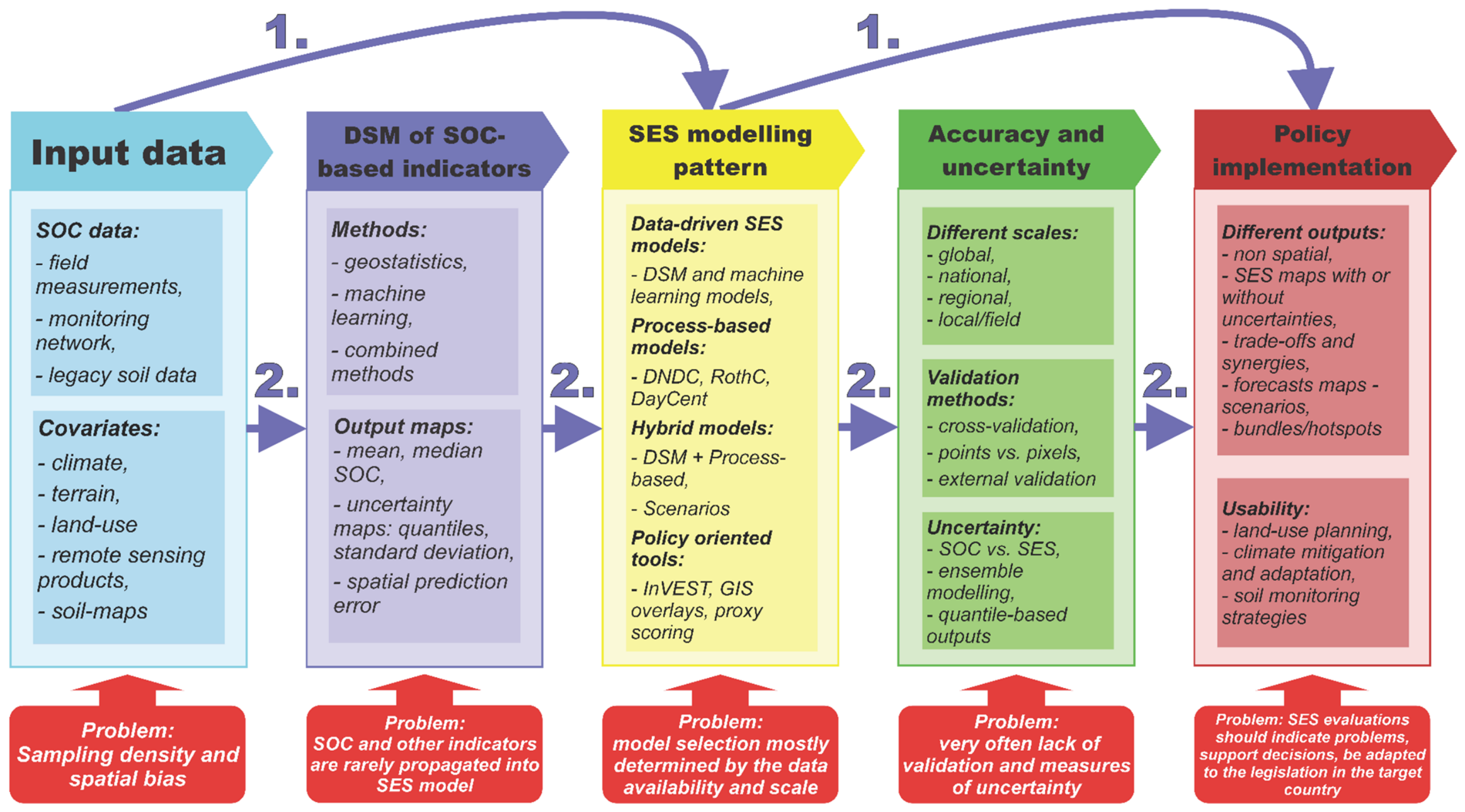
Finally, in Figure 4, we present the main outcomes of the presented systematic review. We identified two different paths of modelling, in which SESs are evaluated directly based on the input data, without visible statistical modelling, without spatial evaluation of SOC content, and without the formal validation of the results [13,21,32]. The second path shows where the complex approaches integrate all the information about the soil resources and properties [10,11,101]. These models often use digital soil mapping approaches and machine learning techniques, with the validation adapted to the map scale and uncertainty evaluation. The review shows that, despite the simplified models being common in SES assessment and policy implementation, their usability is limited due to a lack of scalability and implementation in different areas. On the other hand, all the complex approaches model the state of SES resources, are more solid for the multiscale evaluation of SESs and the analysis of land use or climate change, and provide the best possible support of land-use planning and decision making [23,93,118].

In all the SES groups, SOC data are considered as a variable, indicator, predictor, or interconnection factor as an element of the complicated soil system [40,54,114]. In many studies, the need for harmonisation of the SES modelling strategies is presented. This harmonisation must connect several modelling approaches, input the widely available data, and ensure proper validation and uncertainty propagation, especially in cases where SES maps are used for public information, policy and decision-making. Further development of the SES modelling and mapping methods will be influenced not by the development of the new indicators, but by improvements in methodological integrity, proper validation, and multiscale integration of soil data.

7. Conclusions

As the conducted research shows, the selection of methods for evaluating ecosystem services should be adapted to the scale of the study, the accessibility of a given area and its specificity. In the absence of data for a selected area, it is possible to use methods based on proxy values, such as RS or surveys, or possibly link the environmental data at our disposal with the results of previously conducted research. Process-based models use large and diverse datasets, which is why they work well for areas with high data availability and larger scales (local, regional). Empirical/statistical models are universal for various scales of studies, but they require good-quality input data. Mechanistic models can be used at various scales, but their application is closely related to the input data, and they are not methods that can be freely modified and adapted to the input data or the scale of the study. In the case of conceptual, GIS-based and proxy models, they are the most flexible and modifiable depending on the available data, the scale and the selection of indicators. For the finest scales, where the data resolution does not allow for an accurate assessment of the SES, the optimal method is direct measurements, although this is a labour-intensive and expensive method.

The results of these analyses can be translated into economic values using statistical and economic data, using deterministic models. One of the advantages of economic indicators may be to emphasise the importance of soils and their value in the context of providing specific ecosystem services. However, it should be borne in mind that the economic evaluation carries the risk of prioritising services that provide the greatest value. If one service conflicts with another (e.g., biomass production and biodiversity combined with habitat provision), by having at their disposal the results of the economic valuation, decision makers, especially developers and investors, can make decisions that contribute to environmental degradation. Therefore, the selection of indicators, methods and ways of presenting the interconnections between ecosystem services should always take into account the protection of the entire ecosystem against degradation and total devastation. As the next step, some of the methods found in this research will be applied to assess SESs on a national scale.

In each of the discussed methods of assessing 10 selected ecosystem services, SOC or SOM data can be used. Such data represent one of the basic soil parameters, and often constitute the main factor affecting the provision of ecosystem services. Their use is versatile, from the input parameter in process-based models, through the parameter used in mechanistic methods, to the proxy value of selected SES indicators. For this reason, the entity responsible for SOC monitoring should pay special attention to the quality of the databases provided, because the resulting image and assessment of ecosystem services will depend on it.

References

1. Stolte, J.; Tesfai, M.; Øygarden, L.; Kværnø, S.; Keizer, J.; Verheijen, F.; Panagos, P.; Ballabio, C.; Hessel, R. (Eds.) Soil Threats in Europe; EUR 27607 EN; Joint Research Centre: Luxembourg, 2016. [Google Scholar]
2. Pereira, P.; Bogunovic, I.; Muñoz-Rojas, M.; Brevik, E.C. Soil ecosystem services, sustainability, valuation and management. Curr. Opin. Environ. Sci. Health 2018, 5, 7–13. [Google Scholar] [CrossRef]
3. Vogel, H.-J.; Eberhardt, E.; Franko, U.; Lang, B.; Ließ, M.; Weller, U.; Wiesmeier, M.; Wollschläger, U. Quantitative Evaluation of Soil Functions: Potential and State. Front. Environ. Sci. 2019, 7, 164. [Google Scholar] [CrossRef]
4. Faber, J.H.; Cousin, I.; Meurer, K.H.E.; Hendriks, C.M.J.; Bispo, A.; Viketoft, M.; ten Damme, L.; Montagne, D.; Hanegraaf, M.C.; Gillikin, A.; et al. Stocktaking for Agricultural Soil Quality and Ecosystem Services Indicators. EJP SOIL SIREN Deliverable 2. 2022. Available online: https://edepot.wur.nl/582329 (accessed on 14 July 2023).
5. Dominati, E.; Patterson, M.; Mackay, A. A framework for classifying and quantifying the natural capital and ecosystem services of soils. Ecol. Econ. 2010, 69, 1858–1868. [Google Scholar] [CrossRef]
6. Adhikari, K.; Hartemink, A.E. Linking soils to ecosystem services—A global review. Geoderma 2016, 262, 101–111. [Google Scholar] [CrossRef]
7. European Commission. Communication from the Commission to the European Parliament, the European Council, the Council, the European Economic and Social Committee and the Committee of the Regions; COM/2019/640 Final, The European Green Deal; European Commission: Brussels, Belgium, 2021. [Google Scholar]
8. Robinson, D.A.; Hockley, N.; Dominati, E.; Lebron, I.; Scow, K.M.; Reynolds, B.; Emmett, B.A.; Keith, A.M.; de Jonge, L.W.; Schjønning, P.; et al. Natural Capital, Ecosystem Services, and Soil Change: Why Soil Science Must Embrace an Ecosystems Approach. Vadose Zone J. 2012, 11, 1–6. [Google Scholar] [CrossRef]
9. Schimel, D.S.; Participants, V.E.M.A.P.; Braswell, B.H. Continental scale variability in ecosystem processes: Models, data, and the role of disturbance. Ecol. Monogr. 1997, 67, 251–271. [Google Scholar] [CrossRef]
10. Chen, S.; Arrouays, D.; Angers, D.A.; Chenu, C.; Barré, P.; Martin, M.P.; Saby, N.P.A.; Walter, C. National estimation of soil organic carbon storage potential for arable soils: A data-driven approach coupled with carbon-landscape zones. Sci. Total Environ. 2019, 666, 355–367. [Google Scholar] [CrossRef]
11. Ma, W.; Zhan, Y.; Chen, S.; Ren, Z.; Chen, X.; Qin, F.; Lu, R.; Lv, X.; Deng, X. Organic carbon storage potential of cropland topsoils in East China: Indispensable roles of cropping systems and soil managements. Soil Tillage Res. 2021, 211, 105052. [Google Scholar] [CrossRef]
12. Singh, J.; Ale, S.; DeLaune, P.B.; Himanshu, S.K.; Barnes, E.M. Modeling the impacts of cover crops and no-tillage on soil health and cotton yield in an irrigated cropping system of the Texas Rolling Plains. Field Crops Res. 2022, 287, 108661. [Google Scholar] [CrossRef]
13. Gissi, E.; Gaglio, M.; Reho, M. Trade-off between carbon storage and biomass-based energy sources ecosystem services, the case study from the province of Rovigo (Italy). Ann. Bot. 2014, 4, 73–81. [Google Scholar] [CrossRef]
14. Calzolari, C.; Tarocco, P.; Lombardo, N.; Marchi, N.; Ungaro, F. Assessing soil ecosystem services in urban and peri-urban areas: From urban soils survey to providing support tool for urban planning. Land Use Policy 2020, 99, 105037. [Google Scholar] [CrossRef]
15. Ma, L.; Bicking, S.; Müller, F. Mapping and comparing ecosystem service indicators of global climate regulation in Schleswig-Holstein, Northern Germany. Sci. Total Environ. 2019, 648, 1582–1597. [Google Scholar] [CrossRef]
16. Zanchi, G.; Belyazid, S.; Akselsson, C.; Yu, L. Modelling the effects of management intensification on multiple forest services: A Swedish case study. Ecol. Model. 2014, 284, 48–59. [Google Scholar] [CrossRef]
17. Villoslada Peciña, M.; Ward, R.D.; Bunce, R.G.H.; Sepp, K.; Kuusemets, V.; Luuk, O. Country-scale mapping of ecosystem services provided by semi-natural grasslands. Sci. Total Environ. 2019, 661, 212–225. [Google Scholar] [CrossRef] [PubMed]
18. Yang, J.; Xie, B.; Tao, W.; Zhang, D. Ecosystem services assessment, trade-off, and bundles in the yellow river basin, China. Diversity 2021, 13, 308. [Google Scholar] [CrossRef]
19. Tricco, A.C.; Lillie, E.; Zarin, W.; O’Brien, K.K.; Colquhoun, H.; Levac, D.; Moher, D.; Peters, M.D.J.; Horsley, T.; Weeks, L.; et al. PRISMA Extension for Scoping Reviews (PRISMA-ScR): Checklist and Explanation. Ann. Intern. Med. 2018, 169, 467–473. [Google Scholar] [CrossRef] [PubMed]
20. Costanza, R.; d’Arge, R.; de Groot, R.; Farber, S.; Grasso, M.; Hannon, B.; Limburg, K.; Naeem, S.; O’Neill, R.V.; Paruelo, J.; et al. The value of the world’s ecosystem services and natural capital. Nature 1997, 387, 253–260. [Google Scholar] [CrossRef]
21. Kay, S.; Rega, C.; Moreno, G.; den Herder, M.; Palma, J.H.N.; Borek, R.; Crous-Duran, J.; Freese, D.; Giannitsopoulos, M.; Graves, A.; et al. Agroforestry creates carbon sinks whilst enhancing the environment in agricultural landscapes in Europe. Land Use Policy 2019, 83, 581–593. [Google Scholar] [CrossRef]
22. Tomscha, S.A.; Bentley, S.; Platzer, E.; Jackson, B.; de Roiste, M.; Hartley, S.; Norton, K.; Deslippe, J.R. Multiple methods confirm wetland restoration improves ecosystem services. Ecosyst. People 2021, 17, 25–40. [Google Scholar] [CrossRef]
23. Camarotto, C.; Dal Ferro, N.; Piccoli, I.; Polese, R.; Furlan, L.; Chiarini, F.; Morari, F. Conservation agriculture and cover crop practices to regulate water, carbon and nitrogen cycles in the low-lying Venetian plain. Catena 2018, 167, 236–249. [Google Scholar] [CrossRef]
24. Englund, O.; Börjesson, P.; Berndes, G.; Scarlat, N.; Dallemand, J.-F.; Grizzetti, B.; Dimitriou, I.; Mola-Yudego, B.; Fahl, F. Beneficial land use change: Strategic expansion of new biomass plantations can reduce environmental impacts from EU agriculture. Glob. Environ. Change 2020, 60, 101990. [Google Scholar] [CrossRef]
25. Abegaz, A.; Ali, A.; Tamene, L.; Abera, W.; Smith, J.U. Modeling long-term attainable soil organic carbon sequestration across the highlands of Ethiopia. Environ. Dev. Sustain. 2022, 24, 5131–5162. [Google Scholar] [CrossRef]
26. Guillaume, T.; Kotowska, M.M.; Hertel, D.; Knohl, A.; Krashevska, V.; Murtilaksono, K.; Scheu, S.; Kuzyakov, Y. Carbon costs and benefits of Indonesian rainforest conversion to plantations. Nat. Commun. 2018, 9, 2388. [Google Scholar] [CrossRef] [PubMed]
27. Pan, J.Y.; Wang, J.L.; Liu, G.J.; Gao, F. Estimation of Ecological Asset Values in Shangri-La Based on Remotely Sensed Data. Appl. Ecol. Environ. Res. 2022, 20, 2879–2895. [Google Scholar] [CrossRef]
28. Li, D.; Cao, W.; Dou, Y.; Wu, S.; Liu, J.; Li, S. Non-linear effects of natural and anthropogenic drivers on ecosystem services: Integrating thresholds into conservation planning. J. Environ. Manag. 2022, 321, 116047. [Google Scholar] [CrossRef] [PubMed]
29. Nilsson, D.; Rosenqvist, H. Profitability of crop cultivation in small arable fields when taking economic values of ecosystem services into account. Sustainability 2021, 13, 13354. [Google Scholar] [CrossRef]
30. Li, S.; Zhao, Y.; Xiao, W.; Yellishetty, M.; Yang, D. Identifying ecosystem service bundles and the spatiotemporal characteristics of trade-offs and synergies in coal mining areas with a high groundwater table. Sci. Total Environ. 2022, 807, 151036. [Google Scholar] [CrossRef]
31. Gallego-Sala, A.V.; Booth, R.K.; Charman, D.J.; Prentice, I.C.; Yu, Z. Peatlands and climate change. In Peatland Restoration and Ecosystem Services; Cambridge University Press: Cambridge, UK, 2016; pp. 129–150. [Google Scholar] [CrossRef]
32. Modernel, P.; Rossing, W.A.H.; Corbeels, M.; Dogliotti, S.; Picasso, V.; Tittonell, P. Land use change and ecosystem service provision in Pampas and Campos grasslands of southern South America. Environ. Res. Lett. 2016, 11, 113002. [Google Scholar] [CrossRef]
33. Albizua, A.; Williams, A.; Hedlund, K.; Pascual, U. Crop rotations including ley and manure can promote ecosystem services in conventional farming systems. Appl. Soil Ecol. 2015, 95, 54–61. [Google Scholar] [CrossRef]
34. Meena, R.S.; Yadav, A.; Kumar, S.; Jhariya, M.K.; Jatav, S.S. Agriculture ecosystem models for CO2 sequestration, improving soil physicochemical properties, and restoring degraded land. Ecol. Eng. 2022, 176, 106546. [Google Scholar] [CrossRef]
35. Johnston, A.S.A.; Sibly, R.M.; Hodson, M.E.; Alvarez, T.; Thorbek, P. Effects of agricultural management practices on earthworm populations and crop yield: Validation and application of a mechanistic modelling approach. J. Appl. Ecol. 2015, 52, 1334–1342. [Google Scholar] [CrossRef]
36. Zimmermann, J.; Styles, D.; Hastings, A.; Dauber, J.; Jones, M.B. Assessing the impact of within crop heterogeneity (‘patchiness’) in young Miscanthus × giganteus fields on economic feasibility and soil carbon sequestration. GCB Bioenergy 2014, 6, 566–576. [Google Scholar] [CrossRef]
37. Griffel, L.M.; Toba, A.-L.; Paudel, R.; Lin, Y.; Hartley, D.S.; Langholtz, M. A multi-criteria land suitability assessment of field allocation decisions for switchgrass. Ecol. Indic. 2022, 136, 108617. [Google Scholar] [CrossRef]
38. Gos, P.; Loucougaray, G.; Colace, M.-P.; Arnoldi, C.; Gaucherand, S.; Dumazel, D.; Girard, L.; Delorme, S.; Lavorel, S. Relative contribution of soil, management and traits to co-variations of multiple ecosystem properties in grasslands. Oecologia 2016, 180, 1001–1013. [Google Scholar] [CrossRef] [PubMed]
39. Núñez, M.; Antón, A.; Muñoz, P.; Rieradevall, J. Inclusion of soil erosion impacts in life cycle assessment on a global scale: Application to energy crops in Spain. Int. J. Life Cycle Assess. 2013, 18, 755–767. [Google Scholar] [CrossRef]
40. Piastrellini, R.; Civit, B.M.; Arena, A.P. Influence of agricultural practices on biotic production potential and climate regulation potential. A case study for life cycle assessment of soybean (Glycine max) in Argentina. Sustainability 2015, 7, 4386–4410. [Google Scholar] [CrossRef]
41. Buzhdygan, O.Y.; Tietjen, B.; Rudenko, S.S.; Nikorych, V.A.; Petermann, J.S. Direct and indirect effects of land-use intensity on plant communities across elevation in semi-natural grasslands. PLoS ONE 2020, 15, e0231122. [Google Scholar] [CrossRef] [PubMed]
42. Meyer, R.; Cullen, B.R.; Johnson, I.R.; Eckard, R.J. Process modelling to assess the sequestration and productivity benefits of soil carbon for pasture. Agric. Ecosyst. Environ. 2015, 213, 272–280. [Google Scholar] [CrossRef]
43. Sun, J.; Twine, T.E.; Hill, J.; Noe, R.; Shi, J.; Li, M. Effects of land use change for crops on water and carbon budgets in the Midwest USA. Sustainability 2017, 9, 225. [Google Scholar] [CrossRef]
44. Dai, Z.; Trettin, C.C.; Frolking, S.; Birdsey, R.A. Mangrove carbon assessment tool: Model development and sensitivity analysis. Estuar. Coast. Shelf Sci. 2018, 208, 23–35. [Google Scholar] [CrossRef]
45. Wang, H.; Dai, Z.; Trettin, C.C.; Krauss, K.W.; Noe, G.B.; Burton, A.J.; Stagg, C.L.; Ward, E.J. Modeling impacts of drought-induced salinity intrusion on carbon dynamics in tidal freshwater forested wetlands. Ecol. Appl. 2022, 32, e2700. [Google Scholar] [CrossRef]
46. Boone, R.B.; Conant, R.T.; Sircely, J.; Thornton, P.K.; Herrero, M. Climate change impacts on selected global rangeland ecosystem services. Glob. Change Biol. 2018, 24, 1382–1393. [Google Scholar] [CrossRef] [PubMed]
47. Iravani, M.; White, S.R.; Farr, D.R.; Habib, T.J.; Kariyeva, J.; Faramarzi, M. Assessing the provision of carbon-related ecosystem services across a range of temperate grassland systems in western Canada. Sci. Total Environ. 2019, 680, 151–168. [Google Scholar] [CrossRef] [PubMed]
48. Sircely, J.; Conant, R.T.; Boone, R.B. Simulating Rangeland Ecosystems with G-Range: Model Description and Evaluation at Global and Site Scales. Rangel. Ecol. Manag. 2019, 72, 846–857. [Google Scholar] [CrossRef]
49. Ma, K.; Liu, J.; Balkovič, J.; Skalský, R.; Azevedo, L.B.; Kraxner, F. Changes in soil organic carbon stocks of wetlands on China’s Zoige plateau from 1980 to 2010. Ecol. Model. 2016, 327, 18–28. [Google Scholar] [CrossRef]
50. Yu, D.; Qiao, J.; Shi, P. Spatiotemporal patterns, relationships, and drivers of China’s agricultural ecosystem services from 1980 to 2010: A multiscale analysis. Landsc. Ecol. 2018, 33, 575–595. [Google Scholar] [CrossRef]
51. Quemada, M.; Lassaletta, L.; Leip, A.; Jones, A.; Lugato, E. Integrated management for sustainable cropping systems: Looking beyond the greenhouse balance at the field scale. Glob. Change Biol. 2020, 26, 2584–2598. [Google Scholar] [CrossRef]
52. Ghaley, B.B.; Porter, J.R. Ecosystem function and service quantification and valuation in a conventional winter wheat production system with DAISY model in Denmark. Ecosyst. Serv. 2014, 10, 79–83. [Google Scholar] [CrossRef]
53. Cong, R.-G.; Termansen, M.; Brady, M.V. Managing soil natural capital: A prudent strategy for adapting to future risks. Ann. Oper. Res. 2017, 255, 439–463. [Google Scholar] [CrossRef]
54. Zhao, F.; Wu, Y.; Qiu, L.; Sivakumar, B.; Zhang, F.; Sun, Y.; Sun, L.; Li, Q.; Voinov, A. Spatiotemporal features of the hydro-biogeochemical cycles in a typical loess gully watershed. Ecol. Indic. 2018, 91, 542–554. [Google Scholar] [CrossRef]
55. Valipour, M.; Johnson, C.E.; Battles, J.J.; Campbell, J.L.; Fahey, T.J.; Fakhraei, H.; Driscoll, C.T. Forest harvesting under climate change. Sci. Total Environ. 2021, 767, 144881. [Google Scholar] [CrossRef]
56. Wicaksono, P.; Hartono, P.D.; Nehren, U. Mangrove biomass carbon stock mapping of the Karimunjawa Islands using multispectral remote sensing. Int. J. Remote Sens. 2016, 37, 26–52. [Google Scholar] [CrossRef]
57. Tóth, G.; Gardi, C.; Bódis, K.; Ivits, É.; Aksoy, E.; Jones, A.; Jeffrey, S.; Petursdottir, T.; Montanarella, L. Continental-scale assessment of provisioning soil functions in Europe. Ecol. Process. 2013, 2, 32. [Google Scholar] [CrossRef]
58. Sever, M.Z.O.; Alberti, G.; Delle Vedove, G.; Marjanović, H. Temporal evolution of carbon stocks, fluxes and carbon balance in pedunculate oak chronosequence under close-to-nature forest management. Forests 2019, 10, 814. [Google Scholar] [CrossRef]
59. Kounnamas, C.; Andreou, M. Mapping and assessment of ecosystem services at Troodos National Forest Park in Cyprus. One Ecosyst. 2022, 7, e77584. [Google Scholar] [CrossRef]
60. Habib-ur-Rahman, M.; Raza, A.; Ahrends, H.E.; Hüging, H.; Gaiser, T. Impact of in-field soil heterogeneity on biomass and yield of winter triticale in an intensively cropped hummocky landscape under temperate climate conditions. Precis. Agric. 2022, 23, 912–938. [Google Scholar] [CrossRef]
61. Kirchner, M.; Schmidt, J.; Kindermann, G.; Kulmer, V.; Mitter, H.; Prettenthaler, F.; Rüdisser, J.; Schauppenlehner, T.; Schönhart, M.; Strauss, F.; et al. Ecosystem services and economic development in Austrian agricultural landscapes—The impact of policy and climate change scenarios on trade-offs and synergies. Ecol. Econ. 2015, 109, 161–174. [Google Scholar] [CrossRef]
62. Cong, R.-G.; Hedlund, K.; Andersson, H.; Brady, M. Managing soil natural capital: An effective strategy for mitigating future agricultural risks? Agric. Syst. 2014, 129, 30–39. [Google Scholar] [CrossRef]
63. Thaler, E.A.; Larsen, I.J.; Yu, Q. The extent of soil loss across the US Corn Belt. Proc. Natl. Acad. Sci. USA 2021, 118, e1922375118. [Google Scholar] [CrossRef]
64. Zhang, X.; Izaurralde, R.C.; Manowitz, D.H.; Sahajpal, R.; West, T.O.; Thomson, A.M.; Xu, M.; Zhao, K.; LeDuc, S.D.; Williams, J.R. Regional scale cropland carbon budgets: Evaluating a geospatial agricultural modeling system using inventory data. Environ. Model. Softw. 2015, 63, 199–216. [Google Scholar] [CrossRef]
65. Richter, S.; Haase, D.; Thestorf, K.; Makki, M. Carbon Pools of Berlin, Germany: Organic Carbon in Soils and Aboveground in Trees. Urban For. Urban Green. 2020, 54, 126777. [Google Scholar] [CrossRef]
66. Jungkunst, H.F.; Göpel, J.; Horvath, T.; Ott, S.; Brunn, M. Global soil organic carbon–climate interactions: Why scales matter. Wiley Interdiscip. Rev. Clim. Change 2022, 13, e780. [Google Scholar] [CrossRef]
67. Creamer, R.E.; Hannula, S.E.; Van Leeuwen, J.P.; Stone, D.; Rutgers, M.; Schmelz, R.M.; De Ruiter, P.C.; Hendriksen, N.B.; Bolger, T.; Bouffaud, M.L.; et al. Ecological network analysis reveals the inter-connection between soil biodiversity and ecosystem function as affected by land use across Europe. Appl. Soil Ecol. 2016, 97, 112–124. [Google Scholar] [CrossRef]
68. Dong, X.; Yang, W.; Ulgiati, S.; Yan, M.; Zhang, X. The impact of human activities on natural capital and ecosystem services of natural pastures in North Xinjiang, China. Ecol. Model. 2012, 225, 28–39. [Google Scholar] [CrossRef]
69. Van Wijnen, H.J.; Rutgers, M.; Schouten, A.J.; Mulder, C.; de Zwart, D.; Breure, A.M. How to calculate the spatial distribution of ecosystem services—Natural attenuation as example from The Netherlands. Sci. Total Environ. 2012, 415, 49–55. [Google Scholar] [CrossRef]
70. Makovníková, J.; Kanianska, R.; Kizeková, M. The ecosystem services supplied by soil in relation to land use. Hung. Geogr. Bull. 2017, 66, 37–42. [Google Scholar] [CrossRef]
71. Delavaran, H.; Kazemi, H.; Kamkar, B.; Gherekhloo, J. Development of a new model for health assessment in agroecosystems. Environ. Monit. Assess. 2022, 194, 78. [Google Scholar] [CrossRef]
72. Freschet, G.T.; Masse, D.; Hien, E.; Sall, S.; Chotte, J.-L. Long-term changes in organic matter and microbial properties resulting from manuring practices in an arid cultivated soil in Burkina Faso. Agric. Ecosyst. Environ. 2008, 123, 175–184. [Google Scholar] [CrossRef]
73. Sircely, J.; Naeem, S. Biodiversity and Ecosystem Multi-Functionality: Observed Relationships in Smallholder Fallows in Western Kenya. PLoS ONE 2012, 7, e50152. [Google Scholar] [CrossRef]
74. Baskan, O.; Dengiz, O.; Demirag, İ.T. The land productivity dynamics trend as a tool for land degradation assessment in a dryland ecosystem. Environ. Monit. Assess. 2017, 189, 212. [Google Scholar] [CrossRef]
75. Mendez-Estrella, R.; Romo-Leon, J.R.; Castellanos, A.E. Mapping changes in carbon storage and productivity services provided by riparian ecosystems of semi-arid environments in northwestern Mexico. ISPRS Int. J. Geo-Inf. 2017, 6, 298. [Google Scholar] [CrossRef]
76. Bartholomée, O.; Grigulis, K.; Colace, M.-P.; Arnoldi, C.; Lavorel, S. Methodological uncertainties in estimating carbon storage in temperate forests and grasslands. Ecol. Indic. 2018, 95, 331–342. [Google Scholar] [CrossRef]
77. Gebeyehu, G.; Soromessa, T.; Bekele, T.; Teketay, D. Carbon stocks and factors affecting their storage in dry Afromontane forests of Awi Zone, northwestern Ethiopia. J. Ecol. Environ. 2019, 43, 7. [Google Scholar] [CrossRef]
78. Hou, Z.; Lv, G.; Jiang, L. Functional diversity can predict ecosystem functions better than dominant species: The case of desert plants in the Ebinur lake basin. Sustainability 2021, 13, 2858. [Google Scholar] [CrossRef]
79. Ntukey, L.T.; Munishi, L.K.; Treydte, A.C. Land Use Land/Cover Change Reduces Woody Plant Diversity and Carbon Stocks in a Lowland Coastal Forest Ecosystem, Tanzania. Sustainability 2022, 14, 8551. [Google Scholar] [CrossRef]
80. Morais, T.G.; Teixeira, R.F.; Rodrigues, N.R.; Domingos, T. Characterizing livestock production in Portuguese sown rainfed grasslands: Applying the inverse approach to a process-based model. Sustainability 2018, 10, 4437. [Google Scholar] [CrossRef]
81. Jebari, A.; Álvaro-Fuentes, J.; Pardo, G.; Batalla, I.; Martín, J.A.R.; Del Prado, A. Effect of dairy cattle production systems on sustaining soil organic carbon storage in grasslands of northern Spain. Reg. Environ. Change 2022, 22, 67. [Google Scholar] [CrossRef]
82. Baldassini, P.; Paruelo, J.M. Deforestation and current management practices reduce soil organic carbon in the semi-arid Chaco, Argentina. Agric. Syst. 2020, 178, 102749. [Google Scholar] [CrossRef]
83. Sil, Â.; Fonseca, F.; Gonçalves, J.; Honrado, J.; Marta-Pedroso, C.; Alonso, J.; Ramos, M.; Azevedo, J.C. Analysing carbon sequestration and storage dynamics in a changing mountain landscape in Portugal: Insights for management and planning. Int. J. Biodivers. Sci. Ecosyst. Serv. Manag. 2017, 13, 82–104. [Google Scholar] [CrossRef]
84. Raj Kumar, K.V.G.; Barik, D.K. Assessment of carbon storage and erosion using invest model in Visakhapatnam district, Andhra Pradesh. J. Rural Dev. 2018, 37, 207–220. [Google Scholar] [CrossRef]
85. Zarandian, A.; Badamfirouz, J.; Musazadeh, R.; Rahmati, A.; Azimi, S.B. Scenario modeling for spatial-temporal change detection of carbon storage and sequestration in a forested landscape in Northern Iran. Environ. Monit. Assess. 2018, 190, 474. [Google Scholar] [CrossRef]
86. Xiang, H.; Wang, Z.; Mao, D.; Zhang, J.; Xi, Y.; Du, B.; Zhang, B. What did China’s National Wetland Conservation Program Achieve? Observations of changes in land cover and ecosystem services in the Sanjiang Plain. J. Environ. Manag. 2020, 267, 110623. [Google Scholar] [CrossRef]
87. Zhang, X.; Wang, J.; Yue, C.; Ma, S.; Wang, L.-J. Exploring the spatiotemporal changes in carbon storage under different development scenarios in Jiangsu Province, China. PeerJ 2022, 10, e13411. [Google Scholar] [CrossRef]
88. Lu, N.; Akujärvi, A.; Wu, X.; Liski, J.; Wen, Z.; Holmberg, M.; Feng, X.; Zeng, Y.; Fu, B. Changes in soil carbon stock predicted by a process-based soil carbon model (Yasso07) in the Yanhe watershed of the Loess Plateau. Landsc. Ecol. 2015, 30, 399–413. [Google Scholar] [CrossRef]
89. Nguyen, T.H.; Nong, D.; Paustian, K. Surrogate-based multi-objective optimization of management options for agricultural landscapes using artificial neural networks. Ecol. Model. 2019, 400, 1–13. [Google Scholar] [CrossRef]
90. Longo, M.; Dal Ferro, N.; Lazzaro, B.; Morari, F. Trade-offs among ecosystem services advance the case for improved spatial targeting of agri-environmental measures. J. Environ. Manag. 2021, 285, 112131. [Google Scholar] [CrossRef]
91. Masikati, P.; Sisito, G.; Chipatela, F.; Tembo, H.; Winowiecki, L.A. Agriculture extensification and associated socio-ecological trade-offs in smallholder farming systems of Zambia. Int. J. Agric. Sustain. 2021, 19, 497–508. [Google Scholar] [CrossRef]
92. Cardinael, R.; Guenet, B.; Chevallier, T.; Dupraz, C.; Cozzi, T.; Chenu, C. High organic inputs explain shallow and deep SOC storage in a long-term agroforestry system—Combining experimental and modeling approaches. Biogeosciences 2018, 15, 297–317. [Google Scholar] [CrossRef]
93. Xu, X.; Liu, J.; Tan, Y.; Yang, G. Quantifying and optimizing agroecosystem services in China’s Taihu Lake Basin. J. Environ. Manag. 2021, 277, 111440. [Google Scholar] [CrossRef]
94. Zhang, Y.; Paustian, K. Sensitivity of predicted agro-ecosystem variables to errors in weather input data. Trans. ASABE 2019, 62, 627–640. [Google Scholar] [CrossRef]
95. Pillar, V.D.; Tornquist, C.G.; Bayer, C. The southern Brazilian grassland biome: Soil carbon stocks, fluxes of greenhouse gases and some options for mitigation [Campos do sul do Brasil: Estoques de carbono no solo, fluxos de gases de efeito estufa e algumas opções para mitigação]. Braz. J. Biol. 2012, 72, 673–681. [Google Scholar] [CrossRef]
96. Grossman, J.J. Ecosystem service trade-offs and land use among smallholder farmers in Eastern Paraguay. Ecol. Soc. 2015, 20, 19. [Google Scholar] [CrossRef]
97. Nguyen, T.H.; Cook, M.; Field, J.L.; Khuc, Q.V.; Paustian, K. High-resolution trade-off analysis and optimization of ecosystem services and disservices in agricultural landscapes. Environ. Model. Softw. 2018, 107, 105–118. [Google Scholar] [CrossRef]
98. Portalanza, D.; Barral, M.P.; Villa-Cox, G.; Ferreira-Estafanous, S.; Herrera, P.; Durigon, A.; Ferraz, S. Mapping ecosystem services in a rural landscape dominated by cacao crop: A case study for Los Rios province, Ecuador. Ecol. Indic. 2019, 107, 105593. [Google Scholar] [CrossRef]
99. Burke, S.; Poncé-Hernandez, R. Connecting the Water and Carbon Cycles for the Generation of Food Security and Ecosystem Services. Future Food J. 2019, 2, 8–20. [Google Scholar]
100. Byrd, K.B.; Flint, L.E.; Alvarez, P.; Casey, C.F.; Sleeter, B.M.; Soulard, C.E.; Flint, A.L.; Sohl, T.L. Integrated climate and land use change scenarios for California rangeland ecosystem services: Wildlife habitat, soil carbon, and water supply. Landsc. Ecol. 2015, 30, 729–750. [Google Scholar] [CrossRef]
101. Hübner, R.; Kühnel, A.; Lu, J.; Dettmann, H.; Wang, W.; Wiesmeier, M. Soil carbon sequestration by agroforestry systems in China: A meta-analysis. Agric. Ecosyst. Environ. 2021, 315, 107437. [Google Scholar] [CrossRef]
102. Li, J.; Li, M.; Dong, L.; Wang, K.; Liu, Y.; Hai, X.; Pan, Y.; Lv, W.; Wang, X.; Shangguan, Z.; et al. Plant productivity and microbial composition drive soil carbon and nitrogen sequestrations following cropland abandonment. Sci. Total Environ. 2020, 744, 140802. [Google Scholar] [CrossRef]
103. Mi, J.; Liu, W.; Yang, W.; Yan, J.; Li, J.; Sang, T. Carbon sequestration by Miscanthus energy crops plantations in a broad range semi-arid marginal land in China. Sci. Total Environ. 2014, 496, 373–380. [Google Scholar] [CrossRef]
104. Chu, X.; Zhan, J.; Li, Z.; Zhang, F.; Qi, W. Assessment on forest carbon sequestration in the Three-North Shelterbelt Program region, China. J. Clean. Prod. 2019, 215, 382–389. [Google Scholar] [CrossRef]
105. Xu, G.; Xiong, K.; Shu, T.; Shi, Y.; Chen, L.; Zheng, L.; Fan, H.; Zhao, Z.; Yang, Z. Bundling evaluating changes in ecosystem service under karst rocky desertification restoration: Projects a case study of Huajiang-Guanling, Guizhou province, Southwest China. Environ. Earth Sci. 2022, 81, 302. [Google Scholar] [CrossRef]
106. Qi, J.; Du, X.; Zhang, X.; Lee, S.; Wu, Y.; Deng, J.; Moglen, G.E.; Sadeghi, A.M.; McCarty, G.W. Modeling riverine dissolved and particulate organic carbon fluxes from two small watersheds in the northeastern United States. Environ. Model. Softw. 2020, 124, 104601. [Google Scholar] [CrossRef]
107. Yu, Y.; Li, J.; Zhou, Z.; Zeng, L.; Zhang, C. Estimation of the value of ecosystem carbon sequestration services under different scenarios in the central China (The Qinling-Daba mountain area). Sustainability 2020, 12, 337. [Google Scholar] [CrossRef]
108. Zhu, Z.; Bouchard, M.; Butman, D.; Hawbaker, T.; Li, Z.; Liu, J.; Liu, S.; McDonald, C.; Reker, R.; Sayler, K.; et al. Baseline and Projected Future Carbon Storage and Greenhouse-Gas Fluxes in the Great Plains Region of the United States; Professional Paper No. 1787; U.S. Geological Survey: Reston, VA, USA, 2011; pp. 1–31.
109. Biffi, S.; Chapman, P.J.; Grayson, R.P.; Ziv, G. Soil carbon sequestration potential of planting hedgerows in agricultural landscapes. J. Environ. Manag. 2022, 307, 114484. [Google Scholar] [CrossRef]
110. Ranathunga, K.N.; Finke, P.A.; Yin, Q.; Verdoodt, A.; Yu, Y. Soil modeling for soil loss tolerance estimations: Exploring natural baselines and long-term variations. Glob. Planet. Change 2021, 204, 103548. [Google Scholar] [CrossRef]
111. Lange, M.; Eisenhauer, N.; Sierra, C.A.; Bessler, H.; Engels, C.; Griffiths, R.I.; Mellado-Vázquez, P.G.; Malik, A.A.; Roy, J.; Scheu, S.; et al. Plant diversity increases soil microbial activity and soil carbon storage. Nat. Commun. 2015, 6, 6707. [Google Scholar] [CrossRef]
112. Vuichard, N.; Ciais, P.; Wolf, A. Soil carbon sequestration or biofuel production: New land-use opportunities for mitigating climate over abandoned soviet farmlands. Environ. Sci. Technol. 2009, 43, 8678–8683. [Google Scholar] [CrossRef]
113. Weslien, J.; Finér, L.; Jónsson, J.A.; Koivusalo, H.; Laurén, A.; Ranius, T.; Sigurdsson, B.D. Effects of increased forest productivity and warmer climates on carbon sequestration, run-off water quality and accumulation of dead wood in a boreal landscape: A modelling study. Scand. J. For. Res. 2009, 24, 333–347. [Google Scholar] [CrossRef]
114. Yu, Y.; Sun, X.; Wang, J.; Zhang, J. Using InVEST to evaluate water yield services in Shangri-La, Northwestern Yunnan, China. PeerJ 2022, 10, e12804. [Google Scholar] [CrossRef]
115. Meshesha, T.W.; Wang, J.; Melaku, N.D. Modelling spatiotemporal patterns of water quality and its impacts on aquatic ecosystem in the cold climate region of Alberta, Canada. J. Hydrol. 2020, 587, 124952. [Google Scholar] [CrossRef]
116. Voss, M.; Dippner, J.W.; Humborg, C.; Hürdler, J.; Korth, F.; Neumann, T.; Schernewski, G.; Venohr, M. History and scenarios of future development of Baltic Sea eutrophication. Estuar. Coast. Shelf Sci. 2011, 92, 307–322. [Google Scholar] [CrossRef]
117. Palmer, J.; Thorburn, P.J.; Biggs, J.S.; Dominati, E.J.; Probert, M.E.; Meier, E.A.; Huth, N.I.; Dodd, M.; Snow, V.; Larsen, J.R.; et al. Nitrogen cycling from increased soil organic carbon contributes both positively and negatively to ecosystem services in wheat agro-ecosystems. Front. Plant Sci. 2017, 8, 731. [Google Scholar] [CrossRef] [PubMed]
118. Shili-Touzi, I.; De Tourdonnet, S.; Launay, M.; Dore, T. Does intercropping winter wheat (Triticum aestivum) with red fescue (Festuca rubra) as a cover crop improve agronomic and environmental performance? A modeling approach. Field Crops Res. 2010, 116, 218–229. [Google Scholar] [CrossRef]
119. Williams, A.; Davis, A.S.; Jilling, A.; Grandy, A.S.; Koide, R.T.; Mortensen, D.A.; Smith, R.G.; Snapp, S.S.; Spokas, K.A.; Yannarell, A.C.; et al. Reconciling opposing soil processes in row-crop agroecosystems via soil functional zone management. Agric. Ecosyst. Environ. 2017, 236, 99–107. [Google Scholar] [CrossRef]
120. Pommier, T.; Cantarel, A.A.M.; Grigulis, K.; Lavorel, S.; Legay, N.; Baxendale, C.; Bardgett, R.D.; Bahn, M.; Poly, F.; Clément, J.-C. The added value of including key microbial traits to determine nitrogen-related ecosystem services in managed grasslands. J. Appl. Ecol. 2018, 55, 49–58. [Google Scholar] [CrossRef]
121. Giguère-Tremblay, R.; Laperriere, G.; de Grandpré, A.; Morneault, A.; Bisson, D.; Chagnon, P.-L.; Germain, H.; Maire, V. Boreal forest multifunctionality is promoted by low soil organic matter content and high regional bacterial biodiversity in Northeastern Canada. Forests 2020, 11, 149. [Google Scholar] [CrossRef]
122. Gao, Z.; Niu, F.; Wang, Y.; Luo, J.; Lin, Z. Impact of a thermokarst lake on the soil hydrological properties in permafrost regions of the Qinghai-Tibet Plateau, China. Sci. Total Environ. 2017, 574, 751–759. [Google Scholar] [CrossRef]
123. Xu, S.; Liu, Y.; Wang, X.; Zhang, G. Scale effect on spatial patterns of ecosystem services and associations among them in semi-arid area: A case study in Ningxia Hui Autonomous Region, China. Sci. Total Environ. 2017, 598, 297–306. [Google Scholar] [CrossRef]
124. De Valença, A.W.; Vanek, S.J.; Meza, K.; Ccanto, R.; Olivera, E.; Scurrah, M.; A Lantinga, E.; Fonte, S.J. Land use as a driver of soil fertility and biodiversity across an agricultural landscape in the Central Peruvian Andes. Ecol. Appl. 2017, 27, 1138–1154. [Google Scholar] [CrossRef]
125. Andrés, P.; Moore, J.C.; Simpson, R.T.; Selby, G.; Cotrufo, F.; Denef, K.; Haddix, M.L.; Shaw, E.A.; de Tomasel, C.M.; Molowny-Horas, R.; et al. Soil food web stability in response to grazing in a semi-arid prairie: The importance of soil textural heterogeneity. Soil Biol. Biochem. 2016, 97, 131–143. [Google Scholar] [CrossRef]
126. Guan, Z.; Lin, D.; Chen, D.; Guo, Y.; Lu, Y.; Han, Q.; Li, N.; Su, Y.; Li, J.; Wang, J.; et al. Soil microbial communities response to different fertilization regimes in young Catalpa bungei plantation. Front. Microbiol. 2022, 13, 948875. [Google Scholar] [CrossRef]
127. Goulnik, J.; Plantureux, S.; Théry, M.; Baude, M.; Delattre, M.; van Reeth, C.; Villerd, J.; Michelot-Antalik, A. Floral trait functional diversity is related to soil characteristics and positively influences pollination function in semi-natural grasslands. Agric. Ecosyst. Environ. 2020, 301, 107033. [Google Scholar] [CrossRef]
128. Wan, X.; Chen, X.; Huang, Z.; Chen, H.Y.H. Global soil microbial biomass decreases with aridity and land-use intensification. Glob. Ecol. Biogeogr. 2021, 30, 1056–1069. [Google Scholar] [CrossRef]
129. Yang, K.H.; Cho, J.-S.; Kim, J.-E.; Hong, S.-K.; Choi, J.-W.; Park, S.B.; Lee, J.-S.; Ju, H.G.; Myeong, H.-H.; Yang, H.-S.; et al. Distribution Strategies of Vascular Plants at the Reclaimed Lands at the Saemangum Sea Dike. J. Mar. Isl. Cult. 2021, 10, 45–57. [Google Scholar] [CrossRef]
130. Rutgers, M.; van Leeuwen, J.P.; Vrebos, D.; van Wijnen, H.J.; Schouten, T.; de Goede, R.G.M. Mapping soil biodiversity in Europe and the Netherlands. Soil Syst. 2019, 3, 39. [Google Scholar] [CrossRef]
131. Tian, J.; He, N.; Hale, L.; Niu, S.; Yu, G.; Liu, Y.; Blagodatskaya, E.; Kuzyakov, Y.; Gao, Q.; Zhou, J. Soil organic matter availability and climate drive latitudinal patterns in bacterial diversity from tropical to cold temperate forests. Funct. Ecol. 2018, 32, 61–70. [Google Scholar] [CrossRef]
132. Aksoy, E.; Louwagie, G.; Gardi, C.; Gregor, M.; Schröder, C.; Löhnertz, M. Assessing soil biodiversity potentials in Europe. Sci. Total Environ. 2017, 589, 236–249. [Google Scholar] [CrossRef] [PubMed]
133. van Leeuwen, J.P.; Creamer, R.E.; Cluzeau, D.; Debeljak, M.; Gatti, F.; Henriksen, C.B.; Kuzmanovski, V.; Menta, C.; Pérès, G.; Picaud, C.; et al. Modeling of Soil Functions for Assessing Soil Quality: Soil Biodiversity and Habitat Provisioning. Front. Environ. Sci. 2019, 7, 113. [Google Scholar] [CrossRef]
134. Lohrer, A.M.; Stephenson, F.; Douglas, E.J.; Townsend, M. Mapping the estuarine ecosystem service of pollutant removal using empirically validated boosted regression tree models. Ecol. Appl. 2020, 30, e02105. [Google Scholar] [CrossRef]
135. Li, M.; Li, X.; Liu, S.; Li, X.; Lyu, X.; Dang, D.; Dou, H. Ecosystem services under different grazing intensities in typical grasslands in Inner Mongolia and their relationships. Glob. Ecol. Conserv. 2021, 26, e01526. [Google Scholar] [CrossRef]
136. Xie, T.; Wang, M.; Su, C.; Chen, W. Evaluation of the natural attenuation capacity of urban residential soils with ecosystem-service performance index (EPX) and entropy-weight methods. Environ. Pollut. 2018, 238, 222–229. [Google Scholar] [CrossRef]
137. Zhang, X.; Zhu, W.; Yan, N.; Wei, P.; Zhao, Y.; Zhao, H.; Zhu, L. Research on Service Value and Adaptability Zoning of Grassland Ecosystem in Ethiopia. Remote Sens. 2022, 14, 2722. [Google Scholar] [CrossRef]
138. Laporta, L.; Domingos, T.; Marta-Pedroso, C. Mapping and assessment of ecosystems services under the proposed maes european common framework: Methodological challenges and opportunities. Land 2021, 10, 1040. [Google Scholar] [CrossRef]
139. Froger, C.; Tondini, E.; Arrouays, D.; Oorts, K.; Poeplau, C.; Wetterlind, J.; Putku, E.; Saby, N.P.A.; Fantappiè, M.; Styc, Q.; et al. Comparing LUCAS Soil and national systems: Towards a harmonized European Soil monitoring network. Geoderma 2024, 449, 117027. [Google Scholar] [CrossRef]
140. Lohbeck, M.; Winowiecki, L.; Aynekulu, E.; Okia, C.; Vågen, T.-G. Trait-based approaches for guiding the restoration of degraded agricultural landscapes in East Africa. J. Appl. Ecol. 2018, 55, 59–68. [Google Scholar] [CrossRef]
141. Schneider, F.D.; Ferraz, A.; Hancock, S.; Duncanson, L.I.; Dubayah, R.O.; Pavlick, R.P.; Schimel, D.S. Towards mapping the diversity of canopy structure from space with GEDI. Environ. Res. Lett. 2020, 15, 115006. [Google Scholar] [CrossRef]
142. Vandandorj, S.; Eldridge, D.J.; Travers, S.K.; Delgado-Baquerizo, M. Contrasting Effects of Aridity and Grazing Intensity on Multiple Ecosystem Functions and Services in Australian Woodlands. Land Degrad. Dev. 2017, 28, 2098–2108. [Google Scholar] [CrossRef]
143. Glendell, M.; Jones, R.; Dungait, J.A.J.; Meusburger, K.; Schwendel, A.C.; Barclay, R.; Barker, S.; Haley, S.; Quine, T.A.; Meersmans, J. Tracing of particulate organic C sources across the terrestrial-aquatic continuum, a case study at the catchment scale (Carminowe Creek, southwest England). Sci. Total Environ. 2018, 616–617, 1077–1088. [Google Scholar] [CrossRef]
144. Jankowski, M.; Bednarek, R. Rusty soil—Gleba rdzawa—Soil of the Year 2021 in Poland. Concepts of genesis, classification and regularities of geographical distribution. Soil Sci. Annu. 2021, 72, 145585. [Google Scholar] [CrossRef]
145. Sewerniak, P. Plant species richness or soil fertility: Which affects more the productivity of Scots pine in Central Europe? Ann. For. Res. 2020, 63, 57–73. [Google Scholar] [CrossRef]
Figure 1. Review process according to PRISMA rules.
Agronomy 16 01072 g001
Figure 2. Spatial distribution of study areas of the selected articles.
Agronomy 16 01072 g002
Figure 3. The use of modelling validation parameters. The word cloud shows the use of modelling validation parameters. The higher the text frequency, the larger the font.
Agronomy 16 01072 g003
Figure 4. Framework for SOC-based SES assessment and policy implementation across scales. (1. Simplified modelling pathways, where SES assessments are created directly from input data without DSM-based modelling without validation, 2. A comprehensive modelling workflow that integrates DSM-derived SOC data, and scale-aware validation and uncertainty propagation into SES modelling).
Agronomy 16 01072 g004