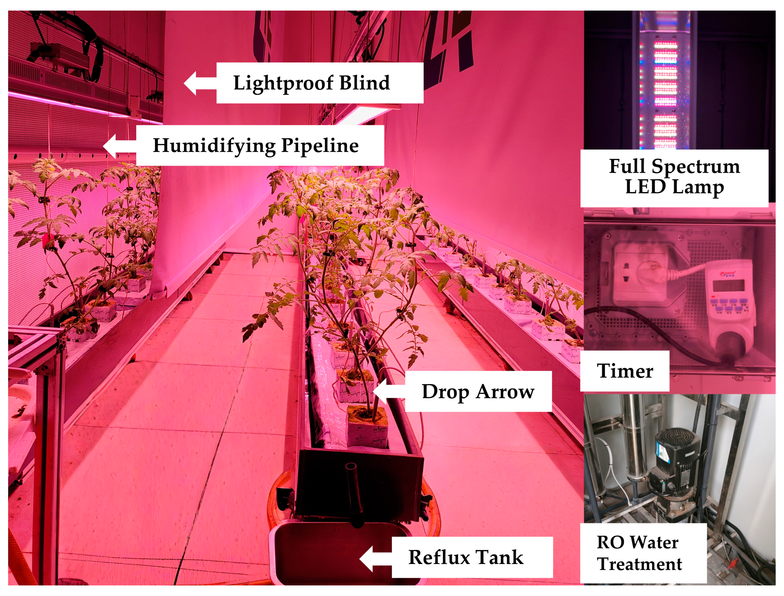
2.2. Experimental Design
This study employed a completely randomized design with nine treatments, each replicated three times, resulting in twenty-seven experimental units. The experimental treatments are listed in
Table 1. The experiment included two factors: temperature and light. Light is represented by photosynthetically active radiation (PAR), which is the visible light spectrum that can be absorbed and utilized by plants for photosynthesis, serving as a core indicator for assessing the energy supply for plant photosynthesis. PAR is quantified as photosynthetic photon flux density (PPFD) [
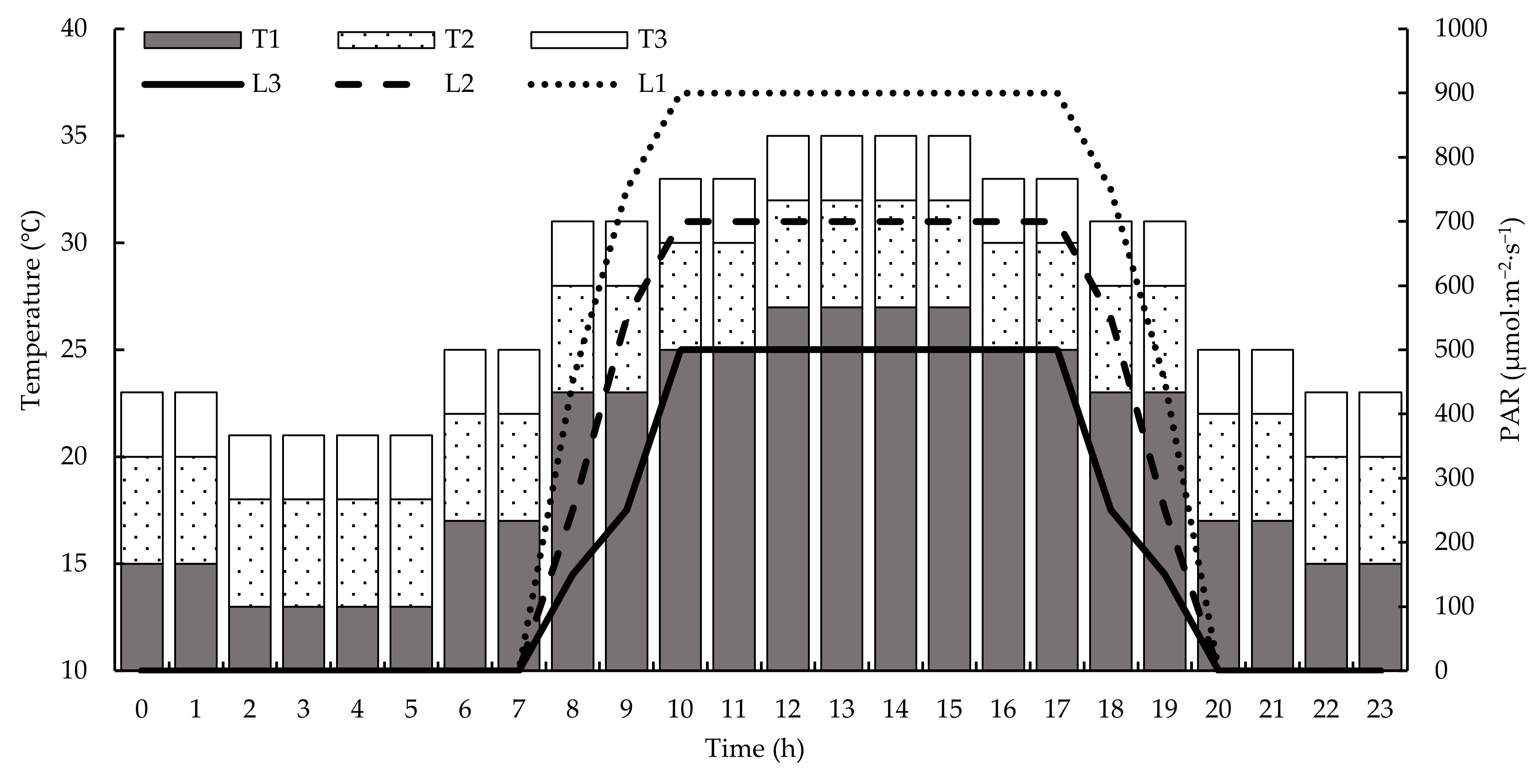
30]. The chambers simulated the diurnal variation of a 24 h greenhouse environment. Starting from 06:00, the temperature was programmed to rise gradually from its daily minimum, peak at 12:00, hold constant for 4 h, and then gradually decrease. The temperature levels were as follows:
The control temperature (T1: 25/15 °C) had an average day/night temperature of 25 ± 2/15 ± 2 °C, with a daily maximum of 27 °C and a daily minimum of 13 °C. Moderately high temperature (T2: 30/20 °C) had an average day/night temperature of 30 ± 2/20 ± 2 °C, with a daily maximum of 32 °C and a daily minimum of 18 °C. High temperature (T3: 30/20 °C) had an average day/night temperature of 35 ± 2/25 ± 2 °C, with a daily maximum of 37 °C and a daily minimum of 23 °C. However, poor fruit set was observed in T3 during preliminary trials; therefore, the temperature of T3 was reduced by 2 °C after 40 days of transplanting, resulting in adjusted conditions: a day/night temperature of 33 ± 2/23 ± 2 °C, a daily maximum temperature of 35 °C, and a daily minimum temperature of 21 °C. To comprehensively characterize the cumulative heat accumulation throughout the entire experimental process, this study summed the daily average temperatures across all stages and divided them by the total number of growing days. This yielded an average temperature of 29 °C for the entire growing period, which was used as the basis for analysis. The PAR was programmed to simulate a 24 h greenhouse photoperiod. The light was set from 08:00, with PAR increasing from its daily minimum to a maximum at 10:00. This peak level was sustained until 17:00, after which the PAR decreased hourly until reaching complete darkness at 20:00, which was maintained throughout the night. Three PAR gradients were established under a 12 h photoperiod: For normal PAR (L1), the average light intensity was 800 μmol·m
−2·s
−1, with a daily maximum of 900 μmol·m
−2·s
−1 and a daily minimum of 450 μmol·m
−2·s
−1. For medium-low PAR (L2), the average light intensity was 600 μmol·m
−2·s
−1, with a daily maximum of 700 μmol·m
−2·s
−1 and a daily minimum of 250 μmol·m
−2·s
−1. For low PAR (L3), the average light intensity was 400 μmol·m
−2·s
−1, with a daily maximum of 500 μmol·m
−2·s
−1 and a daily minimum of 150 μmol·m
−2·s
−1. Environmental changes are shown in
Figure 2.
2.3. Experimental Materials and Cultivation Management
The experiment used the tomato hybrid ‘Zhongza 1721’, an indeterminate cultivar developed by the Institute of Vegetables and Flowers, the Chinese Academy of Agricultural Sciences. This medium-early maturing cultivar exhibits vigorous growth, moderately sized leaves, and strong environmental adaptability. The mature fruits are pink, uniform in size, and round to oblate in shape, with high firmness. The trial utilized rockwool cultivation, with transplanting conducted after the flowering of the first inflorescence. The planting density was 2.5 plants·m
−2. A spacing of 0.5 m between plants within rows was maintained, with 1.6 m between rows. Each climate chamber covered an area of 25 m
2. After the seedlings had adapted for 10 days, the environmental parameters were set. Irrigation was applied using the Yamazaki nutrient solution formula via drip irrigation [
31].
The primary nutrients in this formulation are shown in
Table 2.
All treatments employed identical drip irrigation volumes, with irrigation concentrations adjusted based on EC values. The EC was 2.3 mS/cm during the seedling stage and increased by 0.3 mS/cm for each inflorescence that developed. Irrigation was applied in a timely manner and in appropriate amounts, with the drainage volume kept at 15–20% of the irrigation volume. Other conditions in the climate chamber were maintained constant: air humidity at 60 ± 5% and the CO2 concentration at 400 ± 50 ppm. Routine plant management was performed weekly, including pinching, trellising, and pollination. Flowers and fruits were thinned in a timely manner according to plant development. The standard of flower and fruit thinning was to retain 3 fruits on the first inflorescence, and 4 fruits on each subsequent inflorescence. Cultivation was terminated when the plant produced its 11th inflorescence, and the top was pinched off after retaining the three leaves above it.
2.5. Comprehensive Evaluation
In this experiment, the evaluation criteria included the tomato development rate, chroma, soluble solids content, yield per plant, total water consumption per plant, and WUE. The objective weights (
ωj) of these indicators were determined using the entropy weight method [
39]. Subsequently, a comprehensive evaluation was performed by integrating the technique for order preference by similarity to ideal solution (TOPSIS), the linear weighting method, and grey relational analysis (GRA). The specific steps for each method are as follows:
- (1)
Data standardization: Due to different dimensions of each index, the raw data were standardized according to Equations (5) and (6).
Negative indicators:
where
is the original data set;
is the standardized data set; m is the total number of samples; and n is the total number of indices.
- (2)
represents the information entropy of each index, which was calculated according to Equation (7).
where
is the information entropy of the
j-th index, with a range of [0,1] (
= 0 indicates maximum data dispersion and the highest information content;
= 1 means that all sample values of the index are identical, providing no useful information).
is the proportion of the
i-th sample under the
j-th index, which corresponds to the normalized value of the standardized data.
- (3)
represents the index weight, which was calculated by Equation (8).
where
is the difference coefficient of the
j-th index, reflecting the effective information content of the index;
is the final weight of the
j-th index, and the value range is [0,1].
- 2.
TOPSIS
The original dataset was first normalized. The maximum and minimum values from the normalized data were defined as positive and negative ideal solutions, respectively. The distances
D+ and
D− of each evaluation object from these ideal solutions were then calculated.
represents the evaluation object score, which was calculated by Equation (9) [
40].
- 3.
Linear Weighting Method
The original indices were standardized, and the weight coefficient of each evaluation index was determined [
41].
represents the comprehensive evaluation value, which was calculated by Equation (10).
where
is the index weight, and
is the standardized value of the
j-th index in the
i-th sample.
- 4.
GRA
Firstly, the reference sequence was constructed with the optimal value of each index, and the data were non-dimensionalized. Subsequently, the correlation coefficient of each index was calculated according to Equation (11), and finally, the comprehensive correlation degree was obtained by weighted summation of the formula. The grey relational grade was calculated by Equations (11) and (12) [
42].
where
is the grey correlation coefficient;
is the second-order minimum difference, reflecting the minimum difference between sequences.
is the second-order maximum difference, reflecting the maximum difference between sequences. ρ is the resolution coefficient, usually ρ = 0.5.
D is the current absolute difference.
GRG is the grey correlation degree; n is the total number of samples; ωk is the weight of the k−th sample; and GRCk is the grey correlation coefficient of the k−th sample point.
- 5.
Comprehensive Assessment
The results from the three evaluation methods were standardized, and their weights were calculated by the entropy weight method.
represents the comprehensive evaluation score, which was calculated by Equation (13).
where ω
T and
Ci are the weight and comprehensive evaluation score of the TOPSIS method, respectively. ω
S and S
i are the weights and comprehensive evaluation scores of the linear weighting method; ω
G and G
i are the weights and comprehensive evaluation scores of the GRA method, respectively.
- 6.
Effect size and 95% CI
The 95% CI was used to assess the uncertainty of the regression coefficient estimates and was calculated by Equation (14) [
43].
where t
(0.975,df) is the critical value of the t-distribution with df degrees of freedom at the 97.5% percentile, and SE(
βj) denotes the standard error of the coefficient. If the confidence interval does not contain zero, it indicates that the coefficient is statistically significant at the α = 0.05 level.
To quantify the effects of different temperature and PAR treatments on various tomato growth indicators and compare their relative importance, this study employed standardized regression coefficients as effect size measures. Standardized regression coefficients eliminate dimensionality, uniformly expressing the influence of independent variables on dependent variables as changes in standard deviation, thereby enabling comparisons of effect magnitudes across different independent variables. The standardized regression coefficients were calculated by Equation (15).
where
βstd represents the standardized regression coefficient, which is the original regression coefficient of the independent variable, the sample standard deviation of the independent variable, and the sample standard deviation of the dependent variable. Referring to the criteria proposed by Cohen (1988) [
44], the standards for the standardized regression coefficient are as follows: |
βstd| < 0.1 indicates a negligible small effect; 0.1 ≤ |
βstd| < 0.3 indicates a small effect; 0.3 ≤ |
βstd|<0.5 indicates a moderate effect; and |
βstd| ≥ 0.5 indicates a large effect.
2.6. Model Validation
To assess the model‘s reliability, the complete dataset was first randomized and then divided into a training set (70%) for model fitting and an independent validation set (30%) for verification. The model’s goodness of fit was then assessed using the coefficient of determination (R
2), root mean square error (RMSE), and standard deviation (SD) [
45].
R
2 measures the proportion of variance in the dependent variable explained by the model and was calculated by Equation (16).
where
yi represents the actual observed value,
denotes the model-fitted value,
is the mean of the observed values, and n is the sample size. SS
res is the sum of squares of residuals, and SS
tot is the total sum of squares.
The RMSE is the standard deviation of the model-fitted residuals, reflecting the fitting accuracy. It was calculated by Equation (17).
SD was employed to assess the stability and statistical significance of model estimates [
46]. SD was used to describe the dispersion of validation set composite scores and was calculated by Equation (18).
where
yval,i denotes the composite score of the
i-th sample in the validation set,
represents the mean score of the validation set, and m
val indicates the sample size of the validation set.
