Article

Construction of a Prediction Model for Functional Traits of Grape Leaves Based on Multi-Stage Collaborative Optimization

1
College of Enology, Northwest A&F University, Yangling 712100, China
2
Graduate School of Bioagricultural Sciences, Nagoya University, Furo-Cho, Chikusa, Nagoya 464-8601, Japan
3
College of Mechanical and Electronic Engineering, Northwest A&F University, Yangling 712100, China
*
Author to whom correspondence should be addressed.
Agronomy 2026, 16(1), 29; https://doi.org/10.3390/agronomy16010029
Submission received: 11 November 2025 / Revised: 11 December 2025 / Accepted: 20 December 2025 / Published: 22 December 2025

Abstract

The efficient detection of grape leaf nutrient parameters, including chlorophyll content, represented by soil and plant analysis development (SPAD), leaf nitrogen content (LNC), leaf potassium content (LKC), fresh weight water content (FWC), and dry weight water content (DWC), is crucial in precision agriculture. This study introduces a modeling framework that integrates hyperspectral preprocessing, feature selection, and multimodal data fusion. This framework enhances feature representation and model robustness by fusing spectral features (Ref), vegetation indices (VIS), and color and texture features from hyperspectral and red, green, and blue (RGB) images. Comparative experiments based on partial least squares regression (PLSR), Gaussian Process regression (GPR), and Bayesian Ridge regression (BRR) demonstrate that with a limited sample size, the PLSR and BRR models exhibit superior predictive performance and stability. However, during the optimization process, the performance improvement of the GPR model was the greatest (with R2 increasing by up to 31.9%). Among the features, vegetation indices showed relatively high correlations with various traits. For image features, hyperspectral texture characteristics performed best, while color features from RGB images contributed significantly. Following preprocessing, feature selection, and feature combination, the performance of all models, except for DWC, improved progressively. Notably, feature selection significantly increased model accuracy. These findings indicate that multi-stage collaborative optimization strategies can be employed for the precise prediction of grape leaf functional traits.

1. Introduction

Leaf functional traits encompass morphological, structural, chemical, and physiological characteristics that influence plant growth, resource acquisition, and photosynthetic efficiency, thereby reflecting environmental adaptations [1,2]. In grapevines, key leaf traits include chlorophyll content in terms of soil and plant analysis development (SPAD), leaf nitrogen content (LNC), leaf potassium content (LKC), fresh weight water content (FWC), and dry weight water content (DWC). Among these key traits, chlorophyll absorbs light and drives photosynthesis, producing carbohydrates while protecting tissues from photodamage [3]. LNC facilitates protein synthesis and supports cell division and leaf growth, while LKC stimulates enzymes involved in metabolism and nitrogen uptake [4]. Finally, FWC reflects the water status of plants, while DWC supports the evaluation of plant chemical and nutritional content [5].
Traditional leaf trait measurement methods involve destructive sampling and laboratory analysis, a time-consuming, error-prone, and low-throughput approach that causes irreversible damage [6]. Today, spectral technology enables non-invasive monitoring based on reflectance analysis to determine parameters such as chlorophyll, water, and dry matter content [7]. Moreover, nutrients such as nitrogen and potassium can be indirectly estimated by examining the associations between spectra and other compounds [8]. However, raw spectral data are noisy and high-dimensional, leading to overfitting and poor generalizability [9]. Preprocessing and wavelength feature selection are therefore frequently utilized to help optimize these models. For example, Rahim et al. applied this strategy to accurately estimate the nitrogen, phosphorus, and potassium content in apple leaves (rp > 0.97) [10]. Similarly, Li et al. further incorporated advanced algorithms such as Recursive Feature Elimination (RFE) and Genetic Algorithm-optimized Neural Networks (GA-BP) to achieve high-precision estimation of chlorophyll content in grape leaves (R2 = 0.835) [11]. The aforementioned study demonstrates the effectiveness of preprocessing, feature selection, and modeling optimization strategies in enhancing the accuracy of leaf trait prediction.
In recent years, multi-source data fusion has emerged as a more forward-looking approach aimed at integrating complementary information to overcome the limitations of single-technology methods. Specifically, this trend manifests at two levels: first, the continual deepening of spectral-based vegetation index extraction. Spectral techniques have been increasingly applied in the estimation of vegetation indices [12,13], and have shown significant potential in predicting foliar nutrients in perennial crops. For instance, Yang et al. utilized hyperspectral imaging systems to develop specific vegetation indices based on sensitive spectral bands, achieving accurate prediction of grapevine leaf SPAD values and chlorophyll fluorescence parameters [14]. Second, the complementary fusion of spectral and image features. Researchers recognize that the utilization of spectral technology in canopy estimation is often limited by saturation effects, light sensitivity, and spectral band dependence [15]. To offset these limitations, a growing number of researchers in the field have integrated complementary image properties from hyperspectral data, such as color and texture, to reduce environmental interference and improve model accuracy. For example, Ma et al. enhanced alfalfa salt-stress recognition via the feature extraction of texture and removal of the soil background [16], and Sadeghi et al. achieved high sensitivity and specificity in the detection of adulterated turmeric using near-infrared spectroscopy, RGB imaging, and deep learning. These successful cases collectively confirm the substantial potential of multi-source data fusion strategies in solving complex agricultural challenges [17].
Based on this, the research proposed a multi-stage synergistic optimization framework that integrated spectral preprocessing, feature selection, and feature fusion. At the data level, multi-source information from hyperspectral and RGB images was consolidated. Multimodal data, including spectral reflectance, vegetation indices, image texture, and color features, were utilized for the prediction of five key functional traits (SPAD, LNC, LKC, FWC, and DWC) of Chardonnay grape leaves. The aims of this study are to: (1) elucidate the contributions of different feature types to leaf trait prediction; (2) assess the effect of different stage optimization on model performance; and (3) compare the characteristics of different regression algorithms in leaf trait prediction, thereby developing feature optimization strategies for different traits. Achieving these objectives will provide a theoretical foundation for the timely and accurate assessment and management of grapevine nutritional status.

2. Materials and Methods

2.1. Experimental Design

A field experiment was conducted at the Caoxinzhuang Grape Experimental Base in Yangling District, Xianyang City, Shaanxi Province (34°26′ N, 108°03′ E) from July to August 2024. In this study, we utilized 6-year-old ‘Chardonnay’ grapevines trained in a single-pole, double-arm system with a row spacing of 3 × 4 m and a north–south row orientation. To ensure representative sampling across nutrient gradients, foliar fertilization treatments were implemented, capitalizing on their benefits, which include targeted nutrient delivery, rapid absorption, cost-effectiveness, and operational efficiency [18]. Four treatments were administered: (1) 0.3% urea solution, (2) 0.3% potassium dihydrogen phosphate solution, (3) 0.3% potassium sulfate solution, and (4) a 0.3% N–P–K compound fertilizer solution containing 0.1% urea, 0.1% potassium dihydrogen phosphate, and 0.1% potassium sulfate. Each treatment was replicated five times within a randomized complete block design.
Standard orchard management protocols were maintained throughout the experiment, except for pesticide application, to prevent interactions with foliar fertilizers. Fertilization was conducted under conditions of minimal wind and repeated at 10-day intervals. Application volumes ranged from 8 to 10 L per treatment, tailored according to leaf density to ensure thorough coverage while minimizing excess runoff.
Foliar application was performed before 9 a.m. on 9 July, 18 July, 27 July, 6 August, and 16 August. Because 80% of the foliar fertilizer can be absorbed within 24 h after application, grape leaves were harvested within 24 h following spraying. In this study, leaves harvested on 10 July, 28 July, and 17 August were utilized as research objects. For comprehensive vertical sampling, we selected individual leaves from upper, middle, and lower strata within each treatment replicate to capture the canopy stratification. Sampling procedures considered both sun-exposed and shaded leaf aspects, with alternating collection between these microenvironments to ensure representative sampling.

2.2. Data Acquisition

2.2.1. Leaf Reflectance Measurement

Following collection, all foliar samples underwent a standardized preparation protocol. Samples were first rinsed with deionized water to eliminate surface contaminants, including particulate matter and residual fertilizer. Samples were then dried gently to eliminate surface moisture before spectral analysis.
The RENSON Pika XC2 hyperspectral imaging (HSI) system (Resonon, Riga, NY, USA) was used for data collection, covering the spectral region of 400 to 1000 nm through 462 discrete bands (1.3 nm resolution). This instrument features a push-broom scanning configuration, delivering real-time image visualization with 1600 spatial pixels per line scan. Before data collection, the instrument underwent a 30 min thermal equilibration procedure to ensure measurement stability.
The entire leaf served as the region of interest (ROI), and average spectral data were extracted using ENVI 5.6 software (Exelis Visual Information Solutions, Boulder, CO, USA). The extraction protocol included thresholding, binary image generation from a specific band (band 550), ROI delineation through masking, and the calculation of the average spectrum within the ROI. The spectral acquisition setup is schematically illustrated in Figure 1.

2.2.2. Measurement of Leaf Functional Traits

Leaf chlorophyll concentrations were determined utilizing a handheld SPAD-502 chlorophyll meter (Konica Minolta, Tokyo, Japan). A standardized protocol was used to evaluate five fixed points for each leaf sample, and the relative chlorophyll content was estimated by acquiring three successive measurements at each point, for a total of 15 measurements (five points × three replicates). The mean of these measurements was computed and utilized as the representative SPAD value for each leaf.
Fresh leaf samples were weighed immediately after field measurements to determine the fresh weight (FW). Thermal inactivation at 105 °C (30 min) was performed before drying at 60 °C to achieve a constant weight. The dry weight (DW) was recorded, which enabled the determination of FWC and DWC through standard calculations. The formulas used to calculate the FWC and DWC are as follows:
F W C = F W D W F W × 100 % ,
D W C = F W D W D W × 100 % .
Following desiccation, leaf samples were ground in a homogenizer, and aliquots of the resulting powder weighing precisely 0.1000 g were digested with acid following the H2SO4-H2O2 method. Nitrogen content in leaves was determined on a Continuous Flow Analyzer San++ Compact (Skalar Analytical B.V., Ltd., Breda, The Netherlands), while potassium levels were measured using a PinAAcle 900F atomic absorption spectrometer (PerkinElmer, Waltham, MA, USA).
RGB digital images of grape leaf specimens were captured under controlled conditions using a smartphone camera (native resolution: 1280 × 1280 pixels). To maintain consistent background conditions, all images were acquired against a standardized black laboratory bench surface to minimize optical interference and enhance image contrast.

2.3. Spectral Preprocessing Techniques

Measurement datasets often depart from theoretical expectations due to unavoidable random noise contamination during data acquisition. Directly modeling such noise would increase complexity in quantitative inversion analyses, potentially reducing robustness and leading to overfitting [19,20]. Therefore, using appropriate spectral preprocessing methods represents a critical step before model development. In this study, the original spectra (OR) were preprocessed utilizing scattering correction methods, including multiplicative scatter correction (MSC) and standard normal variate (SNV) preprocessing [21], as well as smoothing treatments, such as moving average (MA) smoothing and Savitzky–Golay (SG) convolution [22,23].

2.4. Feature Collection for the Prediction of Leaf Traits

2.4.1. Feature Selection Methodology

Redundant features significantly impair model performance, while selecting the appropriate features can enhance the predictive capability of models. To enhance the predictive capability of the model, in this study, we employed competitive adaptive reweighted sampling (CARS), least absolute shrinkage and selection operator (LASSO), and recursive feature elimination (RFE) algorithms to select features of relevance and eliminate redundant features.
The CARS method utilizes partial least-squares regression (PLSR) variable importance in projection (VIP) values to adaptively reweight samples, progressively focusing on the most significant features of the model. In the current study, 50 iterations were employed, selecting the optimal features based on the lowest root mean square error (RMSE). LASSO incorporates an L1-norm penalty in the loss function, driving the regression coefficients of less significant features toward zero, thus decreasing multicollinearity and improving the interpretability of the model. Recursive feature elimination (RFE) is founded on the recursive construction of a model and subsequent removal of one feature at a time in order of diminishing importance until the best subset of features is obtained. In this study, RFE was combined with PLSR to enable the stepwise removal of features with reduced importance.

2.4.2. Vegetation Indices

In this investigation, we compiled 34 vegetation indices, of which 18 were directly correlated with nitrogen and potassium, 7 with chlorophyll, and 9 with characteristics such as water content and dry matter content. The complete mathematical formulas and calculation methodologies for all vegetation indices are detailed in Table S1.

2.4.3. Texture Information Extraction

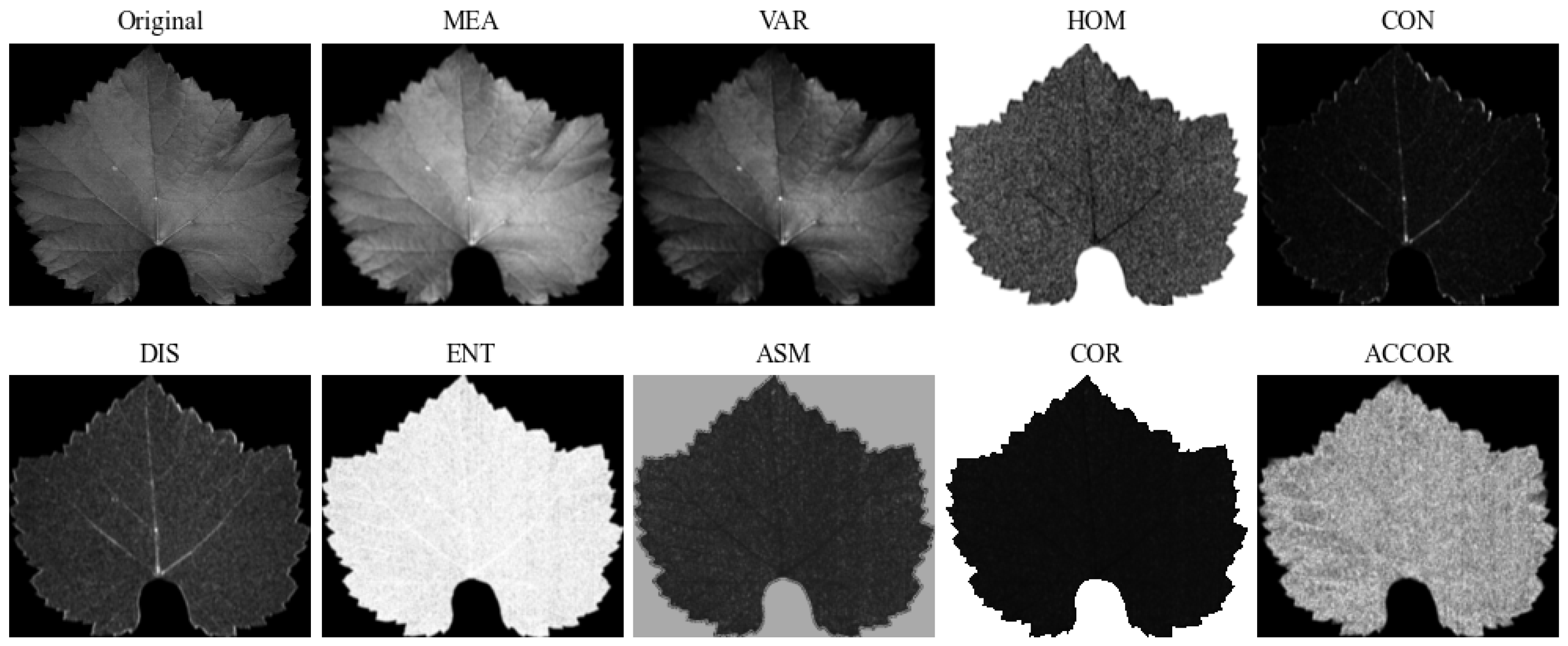
Plant texture features, both visual and tactile in nature, are often utilized as independent variables for phenotypic prediction [24]. In this study, we employed the gray-level co-occurrence matrix (GLCM) algorithm [25] to extract nine basic texture features: mean (MEA), variance (VAR), homogeneity (HOM), contrast (CON), dissimilarity (DIS), entropy (ENT), angular second moment (ASM), correlation (COR), and autocorrelation (ACOR). The mean feature values were computed across four orientations (0°, 45°, 90°, and 135°). Texture features were extracted from both RGB images with the background removed and hyperspectral images. To manage computational complexity, we selected five specific bands at 460, 550, 680, 750, and 916 nm, representing the blue, green, red, red-edge, and NIR bands, respectively. Texture was extracted from hyperspectral images following the approach described by Wang et al. [26]. Derived texture feature maps are presented in Figure 2.

2.4.4. Color Feature Extraction

Background information was removed from RGB images using matting software (accessed via: https://www.designkit.cn/cutout/, accessed on 10 December 2025). The hyperspectral images utilized for color feature extraction consisted of synthesized color images obtained from background-removed ROI images at 460, 550, and 680 nm. The average R, G, and B information of the region of interest was extracted using Python 3.11, and relevant color features were calculated according to the formulas shown in Table S2.

2.5. Regression Algorithm

Following the PLSR approach, a regression model is constructed by extracting principal components from independent variables that are strongly correlated with the dependent variables, combining the advantages of principal component analysis, canonical correlation analysis, and multiple linear regression to handle datasets with multicollinearity issues [27,28]. Gaussian process regression (GPR) is a Bayesian non-parametric method that utilizes kernel functions to model data similarity and capture nonlinear patterns [29]. Bayesian ridge regression (BRR) incorporates ridge regularization within a Bayesian framework to reduce model complexity, prevent overfitting, and provide uncertainty estimates for coefficients, which is especially useful when handling noisy or multicollinear data [30]. For all models, key parameters were optimized using five-fold cross-validation.

2.6. Model Performance Evaluation

The analytical framework integrated diverse features from hyperspectral and RGB sources: (a) spectral reflectance data, (b) vegetation indices, and (c) textural/color characteristics. During systematic classification, HSI-derived textural and color attributes were designated as HSI features, while their RGB-extracted counterparts were categorized as RGB features. The initial dimensionality of each feature category is detailed in Table 1.
Following feature extraction, all features were systematically integrated and transformed into one-dimensional feature vectors. The dataset was partitioned using a stratified random sampling approach, with 70% of samples allocated for model training and 30% for validation. During model development, the training subsets from all selected features were concatenated to form the composite training set. The corresponding test subsets were further combined to create the validation set, ensuring consistent evaluation across all feature types.
The analytical pipeline was executed using complementary software platforms: Python 3.11 was employed for data preparation, variable selection, color feature derivation, and predictive modeling, whereas texture features were computed in MATLAB R2022b. All regression models were developed using the sci-kit-learn machine learning library (version 1.2.2). The complete hyperparameters for each regression algorithm, including their numerical configurations, are detailed in Table S3.
K-fold cross-validation (K = 5) was performed for model optimization to minimize the coefficient of determination (R2) and identify optimum hyperparameter values. Z-score standardization was conducted on all predictor variables to promote consistent feature scales for model development and evaluation. All training and testing datasets underwent uniform preprocessing to ensure methodological consistency.
In this study, we examined four critical aspects for each model: (1) predictive accuracy, (2) measurement precision, (3) stability across trials, and (4) ability to estimate actual values. To quantitatively assess and compare the performance of different spectral parameters and modeling approaches, we used the following three established statistical metrics: (1) R2, (2) the normalized root mean square error (NRMSE), and (3) the relative percent difference (RPD). These metrics, whose mathematical formulations are provided in Table S4, collectively characterize the model’s predictive accuracy and robustness across varying conditions.

3. Results

3.1. Leaf Functional Traits

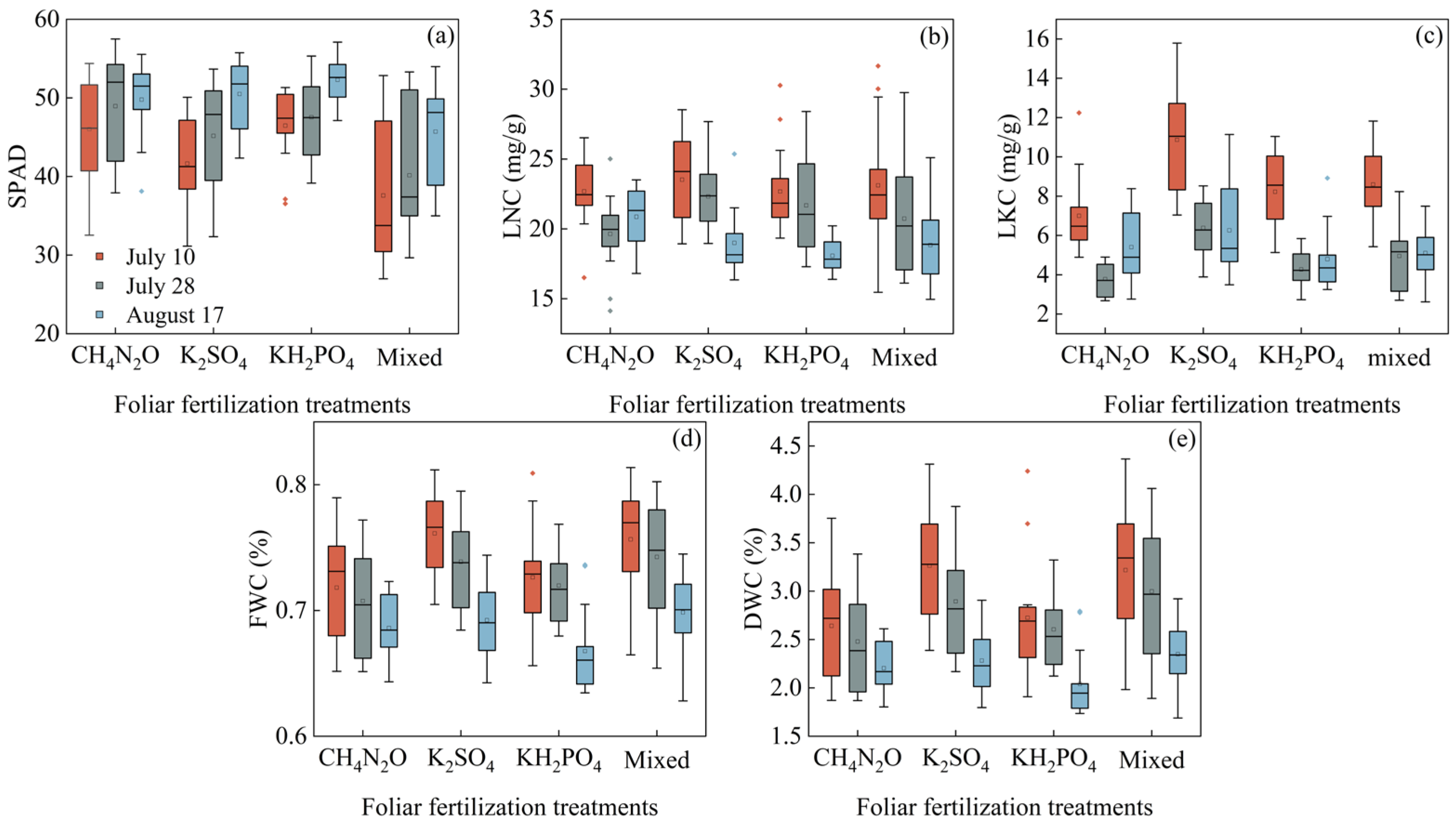
After foliar fertilization, the SPAD value rose with increasing fertilization frequency (Figure 3a), whereas FWC and DWC declined under greater fertilization frequency (Figure 3d,e). This suggests that repeated foliar spraying has a cumulative effect, enhancing chloroplast development and chlorophyll synthesis; moreover, repeated applications promote leaf growth, increase the accumulation of cell wall components such as cellulose and lignin, and consequently reduce the relative water content. Following the application of phosphorus, potassium, and mixed fertilizers, LNC exhibited a decreasing trend with increasing fertilization frequency (Figure 3b), which may be attributed to increased nitrogen consumption uptake driven by the stimulation of plant growth by phosphorus and potassium. When nitrogen fertilizer, phosphorus fertilizer, and mixed fertilizer were applied, LKC initially declined and subsequently increased (Figure 3c). This pattern may be explained by the high potassium demand during the rapid growth of new tissues, which results in the initial depletion of potassium [31]. Repeated application of external potassium resulted in accumulation, leading to a subsequent rebound in leaf potassium content.

3.2. Original Spectra

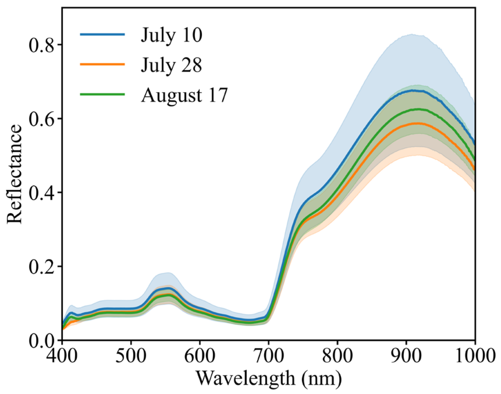
As shown in Figure 4, two notable reflectance peaks appeared in the spectral data at 550 nm (chlorophyll indicator) and 916 nm (water status marker) [32,33]. The spectra displayed several key features. In the visible range (400 to 500 nm), low reflectance values indicated strong light absorption by photosynthetic pigments. A distinct absorption feature occurred at 680 nm, corresponding to chlorophyll absorption maxima. Above 700 nm, the spectral reflectance rose sharply upon entering the NIR range, peaking at 916 nm due to intense scattering by foliar anatomical components. Although the reflectance slowly declined beyond 900 nm, persistently high values reflected the dual effects of cellular organization and hydration status [34].

3.3. Optimal Pretreatment Selection

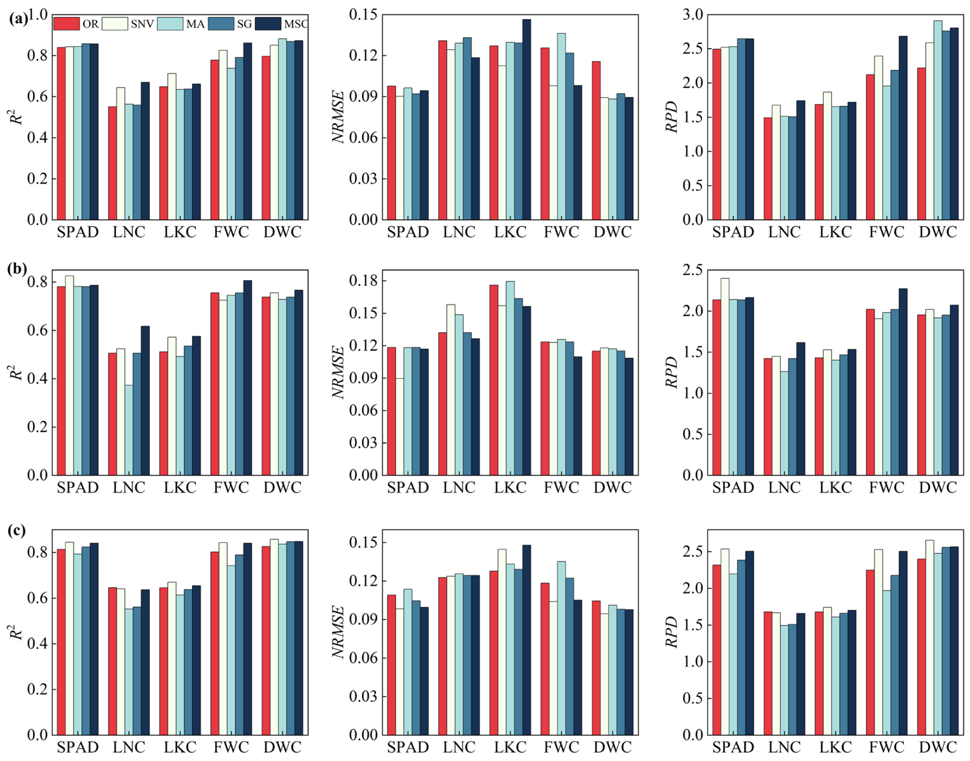
We developed predictive models for SPAD, LNC, LKC, FWC, and DWC utilizing three regression algorithms (PLSR, GPR, and BRR) applied to full-band spectra preprocessed using four methods (original spectra, SNV, MA, SG, and MSC). The comparative results (Figure 5, Tables S5–S7) revealed three key findings: (1) spectral preprocessing consistently enhanced model performance across all parameters; (2) scattering correction methods (SNV and MSC) generally outperformed smoothing techniques (MA and SG); and (3) the algorithms displayed a consistent performance hierarchy of PLSR > BRR > GPR.
The following optimal model configurations were identified: the SG-preprocessed PLSR model achieved superior performance for SPAD values (R2 = 0.8572, NRMSE = 0.092, RPD = 2.6461); the MSC-preprocessed model yielded optimal results for LNC (R2 = 0.67, NRMSE = 0.1185, RPD = 1.7408); the SNV-preprocessed model performed best for LKC (R2 = 0.7127, NRMSE = 0.1125, RPD = 1.8656); the MSC-preprocessed model showed the best accuracy for FWC measurement (R2 = 0.8611, NRMSE = 0.0981, RPD = 2.6833); and the MA-preprocessed model demonstrated the highest precision for DWC assessment (R2 = 0.8819, NRMSE = 0.0882, RPD = 2.9099). Based on these findings, subsequent analyses were conducted using the optimal preprocessing method for each parameter.

3.4. Feature Selection

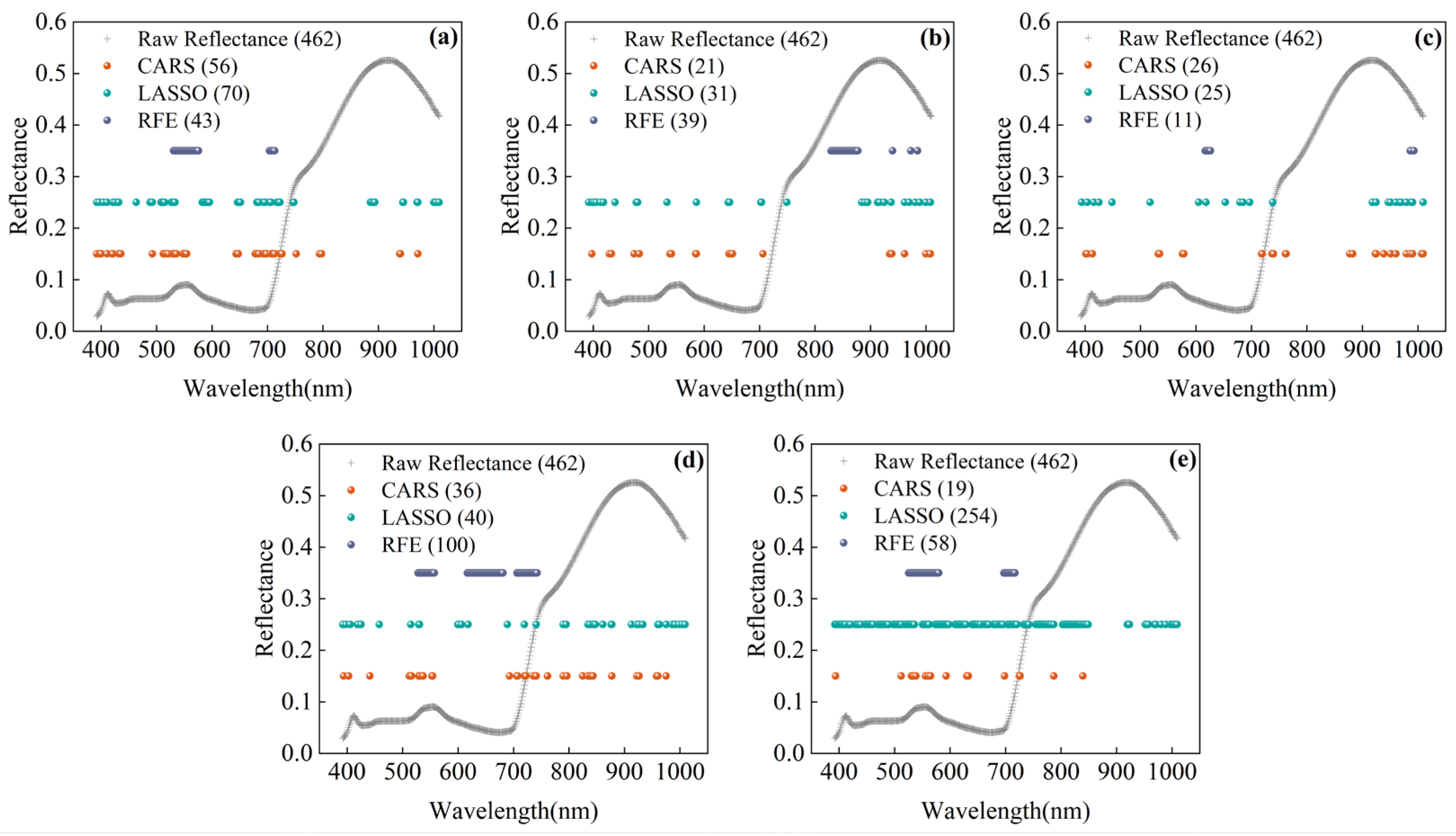
Feature selection is crucial for mitigating data redundancy and enhancing both the accuracy and robustness of predictive models. The present study demonstrates the advantages of establishing comprehensive predictive models through the application of preprocessing techniques. Employing methods including CARS, LASSO, and RFE, we selected characteristic wavelengths from the optimally preprocessed full-spectrum reflectance data based on various physicochemical indices. The selected feature wavelengths are presented in Figure 6a–e). CARS and LASSO exhibited partial overlap in the wavelengths selected for the same physicochemical values, whereas RFE yielded a more concentrated selection. Compared with the full-spectrum data, which comprised 462 bands, feature selection using different algorithms significantly reduced the number of retained wavelengths. Specifically, the number of wavelengths selected by CARS decreased by over 87%; the application of LASSO reduced the number of wavelengths by over 45%; and RFE eliminated more than 78% of wavelengths.
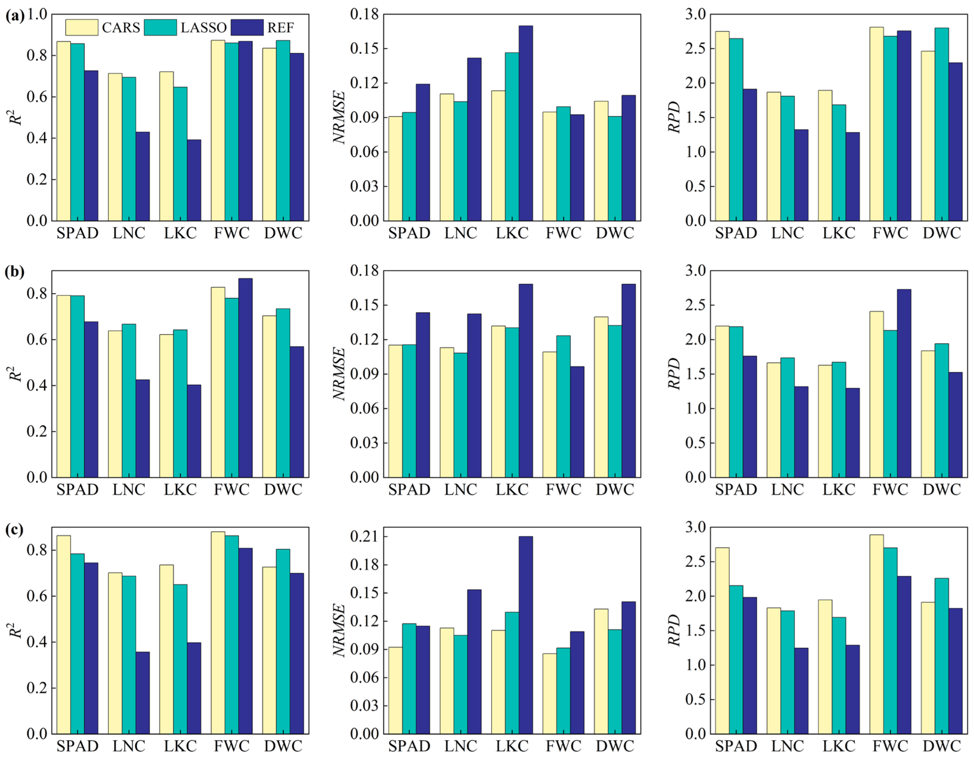
To further enhance the predictive accuracy of the models for grapevine leaf functional traits, the selected characteristic wavelengths were integrated as inputs into regression models. The predictive performance of these models, including PLS, GPR, and BRR, for various grapevine leaf functional traits is presented in Figure 7 (detailed values are provided in Tables S8–S10). Following feature wavelength selection, most models displayed improved performance. The optimal preprocessing methods and feature wavelength selection techniques for each indicator are detailed in Table 2. CARS demonstrated superior performance in predicting SPAD, LNC, LKC, and FWC, with improvements observed after feature wavelength selection compared with the full-spectrum models. Among the three feature selection models, the LASSO algorithm performed the best in DWC prediction; however, its performance decreased relative to the full-band prediction model. This aligns with the findings of Curran et al. [35], suggesting that feature selection methods can often neglect the spectral characteristics of dry matter. Therefore, for SPAD, LNC, LKC, and FWC, the wavelength after optimal preprocessing and CARS feature selection was selected as the Ref of the feature combination, while the reflectance after MA preprocessing was used as the Ref for DWC.

3.5. Correlation Analysis of Relationships Between Different Features and Leaf Functional Traits

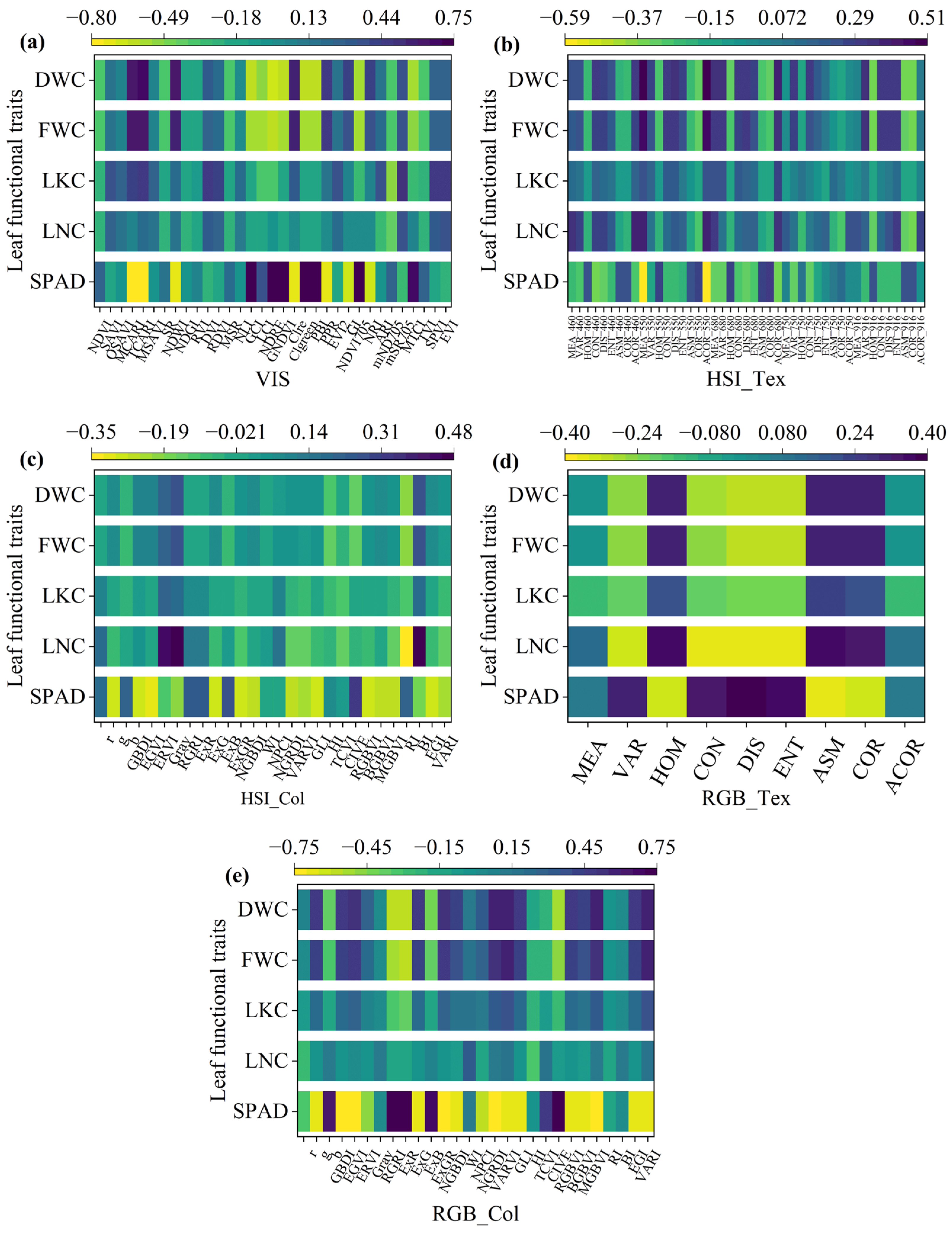
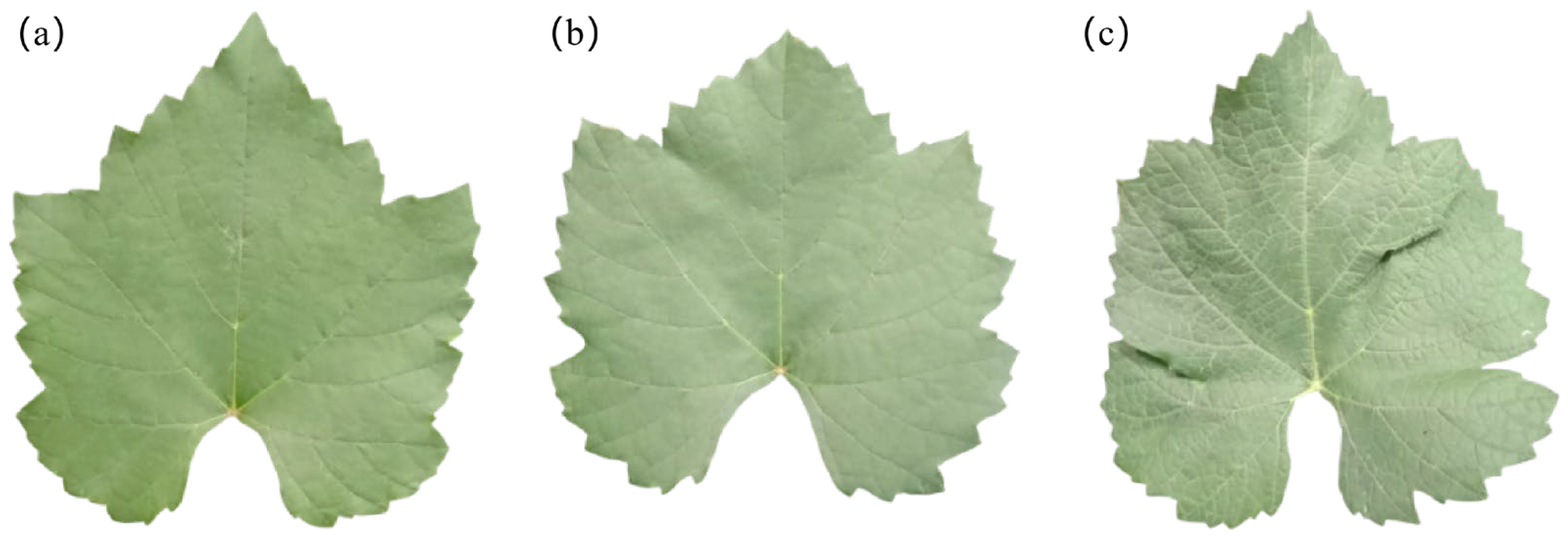
Correlation analysis was conducted between various vegetation indices, hyperspectral, and RGB image color and texture features with grapevine leaf functional traits. According to the Pearson correlation coefficient significance thresholds [36], with a sample size of n = 180, |r| > 0.145 indicated significance at the 0.05 level, |r| > 0.19 reflected significance at the 0.01 level, and |r| > 0.242 showed significance at the 0.001 level. Table 3 presents the number of features displaying significant correlations (p < 0.01) with each index, and the Pearson correlation coefficient plots between parameters and grapevine leaf traits are shown in Figure 8. The results indicated that among the various indices, correlations with SPAD values were relatively higher, whereas those with LNC and LKC were comparatively weaker, likely due to the direct optical signals of nitrogen and potassium deficiencies and their limited effect on leaf structure. Notably, vegetation indices exhibited the strongest correlations with the parameters of SPAD, LKC, FWC, and DWC, with correlation coefficients of −0.79, −0.53, 0.64, and 0.68, respectively. Vegetation indices derived from combined peaks (550 nm and 916 nm) and troughs (680 nm and 705 nm) revealed particularly strong associations. Color features from hyperspectral data showed the strongest correlation with LNC, with a coefficient of 0.47. As shown in Table 3, features related to SPAD were more numerous. RGB images corresponding to different SPAD values are presented in Figure 9, illustrating that leaf coloration intensifies as SPAD values increase.

3.6. Performance of Feature Combination Leaf Functional Traits

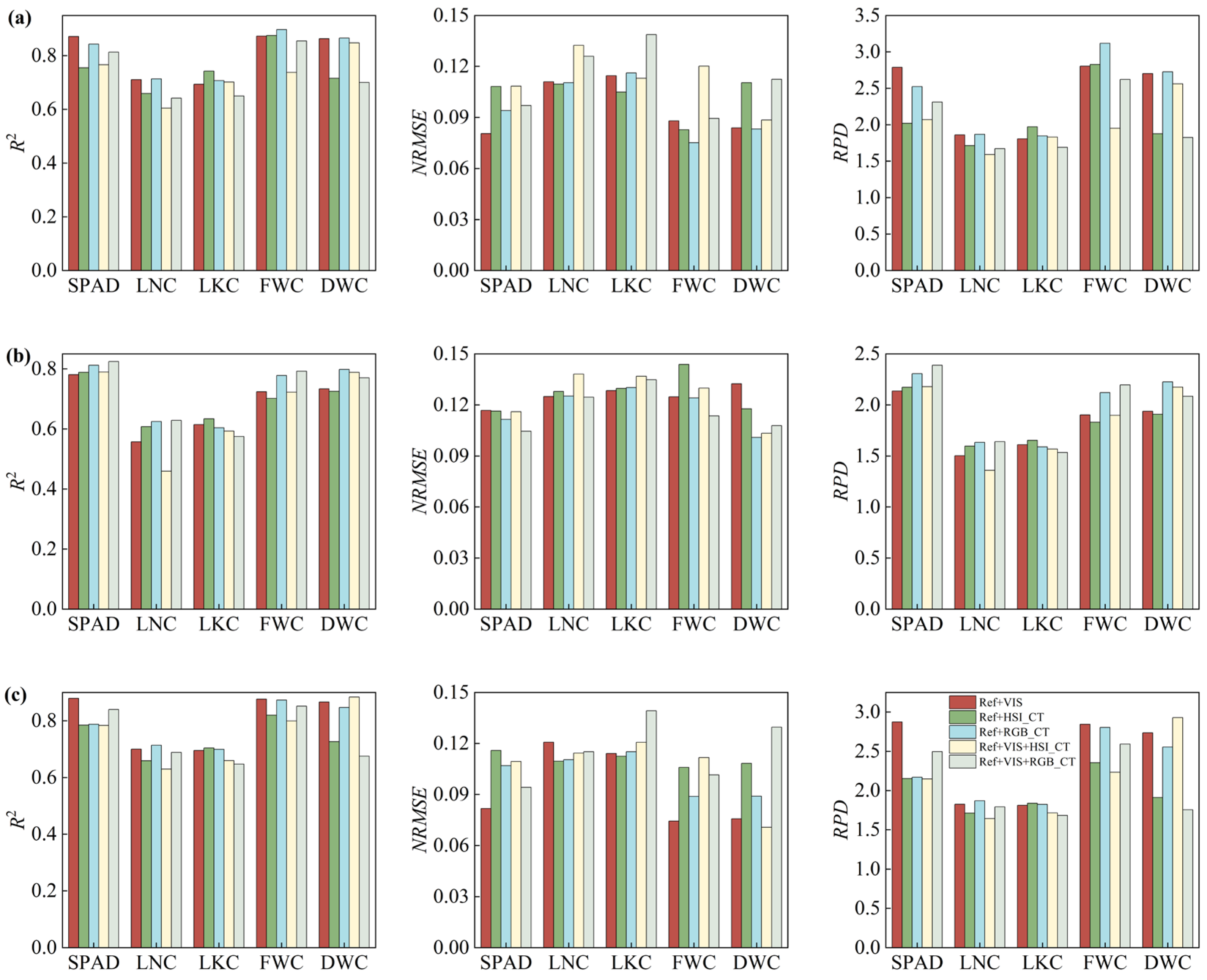
To confirm that the leaf trait prediction accuracy was improved by including VIS, HSI_CT, and RGB_CT features, we further incorporated the features that displayed a significant correlation with each trait. Previous research demonstrated that feature combinations could yield superior predictive performance [12]; therefore, in the present study, we did not model individual features separately. Five combination schemes were tested: Ref + VIS, Ref + HSI_CT, Ref + RGB_CT, Ref + VIS + HSI_CT, and Ref + VIS + RGB_CT. The performance of these models with different feature combinations is illustrated in Figure 10, with detailed values provided in Tables S11–S13. For the same leaf trait, model performance across different feature combinations was generally consistent. Among the models, PLSR and BRR outperformed GPR in terms of predictive accuracy.
Ref + VIS performed well in SPAD prediction, and the BRR model showed the best performance with R2, NRMSE, and RPD values of 0.8790, 0.0818, and 2.8744, respectively. This may be because vegetation indices integrate multiple spectral bands, thereby providing more stability than single wavelengths. Ref + RGB_CT demonstrated superior predictive ability for LNC and FWC, with BRR and PLSR achieving the best R2 values at 0.7137 and 0.8970, respectively. This indicates that RGB image features can partially reflect leaf nitrogen and water content. Ref + HSI_CT performed well in predicting LKC, with the optimal model being PLSR, yielding R2, NRMSE, and RPD values of 0.7426, 0.1049, and 1.9709, respectively. Compared with the raw spectra, R2 and RPD increased by 14.55% and 16.88%, respectively, while NRMSE declined by 18.24%. This improvement may be attributed to the higher spatial resolution of hyperspectral images, which helps capture subtle morphological variations, thereby enhancing the accuracy of LKC prediction. For DWC prediction, the BRR model combined with Ref + VIS + HSI_CT performed best, obtaining R2, NRMSE, and RPD values of 0.8834, 0.0707, and 2.9285, respectively. Correlation analysis revealed that all features had maximum correlations with DWC exceeding 0.5. This indicates that this feature combination enables models to effectively utilize data complexity without overfitting, thereby enhancing model performance.
Additionally, the GPR model performed well in SPAD, LNC, and FWC prediction within the Ref + VIS + RGB_CT feature set. The GPR model may leverage kernel functions to learn more complex nonlinear relationships, giving it an advantage in multi-feature models. However, not all feature sets enhanced leaf trait prediction; in some cases, model performance declined, likely due to feature redundancy or the manner of feature combination.

4. Discussion

4.1. Contribution of Feature Types to Leaf Trait Prediction

Integrating diverse feature types enhances the prediction of grape leaf traits. Correlation analysis indicates significant differences in the predictive potential of vegetation indices for various leaf functional traits. Specifically, vegetation indices exhibit the strongest correlation with SPAD values (|r|max = 0.79), primarily because most VIS utilize a combination of the red light band (680 nm), where chlorophyll absorption is intense, and the near-infrared band, characterized by strong structural reflectance from leaves, effectively amplifying chlorophyll spectral signals [37]. Similarly, VIS demonstrates notable correlations with both FWC and DWC, with maximum correlation coefficients of 0.64 and 0.68, respectively, as many VIS are sensitive to water absorption bands in the near-infrared region (e.g., 970 nm), thereby indirectly reflecting water status [38]. Conversely, the correlations between VIS and LNC and LKC are comparatively weaker (|r|max = 0.40 and 0.53). This is due to the absence of distinct spectral absorption features for nitrogen and potassium; their spectral signals are typically mediated indirectly through impacts on chlorophyll synthesis and leaf structural properties, adding complexity and making direct estimation more challenging [39].
A comparison of feature types revealed clear performance differences. Hyperspectral texture features exhibited stronger leaf trait correlations than RGB-based features, likely because they better captured fine-scale leaf surface structures and tissue organization. This advantage stemmed from HSI’s high spectral resolution, which allowed for a more precise analysis of microstructural–spectral relationships [40]. Conversely, RGB color features displayed stronger correlations than their hyperspectral counterparts. This is because RGB values directly represent leaf surface coloration—a visible indicator of underlying physiological status [41].
Furthermore, in this study, textural features were extracted from hyperspectral images at only five wavebands (460, 550, 680, 750, and 916 nm), while three wavebands (460, 550, and 680 nm) were employed for color feature extraction. Future research could explore the use of other band combinations for the extraction of color features from hyperspectral images.

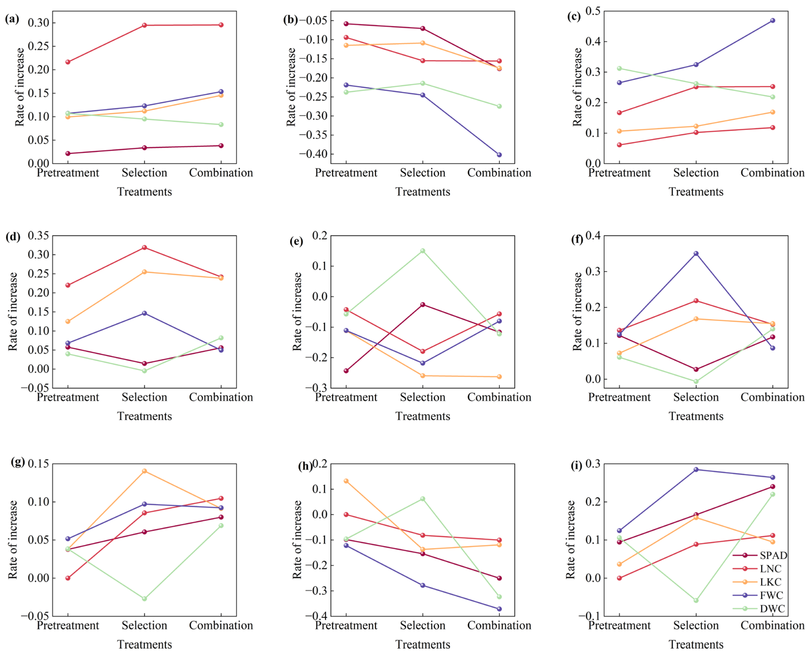
4.2. Effect of Different Optimization Methods on Model Performance

Variations in model performance with respect to optimal preprocessing, feature selection, and feature combination methods across different models are illustrated in Figure 11. After preprocessing, the performance of most models improved across various metrics. The R2 value for PLSR increased by 2.14–21.64%, that of GPR rose by 3.97–22%, and that of BRR increased by 0–5.16%. This indicates that the selected preprocessing techniques effectively enhance data quality by mitigating scattering and noise, consistent with the findings of Guo et al. [42]. Following feature selection, all models showed performance improvements compared with the original spectral feature selection method, with increases in R2 and RPD values and reductions in NRMSE, except for the GPR and BRR models in the prediction of DWC. The R2 value for PLSR increased by 3.38–29.48%, that of GPR rose by −0.47–31.9%, and that of BRR increased by −2.71–14.04%. After feature combination, the performance metrics of all models improved relative to the original spectral data, with the R2 value for PLSR increasing by 3.83–29.56%, that of GPR increasing by 4.95–24.17%, and that of BRR increasing by 6.88–10.46%.
PLSR demonstrates a highly consistent and positive response to multi-stage collaborative optimization strategies, with the model showing progressive performance improvements across most traits, except for DWC. The feature selection process for DWC was relatively complex, resulting in an inconspicuous effect of feature selection on its role within the model. In GPR models, performance fluctuates with trait specificity primarily because Gaussian Process Regression captures nonlinear relationships through kernel functions. However, it is sensitive to feature dimensionality and noise, especially when the sample size is limited. In the GPR model, the performance improved after feature selection for LNC, LKC, and FWC, demonstrating the effectiveness of CARS feature selection. Conversely, model performance declined for other indicators after feature selection, possibly because CARS is based on PLSR feature selection, which tends to perform better in linear models [43]. Future research could explore alternative feature screening methods. In the BRR model, all optimization techniques enhanced the prediction of SPAD and LNC, with stepwise improvement in model performance. However, the predictive performance of LKC and FWC declined after feature combination. This was likely due to the increased number of features, which may have weakened the regularization effect of BRR and thus reduced model performance, as confirmed by Sahebalam et al. [44]. After feature selection, the model performance for DWC was reduced relative to the original spectra, suggesting that LASSO feature selection may have eliminated key spectral bands. Future studies could further investigate the effect of different feature combination sequences on model performance.
Overall, the performance enhancement hierarchy was found to be GPR > PLSR > BRR, indicating that GPR may capture more complex nonlinear relationships through feature combination. This corresponds with the findings of Duvenaud et al., suggesting that feature integration is more suitable for GPR’s nonlinear modeling capabilities [45]. Regarding modeling effectiveness, feature selection outperformed feature combination and preprocessing, demonstrating that combining these techniques can optimize predictive accuracy, consistent with the results of Xie et al. [46]. LNC prediction showed the most significant enhancement after optimization, while the enhancements in SPAD and DWC prediction were relatively smaller. These outcomes are presumably attributable to the intrinsic characteristics of these indicators, such as data noise levels and feature correlations, corroborating the findings of Luo et al. [9].

4.3. Characteristics of Regression Algorithms in Leaf Trait Prediction

In this study, we employed two linear regression models and a single nonlinear regression model to address high-dimensional, small-sample-size data. The results showed that PLSR and BRR were more stable, and linear regression modeling exhibited better performance in addressing single-source data and high-correlation features with target values, which was consistent with the results of Burnett et al. [27]. In this study, the performance of GPR was relatively poor for small-sample-size data, although GPR performed well with the utilization of multi-feature combinations. Moreover, the sample size can be further increased to enhance the GPR model’s accuracy.
These findings offer valuable guidance for model selection in spectroscopic applications, particularly when dealing with the issues of high-dimensional, small-sample data, which are prevalent in plant phenotyping research. The comparison suggests that model performance is related to both data characteristics (dimensionality, sample size, and correlations among features) and inherent model characteristics (linearity assumptions and parameter estimation requirements) [47].

5. Conclusions

In this study, a multi-stage cooperative optimization framework was developed. The effects of various preprocessing methods, feature selection techniques, and feature combinations on the prediction of functional traits in grapevine leaves were analyzed. The results indicated that incorporating different data processing approaches can effectively enhance the predictive performance of various models for grapevine leaf functional traits. Notably, CARS outperformed the other two feature selection methods in predicting SPAD, LNC, LKC, and FWC, reducing the number of wavelengths by 87% and achieving optimal model performance. Comparative analysis revealed that the Gaussian Process Regression (GPR) model demonstrated the greatest potential for performance improvement through optimization, with feature selection emerging as the most influential stage within this framework. The multi-stage collaborative optimization framework developed in this study significantly improves the accuracy of predicting grape leaf functional traits and provides a theoretical foundation for future research. Subsequent studies should focus on validating and expanding this framework by incorporating larger, more diverse datasets, including different grape varieties, environmental conditions, and growth stages. Additionally, exploring a broader range of hyperspectral bands for texture and color feature extraction could further unlock the potential of image-based phenotyping.

Supplementary Materials

The following supporting information can be downloaded at: https://www.mdpi.com/article/10.3390/agronomy16010029/s1. Table S1. Collected hyperspectral vegetation indices in this study. Table S2. Color features extracted from RGB and hyperspectral images in this study. Table S3. Hyperparameters in the selected regression algorithms. Table S4. Introduction to model performance indicators. Table S5. The prediction results of the PLSR model for the functional traits of grape leaves under different pretreatments. Table S6. The prediction results of the GPR model for the functional traits of grape leaves under different pretreatments. Table S7. The prediction results of the BRR model for the functional traits of grape leaves under different pretreatments. Table S8. The prediction results of the PLSR model for functional traits of grape leaves under different feature selections. Table S9. The prediction results of the GPR model for functional traits of grape leaves under different feature selections. Table S10. The prediction results of the BRR model for functional traits of grape leaves under different feature selections. Table S11. The prediction results of the PLSR model for the functional traits of grape leaves under different feature combinations. Table S12. The prediction results of the GPR model for the functional traits of grape leaves under different feature combinations. Table S13. The prediction results of the BRR model for the functional traits of grape leaves under different feature combinations. References [48,49,50,51,52,53,54,55,56,57,58,59,60,61,62,63,64,65,66,67,68,69,70,71,72,73,74,75,76,77,78,79,80,81,82,83,84,85,86,87,88] have been mentioned in the text.

Author Contributions

Research design and data collection: Q.J., K.L. and Z.W.; Data analysis and interpretation: Q.J., X.Z. and W.L.; Drafting of the manuscript: Q.J.; Major revisions and final approval: Q.J., X.Z., K.L., Z.W., Y.S., K.H., Y.F., X.S. and W.L.; The conception and design of the study & research support and guidance: W.L. All authors have read and agreed to the published version of the manuscript.

Funding

This work was supported by the National Natural Science Foundation of China [32201678], the Key R&D Program of Shandong Province, China [2023TZXD062], and the Key R&D Program of Shanxi Province, China [2025NC-YBXM-219].

Data Availability Statement

The data supporting this study are included within the article and/or Supplementary Materials.

Conflicts of Interest

The authors declare that they have no known competing financial interests or personal relationships that could have appeared to influence the work reported in this paper.

References

  1. Jetz, W.; Cavender-Bares, J.; Pavlick, R.; Schimel, D.; Davis, F.W.; Asner, G.P.; Guralnick, R.; Kattge, J.; Latimer, A.M.; Moorcroft, P. Monitoring plant functional diversity from space. Nat. Plants 2016, 2, 16024. [Google Scholar] [CrossRef]
  2. Bruelheide, H.; Dengler, J.; Purschke, O.; Lenoir, J.; Jiménez-Alfaro, B.; Hennekens, S.M.; Botta-Dukát, Z.; Chytry, M.; Field, R.; Jansen, F.; et al. Global trait-environment relationships of plant communities. Nat. Ecol. Evol. 2018, 2, 1906–1917. [Google Scholar] [CrossRef]
  3. Li, X.Y.; Liu, Y.M.; Wang, H.Y.; Dong, X.Z.; Wang, L.; Long, Y.Q. Comparing Stacking Ensemble Learning and 1D-CNN Models for Predicting Leaf Chlorophyll Content in Stellera chamaejasme from Hyperspectral Reflectance Measurements. Agriculture 2025, 15, 288. [Google Scholar] [CrossRef]
  4. Liu, N.; Wagner, H.E.; Hansen, N.T.P.A. Multi-year hyperspectral remote sensing of a comprehensive set of crop foliar nutrients in cranberries. ISPRS J. Photogramm. Remote Sens. 2023, 205, 135–146. [Google Scholar] [CrossRef]
  5. Lin, W.; Li, Y.; Du, S.; Zheng, Y.; Gao, J.; Sun, T. Effect of dust deposition on spectrum-based estimation of leaf water content in urban plant. Ecol. Indic. 2019, 104, 41–47. [Google Scholar] [CrossRef]
  6. Correspondence, J.; Kattge, J.; Bnisch, G.; Diaz, S.; Wirth, C. TRY plant trait database—enhanced coverage and open access. Glob. Change Biol. 2020, 26, 119–188. [Google Scholar] [CrossRef]
  7. Pan, W.; Cheng, X.; Du, R.; Zhu, X.; Guo, W. Detection of chlorophyll content based on optical properties of maize leaves. Spectrochim. Acta Part A Mol. Biomol. Spectrosc. 2024, 309, 123843. [Google Scholar] [CrossRef] [PubMed]
  8. Watt, M.S.; Buddenbaum, H.; Leonardo, E.M.C.; Estarija, H.J.C.; Bown, H.E.; Gomez-Gallego, M.; Hartley, R.; Massam, P.; Wright, L.; Zarco-Tejada, P.J. Using hyperspectral plant traits linked to photosynthetic efficiency to assess N and P partition. ISPRS J. Photogramm. Remote Sens. 2020, 169, 406–420. [Google Scholar] [CrossRef]
  9. Luo, Q.; Tang, T.; Duan, Y.X.; Li, J.L.; Ling, C.J.; Gao, T.; Wu, W.B. Nitrogen-phosphorus responses and Vis/NIR prediction in fresh tea leaves. Food Chem. 2025, 476, 143369. [Google Scholar] [CrossRef] [PubMed]
  10. Azadnia, R.; Rajabipour, A.; Jamshidi, B.; Omid, M. New approach for rapid estimation of leaf nitrogen, phosphorus, and potassium contents in apple-trees using Vis/NIR spectroscopy based on wavelength selection coupled with machine learning. Comput. Electron. Agric. 2023, 207, 16. [Google Scholar] [CrossRef]
  11. Li, Y.F.; Xu, X.A.; Wu, W.B.; Zhu, Y.H.; Gao, L.T.; Jiang, X.T.; Meng, Y.; Yang, G.J.; Xue, H.Y. Hyperspectral estimation of chlorophyll content in grapevine based on feature selection and GA-BP. Sci. Rep. 2025, 15, 13. [Google Scholar] [CrossRef]
  12. Ma, L.F.; Li, Y.J.; Yuan, N.G.; Liu, X.J.; Yan, Y.Y.; Zhang, C.R.; Fang, S.H.; Gong, Y. The Inversion of Rice Leaf Pigment Content: Using the Absorption Spectrum to Optimize the Vegetation Index. Agriculture 2024, 14, 2265. [Google Scholar] [CrossRef]
  13. Jiao, Z.J.; Zhang, Z.M.; Zhang, A.Z.; Sun, G.Y.; Wu, L.X. Modified Multiple Spectrum-Based Vegetation Index (MMSVI): A Reflectance Index With High Spatiotemporal Generalization Ability. IEEE Trans. Geosci. Remote Sens. 2024, 62, 13. [Google Scholar] [CrossRef]
  14. Yang, Z.; Tian, J.; Feng, K.; Gong, X.; Liu, J. Application of a hyperspectral imaging system to quantify leaf-scale chlorophyll, nitrogen and chlorophyll fluorescence parameters in grapevine. Plant Physiol. Biochem. 2021, 166, 723–737. [Google Scholar] [CrossRef]
  15. Chen, D.S.; Zhang, F.; Tan, M.L.; Chan, N.W.; Shi, J.C.; Liu, C.J.; Wang, W.W. Improved Na+ estimation from hyperspectral data of saline vegetation by machine learning. Comput. Electron. Agric. 2022, 196, 13. [Google Scholar] [CrossRef]
  16. Ma, H.; Zhao, W.; Yu, H.; Yang, P.; Yang, F.; Li, Z. Diagnosis alfalfa salt stress based on UAV multispectral image texture and vegetation index. Plant Soil 2024, 513, 585–603. [Google Scholar] [CrossRef]
  17. Sadeghi, A.; Khani, S.; Sabourian, R.; Hajimahmoodi, M.; Ghasemi, J.B. Integrating CNNs and chemometrics for analyzing NIR spectra and RGB images in turmeric adulterant detection. J. Food Compos. Anal. 2025, 141, 107324. [Google Scholar] [CrossRef]
  18. Ali, M.M.E.; Petropoulos, S.A.; Selim, D.; Elbagory, M.; Othman, M.M.; Omara, A.E.; Mohamed, M.H. Plant Growth, Yield and Quality of Potato Crop in Relation to Potassium Fertilization. Agronomy 2021, 11, 675. [Google Scholar] [CrossRef]
  19. Guo, J.M.; Huang, H.; He, X.L.; Cai, J.W.; Zeng, Z.X.; Ma, C.Y.; Lü, E.L.; Shen, Q.Y.; Liu, Y.H. Improving the detection accuracy of the nitrogen content of fresh tea leaves by combining FT-NIR with moisture removal method. Food Chem. 2023, 405, 8. [Google Scholar] [CrossRef]
  20. Feng, C.H.; Otani, C.; Ogawa, Y. Innovatively identifying naringin and hesperidin by using terahertz spectroscopy and evaluating flavonoids extracts from waste orange peels by coupling with multivariate analysis. Food Control 2022, 137, 108897. [Google Scholar] [CrossRef]
  21. Ouyang, Q.; Wang, L.; Park, B.; Kang, R.; Chen, Q. Simultaneous quantification of chemical constituents in matcha with visible-near infrared hyperspectral imaging technology. Food Chem. 2021, 350, 129141. [Google Scholar] [CrossRef] [PubMed]
  22. Al-Mbaideen, A.A. Application of Moving Average Filter for the Quantitative Analysis of the NIR Spectra. J. Anal. Chem. 2019, 74, 686–692. [Google Scholar] [CrossRef]
  23. Mirzaie, M.; Darvishzadeh, R.; Shakiba, A.; Matkan, A.A.; Atzberger, C.; Skidmore, A. Comparative analysis of different uni- and multi-variate methods for estimation of vegetation water content using hyper-spectral measurements (vol 26, pg 1, 2014). Int. J. Appl. Earth Obs. Geoinf. 2014, 28, 260. [Google Scholar] [CrossRef]
  24. Liu, X.; Du, R.Q.; Xiang, Y.Z.; Chen, J.Y.; Zhang, F.C.; Shi, H.Z.; Tang, Z.J.; Wang, X. Estimating Winter Canola Aboveground Biomass from Hyperspectral Images Using Narrowband Spectra-Texture Features and Machine Learning. Plants 2024, 13, 2978. [Google Scholar] [CrossRef]
  25. Zhu, F.; Wei, H.; Shen, Y.; Zhang, Y.; Xu, N.; Zheng, H.; Qiao, X.; Liu, D. A multi-feature fusion based method for detecting the moisture content of withered black tea. J. Food Compos. Anal. 2025, 141, 107325. [Google Scholar] [CrossRef]
  26. Wang, D.; Struik, P.C.; Liang, L.; Yin, X.Y. Estimating leaf and canopy nitrogen contents in major field crops across the growing season from hyperspectral images using nonparametric regression. Comput. Electron. Agric. 2025, 233, 14. [Google Scholar] [CrossRef]
  27. Burnett, A.C.; Jeremiah, A.; Davidson, K.J.; Ely, K.S.; Julien, L.; Qianyu, L.; Morrison, B.D.; Dedi, Y.; Alistair, R.; Serbin, S.P. A best-practice guide to predicting plant traits from leaf-level hyperspectral data using partial least squares regression. J. Exp. Bot. 2021, 72, 6175–6189. [Google Scholar] [CrossRef]
  28. Wang, Z.; Bureau, S.; Jaillais, B.; Renard, C.M.G.C.; Chen, X.; Sun, Y.; Lv, D.; Pan, L.; Lan, W. Infrared guided smart food formulation: An innovative spectral reconstruction strategy to develop anticipated and constant apple puree products. Food Innov. Adv. 2024, 3, 20. [Google Scholar] [CrossRef]
  29. Xie, R.; Darvishzadeh, R.; Skidmore, A.K.; Heurich, M.; Holzwarth, S.; Gara, T.W.; Reusen, I. Mapping leaf area index in a mixed temperate forest using Fenix airborne hyperspectral data and Gaussian processes regression. Int. J. Appl. Earth Obs. Geoinf. 2021, 95, 13. [Google Scholar] [CrossRef]
  30. Huang, Y.; Chen, Z.; Liu, J. Near-infrared spectral expansion method based on active semi-supervised regression. Anal. Chim. Acta 2024, 1317, 342890. [Google Scholar] [CrossRef] [PubMed]
  31. Tao, J.; Liu, X. Combined application of nitrogen and phosphorus fertilizers increases soil organic carbon storage in cropland soils. Eur. J. Agron. 2025, 168, 127607. [Google Scholar] [CrossRef]
  32. Gai, J.; Wang, J.; Xie, L.W.; Xiang, L.; Wang, Z. Spectroscopic determination of chlorophyll content in sugarcane leaves for drought stress detection. Precis. Agric. 2024, 25, 543–569. [Google Scholar] [CrossRef]
  33. Dou, S.; Zhang, W.; Deng, Y.; Zhang, C.; Mei, Z.; Yan, J.; Li, M. Comparison of Citrus Leaf Water Content Estimations Based on the Continuous Wavelet Transform and Fractional Derivative Methods. Horticulturae 2024, 10, 177. [Google Scholar] [CrossRef]
  34. Li, C.; Xiao, Z.; Liu, Y.; Meng, X.; Li, X.; Wang, X.; Li, Y.; Zhao, C.; Ren, L.; Yang, C. Hyperspectral Estimation of Winter Wheat Leaf Water Content Based on Fractional Order Differentiation and Continuous Wavelet Transform. Agronomy 2022, 13, 56. [Google Scholar] [CrossRef]
  35. Curran, P.J. Remote sensing of foliar chemistry. Remote Sens. Environ. 1990, 30, 271–278. [Google Scholar] [CrossRef]
  36. Fan, J.; Wang, H.; Liao, Z.; Dai, Y.; Yu, J.; Feng, H. Winter Wheat Leaf Area Index Estimation Based on Texture-color Features and Vegetation Indices. J. China Agric. Univ. 2023, 54, 7. (In Chinese) [Google Scholar] [CrossRef]
  37. Parida, P.K.; Somasundaram, E.; Krishnan, R.; Radhamani, S.; Sivakumar, U.; Parameswari, E.; Raja, R.; Rangasami, S.R.S.; Sangeetha, S.P.; Selvi, R.G. Unmanned Aerial Vehicle-Measured Multispectral Vegetation Indices for Predicting LAI, SPAD Chlorophyll, and Yield of Maize. Agriculture 2024, 14, 1110. [Google Scholar] [CrossRef]
  38. Casas, A.; Riaño, D.; Ustin, S.L.; Dennison, P.; Salas, J. Estimation of water-related biochemical and biophysical vegetation properties using multitemporal airborne hyperspectral data and its comparison to MODIS spectral response. Remote Sens. Environ. 2014, 148, 28–41. [Google Scholar] [CrossRef]
  39. Zhang, Y.; Xiao, J.; Yan, K.; Lu, X.; Li, W.; Tian, H.; Wang, L.; Deng, J.; Lan, Y. Advances and Developments in Monitoring and Inversion of the Biochemical Information of Crop Nutrients Based on Hyperspectral Technology. Agronomy 2023, 13, 2163. [Google Scholar] [CrossRef]
  40. Deng, X.; Lan, Y.; Hong, T.; Chen, J. Citrus greening detection using visible spectrum imaging and C-SVC. Comput. Electron. Agric. 2016, 130, 177–183. [Google Scholar] [CrossRef]
  41. Wang, X.L.; Li, J.Q.; Zhang, J.Q.; Yang, L.; Cui, W.H.; Han, X.W.; Qin, D.L.; Han, G.T.; Zhou, Q.; Wang, Z.S.; et al. Estimation of Cotton SPAD Based on Multi-Source Feature Fusion and Voting Regression Ensemble Learning in Intercropping Pattern of Cotton and Soybean. Agronomy 2024, 14, 2245. [Google Scholar] [CrossRef]
  42. Guo, Z.; Jayan, H. Fast Nondestructive Detection Technology and Equipment for Food Quality and Safety. Foods 2023, 12, 3744. [Google Scholar] [CrossRef] [PubMed]
  43. Li, H.; Liang, Y.; Xu, Q.; Cao, D. Key wavelengths screening using competitive adaptive reweighted sampling method for multivariate calibration. Anal. Chim. ACTA 2009, 648, 77–84. [Google Scholar] [CrossRef]
  44. Sahebalam, H.; Gholizadeh, M.; Hafezian, H. Investigating the Performance of Frequentist and Bayesian Techniques in Genomic Evaluation. Biochem. Genet. 2025, 63, 3240–3266. [Google Scholar] [CrossRef]
  45. Duvenaud, D.; Lloyd, J.R.; Grosse, R.; Tenenbaum, J.B.; Ghahramani, Z. Structure Discovery in Nonparametric Regression through Compositional Kernel Search. In OTM Confederated International Conferences “On the Move to Meaningful Internet Systems”; Springer: Berlin/Heidelberg, Germany, 2013. [Google Scholar] [CrossRef]
  46. Xie, J.; Wang, J.; Chen, Y.; Gao, P.; Yin, H.; Chen, S.; Sun, D.; Wang, W.; Mo, H.; Shen, J. Estimating the SPAD of Litchi in the Growth Period and Autumn Shoot Period Based on UAV Multi-Spectrum. Remote Sens. 2023, 15, 5767. [Google Scholar] [CrossRef]
  47. Maimaitijiang, M.; Sagan, V.; Sidike, P.; Hartling, S.; Fritschi, F.B. Soybean yield prediction from UAV using multimodal data fusion and deep learning. Remote Sens. Environ. 2019, 237, 111599. [Google Scholar] [CrossRef]
  48. Tucker, C.J. Red and photographic infrared linear combinations for monitoring vegetation. Remote Sens. Environ. 1979, 8, 127–150. [Google Scholar] [CrossRef]
  49. Huete, A.R.; Liu, H.Q.; Batchily, K.; van Leeuwen, W. A comparison of vegetation indices global set of TM images for EOS-MODIS. Remote Sens. Environ. 1997, 59, 440–451. [Google Scholar] [CrossRef]
  50. Rondeaux, G.; Steven, M.; Baret, F. Optimization of soil-adjusted vegetation indices. Remote Sens. Environ. 1996, 55, 95–107. [Google Scholar] [CrossRef]
  51. Daughtry, C.S.T.; Walthall, C.L.; Kim, M.S.; Colstoun, E.B.D.; Iii, M.M. Estimating Corn Leaf Chlorophyll Concentration from Leaf and Canopy Reflectance. Remote Sens. Environ. 2000, 74, 229–239. [Google Scholar] [CrossRef]
  52. Haboudane, D.; Miller, J.R.; Tremblay, N.; Zarco-Tejada, P.J.; Dextraze, L. Integrated narrow-band vegetation indices for prediction of crop chlorophyll content for application to precision agriculture. Remote Sens. Environ. 2002, 81, 416–426. [Google Scholar] [CrossRef]
  53. Qi, J.G.; Chehbouni, A.R.; Huete, A.R.; Kerr, Y.H.; Sorooshian, S. A Modified Soil Adjusted Vegetation Index. Remote Sens. Environ. 1994, 48, 119–126. [Google Scholar] [CrossRef]
  54. Penuelas, J.; Gamon, J.A.; Griffin, K.L.; Field, C.B. Assessing Community Type, Plant Biomass, Pigment Composition, and Photosynthetic Efficiency of Aquatic Vegetation from Spectral Reflectance. Remote Sens. Environ. 1993, 46, 110–118. [Google Scholar] [CrossRef]
  55. McFEETERS, S.K. The use of the Normalized Difference Water Index (NDWI) in the delineation of open water features. Int. J. Remote Sens. 1996, 17, 1425–1432. [Google Scholar] [CrossRef]
  56. Yang, W.; Kobayashi, H.; Wang, C.; Shen, M.G.; Chen, J.; Matsushit, B.; Tang, Y.H.; Kim, Y.; Bret-Harte, M.S.; Zona, D.; et al. A semi-analytical snow-free vegetation index for improving estimation of plant phenology in tundra and grassland ecosystems. Remote Sens. Environ. 2019, 228, 31–44. [Google Scholar] [CrossRef]
  57. Mishra, S.; Mishra, D.R. Normalized difference chlorophyll index: A novel model for remote estimation of chlorophyll-a concentration in turbid productive waters. Remote Sens. Environ. 2012, 117, 394–406. [Google Scholar] [CrossRef]
  58. Roujean, J.L.; Breon, F.M. Estimating Par Absorbed by Vegetation from Bidirectional Reflectance Measurements. Remote Sens. Environ. 1995, 51, 375–384. [Google Scholar] [CrossRef]
  59. Chen, J.M. Evaluation of Vegetation Indices and a Modified Simple Ratio for Boreal Applications. Can. J. Remote Sens. 2014, 22, 229–242. [Google Scholar] [CrossRef]
  60. Goel, N.S.; Qin, W. Influences of canopy architecture on relationships between various vegetation indices and LAI and Fpar: A computer simulation. Remote Sens. Rev. 1994, 10, 309–347. [Google Scholar] [CrossRef]
  61. Gitelson, A.A.; Viña, A.; Ciganda, V.; Rundquist, D.C.; Arkebauer, T.J. Remote estimation of canopy chlorophyll content in crops–art. no. L08403. Geophys. Res. Lett. 2005, 32, 4. [Google Scholar] [CrossRef]
  62. Datt, B. Remote Sensing of Water Content in Eucalyptus Leaves. Aust. J. Bot. 1999, 47, 909–923. [Google Scholar] [CrossRef]
  63. Barnes, E.M.; Clarke, T.R.; Richards, S.E.; Colaizzi, P.D.; Thompson, T. Coincident detection of crop water stress, nitrogen status, and canopy density using ground based multispectral data. In Proceedings of the Fifth International Conference on Precision Agriculture, Bloomington, MN, USA, 16–19 July 2000. [Google Scholar]
  64. Wang, F.M.; Huang, J.F.; Tang, Y.L.; Wang, X.Z. New Vegetation Index and Its Application in Estimating Leaf Area Index of Rice. Rice Sci. 2007, 14, 195–203. [Google Scholar] [CrossRef]
  65. Gitelson, A.A.; Gritz, Y.; Merzlyak, M.N. Relationships between leaf chlorophyll content and spectral reflectance and algorithms for non-destructive chlorophyll assessment in higher plant leaves. Plant Physiol. 2003, 160, 271–282. [Google Scholar] [CrossRef]
  66. Rao, N.R.; Garg, P.K.; Ghosh, S.K.; Dadhwal, V.K. Estimation of leaf total chlorophyll and nitrogen concentrations using hyperspectral satellite imagery. J. Agric. Sci. 2008, 146, 65–75. [Google Scholar] [CrossRef]
  67. Jiang, Z.Y.; Huete, A.R.; Didan, K.; Miura, T. Development of a two-band enhanced vegetation index without a blue band. Remote Sens. Environ. 2008, 112, 3833–3845. [Google Scholar] [CrossRef]
  68. Penuelas, J.; Gamon, J.A.; Fredeen, A.L.; Merino, J.; Field, C.B. Reflectance Indexes Associated with Physiological-Changes in Nitrogen-Limited and Water-Limited Sunflower Leaves. Remote Sens. Environ. 1994, 48, 135–146. [Google Scholar] [CrossRef]
  69. Schleicher, T.D.; Bausch, W.C.; Delgado, J.A.; Ayers, P.D. Evaluation and Refinement of the Nitrogen Reflectance Index (NRI) for Site-Specific Fertilizer Management. In Proceedings of the 2001 ASAE Annual Meeting, Sacramento, CA, USA, 30 July–1 August 1998. [Google Scholar] [CrossRef]
  70. Gitelson, A.A.; Merzlyak, M.N.; Chivkunova, O.B. Optical properties and nondestructive estimation of anthocyanin content in plant leaves. Photochem. Photobiol. 2001, 74, 38–45. [Google Scholar] [CrossRef]
  71. Sims, D.A.; Gamon, J.A. Relationships between leaf pigment content and spectral reflectance across a wide range of species, leaf structures and developmental stages. Remote Sens. Environ. 2002, 81, 337–354. [Google Scholar] [CrossRef]
  72. Dash, J.; Curran, P.J. The MERIS terrestrial chlorophyll index. Int. J. Remote Sens. 2004, 25, 5403–5413. [Google Scholar] [CrossRef]
  73. Broge, N.H.; Leblanc, E. Comparing prediction power and stability of broadband and hyperspectral vegetation indices for estimation of green leaf area index and canopy chlorophyll density. Remote Sens. Environ. 2001, 76, 156–172. [Google Scholar] [CrossRef]
  74. Guo, Y.H.; Yin, G.D.; Sun, H.Y.; Wang, H.X.; Chen, S.Z.; Senthilnath, J.; Wang, J.Z.; Fu, Y.S. Scaling Effects on Chlorophyll Content Estimations with RGB Camera Mounted on a UAV Platform Using Machine-Learning Methods. Sensors 2020, 20, 22. [Google Scholar] [CrossRef] [PubMed]
  75. Shigeto, K.; Makoto, N. An Algorithm for Estimating Chlorophyll Content in Leaves Using a Video Camera. Ann. Bot. 1997, 81, 49–54. [Google Scholar] [CrossRef]
  76. Meyer, G.E.; Neto, J.C. Verification of color vegetation indices for automated crop imaging applications. Comput. Electron. Agric. 2008, 63, 282–293. [Google Scholar] [CrossRef]
  77. Kazmi, W.; Garcia-Ruiz, F.J.; Nielsen, J.; Rasmussen, J.; Andersen, H.J. Detecting creeping thistle in sugar beet fields using vegetation indices. Comput. Electron. Agric. 2015, 112, 10–19. [Google Scholar] [CrossRef]
  78. Saberioon, M.M.; Amin, M.S.M.; Anuar, A.R.; Gholizadeh, A.; Wayayok, A.; Khairunniza-Bejo, S. Assessment of rice leaf chlorophyll content using visible bands at different growth stages at both the leaf and canopy scale. Int. J. Appl. Earth Obs. Geoinf. 2014, 32, 35–45. [Google Scholar] [CrossRef]
  79. Guijarro, M.; Pajares, G.; Riomoros, I.; Herrera, P.J.; Burgos-Artizzu, X.P.; Ribeiro, A. Automatic segmentation of relevant textures in agricultural images. Comput. Electron. Agric. 2011, 75, 75–83. [Google Scholar] [CrossRef]
  80. Neto, J.C. A Combined Statistical-Soft Computing Approach for Classification and Mapping Weed Species in Minimum-Tillage Systems; The University of Nebraska-Lincoln: Lincoln, NE, USA, 2004. [Google Scholar]
  81. Sulik, J.J.; Long, D.S. Spectral considerations for modeling yield of canola. Remote Sens. Environ. 2016, 184, 161–174. [Google Scholar] [CrossRef]
  82. Gitelson, A.A.; Kaufman, Y.J.; Stark, R.; Rundquist, D. Novel algorithms for remote estimation of vegetation fraction. Remote Sens. Environ. 2002, 80, 76–87. [Google Scholar] [CrossRef]
  83. Gholizadeh, A.; Saberioon, M.; Rossel, R.A.V.; Boruvka, L.; Klement, A. Spectroscopic measurements and imaging of soil colour for field scale estimation of soil organic carbon. Geoderma 2020, 357, 10. [Google Scholar] [CrossRef]
  84. Jiang, Q.; Fang, S.H.; Peng, Y.; Gong, Y.; Zhu, R.S.; Wu, X.T.; Ma, Y.; Duan, B.; Liu, J. UAV-Based Biomass Estimation for Rice-Combining Spectral, TIN-Based Structural and Meteorological Features. Remote Sens. 2019, 11, 19. [Google Scholar] [CrossRef]
  85. Kataoka, T.; Kaneko, T.; Okamoto, H.; Terawaki, M.; Hata, S. Development of Crop Growth Mapping System Using Machine Vision (Part 2). J. Jpn. Soc. Agric. Mach. 2005, 67, 37–45. [Google Scholar] [CrossRef]
  86. Bendig, J.; Yu, K.; Aasen, H.; Bolten, A.; Bennertz, S.; Broscheit, J.; Gnyp, M.L.; Bareth, G. Combining UAV-based plant height from crop surface models, visible, and near infrared vegetation indices for biomass monitoring in barley. Int. J. Appl. Earth Obs. Geoinf. 2015, 39, 79–87. [Google Scholar] [CrossRef]
  87. Guo, Y.H.; Chen, S.Z.; Wu, Z.F.; Wang, S.X.; Bryant, C.R.; Senthilnath, J.; Cunha, M.; Fu, Y.S.H. Integrating Spectral and Textural Information for Monitoring the Growth of Pear Trees Using Optical Images from the UAV Platform. Remote Sens. 2021, 13, 18. [Google Scholar] [CrossRef]
  88. Barron, V.; Torrent, J. Use of the Kubelka—Munk theory to study the influence of iron oxides on soil colour. J. Soil Sci. 1986, 37, 499–510. [Google Scholar] [CrossRef]
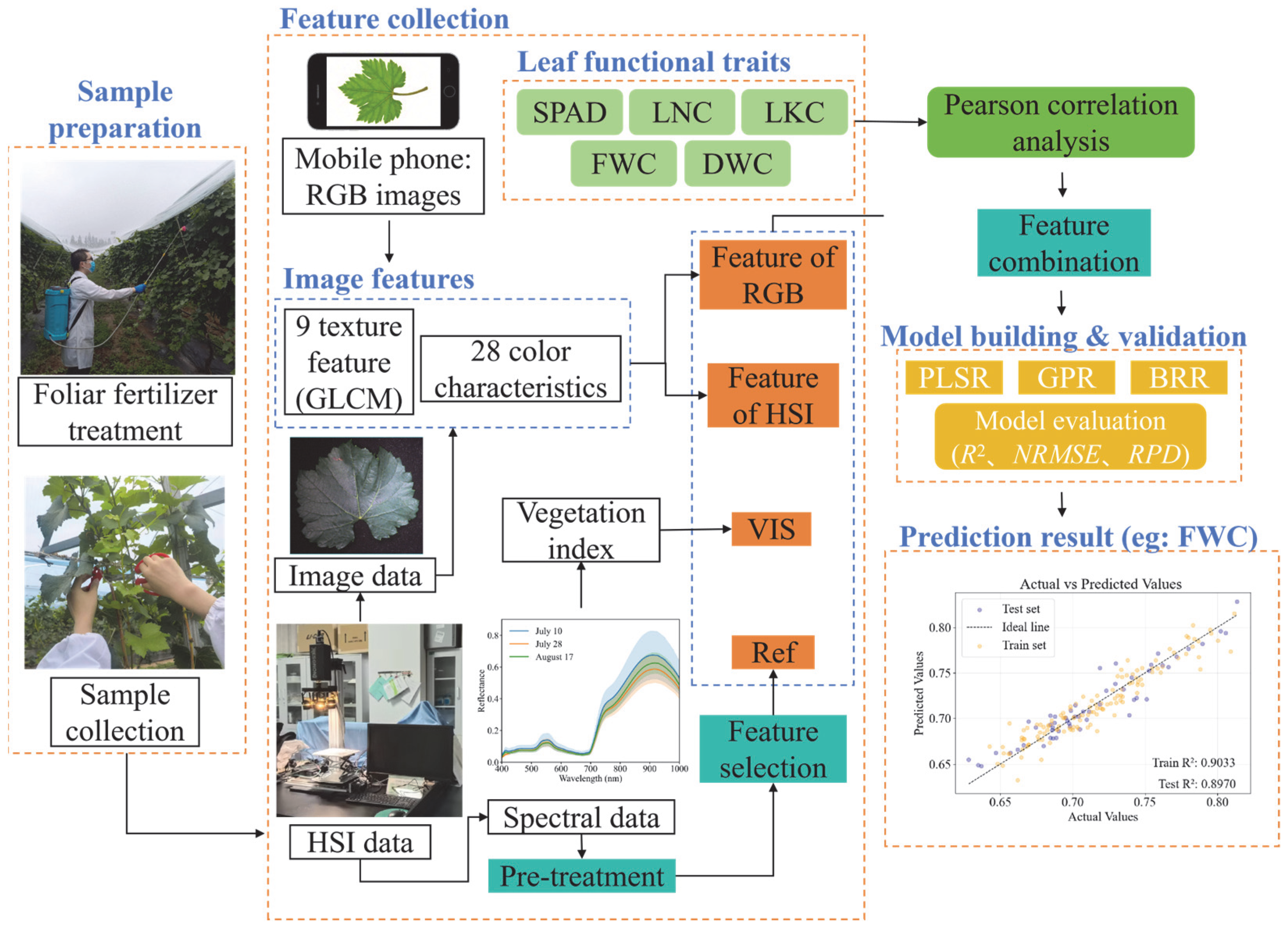
Figure 1. Sample preparation, feature acquisition, and data analysis workflow in this study. Regression algorithms employed include partial least-squares regression (PLSR), Gaussian process regression (GPR), and Bayesian ridge regression (BRR). Leaf functional traits include chlorophyll, expressed as soil and plant analysis development (SPAD); leaf nitrogen content (LNC); leaf potassium content (LKC); fresh weight water content (FWC); and dry weight water content (DWC). Curves show the mean reflectance on three measurement dates (10 July, 28 July, and 17 August). The shaded areas around each curve represent the standard deviation (±1 SD) of the spectral measurements for that date, indicating data variability.
Agronomy 16 00029 g001
Figure 2. Texture features of grape leaves. MEA: mean; VAR: variance; HOM: homogeneity; CON: contrast; DIS: dissimilarity; ENT: entropy; ASM: angular second moment; COR: correlation; and ACOR: autocorrelation.
Agronomy 16 00029 g002
Figure 3. Leaf functional traits under different fertilizer treatments and growth stages: (a) chlorophyll, expressed as soil and plant analysis development (SPAD); (b) leaf nitrogen content (LNC); (c) leaf potassium content (LKC); (d) fresh weight water content (FWC); and (e) dry weight water content (DWC). CH4N2O: urea solution; K2SO4: potassium sulfate solution; KH2PO4: potassium dihydrogen phosphate solution; Mixed: nitrogen–phosphorus–potassium mixed solution. Color symbols: Boxes in red, gray, and blue represent data collected on 10 July, 28 July, and 17 August, respectively.
Agronomy 16 00029 g003
Figure 4. Reflectance of all grape leaf samples. Curves show the mean reflectance on three measurement dates (10 July, 28 July, and 17 August). The shaded areas around each curve represent the standard deviation (±1 SD) of the spectral measurements for that date, indicating data variability.
Agronomy 16 00029 g004
Figure 5. Evaluation metrics for the prediction of grape leaf functional traits using partial least-squares regression (PLSR), Gaussian process regression (GPR), and Bayesian ridge regression (BRR) models under different preprocessing methods. (a) PLSR evaluation metrics; (b) GPR evaluation metrics; and (c) BRR evaluation metrics.
Agronomy 16 00029 g005
Figure 6. Original spectra and feature selection results based on the competitive adaptive reweighted sampling (CARS), least absolute shrinkage and selection operator (LASSO), and recursive feature elimination (RFE) algorithms. Original spectra compared with the (a) chlorophyll soil and plant analysis development (SPAD)-sensitive spectral band; (b) leaf nitrogen content (LNC)-sensitive spectral band; (c) leaf potassium content (LKC)-sensitive spectral band; (d) fresh weight water content (FWC)-sensitive spectral band; and (e) dry weight water content (DWC)-sensitive spectral band. The number of screened features is shown in parentheses.
Agronomy 16 00029 g006
Figure 7. Evaluation metrics for the prediction of grapevine leaf functional traits using partial least-squares regression (PLSR), Gaussian process regression (GPR), and Bayesian ridge regression (BRR) models with different feature selection methods. (a) PLSR evaluation metrics. (b) GPR evaluation metrics. (c) BRR evaluation metrics.
Agronomy 16 00029 g007
Figure 8. Pearson correlation coefficients between the color and texture characteristics of vegetation indices, hyperspectral images, and RGB images with leaf functional traits. Correlation coefficient maps depict correlations between (a) 33 vegetation indices and leaf functional traits; (b) 45 hyperspectral image texture features and leaf functional traits; (c) 28 hyperspectral image color features and leaf functional traits; (d) 9 RGB image texture features and leaf functional traits; and (e) 28 RGB image color features and leaf functional traits. VIS: vegetation index; HSI-Tex: texture features of hyperspectral images; HSI-Col: color characteristics of hyperspectral images; RGB-Tex: texture features of RGB images; and RGB-Col: color characteristics of RGB images. In the texture characteristics of hyperspectral images, “_wavelength” indicates an image extracted from that wavelength. The color gradient in each matrix represents the strength and direction of the Pearson correlation coefficient (r), with yellow indicating strong negative correlations and blue indicating strong positive correlations.
Agronomy 16 00029 g008
Figure 9. RGB images of leaves with different SPAD values. (a) SPAD = 30.44; (b) SPAD = 40.7; and (c) SPAD = 50.08. SPAD: soil and plant analysis development, indicating chlorophyll content.
Agronomy 16 00029 g009
Figure 10. Evaluation metrics for the prediction of grapevine leaf functional traits using partial least-squares regression (PLSR), Gaussian process regression (GPR), and Bayesian ridge regression (BRR) modeling under different feature combination methods. (a) PLSR evaluation metrics. (b) GPR evaluation metrics. (c) BRR evaluation metrics.
Agronomy 16 00029 g010
Figure 11. Performance improvements of optimal preprocessing, feature selection, and feature fusion methods compared with the raw spectral model. (a) R2 increase rate for the partial least-squares regression (PLSR) model; (b) NRMSE increase rate for the PLSR model; (c) RPD increase rate for the PLSR model; (d) R2 increase rate for the Gaussian process regression (GPR) model; (e) NRMSE increase rate for the GPR model; (f) RPD increase rate for the GPR model; (g) R2 increase rate for the Bayesian ridge regression (BRR) model; (h) NRMSE increase rate for the BRR model; and (i) RPD increase rate for the BRR model.
Agronomy 16 00029 g011
Table 1. Feature description.
AcronymFeature TypeFeature Number
RefSpectral reflectance462
VISVegetation indices33
HSI_CTColor and texture features of hyperspectral images73
RGB_CTColor and texture features of RGB images37
Table 2. Optimal preprocessing and feature wavelength selection for leaf traits.
Leaf TraitsPretreatmentsPreprocessing Results (R2)Feature SelectionFeature Selection Results (R2)
SPADSG-PLSR0.8572CARS-PLSR0.8676
LNCMSC-PLSR0.6700CARS-PLSR0.7132
LKCSNV-PLSR0.7127CARS-BRR0.7358
FWCMSC-PLSR0.8611CARS-BRR0.8803
DWCMA-PLSR0.8819LASSO-PLSR0.8724
Note: “Pretreatments-Model” indicates the use of this preprocessing step and model. “Feature selection-Model” indicates that after using the optimal preprocessing, the Feature selection and Model are combined.
Table 3. Number of correlations between different features and leaf functional traits.
Leaf TraitsVISHSI-TexHSI-ColRGB-TexRGB-Col
SPAD333521723
LNC1526474
LKC2873718
FWC26364723
DWC26374722
Disclaimer/Publisher’s Note: The statements, opinions and data contained in all publications are solely those of the individual author(s) and contributor(s) and not of MDPI and/or the editor(s). MDPI and/or the editor(s) disclaim responsibility for any injury to people or property resulting from any ideas, methods, instructions or products referred to in the content.