Abstract
Soil secondary salinization is a major limiting factor of sustainable agricultural production in arid and semi-arid irrigation zones, yet predictive tools for regional water–salt dynamics remain limited. The Yichang Irrigation District, located within the Hetao Irrigation Area, has experienced persistent salinity challenges due to shallow groundwater tables and intensive irrigation. In this study, we aimed to simulate long-term soil water–salt dynamics in the Yichang Irrigation District and evaluate the effectiveness of different engineering and management scenarios using the SaltMod model. Field monitoring of soil salinity and groundwater levels during summer and fall (2022–2024) was used to calibrate and validate SaltMod parameters, ensuring accurate reproduction of seasonal soil salinity fluctuations. Based on the calibrated model, ten-year scenario simulations were conducted to assess the effects of changes in soil texture, irrigation water quantity, water quality, rainfall, and groundwater table depth on root-zone salinity. Our results show that under baseline management, soil salinity is projected to decline by 5% over the next decade. Increasing fall autumn leaching irrigation further reduces salinity by 5–10% while conserving 50–300 m3·ha−1 of water. Sensitivity analysis indicated groundwater depth and irrigation water salinity as key drivers. Among the engineering strategies, drainage system improvement and groundwater regulation achieved the highest salinity reduction (15–20%), while irrigation regime optimization provided moderate benefits (~10%). This study offers a quantitative basis for integrated water–salt management in the Hetao Irrigation District and similar regions.
1. Introduction
Soil secondary salinization is a common problem in arid and semi-arid irrigation areas globally, which seriously constrains agricultural yield, ecological stability, and sustainable regional development [1]. Taking the Hetao Irrigation Area in northwest China as an example, the average annual precipitation is only 150–200 mm, while potential evaporation reaches 2000–3000 mm. This large evaporation–precipitation gap causes rapid surface moisture loss, leading to salt accumulation in the root zone and shallow soil, with continuous upward migration through capillary action, resulting in worsening soil salinization [2].
Under long-term diffuse irrigation, irrigation water brings large amounts of soluble salts to the root zone. Simultaneously, lagging or imperfect drainage systems hinder the timely discharge of salt, causing chronic salt accumulation over multiple years. This process reduces soil biological activity, decreases crop yields, and may even lead to land abandonment [3]. Sustained root-zone salinity of 1.5–2.0 g·kg−1 in the Hetao basin is typically associated with 5–12% maize yield losses and a 5–10% decline in leaf area index, underscoring the agronomic relevance of seasonal desalination.
In the Yichang Irrigation Area, a key agricultural zone within the Hetao Irrigation District, the terrain is flat, with loamy clay as the predominant soil texture. Groundwater depth is consistently between 1.0 and 2.0 m, with mineralization levels of 3–6 g·L−1. In recent years, Huanghuang-induced irrigation has continued to meet the water demand for crop growth, but a serious imbalance exists between the irrigation water volume and evaporation demand in spring and summer, with surface recharge far exceeding evaporation demand [4]. However, surface recharge also exceeds drainage capacity, and the drainage ditches are inefficient, especially during dry periods, resulting in surface soil salinity (0–20 cm) peaking at 1.8 g·kg−1 after summer irrigation. Salinity drops to only 1.2 g·kg−1 following fall drenching, but cumulative salt leaching remains insufficient, and the area of high-salinity patches in the surface soil expands year by year. Salinization is even more severe in downstream low-lying areas, where salt content in some locations exceeds 3.0 g·kg−1 [5]. This cyclical “accumulation–drenching accumulation” process has exacerbated salinization, posing serious challenges to food security and soil quality [6].
Currently, several engineering problems hinder effective irrigation and drainage management in the Yichang Irrigation Area: (1) a lagging drainage system: the sparse distribution of agricultural canals and poor maintenance make it difficult to remove excess water, leading to persistently high groundwater levels [7]; (2) an inefficient irrigation system: the diffuse irrigation mode lacks precision scheduling, with mismatches between irrigation quotas and crop water demands, and insufficient attention to fall autumn leaching irrigation for salt leaching [8]; (3) deteriorating water quality: increased pressure on basin water use has raised the salinity of incoming Yellow River water, contributing further to salt accumulation [9]; (4) high engineering and management costs: investments required for efficient drainage are high, and limited management and maintenance funding make it difficult to achieve sustainable benefits across the entire area [10]. Achieving optimal irrigation and drainage support and precise scheduling have become key challenges for controlling salinization and ensuring the sustainable development of the Yichang Irrigation Area.
Additionally, the spatial and temporal variability in soil salinity and its driving mechanisms have not been deeply and systematically understood. The salinization process is influenced by multiple factors: soil texture determines the efficiency of seepage and capillary rise; groundwater depth affects the degree of surface salt accumulation; irrigation water quantity and quality directly influence salt input; and climatic rainfall provides natural leaching or concentration effects. Existing studies have mostly focused on single-factor effects or small-scale experiments and lack numerical predictions for long-term, multi-scenario conditions under the combined influence of multiple factors [11]. In semi-arid plains, root-zone salinity is primarily modulated by the groundwater table position and salinity, soil hydraulic properties controlling capillary rise and leaching, and seasonal water inputs from rainfall and irrigation.
This is reflected in the following gaps: (1) incomplete understanding of soil texture and salt migration: under different soil conditions, water flow paths and salt transport rates vary significantly, but quantitative coupling analyses are lacking; (2) unclear groundwater–soil interactions: the feedback between groundwater-level dynamics and surface salt concentration is complex, and long-term trend predictions are needed to support management; (3) unclear irrigation–rainfall interactions: the combined leaching and concentration effects of irrigation and rainfall require simultaneous consideration, especially as salt accumulation trends differ between dry and wet years; (4) limited assessment of combined engineering measures: the cumulative effects of drainage, irrigation, and groundwater regulation have not been systematically evaluated, making it difficult to design optimal management strategies under resource constraints.
Therefore, an urgent need exists for a numerical model capable of addressing long-term, multi-factor, and multi-scenario predictions of salinity dynamics, identifying key control factors through sensitivity analysis and providing a scientific basis for engineering measures.
The SaltMod model is based on the principle of empirical water–salt balance at seasonal scales [12]. It divides the soil–groundwater system into several reservoirs (surface water layer, root zone, transition layer, and deep aquifer). It sequentially calculates the water balance of rainfall, irrigation, evapotranspiration, capillary recharge, seepage, and drainage. Salt balance is modeled within the same framework, simulating the salt concentration in each reservoir over time [13]. The model’s data requirements are relatively simple, requiring only seasonal rainfall, irrigation quota and salinity, potential evapotranspiration, soil layer thickness and water-holding capacity, groundwater depth and salinity, drainage coefficient, and drenching efficiency. This enables assessment of salinization trends and drainage needs over multi-year scales [14].
Internationally, SaltMod has been validated and applied in the Nile Delta, the middle Ganges, and arid regions of Europe and the United States. However, its application at the branch-canal scale in China’s Hetao Irrigation District remains rare, with a lack of systematic calibration and validation using field monitoring data. Table 1 summarizes the Saltmod model’s research cases across different regions.

Table 1.
Representative applications of the SaltMod model in different regions.
SaltMod has mostly been applied at the irrigation district scale to predict future salinity trends, revealing a slight decrease in salinity under current management, but with limited regulation potential [17]. The model has also been used to assess water salinity dynamics under different irrigation and drainage management scenarios, demonstrating that increasing drenching irrigation and lowering irrigation conductivity considerably help control salinization [22]. Other studies have analyzed soil salinity evolution and key drivers in the Hetao Irrigation Area using principal component and stepwise regression analyses but have not conducted predictive assessments for future multi-scenario conditions or engineering measures [23]. In summary, while researchers have gained a preliminary understanding of salinity mechanisms and management options, gaps remain in integrating recent observations, conducting long-term simulations, and assessing engineering solutions at the branch-canal scale.
Alternative tools include HYDRUS (rich process detail and short-term infiltration–solute transport at plot scale), SWAP coupled with crop models (soil–water–crop interactions at field scale), and district-scale water allocation models. Compared with these, SaltMod requires modest data, operates at seasonal resolution, and is well suited to branch-canal management analyses while capturing the accumulation–leaching cycle.
We address this gap by implementing a systematic, branch-canal–scale calibration and validation of SaltMod using a two-year multi-season dataset, followed by scenario experiments that couple irrigation scheduling, drainage enhancement, and groundwater regulation. This design moves beyond prior district-level trend assessments by quantifying the relative contributions of management levers to root-zone salinity dynamics and by producing transferable parameter sets for semi-arid canal command areas.
In response to these engineering and scientific challenges, this study focuses on the Yichang Irrigation Area of the Hetao Irrigation District. Using monitoring data on soil salinity and groundwater depth from summer and fall of 2022 to 2024, the SaltMod model is systematically calibrated and validated to ensure stable simulation of seasonal salt accumulation and leaching processes. Multiple scenarios covering soil texture, irrigation quota, water quality change, rainfall conditions, and groundwater regulation were designed for the next 10 years to quantitatively predict the spatial and temporal evolution of salinity [21]. Based on the simulation results, numerical experiments were carried out to assess the long-term effects of three key engineering measures—construction of drainage ditches, optimization of irrigation systems, and groundwater level control—of salinity management.
This study addresses three focused questions at the branch-canal scale: (i) How accurately can SaltMod reproduce seasonal accumulation–leaching cycles under local hydro-agronomic conditions? (ii) Which factors most strongly control root-zone salinity? (iii) What is the expected ten-year desalination under practical management interventions? Accordingly, our objectives were to (1) calibrate and validate SaltMod against observed soil salinity and groundwater depth; (2) perform one-way and Sobol sensitivity analyses to rank key controls; and (3) evaluate the effectiveness of drainage system improvement, irrigation-regime optimization, and groundwater regulation through forward scenarios.
2. Materials and Methods
2.1. Study Area Description
Yichang Irrigation Area is located in the central part of Hetao Irrigation Area in Inner Mongolia, which is a typical branch irrigation area of Hetao Irrigation Area (longitude, 106°45′–106°55′ E; latitude, 38°50′–39°00′ N) [24]. The data for this study were obtained with support from the Inner Mongolia Autonomous Region Field Scientific Observation and Research Station for Agricultural Water and Soil Environment and Comprehensive Utilization of Saline–Alkali Land in the Hetao Irrigation District in China. The total area of the region is about 50 km2 (Figure 1), and the terrain is extremely flat, with an average elevation of 1100 m above sea level, field slopes of less than 0.1%, and negligible surface runoff [25].

Figure 1.
Schematic diagram of topography, main channel, and sampling point distribution in the study area.
The area has a temperate continental semi-arid climate [26]. Long-term observation data show that the average annual precipitation is approximately 180 mm, with more than 70% falling between June and August. The annual potential evapotranspiration is approximately 2200 mm, indicating that evaporation greatly exceeds precipitation. The soil is predominantly loamy clay, and the topsoil layer (0–20 cm) has a soil bulk density of , a field water-holding capacity of , an effective water-holding capacity of , and a saturated hydraulic conductivity of .
Corn is the main crop in the area, with a growing season from May to September. Its crop water demand can be calculated using the FAO Penman–Monteith equation for daily potential evapotranspiration, as shown in Equation (1):
In the formula, represents the slope of the saturated water vapor pressure curve (kPa°C−1), Rn represents the net radiation value (MJm−2d−1), G represents the surface heat flux (MJm−2d−1), represents the dry and wet constants (kPa°C−1), T represents the average daily air temperature (°C), u2 is the average daily wind speed at a height of 2 m (ms−1), and es and ea are the saturated and actual water vapor pressure (kPa), respectively. Long-term data on groundwater depth show an average groundwater depth of 1.5 m, with a seasonal fluctuation range of 1.0–2.0 m. The groundwater mineralization is 3–6 g L−1.
2.2. Field Data Collection
To calibrate and validate the SaltMod model and provide baseline data for scenario simulations, systematic field observations were conducted in the Yichang Irrigation Area from 2022 to 2024.
- Soil salinity. Sixty sample points were arranged on a 1 km × 1 km grid, covering typical plots in the upper, middle, and lower reaches. At each point, three soil samples from 0 to 20 cm were collected and combined. Electrical conductivity (, dS·m−1) was measured on-site using the 1:5 saturated paste extract method, and soil salinity (, g·kg−1) was calculated from using Equation (2).where 0.64 was obtained from regional laboratory calibration. The mean , standard deviation , , and of the sample points were calculated for each period (July for summer and October for fall).
- Groundwater level and water quality. Ten observation wells were set up within 50 m of the sample points, and the depth of groundwater and salinity were measured regularly. The average value of each well was used as the initial groundwater depth and salinity boundary conditions for the SaltMod model.
- Meteorology and hydrology. Two automatic weather stations provided daily data on rainfall, air temperature, wind speed, humidity, and daily radiation, which were used to calculate seasonal rainfall and potential evapotranspiration ET0. Combined with surface hydrological measurements (channel flow, irrigation infiltration, etc.), field irrigation quotas and drainage capacity were estimated. All observations were quality-controlled and used for parameterization and validation of the SaltMod model. The spatial distribution of monitoring points and the statistical characteristics of key variables are illustrated in Figure 1 and Table 2, respectively. To enhance representativeness for long-term simulation, we combined the observed seasonal means with multi-year station climatology to define baseline rainfall and potential evapotranspiration, and we used measured canal operations to constrain irrigation quotas. Groundwater salinity was characterized by repeated sampling at ten wells, and its interannual variability was propagated through sensitivity analysis. These settings ensure that the calibrated parameters reflect process behavior rather than a single-year anomaly.
Table 2. Statistics of measured soil parameters in the Yichang Irrigation District in summer and fall of 2022–2024.
2.3. Fundamental Principles and Structure of the SaltMod Model
Configuration used in this study: We implemented SaltMod with two seasons (growing and non-growing) and four vertical reservoirs, calibrated a small set of process-governing parameters (soil hydraulic conductivity, leaching efficiency, groundwater discharge coefficient, and layer thicknesses), and prescribed boundary conditions from station climatology and canal operations. The calibrated model outputs seasonal soil water content, salt content, groundwater depth, and drainage volumes, which are then analyzed under management scenarios.
The SaltMod model is an empirical water–salt balance model operating on a seasonal scale. Its core idea treats the soil–water–salt system in irrigation areas as a multilayer system of tandem reservoirs, enabling long-term prediction of regional soil moisture, salinity, and groundwater dynamics by establishing water and salt balance for each reservoir.The schematic diagram of the model workflow framework is shown in Figure 2.
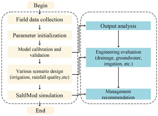
Figure 2.
Model flow framework diagram.
2.3.1. Principle of Water and Salt Mass Conservation
For any horizontal unit (or subarea), SaltMod divides the profile vertically into four reservoirs: the surface water layer, the root-zone soil layer, the transition layer, and the aquifer (submersible aquifer) [27]. Each reservoir adheres to principles of water and salt mass conservation over the simulation period, typically divided into two seasons, “irrigated” and “non-irrigated”.
The water balance equation for the root zone is expressed as Equation (3):
where represents the change in soil water storage in the root zone (mm), P represents rainfall infiltration (mm), I represents irrigation infiltration (mm), Uup represents capillary recharge (lower groundwater rising to the root zone, mm), ETr represents actual evapotranspiration from the root zone (mm), Dr represents the amount of water leaking out of the root zone and into the transition layer (mm), and R represents surface runoff (mm). The corresponding salt balance equation for the root zone is provided by Equation (4):
where represents the change in salt storage in the root zone (kg·ha−1); , , and represent the salt concentration in rainfall, irrigation water, and groundwater, respectively (g L−1); represents the salt concentration in the root-zone leaching water (g L−1); and is the equivalent salt concentration in the soil water of the root zone (converted from the saturated electrical conductivity , g L−1).
2.3.2. Model Structure and Time Domain Division
SaltMod divides the year into 1–4 simulation seasons; in this study, a two-season system of growing and non-growing seasons was adopted. Vertically, the model represents the soil–water–salt system as four sequentially linked reservoirs, each governed by water and salt balance equations. The vertical layers were divided into a surface layer (considering rainfall, infiltration from diffuse irrigation, evaporation, and runoff), a root-zone layer (considering vegetation evapotranspiration, capillary rise, and infiltration), a transition layer (connecting the root zone to the aquifer and buffering upward and downward seepage), and a deeper aquifer (simulating submerged recharge, discharge, and drainage from wells and canals) [28].
The outflow from each reservoir serves as the inflow to the layer below. The groundwater layer can be modeled either with a natural discharge coefficient or a fixed water table boundary to simulate lateral groundwater flow beyond the modeled area [29]. Key model input parameters include seasonal rainfall , potential evapotranspiration , irrigation quota , water quality , crop cover and water consumption, number of growing seasons, land-use ratio, soil thickness, soil water-holding parameters (, , and ), leaching efficiency ( and ), initial soil and groundwater salinity (, ), groundwater depth, and groundwater discharge coefficients. The output parameters were soil water content of each layer in each season (), salt content (), groundwater depth (), drainage volume (), and drainage salt concentration ().
Water–salt coupling was achieved through sequential layer-by-layer mass balance, allowing for simultaneous simulation of water flow and salt transport. Capillary rise was calculated based on the groundwater depth and soil capillary properties [20]. The drainage process was divided into field drainage via agricultural ditches and main canal drainage, which can be established with varying drainage efficiencies. Boundary conditions included an upper boundary driven by rainfall and irrigation, while the lower boundary was set as a fixed water level, specific flux, or no flux conditions [30].
SaltMod enables reliable, large-scale, long-term prediction of soil salinity with low data requirements and efficient seasonal balance calculation, providing quantitative decision support for irrigation and drainage management in irrigated regions.
2.4. Key Modules and Functions of the SaltMod Model
The SaltMod simulation engine consists of three interrelated modules: the soil water balance module, the salt transport module, and the groundwater module, each performing mass conservation calculations at user-defined seasonal intervals [31].
2.4.1. Soil Water Balance Module
For any soil layer i (e.g., surface layer, root-zone layer, or transition layer), this module applied the water balance equation:
where represents the change in soil water storage in layer i (mm), is rainfall infiltration (mm), is irrigation infiltration (mm), represents lower layer capillary recharge (mm), represents actual evapotranspiration from the layer (mm), and is water leakage to the lower layer (mm). Rainfall and irrigation infiltration are calculated by subtracting surface runoff from effective rainfall and irrigation quotas. Actual is calculated by multiplying the FAO-PM potential by the crop coefficient :
Capillary rise is parameterized using an empirical function based on groundwater depth and soil water-holding properties. Leakage is determined by the soil’s saturated hydraulic conductivity and saturated water content.
2.4.2. Salt Transport Module
Based on the water balance, the model establishes salt conservation equations for each soil layer i:
where represents the change in salt storage in layer i (kg·ha−1); , , and represent the salt concentration in rainfall, irrigation water, and groundwater, respectively (g L−1); is the salt concentration in drainage (leaching) water (g L−1); and is the equivalent salt concentration in soil water, calculated from saturated electrical conductivity , g L−1. The leachate salt concentration is coupled with the in-layer salt concentration via the leaching efficiency :
All salts in water lost through evapotranspiration are assumed to remain in the soil, resulting in elevated residual salt concentrations that are not directly discharged.
2.4.3. Groundwater Module
The groundwater module simulated the water and salt exchange between the deepest aquifer, the overlying transition layer, and the external drainage system:
where and represent leakage infiltration and capillary rise from the transition layer, respectively; represents artificial drainage (ditches, pipes, or pumping); represents recharge (channel seepage, recharge); and is the salt concentration of the drainage outflow (g L−1). The rise and fall of the groundwater table, in turn, affect capillary rise , thus closing the soil–groundwater–salt cycle. By iteratively calculating Equations (5)–(9) layer by layer over two simulation seasons, SaltMod simulates coupled water and salt dynamics between soil layers at different depths and groundwater, enabling long-term, large-scale salinity evolution prediction and comparative scenario analysis.
2.5. Parameter Setting and Configuration Under Local Conditions
Based on findings in field observations and the literature, the following key parameters were locally calibrated in this study: (1) soil thickness and water-holding parameters: based on soil drilling results, the root-zone thickness was set to 0–0.30 m, and the transition layer thickness was set to 0.30–2.00 m. The field water-holding capacity and effective water-holding capacity were set as the average values from sample points in the study area [32]. (2) Saturated hydraulic conductivity: the saturated hydraulic conductivity of each layer was determined using double-ring infiltration experiments and corrected to the simulated single-layer values from the root zone and transition layer [33]. (3) Drenching efficiency: root zone and transition layer washing efficiency ( and ) were set at 0.65 and 0.45 by inversion of the net salt change in summer and fall of 2022–2024, respectively [34]. (4) Groundwater discharge coefficient: the seasonal drainage coefficient of the aquifer was determined by inversion, using the density of drainage ditches and measured drainage flow .
For the initial and boundary conditions, the measured soil salinity and groundwater depth before the summer of 2022 were used as the initial values to ensure dynamic consistency for the first simulation season. The upper boundary conditions included seasonal rainfall, irrigation volume, and water quality concentration. Crop coefficients were categorized into early stage (0.7), peak stage (1.15), and late stage (0.8) according to the growth stages of typical maize varieties in the region. For the lower boundary conditions, the aquifer was set as a free water level boundary, allowing groundwater depth to update dynamically during simulation; artificial drainage flux was linked to the deep drainage term based on the ditch drainage efficiency model.
To identify the most critical uncertain parameters, we combined one-factor sensitivity analysis and Sobol global sensitivity analysis. In the one-factor analysis, each parameter was varied by ±20% from its baseline values to assess its impact on end-of-year root-zone salinity and groundwater depth. In the Sobol analysis, key hydraulic and management parameters, such as hydraulic conductivity, leaching efficiency, and drainage coefficient, were used to calculate first-order and total effects indices, quantifying their relative importance under multifactor interactions. The sensitivity results informed the selection of key parameters for subsequent model calibration and scenario design. The workflow—field-based calibration, factor screening, and management scenario testing—is generic and can be ported to other semi-arid canal command areas where seasonal irrigation governs the accumulation–leaching cycle. For reporting uncertainty, we propagated parameter ranges (±20% about calibrated values) through 500 Latin hypercube samples to derive 95% confidence intervals for simulated end-of-year root-zone salinity.
Initial and boundary conditions for reproducibility: Initial root-zone salinity at t0 (summer 2022) was set to the measured 0–20 cm mean within each of the upstream, midstream, and downstream subareas, and assigned uniformly within each subarea. Groundwater depth was initialized from the ten-well network averages. Upper boundary forcings used seasonal rainfall, potential evapotranspiration, and canal-recorded irrigation quotas; groundwater salinity was initialized from repeated well sampling.
2.6. Model Calibration and Validation Methods
The observed values of soil salinity and groundwater depth (a total of 60 time data points) from the summer and fall periods of 2022, covering locations in the upper, middle, and lower reaches, were selected for model calibration. The residual sum of squares between the simulated output and the measured values was used as the evaluation index, applying the objective function minimization method. To test the model’s extrapolation capability, an independent set of observations (60 sample points) from the summer and fall of 2024, which were not used in the parameter optimization process, was employed for validation.
Root mean square error (RMSE), Nash–Sutcliffe efficiency (NSE), and the coefficient of determination (R2) were chosen as model evaluation metrics, as defined by the following equations:
where and are the observed and simulated values of the i-th time, respectively; is the mean of the observed values; and N is the total number of samples. Generally, lower RMSE values and NSE and R2 values closer to 1 indicate better model performance. Long-term projections (2025–2034) therefore represent conditional scenarios under observed management baselines and tested perturbations, rather than forecasts of specific year-to-year weather sequences.
We report 95% confidence intervals (CIs) for the evaluation metrics. For R2, we compute the Pearson correlation r between observed and simulated values, transform with Fisher’s z = atanh (r), use , and back-transform the 95% z interval (z ± 1.96·SE) to obtain the CI for r and hence for R2 (=r2). For RMSE and NSE, we apply a non-parametric bootstrap with 2000 resamples of the paired observations; the 2.5th and 97.5th percentiles of the bootstrap distribution define the 95% CI. We report values as estimate [lower–upper].
2.7. Scenario Design for Future Simulations
To evaluate soil water and salt dynamics under different management and climatic conditions, we designed three sets of scenarios on the calibrated SaltMod model. The first set focused on changes in irrigation amount. In the baseline scenario, the average total irrigation volume of 667 mm·a−1 observed from 2022 to 2024 was used. In the decreased irrigation scenario, the irrigation volume was reduced by 20% to approximately 534 mm·a−1 to assess the risk of salt accumulation under water-saving conditions. In the increased scenario, the irrigation volume was raised by 20%, to approximately 800 mm·a−1, to evaluate the impact of enhanced leaching efficiency and changes in the groundwater table on soil desalination.
The second set examined changes in irrigation water quality. In the clear water scenario, irrigation water conductivity was reduced from the baseline of 1.05 dS·m−1 to 0.6 dS·m−1 to analyze the effects of low-salinity water on root-zone salt balance. In contrast, in the high-salt scenario, irrigation water conductivity was increased to 1.5 dS·m−1 to simulate salt accumulation under deteriorating water quality conditions.
The third set of scenarios explored rainfall variation. In the dry scenario, annual rainfall was decreased by 20%, to approximately 144 mm·a−1, to examine the impact of increased dependence on groundwater and irrigation on salinity dynamics. In the wet scenario, annual rainfall was increased by 20%, to approximately 222 mm·a−1, to investigate how enhanced rainfall influences root-zone leaching and groundwater level decline.
These six one-way scenarios were analyzed in comparison with the baseline scenario to quantify the effects of irrigation management and climatic factors on soil salinity trends over the next 10 years. The simulation scenarios and boundary conditions for SaltMod are summarized in Table 3.
Table 3.
Simulation scenarios and boundary settings for SaltMod.
2.8. Engineering Management Scenarios
To assess the effects of different engineering measures on salinity control in the simulation, we established three types of engineering management scenarios based on the baseline scenario, with parameterization as follows. The first scenario involves drainage system improvement. In this scenario, the depth of field drainage ditches was increased from 1.5 m to 2.0 m, and the lateral spacing of the ditches was reduced from 100 m to 75 m, increasing the drainage coefficient from 0.02 d−1 to 0.035 d−1. Additionally, an underground seepage pipe network (pipe diameter, 0.1 m; burial depth, 2 m; spacing, 50 m) was installed at the bottom of the transition layer, simulating a 20% increase in the drainage capacity and a corresponding improvement in the aquifer discharge coefficient.
The second scenario focuses on adjusting the frequency and regime of irrigation. For the “additional fall leaching” case, the annual irrigation quota increased by 80 mm (from 667 to 747 mm·a−1). For the “frequency increase” case, the annual quota was kept at 667 mm·a−1 but redistributed across seven events. Under the phased drenching intensification approach, a small additional quota of autumn irrigation was introduced alongside the baseline spring and summer irrigation, specifically aimed at removing residual salts from the root zone. In the irrigation cycle optimization approach, the interval between individual irrigations was shortened from an average of 20 d to 15 d, increasing the total number of irrigations from five to seven times per year. This ensures that the soil water content was maintained at 70% to 80% of the field water-holding capacity, achieving a balance between salt control and water conservation.
The third scenario addresses artificial groundwater regulation. In this case, pumping wells were installed in downstream low-lying areas, with three groups of deep wells (well depth, 3 m; pumping capacity, 10 m3·h−1), raising the average groundwater depth from 1.5 m to 1.8 m and reducing the intensity of capillary recharge. Additionally, during peak drainage seasons, combined with agricultural and industrial water reuse, quantitative recharge was applied to the transition layer to simulate a “pumping–return” cycle in the aquifer. This process allows for the gradual dilution of groundwater salinity through the optimization of return irrigation water quality [35]. Figure 3 illustrates the seasonal variation trends of soil salinity and groundwater depth in the Yichang Irrigation Area from 2022 to 2024.
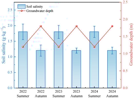
Figure 3.
Seasonal variation in soil salinity (mean ± SD) and groundwater depth (2022–2024).
By parameterizing the three engineering solutions described above and applying them to the SaltMod model, we quantified the emission reduction effect of each measure on soil salinity dynamics over the next 10 years, providing decision support for prioritizing and combining engineering measures under limited resource conditions in the irrigation area.
3. Results
3.1. Calibration and Validation of the SaltMod Model
To evaluate the applicability of the SaltMod model in the Yichang Irrigation Area, we used observation data from the summer and fall of 2022 to 2023 for parameter calibration and data from the summer and fall of 2024 for independent validation. The calibration process employed a genetic algorithm to minimize the residual sum of squares between soil salinity and groundwater depth as the objective function.
As shown in Table 4, the SaltMod model demonstrates strong agreement between simulated and observed values for both soil salinity and groundwater depth. During the calibration period, the RMSE for soil salinity was 0.12 g·kg−1, with an NSE of 0.87 and a coefficient of determination (R2) of 0.90. The relative error was controlled within 6.7%, indicating excellent consistency between simulations and measurements. For groundwater depth, the model successfully reproduced seasonal fluctuation patterns, achieving RMSE = 0.20 m, NSE = 0.83, and R2 = 0.88. The relative error remained within 11.1%, reflecting reliable simulation accuracy.
Table 4.
SaltMod model calibration and validation metrics.
In the validation period, the model maintained robust predictive performance. Simulated soil salinity remained well aligned with observations, despite slight data dispersion, yielding RMSE = 0.15 g·kg−1, NSE = 0.81, and R2 = 0.85. Similarly, the groundwater depth simulations effectively captured the seasonal decline following autumn drainage, with minor deviations in peak and valley amplitudes. Groundwater depth metrics reached RMSE = 0.25 m, NSE = 0.78, and R2 = 0.82, with a relative error of 13.0%. These results confirm the model’s ability to simulate key soil–water–salt dynamics in the Yichang Irrigation Area with acceptable accuracy.
Although the model’s extrapolation performance during the validation period was slightly lower than during calibration, its overall predictive capability remained strong. The model reliably captured both the salt accumulation and leaching cycles, as well as seasonal variations in groundwater depth.
3.2. Observed Spatiotemporal Characteristics of Soil Salinity
Using measured data from two growing seasons in 2022–2023, this study revealed significant spatial and temporal variability in soil salinity across the Yichang Irrigation Area. Spatially, in the upstream zone (sample points 1–10), the average root-zone salinity (0–20 cm) was 1.62 ± 0.48 g·kg−1 in summer, which decreased to 1.05 ± 0.42 g·kg−1 in fall after washing owing to higher topography and relatively favorable drainage conditions. In the middle reaches, average salinity was 1.85 ± 0.60 g·kg−1 in summer, decreasing to 1.25 ± 0.55 g·kg−1 in autumn. In the low-lying downstream area (sample points 21–30), the average root-zone salinity was 1.62 ± 0.48 g·kg−1 in summer, decreasing to 1.05 ± 0.42 g·kg−1 in autumn after drenching. Within this area, peak salinity levels reached as high as 2.10 ± 0.70 g·kg−1 in summer due to the shallow groundwater table before dropping to 1.40 ± 0.65 g·kg−1 in fall. In Figure 3, error bars represent ±1 standard deviation across the 60 sampling points sampled each season, summarizing spatial variability within the branch-canal command area.
In the vertical distribution, the surface root zone (0–20 cm) was most significantly affected by evapotranspiration concentration and irrigation water washing, showing the highest salinity level, averaging 1.80 ± 0.55 g·kg−1 in summer. The middle layer (20–50 cm) exhibited slightly lower salinity due to the accumulation of downward seepage, with salinity levels of 1.42 ± 0.50 g·kg−1 in summer and 1.05 ± 0.46 g·kg−1 in fall, respectively. Overall, the salt concentration showed a gradient distribution from the midstream to the upstream and downstream areas, with the greatest fluctuation occurring in the surface layer, reflecting the differences in how topography and drainage conditions influence salinization.
In the time dimension, soil salinity exhibited a typical “accumulation–drenching” cycle. During the period of high temperatures and strong evaporation from May to September each year, continuous irrigation combined with intense transpiration led to gradual accumulated surface salt accumulation, peaking in August at an average of 1.80 g·kg−1. After October, the combined effects of rainfall and fall drenching irrigation significantly reduced surface salinity, with the average dropping to 1.20 g·kg−1. Interannual comparisons showed that the summer peak in 2023 (1.75 g·kg−1) was slightly lower than in 2022 (1.82 g·kg−1), and the fall peak decreased from 1.22 g·kg−1 to 1.17 g·kg−1. This was mainly attributed to an approximately 8% increase in annual rainfall in 2023 and improvements in localized drainage works. Overall, the seasonal cycle remains the dominant pattern of salinity dynamics in the area, while the interannual trend shows a slight decrease due to the combined influence of climatic and engineering interventions. These patterns are consistent with the sensitivity ranking, which points to groundwater depth and irrigation salinity as first-order controls, with soil texture and rainfall exerting secondary effects.
3.3. Predicted Soil Salinity Dynamics Under Different Scenarios
After the successful calibration and validation of the SaltMod model, we simulated the evolution of root-zone soil salinity (0–20 cm) from 2025 to 2034 under the baseline and four alternative scenarios: autumn leaching, groundwater regulation, irrigation regime adjustment, and reduced rainfall (Figure 4).
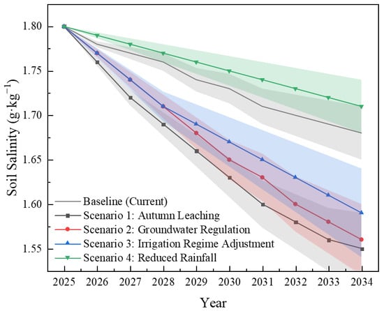
Figure 4.
Simulated soil salinity under management and climate scenarios (median ± 95% CI, 2025–2034). Shaded bands denote the 95% confidence intervals (2.5–97.5th percentiles) obtained from a 500-member Latin-hypercube ensemble with ±20% parameter perturbations.
Under the baseline scenario, which maintained the average management conditions observed during 2022–2024 (irrigation volume of 667 mm·a−1, irrigation water EC = 1.05 dS·m−1, rainfall = 180 mm·a−1, and groundwater depth = 1.5 m), soil salinity gradually decreases from 1.80 to 1.71 g·kg−1 over 10 years—a cumulative reduction of ~5%. The decline was most pronounced during the first five years, after which it stabilized.
In the autumn leaching scenario, additional post-harvest irrigation significantly enhanced salt leaching efficiency. Therefore, soil salinity steadily declined to 1.55 g·kg−1 by 2034, representing a cumulative reduction of approximately 14%—the most effective among all tested interventions.
Under the groundwater regulation scenario, where groundwater levels were artificially lowered to enhance drainage, salinity decreased to 1.60 g·kg−1 by 2034 (~11% reduction), indicating notable benefits for salt removal through deeper percolation.
The irrigation regime adjustment scenario introduced optimized irrigation frequency and timing to improve water-use efficiency. This strategy reduced salinity to approximately 1.66 g·kg−1 (~8% reduction), balancing effective salt control with practical water-saving benefits.
Conversely, the reduced rainfall scenario simulated a 20% decline in annual precipitation, reflecting a potential climate change stressor. This led to a gradual accumulation of soil salinity, reaching 1.75 g·kg−1 by 2034 (~5% increase), highlighting the sensitivity of the root zone to reduced natural leaching.
These results collectively suggest that while salinity shows a mild declining trend under current management, proactive interventions—particularly autumn leaching and groundwater regulation—can markedly enhance soil desalination. In contrast, unfavorable climatic conditions such as reduced rainfall could reverse these gains and exacerbate salt accumulation.
These results indicate that irrigation quantity, water quality, and rainfall changes all had significant effects on the evolution of soil salinity. Among them, irrigation water quality and irrigation quantity adjustment emerged as the most direct and effective means of salinity regulation, while rainfall changes primarily influenced interannual variability. The synergistic effects of drainage and groundwater level control measures will be further evaluated in subsequent engineering scenarios. Across scenarios, the 95% confidence half-width for year-10 salinity was 0.03–0.05 g·kg−1, indicating that the relative ranking of interventions is robust.
3.4. Sensitivity Analysis of the SaltMod Model
To clarify the extent of the influence of different input parameters on soil salinity prediction results, we used a combination of one-way variability analysis and Sobol global sensitivity analysis to evaluate the sensitivity of five types of key parameters: groundwater burial depth, irrigation water conductivity, root-zone saturated hydraulic conductivity, leaching efficiency, and drainage coefficients. The results showed that groundwater depth and irrigation salinity were the most sensitive parameters affecting soil salinity simulation in SaltMod, while soil texture and rainfall exhibited relatively lower sensitivity (Figure 5).
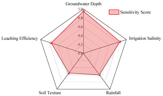
Figure 5.
Sensitivity analysis of the SaltMod parameters.
First, the response of root-zone (0–20 cm) salinity to parameter perturbations was calculated using a one-factor sensitivity test in which each parameter was varied individually within ±20% of its baseline value while keeping other parameters constant. The results showed that groundwater depth and irrigation water conductivity were the most sensitive parameters influencing salinity. When the groundwater depth decreased by 20% (i.e., from 1.5 m to 1.2 m), root-zone salinity increased by about 8% after 10 years. Similarly, when irrigation water conductivity increased by 20% (from 1.05 to 1.26 dS·m−1), salinity rose by nearly 7%. In contrast, changes in root-zone saturated hydraulic conductivity and leaching efficiency had a moderate impact on salinity (3–5% increase or decrease), while the drainage coefficient had the smallest effect (around 2%).
Secondly, Sobol global sensitivity analysis was conducted to quantify both the individual effects and the interactions among the five parameters, by calculating the first-order sensitivity index () and the total effect index (). The results showed that groundwater depth had the highest sensitivity, with Si = 0.42 and STi = 0.53, followed by irrigation water conductivity (Si = 0.30, and STi = 0.40). Leaching efficiency and root-zone saturated hydraulic conductivity showed moderate sensitivity (STi = 0.25 and 0.22, respectively), while the drainage coefficient exhibited the lowest sensitivity (STi < 0.15).
These findings revealed that a shallower groundwater depth intensified capillary rise, leading to continuous recharge of the root zone by saline groundwater. Simultaneously, irrigation water conductivity directly determined the salt input from irrigation, and the combined effect of these two parameters played a dominant role in salt accumulation. Drenching efficiency and saturated hydraulic conductivity influenced the rate of salt infiltration, while the drainage coefficient adjusted the aquifer’s drainage capacity but had a limited direct effect on root-zone salinity due to constraints of the drainage system.
In summary, future applications of the model and the mitigation strategies should focus on groundwater level management and irrigation water quality control to achieve the most significant salinity reduction.
3.5. Impact of Engineering Measures on Soil Salinity
Based on the three types of engineering management programs designed, we numerically simulated root-zone soil salinity (0–20 cm) over the next 10 years (2025–2034), and the results are as follows. Figure 6 illustrates that groundwater regulation and drainage system improvement were the most effective engineering measures for reducing soil salinity, achieving reductions of 0.20 and 0.18 g·kg−1, respectively.
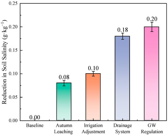
Figure 6.
Reduction in root-zone soil salinity after 10 years for candidate engineering measures (mean ± 95% CI).
Under the drainage system improvement scenario, the depth of field drainage ditches was increased from 1.5 m to 2.0 m, and the ditch spacing was reduced from 100 m to 75 m, which improved the drainage coefficient from 0.02 d−1 to 0.035 d−1. The simulation results showed that after 10 years, soil salinity in the root zone decreased from 1.71 g·kg−1 (baseline) to 1.40 g·kg−1, representing a cumulative reduction of about 18%. When a network of infiltration pipes (0.1 m pipe diameter and 50 m spacing) was further deployed at the bottom of the transition layer, salinity decreased to 1.45 g·kg−1, a reduction of approximately 15%.
Under the irrigation regime optimization scenario, based on the baseline irrigation (five times per year, totaling 667 mm·a−1), two improvements were simulated: adding one additional fall autumn leaching irrigation of 80 mm and increasing irrigation frequency from five to seven times per year. The results showed that additional fall irrigation reduced soil salinity to 1.56 g·kg−1 after 10 years, a reduction of about 9%, while increasing irrigation frequency reduced salinity to 1.60 g·kg−1, a reduction of around 7%. This optimization achieved a balance between water conservation and desalination.
Under the groundwater regulation scenario, the average groundwater depth was raised to 1.8 m by deploying deep wells in the downstream low-lying area (3 m deep wells with a pumping capacity of 10 m3·h−1 × three ports) or through rhythmic recharge combined with industrial and agricultural water reuse to dilute saline water. The pumping scenario reduced soil salinity to 1.48 g·kg−1 after 10 years, a reduction of about 13%, while the combined recharge scenario reduced salinity to 1.50 g·kg−1, approximately a 12% decrease.
Autumn leaching improves desalination at the cost of approximately 80 mm·a−1 of additional water, whereas the frequency increase option preserves the annual quota by redistributing events. Thus, these simulations indicated that drainage system improvement and groundwater regulation were the most effective measures, each achieving 15–20% desalination, while irrigation regime optimization enhanced water-use efficiency but reduced salinity by only about 10%. The synergistic application of multiple engineering measures could provide practical solutions for managing salinized irrigation areas.
4. Discussion
4.1. Mechanisms and Implications of Observed Spatiotemporal Salinity Dynamics
By comparing the measured data with the simulation results of the SaltMod model for 2022–2023, we quantitatively verified the model’s reliability in reproducing the characteristics “summer salt accumulation–autumn flushing” cycle in the Yichang Irrigation Area. The SaltMod simulations faithfully reproduced this seasonal fluctuation and successfully captured the salinity gradient across different soil depths and topographic units. This comparison indicated that the model’s parameterization of key processes—capillary rise, seepage flushing, and drainage—accurately represented the underlying mechanisms of water–salt cycling in the field.
Figure 7 illustrates the spatial distribution of soil salinity across different sampling rows (I–VI) and columns (A–J), revealing significant spatial heterogeneity. Localized salt accumulation was observed in areas such as point III-E.
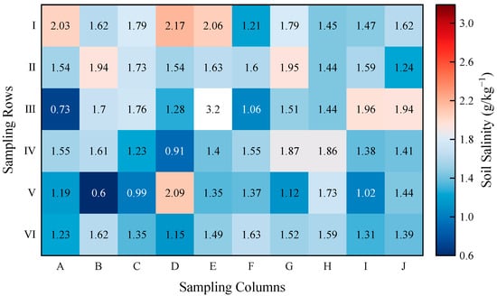
Figure 7.
Spatial distribution of soil salinity.
The region-specific soil salinity patterns were mainly driven by the following factors: first, topographic differences created a clear groundwater depth gradient between upstream (deeper groundwater) and downstream (shallower groundwater) areas. In the upstream, weak capillary rise led to lower salt accumulation, while the downstream area experienced a high-water table and strong capillary rise, resulting in pronounced salinity accumulation. The midstream area, characterized by flat but poorly drained topography, showed the highest peak salinity.
Secondly, irrigation management played a decisive role in the seasonal salt cycle: large-volume irrigation during spring and summer exacerbated salt accumulation, while a single low-volume autumn leaching irrigation was insufficient to fully remove residual salts from the root zone.
Third, while interannual rainfall fluctuations influenced drenching efficiency to some extent, their overall impact on salinity dynamics was weaker compared to the effects of irrigation volume and water quality.
Both the simulation and field observation consistently highlighted that effective water–salt management in semi-arid irrigation areas requires an integrated approach which carefully balances topography, groundwater regulation, and irrigation practices to achieve sustainable salinity regulation and agricultural productivity.
4.2. Reliability and Uncertainty in Model Predictions
Although the reproducibility of the SaltMod model in the Yichang Irrigation Area was improved through systematic calibration and validation in this study, multiple sources of uncertainty remained in the prediction results.
First, soil physical parameters (e.g., saturated hydraulic conductivity, field water-holding capacity) and leaching efficiency, which were obtained from field experiments or inversion, were subject to measurement errors and spatial variability. These uncertainties could lead to biases in simulation results across different grids or years. Second, uncertainties in meteorological and irrigation data (e.g., uneven rainfall distribution, statistical errors in irrigation volume) could also amplify inaccuracies in water–salt balance calculations. In addition, SaltMod assumed homogeneous soil layers and stable boundary conditions, thereby overlooking the sudden impacts of surface runoff, small-scale topographic variations, and extreme climatic events on water and salt transport within the watershed.
The sensitivity analysis indicated that a 20% perturbation in key parameters could result in more than a 10% fluctuation in simulated root-zone salinity. This finding underscored the importance of careful attention to parameters such as groundwater depth and irrigation water conductivity. Structurally, SaltMod adopted a seasonal equilibrium method, which limited its ability to capture short-term pulsations and nonlinear processes, such as transient leaching after heavy rainfalls or changes in capillary rise during extreme droughts. Consequently, its predictive accuracy at interannual and plot scales was constrained. Quantitatively, interval widths from the sampling-based propagation (0.03–0.05 g·kg−1 at year ten) are small relative to intervention effects, supporting the stability of management rankings.
In conclusion, although SaltMod effectively reflected long-term and large-scale salinization trends, it remained limited by parameter uncertainty, data resolution, and structural simplifications. To enhance reliability and accuracy in regional applications, integrating SaltMod with mesoscale or high-resolution models and strengthening field monitoring and data collection are necessary.
4.3. Practical Implications of Scenario Predictions and Management Recommendations
The scenario simulation results demonstrate that various management strategies offer distinct advantages in alleviating salinization but must be tailored to local conditions, including cost, technological maturity, and water resource availability. Based on the simulations and sensitivity analyses, the following practical implications and priority recommendations are proposed:
- Prioritize improved drainage systems. Deepening field drainage ditches and reasonably reducing ditch spacing significantly improve drainage efficiency (with the drainage coefficient increased from 0.02 d−1 to 0.035 d−1 in the model), achieving a 15–20% long-term reduction in soil salinity. This measure involves manageable civil investment, relies on mature construction technology, and is recommended as the primary engineering intervention.
- Implement groundwater-level regulation in parallel. Deploying shallow pumping wells or establishing synchronized recharge systems can raise the average groundwater depth to 1.8 m, thereby reducing capillary rise and achieving approximately 14% salt reduction. This strategy can be combined with drainage system improvements, utilizing the extracted saline groundwater for staged reuse or safe discharge to enhance water resource efficiency.
- Optimize irrigation quotas and frequency. Adding one fall drenching irrigation event (80 mm) and increasing irrigation frequency from five to seven times per year can reduce salinity by 8–10%, with only a modest increase in water consumption. Precise scheduling of irrigation quotas and timing meets both crop water demand and salt leaching requirements. With low technical requirements and minimal management costs, this measure is suitable for rapid adoption.
- Improve irrigation water quality. Where feasible, the preferential use of low-salinity water sources (EC ≤ 0.6 dS·m−1) or the targeted blending of water sources can achieve around 15% salinity reduction over ten years. However, this option is often constrained by water availability and distribution costs and should be pursued as part of a medium- to long-term strategy.
Considering construction costs, effectiveness, and technological readiness, the program should be gradually implemented in the following order: drainage system improvement > groundwater level control > optimization of irrigation system > water quality improvement. Establishing a stable groundwater depth barrier through drainage enhancement and groundwater regulation, combined with precision irrigation and high-quality water sources, will build a “drainage–control–irrigation–quality” synergistic management system to effectively alleviate the risk of salinization in the Yichang Irrigation Area and similar semi-arid regions. Only by adopting such an integrated management approach can salinization risks be mitigated and the sustainable development of agriculture ensured.
4.4. Potential Agricultural Implications of Soil Salinity Dynamics
Based on the simulation results, soil salinity in the root zone (0–20 cm) of the Yichang Irrigation Basin is projected to decrease gradually, by approximately 5% in the next 10 years, under baseline management conditions. However, a reduction in irrigation quantity or deterioration in water quality may lead to more than a 10% increase in salinity. Salinity levels between 1.5 and 2.0 g·kg−1 can induce salt stress in maize, causing a 5–10% decrease in leaf area index and an 8–12% reduction in both stem and leaf biomass and ear kernel yield. The simulation further indicated that adopting low-salinity irrigation water or enhanced drainage could reduce soil salinity to below 1.3 g·kg−1, effectively eliminating salt stress during mid-to-late growth stages and restoring crop yields to non-stressed levels. We did not explicitly couple a crop growth model; thus, yield responses were not simulated. Interpreting salinity effects on yields therefore relies on literature-based response functions, and the quantitative values reported here should be viewed as indicative rather than predictive.
To mitigate the impacts of salinity on crop growth, agronomic management should focus on the following strategies:
Variety selection and planting schedule: salinity-tolerant maize cultivars should be promoted and spring or late sowing should be adopted to avoid peak salinity periods, reducing the risk of salt stress during seedling establishment and nodulation.
Crop rotation and intercropping: maize should be followed with deep-rooted crops (e.g., sunflower, alfalfa) to extract salts from the deeper soil layers, improve soil structure, and encourage the upward movement and subsequent leaching of salts.
Targeted leaching and fertilizer management: an amount of 60–80 mm of water should be applied during autumn leaching, and fertilizer application should be timed to coincide with drenching. Supplementation of potassium and phosphorus should be used to improve salt tolerance, and small nitrogen doses should be provided during drought to improve crop resilience.
Soil improvement and mulching: straw or plastic mulch should be used to reduce evapotranspiration and salt concentration at the surface. In heavily salinized areas, soil amendments such as biochar or gypsum should be applied to improve ion balance, soil aggregation, and water–salt transport efficiency.
By integrating these agronomic practices with the engineering interventions recommended by the model, a synergistic approach to drainage, drenching, and nutrient management can be achieved. This combined strategy will minimize salt stress impacts on crop performance and support the sustainable development of agriculture in the Yichang Irrigation Area.
4.5. Study Limitations and Directions for Future Research
Although this study has successfully reproduced the dynamics of soil water and salinity, as well as the anticipated effects of engineering interventions in the Yichang Irrigation Basin through systematic field observations and model calibration, several limitations remain:
- Limited spatial and temporal coverage: observations were confined to two years and limited to summer and fall, making it difficult to fully capture the impacts of long-term hydrological cycles (e.g., dry and wet years) and extreme climatic events on salinity dynamics.
- Simplified modeling assumptions: SaltMod assumes a homogeneous and level soil and groundwater system, overlooking the influence of microtopographic variation, heterogeneous soil properties, and discontinuous drainage pathways on water and salt movement.
- Lack of crop–salt interaction modeling: this model does not directly couple soil salinity dynamics with crop growth processes, limiting its ability to simulate real-time feedback from salt stress on crop physiology or to reflect the role of root development in modifying water and salt transport.
- Insufficient socio-economic and management assessment: this analysis lacks detailed evaluations of the technical and economic feasibility of the proposed engineering measures. Data on local farmer acceptance, operation and maintenance costs, and long-term sustainability are also lacking. The summary of engineering measures and expected benefits is shown in Table 5.
Table 5. Summary of engineering measures and expected benefits.
To address these shortcomings, future research should extend the observation period and continuously monitor changes in soil salinity, groundwater depth, and crop yields across multiple years, including periods of extreme drought and flooding. This would enhance the model’s capacity to respond to interannual fluctuations and sudden climatic changes. Integrating SaltMod with coupled models that simulate soil–water–crop interactions, such as SWAP-EPIC, would enable the joint simulation of salt stress and crop yield within a unified framework, improving the precision of agronomic management assessments. Incorporating high-resolution spatial data, including topographic elevation and remotely sensed soil salinity inversion, can support the development of refined grid-based models that capture the influence of microtopographic variability on salinity dynamics. Additionally, integrating economic and social analyses, such as cost–benefit evaluations and models of farmer decision-making, would provide critical insight into the economic feasibility, adoption likelihood, and long-term sustainability of various engineering and management strategies. Advancing research in these directions will strengthen both the theoretical and practical foundations of water and salinity management in semi-arid irrigation regions, supporting more precise, adaptive, and sustainable agricultural development.
5. Conclusions
Based on measured data from the summer and fall of 2022–2024, we systematically evaluated and applied the SaltMod model to calibrate, validate, and simulate soil water and salt dynamics in the Yichang Irrigation Area of Hetao Irrigation District, Inner Mongolia. The main conclusions are as follows:
- SaltMod model reliabilityAfter parameter optimization and independent validation, SaltMod accurately reproduces the seasonal accumulation and leaching processes of soil salts in the root zone (0–20 cm), as well as the cyclic fluctuations in groundwater depth. The RMSEs for the calibration and validation periods were below 0.15 g·kg−1 and 0.25 m, respectively, and the NSEs exceeded 0.78, indicating good model performance for long-term regional predictions.
- Identification of key control factorsSensitivity analysis showed that groundwater depth and irrigation water conductivity are the two most influential factors affecting salt dynamics in the root zone, followed by soil leaching efficiency and saturated hydraulic conductivity. The influence of the drainage coefficient was relatively weak. Future water and salt management should prioritize water quality control and groundwater regulation.
- Engineering management program preferencesSimulation results showed that improved drainage (deeper furrows, seepage pipe networks) and artificial water table regulation (deep well pumping or recharge) can achieve a 15–20% reduction in root-zone salinity. Optimized irrigation regimes (additional fall irrigation or increased frequency) can reduce salinity by 7–10%, while using low-salinity irrigation water (EC ≤ 0.6 dS·m−1) can further reduce salinity by about 15%.
- Practical implications and recommendations for sustainable managementThis study provides an engineering roadmap based on quantitative modeling for the Yichang Irrigation Area and similar semi-arid regions. Because inputs are limited to routinely observed variables and canal operation records, the approach is readily transferable to branch-canal systems in other semi-arid regions. It recommends improved drainage and groundwater regulation to build a dual “drainage–control” barrier, supported by precision irrigation and high-quality water sources to enhance “irrigation–quality” synergy. Our results validate the applicability of SaltMod for long-term water and salt prediction at the branch-canal scale and provide a scientific basis for decision-making on integrated water and salt management in irrigation districts, supporting sustainable agricultural development and comprehensive saline–alkali land management. By relying on routinely observed variables and canal operation records, the workflow provides decision support for sustainable irrigation and drainage at branch-canal scale and is readily transferable to other semi-arid systems.
Author Contributions
All authors contributed to the conception and design of the study. Y.S.: conceptualization, data analysis, and manuscript drafting and revision. L.W.: conceptualization and manuscript review and critical revision for important intellectual content. S.Y.: conceptualization, experimental design, sample collection, and chemical analysis. Z.Q.: manuscript review and critical revision for important intellectual content. D.Z.: conceptualization, experimental design, sample collection, and chemical analysis. All authors have read and agreed to the published version of the manuscript.
Funding
This research was jointly supported by the National Natural Science Foundation of China (No. U24A20179), the project for Construction of Leading Talents and Innovative Teams in Science and Technology in the Inner Mongolia Autonomous Region (BR22-13-12), the “Talents Enriching Inner Mongolia” Project of the Inner Mongolia Autonomous Region of China (the team for technological innovation in solid waste resource utilization and salt–alkali land ecological restoration in the Yellow River Irrigation Area) and State Key Laboratory of Water Engineering Ecology and Environment in Arid Area, Inner Mongolia Agricultural University (SQ2024SKL080).
Institutional Review Board Statement
This study did not involve humans or animals.
Data Availability Statement
The original contributions presented in this study are included in this article. Further inquiries can be directed to the corresponding author(s). Processed datasets, SaltMod parameter files, and scenario scripts are available from the corresponding author upon reasonable request.
Acknowledgments
We would like to thank the editors and the anonymous reviewers for their work, helpful suggestions, and comments.
Conflicts of Interest
The authors declare that they have no conflicts of interest.
References
- Stavi, I.; Thevs, N.; Priori, S. Soil Salinity and Sodicity in Drylands: A Review of Causes, Effects, Monitoring, and Restoration Measures. Front. Environ. Sci. 2021, 9, 16. [Google Scholar] [CrossRef]
- Han, L.; Liu, D.; Cheng, G.; Zhang, G.; Wang, L. Spatial distribution and genesis of salt on the saline playa at Qehan Lake, Inner Mongolia, China. CATENA 2019, 177, 22–30. [Google Scholar] [CrossRef]
- Qi, Z.; Feng, H.; Zhao, Y.; Zhang, T.; Yang, A.; Zhang, Z. Spatial distribution and simulation of soil moisture and salinity under mulched drip irrigation combined with tillage in an arid saline irrigation district, northwest China. Agric. Water Manag. 2018, 201, 219–231. [Google Scholar] [CrossRef]
- Ren, D.; Wei, B.; Xu, X.; Engel, B.; Li, G.; Huang, Q.; Xiong, Y.; Huang, G. Analyzing spatiotemporal characteristics of soil salinity in arid irrigated agro-ecosystems using integrated approaches. Geoderma 2019, 356, 113935. [Google Scholar] [CrossRef]
- Zhang, Y.; Yang, P.; Liu, X.; Adeloye, A.J. Simulation and optimization coupling model for soil salinization and waterlogging control in the Urad irrigation area, North China. J. Hydrol. 2022, 607, 127408. [Google Scholar] [CrossRef]
- Slama, F.; Gargouri-Ellouze, E.; Bouhlila, R. Impact of rainfall structure and climate change on soil and groundwater salinization. Clim. Change 2020, 163, 395–413. [Google Scholar] [CrossRef]
- Lv, Z.; Ma, L.; Zhang, H.; Zhao, Y.; Zhang, Q. Environmental and hydrological synergies shaping phytoplankton diversity in the Hetao irrigation district. Environ. Res. 2024, 263, 120142. [Google Scholar] [CrossRef]
- Zhao, Y.; Miao, Q.; Shi, H.; Li, X.; Yan, J.; Yang, S.; Hou, C.; Yu, C.; Feng, W.; Hao, J. Inversion of soil salinization at the branch canal scale in the Hetao Irrigation District based on improved spectral indices. Agric. Water Manag. 2025, 316, 109608. [Google Scholar] [CrossRef]
- Wichelns, D.; Qadir, M. Achieving sustainable irrigation requires effective management of salts, soil salinity, and shallow groundwater. Agric. Water Manag. 2015, 157, 31–38. [Google Scholar] [CrossRef]
- Li, S.; Li, C.; Yao, D.; Wang, X.; Gao, Y. Bowl effect of irreversible primary salinization driven by geology in Hetao irrigation area, China. Sci. Total Environ. 2024, 920, 170834. [Google Scholar] [CrossRef]
- Sun, G.; Zhu, Y.; Ye, M.; Yang, Y.; Yang, J.; Mao, W.; Wu, J. Regional soil salinity spatiotemporal dynamics and improved temporal stability analysis in arid agricultural areas. J. Soils Sediments 2022, 22, 272–292. [Google Scholar] [CrossRef]
- Feng, Z.; Miao, Q.; Shi, H.; Li, X.; Yan, J.; Gonçalves, J.M.; Dai, L.; Feng, W. Irrigation scheduling in sand-layered farmland: Evaluation of water and salinity dynamics in the soil by SALTMED-1D model under mulched maize production in Hetao Irrigation District, China. Eur. J. Agron. 2024, 157, 127177. [Google Scholar] [CrossRef]
- Huang, Y.; Ma, Y.; Zhang, S.; Li, Z.; Huang, Y. Optimum allocation of salt discharge areas in land consolidation for irrigation districts by SahysMod. Agric. Water Manag. 2021, 256, 107060. [Google Scholar] [CrossRef]
- Chang, X.; Wang, S.; Gao, Z.; Chen, H.; Guan, X. Simulation of Water and Salt Dynamics under Different Water-Saving Degrees Using the SAHYSMOD Model. Water 2021, 13, 1939. [Google Scholar] [CrossRef]
- Yao, R.-J.; Yang, J.-S.; Zhang, T.-J.; Hong, L.-Z.; Wang, M.-W.; Yu, S.-P.; Wang, X.-P. Studies on soil water and salt balances and scenarios simulation using SaltMod in a coastal reclaimed farming area of eastern China. Agric. Water Manag. 2014, 131, 115–123. [Google Scholar] [CrossRef]
- Mao, W.; Yang, J.; Zhu, Y.; Ye, M.; Wu, J. Loosely coupled SaltMod for simulating groundwater and salt dynamics under well-canal conjunctive irrigation in semi-arid areas. Agric. Water Manag. 2017, 192, 209–220. [Google Scholar] [CrossRef]
- Chang, X.; Gao, Z.; Wang, S.; Chen, H. Modelling long-term soil salinity dynamics using SaltMod in Hetao Irrigation District, China. Comput. Electron. Agric. 2019, 156, 447–458. [Google Scholar] [CrossRef]
- Eishoeei, E.; Nazarnejad, H.; Miryaghoubzadeh, M. Temporal soil salinity modeling using SaltMod model in the west side of Urmia hyper saline Lake, Iran. CATENA 2019, 176, 306–314. [Google Scholar] [CrossRef]
- Khan, N.; Ahmad, B.; Latif, M.; Sato, Y. Application of “Saltmod” to evaluate preventive measures against Hydrosalinization in agricultural rural areas (A Case Study of Faisalabad, Pakistan). Agric. Food Sci. Environ. Sci. 2004, 9, 111–119. [Google Scholar]
- Bahçeci, İ.; Dinç, N.; Tarı, A.F.; Ağar, A.İ.; Sönmez, B. Water and salt balance studies, using SaltMod, to improve subsurface drainage design in the Konya–Çumra Plain, Turkey. Agric. Water Manag. 2006, 85, 261–271. [Google Scholar] [CrossRef]
- Sarangi, A.; Singh, M.; Bhattacharya, A.K.; Singh, A.K. Subsurface drainage performance study using SALTMOD and ANN models. Agric. Water Manag. 2006, 84, 240–248. [Google Scholar] [CrossRef]
- Singh, A. Evaluating the effect of different management policies on the long-term sustainability of irrigated agriculture. Land Use Policy 2016, 54, 499–507. [Google Scholar] [CrossRef]
- Wang, Y.; Yang, W.; Jiao, Y.; Ma, X.; Qi, W. Quantitative analysis of dissolved carbon sources in the farmland artificial ditch drainage-Lake UlanSuhai continuum in the Hetao Irrigation District’s, Inner Mongolia. J. Hydrol. Reg. Stud. 2024, 55, 101910. [Google Scholar] [CrossRef]
- Zhao, Y.; Yang, S.; Shi, H.; Han, H.; Dong, Y.; Li, X.; Yan, J.; Yan, Y.; Dou, X.; Tian, F.; et al. Analysis of soil salinization and land use change under water conservation retrofit in the Hetao irrigation district. Smart Agric. Technol. 2025, 12, 101143. [Google Scholar] [CrossRef]
- Duan, H.; Gao, R.; Liu, X.; Zhang, L.; Wang, Y.; Jia, X.; Wang, X.; Zheng, S.; Jing, Y. The coupling of straw, manure and chemical fertilizer improved soil salinity management and microbial communities for saline farmland in Hetao Irrigation District, China. J. Environ. Manag. 2025, 380, 124917. [Google Scholar] [CrossRef] [PubMed]
- Ao, C.; Jiang, D.; Bailey, R.T.; Dong, J.; Zeng, W.; Huang, J. Water, Salt, and Ion Transport and Its Response to Water-Saving Irrigation in the Hetao Irrigation District Based on the SWAT-Salt Model. Agronomy 2024, 14, 953. [Google Scholar] [CrossRef]
- Irshad, M.S.; Hao, Y.B.; Arshad, N.; Alomar, M.; Lin, L.Y.; Li, X.Q.; Wageh, S.; Al-Hartomy, O.A.; Al-Sehemi, A.G.; Dao, V.D.; et al. Highly charged solar evaporator toward sustainable energy transition for in-situ freshwater & power generation. Chem. Eng. J. 2023, 458, 12. [Google Scholar] [CrossRef]
- Poornima, K.B.; Kumar, D.P.S.K.; Varadarajan, D.N.; Purandara, D.B.K. Estimation of Root zone salinity using SALTMOD—A case study. Int. J. Adv. Res. 2014, 2, 858–870. [Google Scholar]
- Singh, A. Validation of SaltMod for a semi-arid part of northwest India and some options for control of waterlogging. Agric. Water Manag. 2012, 115, 194–202. [Google Scholar] [CrossRef]
- Singh, A. Assessment of different strategies for managing the water resources problems of irrigated agriculture. Agric. Water Manag. 2018, 208, 187–192. [Google Scholar] [CrossRef]
- Seifi, M.; Ahmadi, A.; Neyshabouri, M.-R.; Taghizadeh-Mehrjardi, R.; Bahrami, H.-A. Remote and Vis-NIR spectra sensing potential for soil salinization estimation in the eastern coast of Urmia hyper saline lake, Iran. Remote Sens. Appl. Soc. Environ. 2020, 20, 100398. [Google Scholar] [CrossRef]
- Güngör, K.; Bahçeci, B. Performance assessment of subsurface drainage systems in the Harran Plain of the South-East Anatolian region of Turkey. Irrig. Drain. 2023, 72, 487–502. [Google Scholar] [CrossRef]
- Qian, Y.; Han, X.; Zhu, Y.; Yang, W.; Huang, J. A modified model for simulating subsurface drainage with synthetic envelope considering impacts of entrance resistance and its application. Agric. Water Manag. 2025, 310, 109371. [Google Scholar] [CrossRef]
- Singh, A. Groundwater recharge assessment and long-term simulation for managing the threat of salinization of irrigated lands. J. Hydrol. 2022, 609, 127775. [Google Scholar] [CrossRef]
- Alla, A.; Berardi, M.; Saluzzi, L. State Dependent Riccati for dynamic boundary control to optimize irrigation in Richards’ equation framework. Math. Comput. Simul. 2025, 232, 261–275. [Google Scholar] [CrossRef]
Disclaimer/Publisher’s Note: The statements, opinions and data contained in all publications are solely those of the individual author(s) and contributor(s) and not of MDPI and/or the editor(s). MDPI and/or the editor(s) disclaim responsibility for any injury to people or property resulting from any ideas, methods, instructions or products referred to in the content. |
© 2025 by the authors. Licensee MDPI, Basel, Switzerland. This article is an open access article distributed under the terms and conditions of the Creative Commons Attribution (CC BY) license (https://creativecommons.org/licenses/by/4.0/).