Abstract
Flight altitude is a critical parameter influencing both the spatial resolution and operational efficiency of UAV multispectral imaging; however, its quantitative effects on crop monitoring accuracy remain insufficiently characterized. This study investigated maize in the Yuci District, Jinzhong, China, using multispectral imagery and ground measurements of soil moisture, SPAD, leaf water content (LWC), leaf area index (LAI), plant height (PH), and aboveground biomass (AGB) collected at eight altitudes (65–200 m). Correlation analysis and three modeling approaches were applied: stepwise linear regression (SLR), random forest (RF), and back-propagation neural network (BPNN). Accuracy decreased with altitude. At 65–100 m, the correlations were strongest: LAI–NDVI/GNDVI ranged from 0.818 to 0.938, and SPAD–NDVI/GNDVI exceeded 0.816. At 80–100 m, RMSE values for LAI, SPAD, and LWC were 0.05, 10.37, and 0.67, with RE below 15%. At 200 m, the lowest R2 dropped to 0.23, with errors rising sharply. RF and BPNN outperformed SLR, with BPNN yielding the highest accuracy for LAI and AGB. Overall, 65–100 m is optimal for precision monitoring, 120–160 m balances accuracy and efficiency, and 180–200 m suits large-scale reconnaissance. These findings provide methodological guidance for UAV flight parameter optimization in precision agriculture.
1. Introduction
Maize, as one of the most important staple crops worldwide, plays a fundamental role in ensuring food security, promoting economic development, and supplying food, feed, and industrial raw materials [1,2]. Its yield and quality highly depend on the precise regulation of the soil environment and crop physiological status. Therefore, accurately acquiring key agronomic parameters such as soil moisture [3], chlorophyll content (SPAD) [4], leaf water content [5], leaf area index (LAI) [6], plant height, and aboveground biomass [7] is of great significance for achieving precision agriculture and sustainable production management. These parameters directly characterize critical crop production processes, including photosynthetic efficiency, water use efficiency, nutrient absorption and conversion, and dry matter accumulation and distribution, serving as core physiological indicators linking environmental conditions to yield benefits.
High spatiotemporal resolution and precise monitoring of soil moisture and crop phenotypic parameters at the field scale are crucial for enabling intelligent modern agricultural management and sustainable production [1,8]. Traditional ground sampling struggles to balance high accuracy and efficiency, while satellite remote sensing offers broad coverage but limited resolution and is constrained by weather conditions [9,10]. Recently, UAV multispectral remote sensing, with its advantages of high spatial and temporal resolution and large-area operation [11], has become an important technical approach for soil and crop phenotyping monitoring [12]. Colomina provided a systematic review of UAV remote sensing systems in photogrammetry [13], and Maes reviewed UAV applications in precision agriculture [14]. However, flight altitude, as a key parameter determining image spatial resolution, coverage, and signal-to-noise ratio, still lacks a clear quantitative understanding of its impact on the inversion accuracy of critical parameters such as soil moisture, chlorophyll content, leaf water content, LAI, plant height, and aboveground biomass. Although several studies have examined the impact of flight altitude, their findings remain inconsistent. For instance, Adedeji showed that at a 40 m altitude, UAV-derived cotton plant height estimates achieved significantly higher accuracy (R2 = 0.82–0.86; RMSE = 2.02–2.16 cm) compared to 80 m (R2 = 0.66–0.68; RMSE = 7.52–8.76 cm) [15]. Conversely, in rice and wheat, high-resolution UAV-derived NDVI measured at ~100 m altitude showed strong correlations with crop yield (r = 0.60–0.80) [16]. These contrasting results highlight the absence of a unified pattern, thus reinforcing the need for a systematic multi-parameter evaluation across varying flight altitudes.
The absence of this quantitative relationship leads to three key technical issues. First, the issue of operational parameter arbitrariness. Studies show that UAV operation parameters lack standardization [17], and flight altitude selection largely relies on empirical settings [18]. Due to the lack of quantitative expectations on the inversion accuracy of various parameters at different flight altitudes, it is impossible to scientifically select the optimal altitude based on monitoring objectives and accuracy requirements in practical operations, resulting in theoretically unsupported selections of common altitudes such as 50–80 m or 100–120 m. Second, there is an imbalance between monitoring efficiency and accuracy. Liu et al. [19] confirmed that soil moisture inversion is highly sensitive to sensor parameters, and LAI estimation accuracy is significantly influenced by flight parameters [20]. However, existing research cannot quantify the differences in sensitivity of different parameters to image resolution, causing practical applications to adopt excessively high resolutions to guarantee accuracy for a single parameter, severely reducing operational efficiency and coverage. Third, there is a configuration conflict in multi-parameter collaborative monitoring. Gano et al. [21] confirmed significant differences in the sensitivity of various crop parameters to flight parameters, but the lack of quantitative evaluation prevents establishing compromise optimization schemes for multi-parameter monitoring, restricting UAV remote sensing effectiveness in composite monitoring tasks [22]. The cumulative effects of these problems directly cause a “precision–efficiency–cost” dilemma in UAV agricultural remote sensing applications. High-precision monitoring requires low flight altitudes but yields low operational efficiency; large-area monitoring requires high altitudes but struggles to maintain accuracy; cost control demands standardized operations but lacks a scientific parameter configuration basis, severely limiting large-scale promotion and industrial application of UAV remote sensing technology in precision agriculture.
Regarding parameter inversion modeling, machine-learning algorithms such as random forest (RF) [23], back-propagation neural network (BPNN) [24], and stepwise regression (STEP) [25] have been widely applied to crop soil and phenotypic parameter inversion modeling. Guo et al. [26] compared the performance of multiple machine-learning algorithms in soil parameter inversion, while Chai et al. [27] emphasized the importance of parameter optimization for improving monitoring accuracy. High-precision modeling depends on high-quality multi-source data acquisition and high-performance feature extraction methods. Rational configuration of remote sensing operational parameters, especially flight altitude, has become a key technical link to enhance UAV remote sensing monitoring effectiveness [15,28]. Yang et al. [29] systematically reviewed UAV applications in crop phenotypic parameter inversion, but research on flight parameter optimization and multi-source data fusion remains blank. Soil moisture, SPAD, leaf water content, LAI, plant height, and other phenotypic parameters exhibit significant differences in sensitivity to image spatial resolution and signal-to-noise ratio. Different feature selection methods have varying requirements for modeling approaches and data acquisition accuracy, necessitating systematic sensitivity analysis and feature optimization [30,31].
With the growing demand for multi-parameter collaborative monitoring and multi-scale field operations in precision agriculture, UAV remote sensing operational parameter configuration urgently requires higher standards. Flight altitude, as a key variable affecting remote sensing image spatial resolution, signal-to-noise ratio, and coverage, directly determines the accuracy and efficiency of crop agronomic parameter inversion. However, current studies generally lack a systematic quantitative evaluation of remote sensing inversion performance changes at different flight altitudes, especially in multi-target monitoring tasks. Parameter configuration lacks a scientific basis, and flight altitude optimization still lacks theoretical support and practical application, limiting the scale and standardization of UAV remote sensing in agriculture.
To address these gaps, this study systematically evaluates the quantitative effects of UAV flight altitude on the monitoring accuracy of soil moisture and key maize phenotypic parameters. Specifically, the objectives are as follows: (1) to reveal correlation patterns between vegetation indices and parameters across eight flight altitudes (65–200 m); (2) to evaluate the inversion accuracy and modeling errors of stepwise linear regression (SLR), random forest (RF), and back-propagation neural network (BPNN) models; and (3) to propose altitude-specific strategies for different applications, including high-precision field management, regional estimation, and large-scale reconnaissance. This work provides a theoretical and methodological basis for standardizing UAV operation parameters and supporting precision agriculture.
2. Materials and Methods
2.1. Study Area Overview
The experiment was conducted from 10 May to 10 October 2024, at the organic dryland experimental base in Lifang, Yuci, Jinzhong City, China (N 37°51′, E 112°45′), as shown in Figure 1. The area belongs to a warm temperate continental climate zone, characterized by four distinct seasons, large diurnal temperature variation, and notable arid to semi-arid conditions. The annual sunshine duration ranges from 2000 to 3000 h, the annual evaporation is 1500 to 2300 mm, the frost-free period lasts 120 to 220 days, and the elevation ranges from 767 m to 1777 m. The average temperature in 2024 was 10.7 °C, with precipitation between 413 and 471 mm, exhibiting uneven distribution.
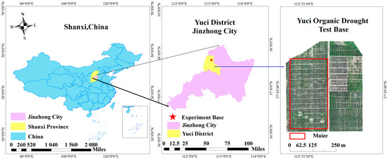
Figure 1.
Experimental location and sampling design. Study area in Lifang, Yuci District, with the 21 ground sampling sites delineated. Sample size per date and altitude: n = 21 site-level observations (mean of three replicates per site).
2.2. Data Acquisition and Preprocessing
2.2.1. Acquisition and Processing of Multispectral Data
The maize variety “Chengxin 16” was used as the experimental material, sown in mid-May 2024 and harvested on 6 October 2024. A total of 21 sampling points were established at the Lifang experimental base, Yuci District, Jinzhong City, Shanxi Province. The experimental site soil is classified as loessial soil with a loam texture. In the 0–30 cm layer, soil organic matter was 17.6 g kg−1, total nitrogen 0.98 g kg−1, and field capacity 21%. A single pre-sowing basal fertilization was applied mechanically (N–P2O5–K2O = 12–10–8 kg ha−1, as nutrient equivalents). The crop was grown under rainfed conditions with no irrigation throughout the season. UAV remote sensing flights were conducted at seven key time points: 9 June, 25 June, 4 July, 18 July, 12 August, 28 August, and 12 September 2024 (see Figure 2). At each flight, eight flight altitudes (65 m, 80 m, 100 m, 120 m, 140 m, 160 m, 180 m, and 200 m) were simultaneously set to acquire multispectral images of maize. The DJI Mavic 3 Multispectral (M3M; SZ DJI Technology Co., Ltd., Shenzhen, China) UAV data acquisition system was employed, equipped with a 4/3-inch visible light CMOS image sensor and a multispectral sensor. The acquired multispectral images comprised four spectral bands: Red (650/16 nm), Green (560/16 nm), Red Edge (RE, 730/16 nm), and Near Infrared (NIR, 860/26 nm). High-resolution multispectral images were obtained at the 65 m flight altitude under clear, cloudless weather conditions between 10:00 and 12:00 a.m. The flight was set with 70% forward overlap and 80% side overlap, accompanied by two 0.5 m × 1 m reference gray panels for reflectance calibration of the study area. Photogrammetric reconstruction of the UAV orthomosaics was performed in DJI Terra (SZ DJI Technology Co., Ltd., Shenzhen, China), and band-wise spectral reflectance was extracted using ArcGIS Desktop 10.8 (Esri, Redlands, CA, USA).
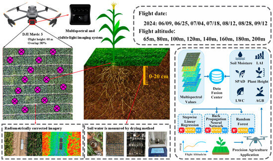
Figure 2.
Workflow of the UAV-based multispectral monitoring system.
2.2.2. Ground Data Collection
Three standard quadrats of 50 cm × 50 cm were established within the study area and precisely positioned using high-precision differential GPS (accuracy ≤ ±5 cm). Multiple key physiological and biochemical parameters of vegetation within the quadrats were systematically acquired through manual measurement protocols. To ensure data quality and reliability, all measurement instruments were calibrated using certified reference standards prior to use, with each parameter measured in triplicate and arithmetic means calculated. Outliers were identified and removed using the ±2σ criterion. The specific measured parameters included the following: relative chlorophyll content, leaf water content (LWC), leaf area index (LAI), aboveground biomass (AGB), and individual leaf area. Simultaneously, soil sampling points were deployed at 20 cm intervals within each quadrat to determine soil volumetric water content at 0–20 cm depth. All ground-truth measurements were spatially co-registered with corresponding UAV multispectral imagery pixels through geometric rectification procedures, serving as validation datasets for assessing the accuracy and reliability of remote sensing retrieval algorithms.
Canopy leaf water content was collected at sampling points, and spatial coordinates were recorded using a handheld RTK device. Plant leaves were detached and labeled, the fresh weight was measured, then leaves were placed in an oven at 105 °C for 30 min to kill enzymes, followed by drying at 80 °C until at a constant weight, and the dry weight was measured to calculate leaf water content according to (Equation (1)).
where represents the leaf water content; represents the fresh weight of the leaf; and represents the dry weight of the leaf.
At the sampling points, the soil mass water content in the 0–20 cm soil layer was determined using the soil auger method and oven-drying weighing method (Equation (2)), and the soil bulk density in the 0–20 cm soil layer was measured using the ring cutter method (Equation (3)). Three replicates were taken for each layer, with each 10 cm considered as one layer within the 0–20 cm depth.
where is the soil mass water content (g/g), is the weight of the aluminum box (g), is the total weight of the aluminum box and wet soil (g), and is the total weight of the aluminum box and dry soil (g).
The gravimetric water content is converted to volumetric water content (Equation (4)).
where is the soil bulk density (g·cm3); is the weight of the ring cutter with dry soil (g); is the weight of the ring cutter (g); is the volume of the ring cutter (cm3); and is the soil volumetric water content (%).
At each sampling point, a SPAD-502 handheld chlorophyll meter was used to measure the SPAD value of 1–2 canopy leaves around the crops. Five measurements were taken at the leaf base, middle, and tip, respectively, for each leaf, and the average of these three positions was taken as the SPAD value of the leaf. The mean of all measured leaves was calculated as the representative chlorophyll value for the sampling point.
The leaf area was obtained by collecting all leaves from sampled plants, counting the number, flattening them under a glass plate, and photographing them from above, together with a ruler. The actual leaf area was extracted by processing the images with the ArcGIS Desktop 10.8 (Esri, Redlands, CA, USA), and the leaf length, width, and calibrated area were combined to calculate the leaf area coefficient. The crop density within 1 m2 was also recorded in the field to estimate the LAI.
Three plants with similar growth status were selected around each sampling point, uprooted entirely, placed into fresh-keeping bags, and brought back to the laboratory promptly. Roots, stems, leaves, and fruits were separated and weighed. Each part was placed in mesh bags, heated at 105 °C for 30 min to kill enzymes, then dried at 80 °C for 24 h until at a constant weight, to measure the biomass of each plant. The average biomass per plant was calculated for each sampling point, and the total biomass per sampling point was estimated based on the plant density within 1 m2 (kg/m2).
The plant height was measured from the ground to the highest point of the plant. At each sampling point, three plants with similar growth status were selected, measured, and the average value was taken.
2.2.3. Spectral Indices
Vegetation indices are dimensionless indicators based on multispectral or hyperspectral data, primarily derived by combining the reflectance of vegetation across different spectral bands to extract key information about the vegetation, thereby reflecting various vegetation parameters. This study calculated multiple vegetation indices (Table 1) using the previously extracted multispectral bands and employed these vegetation indices to build monitoring models for soil moisture, crop SPAD, plant height, LAI, aboveground biomass (AGB), and leaf water content (LWC).

Table 1.
Vegetation indices used in this study.
2.3. Model Construction and Evaluation
This study employs three algorithms—stepwise linear regression (SLR), random forest (RF), and back-propagation neural networks (BPNNs)—to represent distinct modeling paradigms. (1) SLR serves as a baseline traditional statistical approach with strong interpretability; (2) RF, a canonical ensemble method, effectively handles high dimensionality and feature interactions; and (3) BPNN, as a deep-learning method, captures complex nonlinear relationships. The selection reflects a balance between computational efficiency and practical deployability, a trade-off between model complexity and interpretability, and the algorithms’ established use in multispectral vegetation-parameter retrieval. This trio enables a comprehensive assessment across linear, ensemble, and neural paradigms while maintaining operational feasibility for real-world monitoring. We further posit the following hypotheses: machine-learning models (RF and BPNN) will achieve significantly higher retrieval accuracy than traditional linear regression, particularly when modeling the nonlinear relationships inherent in multispectral data; moreover, different vegetation parameters exhibit distinct sensitivities to multispectral indices. The experiments were conducted on a workstation running Windows 11, equipped with an Intel i7-12700 processor, an NVIDIA RTX 3060 GPU, and 32 GB of RAM.
2.3.1. Correlation Analysis
This study conducted a correlation analysis using the Pearson correlation coefficient method [51]. Correlation analysis is used to investigate the relationships among multiple variables, assessing whether there is an association between variables as well as the strength and direction of such associations. The results of correlation analysis help the understanding of the mutual influence among variables and provide a basis for data analysis and model construction.
2.3.2. Stepwise Linear Regression
Stepwise linear regression [52] is a method that optimizes the regression equation by gradually selecting and adjusting independent variables (X). This method introduces key variables into the model one by one based on their significant influence on the dependent variable (Y) and tests the variables already included. Variables that become insignificant due to the inclusion of new variables will be removed. The significance test ensures that the final model contains only effective variables that have a significant impact on the dependent variable, thereby avoiding interference from invalid variables.
2.3.3. Random Forest
Random forest [53] is an ensemble learning algorithm mainly used for classification and regression tasks. It consists of multiple decision trees. In classification, the random forest determines the final result by majority voting; in regression, it takes the average of outputs. By combining the results of multiple trees, it improves the accuracy and stability of the model. Random forest performs well in handling nonlinear data and complex feature interactions and can effectively reduce the risk of overfitting.
2.3.4. BP Neural Network
The BP neural network [54] is a multilayer feedforward neural network trained using the error back-propagation algorithm. It consists of an input layer, hidden layers, and an output layer. By propagating data layer by layer and back-propagating errors to each layer, weights are adjusted to gradually approach the optimal solution. BP neural networks excel in handling complex nonlinear problems and are widely applied in pattern recognition, regression analysis, and classification tasks.
2.3.5. Model Validation and Evaluation
With the independent holdout test set fixed, we conducted 5-fold cross-validation on the training split and evaluated performance using the correlation coefficient (R), coefficient of determination (R2), root mean square error (RMSE), and relative error (RE). Additionally, to mitigate spatial bias, the baseline homogeneity across the 21 sampling points was assessed.
The correlation coefficient R [55] is a statistic that measures the strength and direction of the linear relationship between two variables, ranging from −1 to 1. A positive value indicates positive correlation, and a negative value indicates negative correlation. Significance tests of R were conducted between vegetation indices and crop phenotypic parameters, including SPAD, plant height, LAI, AGB, and LWC. Values closer to 1 or −1 indicate a stronger correlation between variables.
The coefficient of determination (Equation (5)) represents the explanatory power of independent variables on the dependent variable and reflects the goodness of fit of the model [55]. The value of R2 ranges from 0 to 1; the higher the value, the stronger the model’s explanatory power for the data.
where is the true value of the sample, is the measured value of the sample, is the average of the true values, and is the number of samples.
Relative error (Equation (6)) is a measure used to quantify the deviation of measured values from true values, serving to evaluate the accuracy and reliability of the model [56]. Relative error better reflects the model’s credibility; a smaller RE indicates more accurate measurement results. The calculation formula is as follows:
where is the number of samples, and and are the measured value and true value of the th sample, respectively.
Root mean square error (RMSE) (Equation (7)) is a statistical indicator used to measure the error between measured values and actual values [56]. It reflects the accuracy and stability of the model monitoring. A smaller RMSE value indicates a smaller difference between measured and actual values. The calculation formula is as follows:
where is the number of samples, and and are the measured value and true value of the th sample, respectively.
3. Results
3.1. Correlation Analysis Between Vegetation Indices at Different Heights and Soil Moisture and Phenotypic Parameters of Maize
Homogeneity tests confirmed that baseline conditions were consistent across the 21 sampling points (no significant differences, p > 0.05). Figure 3 shows the Pearson correlation analysis results between 24 vegetation indices at different altitudes and soil moisture at 0–20 cm depth. Most vegetation indices exhibit a negative correlation with soil moisture. Vegetation indices significantly correlated with soil moisture at the 0.01 significance level were selected as modeling factors (Table 2). Based on 16 vegetation indices at different flight altitudes, Pearson correlation analyses were conducted for chlorophyll, leaf water content, leaf area index, plant height, and biomass. Vegetation indices significantly correlated with each indicator at the 0.01 significance level were selected as modeling factors (Table 2).
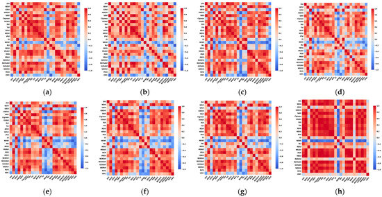
Figure 3.
Correlations between vegetation indices and 0–20 cm soil moisture at eight flight altitudes. (a) 65 m; (b) 80 m; (c) 100 m; (d) 120 m; (e) 140 m; (f) 160 m; (g) 180 m; (h) 200 m.
Table 2.
Vegetation indices selected based on significance for modeling maize soil moisture and phenotypic parameters.
Based on different flight altitudes (65–200 m), the modeling performance of multiple vegetation indices for maize soil moisture and phenotypic parameters (SPAD, leaf water content, leaf area index, plant height, and aboveground biomass) was systematically evaluated (Table 2). According to the variations in correlation coefficients and sensitivity characteristics, the flight altitudes were divided into low-altitude (65–100 m), mid-altitude (120–160 m), and high-altitude (180–200 m) ranges.
In the low-altitude range (65–100 m), maize soil moisture and various phenotypic parameters exhibited extremely high sensitivity to mainstream vegetation indices. Specifically, the correlation coefficients between soil moisture and indices such as NLI, DVI, and NDGI reached as high as −0.754 to −0.793, all passing the 0.01 significance level test, demonstrating the superiority of low-altitude remote sensing for soil moisture inversion. Within this altitude range, SPAD showed correlations exceeding 0.82 (up to 0.858) with NDVI, GNDVI, and other indices, significantly higher than at other altitudes. LWC also showed the strongest correlations with NDVI, GNDVI, and similar indices in the 65–100 m range (r = 0.803–0.809), with the combined indices TVI, GNDVI, NDVI, and RVI at 80 m providing the greatest explanatory power for LWC. LAI reached peak correlations with NDVI, GNDVI, and other indices between 80 and 100 m (up to 0.897), while AGB showed strong correlations with GNDVI, NDVI, OSAVI, NLI, and GRVI in the low-altitude range. Overall, low-altitude remote sensing achieved the highest inversion accuracy for maize phenotypic and biomass parameters.
The mid-altitude range (120–160 m) achieved a balance between modeling accuracy and remote sensing coverage. Although correlations between phenotypic parameters and vegetation indices were slightly lower than those in the low-altitude range, most remained at relatively high levels. At 120 m and 140 m, soil moisture still exhibited correlation coefficients above −0.75 with NDGI, NLI, GI, DVI, and GRVI, indicating strong modeling stability. SPAD and LWC maintained correlations with NDVI and GNDVI in the range of 0.674–0.804, with 140 m performing the best. Plant height showed correlations of 0.631–0.665 with GNDVI, NDVI, and OSAVI, while AGB correlations slightly decreased but remained around 0.588. This altitude range is suitable for remote sensing applications at the field scale.
At high altitudes (180–200 m), the overall correlations between phenotypic parameters and vegetation indices decreased, and inversion sensitivity was markedly weakened. Soil moisture correlations with major vegetation indices dropped to −0.643 and −0.589, while SPAD maintained a correlation of 0.553 with GNDVI, but was notably lower than in the low- and mid-altitude ranges. LWC, LAI, plant height, and AGB generally showed correlations in the range of 0.4–0.6 with various indices at this altitude, with some parameters (e.g., NDVI for AGB) dropping to 0.402. This indicates that high-altitude remote sensing has limited accuracy and sensitivity for the inversion of maize phenotypic and biomass parameters.
Overall, across flight altitudes, correlations between parameters and vegetation indices were generally higher in the low-altitude range (65–140 m) than in the mid- and high-altitude ranges, showing stronger index sensitivity. NDVI, GNDVI, NLI, and OSAVI demonstrated good generality and adaptability for multiple phenotypic parameters and can be prioritized for maize phenotypic parameter remote sensing modeling. Moreover, parameter sensitivity to flight altitude varied: SPAD and LAI responded more markedly to altitude changes, while AGB and soil moisture correlations were more strongly affected by flight altitude. All correlations reached significant or highly significant levels (p < 0.01), indicating that optimizing the combination of flight altitude and vegetation indices is of great importance for improving the inversion accuracy of maize soil moisture and phenotypic parameters, and the choice of flight platform altitude and index type should be made according to application needs.
3.2. Inversion of Maize Soil Moisture and Phenotypic Parameters Based on Three Models
Figure 4 compares the modeling performance of three methods—stepwise linear regression, random forest (RF), and back-propagation neural network (BP)—for soil moisture and maize phenotypic parameters (b. SPAD, c. leaf water content (LWC), d. leaf area index (LAI), e. plant height, and f. aboveground biomass (AGB)) at different flight altitudes (65–200 m). Each subplot presents the variation of evaluation metrics, including the coefficient of determination (R2), root mean square error (RMSE), and relative error (RE), with the flight altitude and modeling method, in the form of polar annular charts.
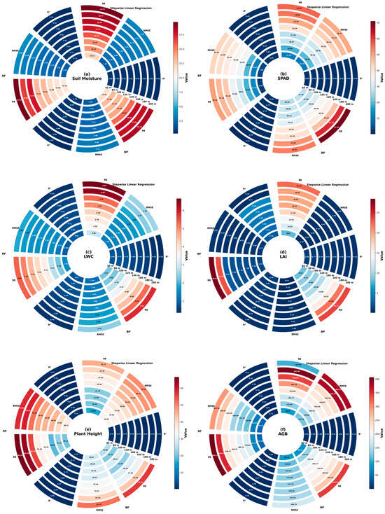
Figure 4.
Performance of SLR, RF, and BPNN across flight altitudes for six targets. (a) Soil moisture; (b) SPAD; (c) leaf water content; (d) leaf area index; (e) plant height; (f) aboveground biomass.
Overall, the modeling performance of different parameters shows significant differences. The low-altitude range (65–100 m) generally achieves higher R2 values and lower RMSE and RE, while the inversion accuracy decreases with increasing flight altitude. Taking soil moisture and SPAD as examples, all three methods reached R2 values above 0.6 in the low-altitude range, with RMSE and RE significantly lower than those at high altitudes, demonstrating higher inversion accuracy. Leaf water content and LAI showed the best inversion performance in the 80–120 m range, with R2 peaks exceeding 0.65 and the lowest RMSE and RE. The overall inversion accuracy of plant height and aboveground biomass was relatively low, especially in the high-altitude range of 180–200 m, where R2 values were generally below 0.5 and RMSE and RE increased.
From the comparison of different modeling methods, random forest (RF) and the BP neural network generally achieved higher R2 values and lower error metrics (RMSE and RE) than stepwise linear regression for most parameter–altitude combinations. The BP model performed best in the inversion of leaf area index and aboveground biomass, reflecting its strong adaptability to nonlinear relationships. The stepwise linear regression method was more affected by altitude and data complexity, with notable fluctuations in accuracy. The inversion capability of the three modeling methods at different flight altitudes showed a strong dependence on altitude, with low-altitude remote sensing being more suitable for high-accuracy inversion of multiple maize parameters. Random forests and back-propagation neural networks (BPNNs) demonstrate superior stability and generalization performance; this performance differential is consistent with the findings of Dey et al. [57], further indicating that machine-learning approaches exhibit greater robustness than traditional linear models in agricultural applications.
3.3. Analysis of Differences in Inversion Results
Figure 5 shows the variation trends of the coefficient of determination (R2), root mean square error (RMSE), and relative error (RE) with altitude for the optimal modeling schemes of maize soil moisture and five phenotypic parameters (SPAD, leaf water content (LWC), leaf area index (LAI), plant height, and aboveground biomass (AGB)) at different flight altitudes (65–200 m).
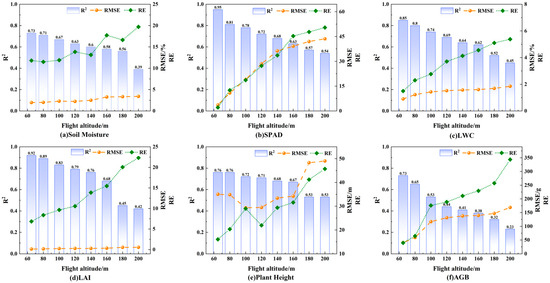
Figure 5.
Variations of optimal modeling and R2, RMSE, and RE for maize soil moisture and phenotypic parameters at different flight altitudes. (a) Soil moisture; (b) SPAD; (c) leaf water content; (d) leaf area index; (e) plant height; (f) aboveground biomass.
From the variation in R2 for each parameter, all traits achieved higher goodness-of-fit in the low-altitude range (65–100 m), with R2 generally exceeding 0.70. Among them, LAI and SPAD reached R2 values above 0.92 and 0.86, respectively, while soil moisture, LWC, plant height, and AGB reached values as high as 0.73, 0.85, 0.76, and 0.73, respectively. As the flight altitude increased, R2 showed a continuous decline, and by 200 m, the R2 values for all parameters had dropped significantly (down to as low as 0.23), indicating reduced modeling accuracy for high-altitude remote sensing.
In terms of error metrics, both RMSE and RE increased with altitude. The low-altitude range had smaller RMSE and RE values, indicating good modeling accuracy. For example, LAI, SPAD, and LWC at 80–100 m recorded the lowest RMSE and RE values, as low as 0.05, 10.37, and 0.67, respectively, with RE also maintained at a low level. As the altitude increased to 200 m, RMSE and RE rose sharply, reflecting that high-altitude data are more affected by factors such as mixed ground objects and reduced spatial resolution, leading to significantly higher prediction errors.
All traits achieved optimal modeling performance in the low-altitude range (65–100 m), while the model explanatory power and prediction accuracy declined markedly with increasing altitude. This result indicates that low-altitude remote sensing platforms are more suitable for high-accuracy inversion and quantitative monitoring of maize soil moisture and key phenotypic parameters, providing data support for precision agriculture management and the selection of high-throughput phenotyping platforms.
3.4. Spatial Distribution of Inversion Results
On July 10, maize was in the jointing to big trumpet stage, the period of fastest growth and greatest spatial heterogeneity, making it a critical period for reflecting the soil–crop spatiotemporal pattern and model capability. To reveal the spatial distribution characteristics of maize soil moisture and phenotypic parameter monitoring using UAV multispectral remote sensing imagery at different flight altitudes, this study presents the spatial prediction results of six indicators—soil moisture (a), SPAD (b), leaf water content (LWC, c), leaf area index (LAI, d), plant height (e), and aboveground biomass (AGB, f)—at flight altitudes ranging from 65 m to 200 m, using three modeling methods: random forest (RF), BP neural network (BPNN), and stepwise regression (STEP) (see Figure 6).
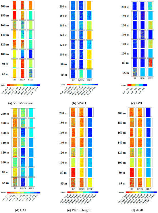
Figure 6.
Spatial maps of inverted parameters at multiple flight altitudes on 10 July. (a) Soil moisture; (b) SPAD; (c) leaf water content; (d) leaf area index; (e) plant height; (f) aboveground biomass.
In the low-altitude range (65–100 m), model prediction results exhibited strong spatial heterogeneity and rich detail, effectively reflecting subtle variations and actual distributions of maize soil moisture and phenotypic parameters within the plots. Especially under the RF and BPNN models, the spatial distribution layers of soil moisture, SPAD, LAI, and other phenotypic parameters showed higher resolution and coherence, demonstrating the advantages of low-altitude remote sensing in high-accuracy quantitative monitoring.
As the flight altitude increased to the mid-altitude range (120–160 m), the spatial distributions of parameters displayed a certain homogenization trend, with gradual loss of local details and moderate reduction in inter-plot differences; however, the main spatial variation patterns were still accurately captured, meeting the requirements for regional-scale phenotypic monitoring. Among them, the BPNN model showed a stronger ability to preserve spatial variation, with prediction layers still presenting noticeable spatial gradients and differences.
At high altitudes (180–200 m), spatial distributions of all parameters under the three models tended to become smoother, with obvious loss of local information. This was especially pronounced in the stepwise regression (STEP) model, where spatial details were severely insufficient, and prediction layers appeared as large uniform patches, making it difficult to identify subtle differences within the fields. Although RF and BPNN models partially preserved spatial structures, their overall resolution was lower, reflecting the applicability of high-altitude remote sensing data for coarse, large-scale monitoring and highlighting its spatial resolution limitations.
Sensitivity to modeling methods and flight altitude also varied among the indicators. Soil moisture and LWC showed a more pronounced reduction in spatial variability at high altitudes, while phenotypic parameters such as LAI and AGB exhibited the most detailed spatial distribution at low altitudes. Overall, low-altitude remote sensing combined with RF and BPNN models can better restore the true spatial heterogeneity within maize fields, making it suitable for high-precision and precise monitoring; the mid-altitude range is appropriate for regional-scale applications, balancing efficiency and accuracy; and the high-altitude range is more suitable for coarse, large-scale dynamic monitoring.
4. Discussion
4.1. Effects of Flight Altitude on Vegetation Index Sensitivity and Model Inversion Accuracy
This study revealed the significant impact of UAV flight altitude on the sensitivity of multispectral vegetation indices and the inversion accuracy of crop phenotypic parameters. In the low-altitude range (65–100 m), soil moisture showed correlation coefficients with NLI, DVI, NDGI, and other vegetation indices ranging from −0.754 to −0.793, while maize SPAD correlated with NDVI and GNDVI above 0.816, significantly higher than those at mid- and high-altitude ranges. This phenomenon is attributed to the flight altitude directly determining the spatial resolution of imagery and the degree of spectral mixing of ground objects. Jin et al. [58] confirmed this pattern, finding that ultra-low-altitude UAV imagery at 30 m achieved a high accuracy of R2 = 0.89 in estimating wheat plant density, whereas traditional satellite remote sensing only reached R2 = 0.65. This result is highly consistent with the R2 = 0.92 inversion accuracy of LAI in the low-altitude range in this study. The advantage of low-altitude remote sensing lies in its higher spatial resolution, which reduces mixed pixel effects, making individual pixels closer to pure pixels and more accurately reflecting the spectral characteristics of target crops [59]. Meanwhile, the shorter atmospheric path decreases the impact of atmospheric scattering and absorption on spectral signals, improving spectral measurement accuracy [60].
Regarding quantifying resolution/SNR loss with altitude, with identical optics, the ground sampling distance (GSD) scales linearly with altitude. Moving from 65 m to 200 m enlarges the pixel footprint by 3.08 in length and 9.5 in area. Hence, the number of pixels per unit ground area decreases by 90%, sharply increasing the probability of vegetation–soil mixing and weakening the delineation of vegetation–soil boundaries that many VIs rely on. A longer atmospheric path at higher altitudes also reduces the effective signal-to-noise ratio for canopy signals. These scale/SNR effects explain the observed accuracy drop at high altitude.
Different phenotypic parameters exhibited varied sensitivity responses to changes in flight altitude. LAI and SPAD, as key indicators reflecting crop canopy density and chlorophyll content, were the most sensitive to spatial resolution changes. Their inversion accuracies dropped to 0.23 and 0.55, respectively, at the 200 m high-altitude range, representing a decline of over 75% compared to the low-altitude range. This difference mainly stems from the distinct spectral response mechanisms of the parameters. LAI primarily influences near-infrared reflectance through vegetation coverage and requires precise delineation of vegetation–soil boundaries. SPAD regulates absorption depth in the red light band through chlorophyll content, demanding very high spectral accuracy [36]. In contrast, structural parameters such as aboveground biomass and plant height showed relatively lower sensitivity to altitude changes, possibly due to their multispectral integrated response characteristics. Gevaert et al. [61] observed similar patterns in multi-scale remote sensing studies, confirming that structural parameters exhibit stronger scale stability. Notably, a threshold effect emerged: when the altitude exceeded 120 m, the inversion accuracy for all traits began to decline; beyond 160 m, the decline accelerated. This operational threshold is consistent with the transition from sub-meter to coarser effective resolutions and provides actionable guidance for flight planning.
Regarding the rationale for the selected set of 24 vegetation indices, the indices were chosen a priori to span complementary mechanisms pertinent to the six target variables (SM, SPAD, LWC, LAI, PH, and AGB), including classic vigor/chlorophyll metrics (e.g., NDVI, GNDVI, and GRVI), soil-adjusted formulations that attenuate background effects under sparse canopies (e.g., SAVI, OSAVI, and MSAVI), water/green-band-enhanced indicators sensitive to leaf water status and canopy “greenness” (e.g., NDWI, NDGI, and Clgreen), red-edge or derivative constructs that capture subtle biochemical and structural variation (e.g., RERDVI and REOSAVI), and contrast/difference measures that are responsive to coverage and illumination variability (e.g., DVI, RDVI, and WDVI). Collectively, this ensemble aligns with established practice in agricultural remote sensing, provides sensitivity across a range of canopy-cover conditions, and preserves comparability with prior studies.
4.2. Adaptability Differences of Various Models for the Inversion of Maize Soil Moisture and Phenotypic Parameters
Comparing stepwise linear regression (SLR), random forest (RF), and BP neural network (BP) revealed clear differences in algorithm adaptability to UAV multispectral data. Machine-learning methods significantly outperformed traditional statistical methods across most trait–altitude cells: RF and BP generally achieved R2 values 0.15–0.35 higher than SLR and reduced RMSE by 20–40%. RF showed strong stability and generalization, especially for high-dimensional multispectral inputs; its bootstrap sampling and random feature selection help it avoid overfitting, capture complex interactions, and remain robust to outliers and noise [62,63]. BP performed best for LAI and AGB due to its nonlinear mapping capacity; similar benefits of deep neural models for vegetation-index/biophysical relations have been reported in crop-yield prediction [64]. Our excellent BP performance for LAI (R2 = 0.92) supports this finding. In contrast, SLR—though interpretable—rests on linear assumptions often violated in crop–environment systems and becomes less stable as the data distribution shifts with altitude; reviews of biophysical inversion further highlight the curse of dimensionality and collinearity that limit linear methods with modern spectral data [65].
As application-oriented recommendations, for time-critical or regional operations prioritizing robustness and computational efficiency, RF is preferable; for scientific analyses seeking peak accuracy, BP is recommended; and for management scenarios requiring transparent reasoning, RF with feature-importance analysis offers interpretability while retaining good accuracy [66].
4.3. Flight Strategies
Based on the above accuracy–efficiency analysis, we propose a differentiated flight-strategy framework. A low altitude (65–100 m) is recommended for field-scale precision management: within this range, LAI/SPAD/LWC errors meet high-precision information needs, consistent with prior evidence that low-altitude imaging delivers fine within-field variation [67,68]. The mid-altitude distances (120–160 m) provide the best balance between accuracy and efficiency for regional monitoring; although correlations decline compared with 65–100 m, most remain between 0.6 and 0.8, satisfying regional decision needs, in line with reviews that moderate altitudes suit large-scale crop monitoring [29]. A high altitude (180–200 m) supports rapid reconnaissance: although the inversion accuracy is lower, the wide swath and high efficiency are advantageous for macro-level tasks such as resource surveys, crop-structure mapping, and disaster assessment [69].
In practical applications, we recommend a hierarchical multi-altitude operational framework, progressing from high-altitude synoptic reconnaissance to mid-altitude regional monitoring, and ultimately to low-altitude fine-scale diagnostic mapping [16]. This workflow aligns with the operational needs of producers of different scales and provides flexible service options. Our improvements in model accuracy directly support two core management decisions. (1) The first is irrigation scheduling. Low-altitude (65–100 m) maps of soil moisture (SM) and leaf water content (LWC) enable delineation of within-field water-deficit zones; combined with site-specific thresholds calibrated to the soil texture and phenological stage, the continuous surfaces are converted into binary or multi-class irrigation prescriptions. Mid-altitude (120–160 m) acquisitions are then used for post-irrigation assessment and regional prioritization. (2) The second is precision fertilization. Low-altitude SPAD/LAI maps provide early diagnosis of nitrogen deficiency; quantile-based or agronomically calibrated cut-offs are applied to derive variable-rate application zones. RF is preferred for robust, time-critical operational products, whereas BP is suited when maximal diagnostic accuracy is required. A “calibration → mapping → zonation → prescription export → post-treatment verification” workflow links retrieval accuracy directly to executable irrigation and fertilization actions.
4.4. Insights, Limitations, and Future Directions
This study provides multiple important insights for the scientific application of UAV-based agricultural remote sensing. First, flight altitude selection should be scientifically configured based on specific application needs. Machine-learning methods demonstrate clear advantages in processing multispectral remote sensing data and have become the preferred technology for agricultural remote sensing modeling. Differentiated flight strategies can better meet the diverse demands of agricultural operators of varying scales and types, facilitating the widespread adoption of UAV technology [70]. This study also highlights the importance of standardization in UAV remote sensing, as establishing unified operational protocols and quality standards is crucial for ensuring data quality and enhancing application effectiveness. Tsouros et al. [18], in their review of UAV applications in precision agriculture, similarly emphasized the significance of technological standardization for industry development. The proposed flight strategy framework can provide a scientific basis for the formulation of related standards. With respect to the models’ interannual transferability and representativeness, our generalization is founded on physically based, altitude-dependent scaling laws; as the flight height increases, the ground-sampling distance (GSD) increases approximately linearly, while the effective canopy signal-to-noise ratio (SNR) diminishes. Because these mechanisms are independent of interannual variability, the direction and relative ordering of altitude effects on retrieval accuracy are expected to be transferable across seasons and comparable agro-ecological settings. Nevertheless, absolute accuracy metrics may vary with background conditions and meteorological regimes; accordingly, site- and season-specific calibration is recommended prior to large-scale deployment.
Despite these advances, some limitations remain that warrant improvement in future research. These mainly include spatiotemporal scale constraints: this study was conducted at a single experimental site and focused on a specific growth stage of maize. Soil backgrounds, climate conditions, crop varieties, and management practices in different regions may influence the flight altitude effects observed. Hassler and Baysal-Gurel [71] pointed out that UAV agricultural applications need to consider regional differences and crop specificity. Environmental factors were insufficiently considered; factors such as illumination conditions, atmospheric transparency, and wind speed received relatively little attention. Aasen et al. [59] emphasized the important impact of environmental conditions on UAV spectral data quality. Limitations in sensor technology and the complexity of optimizing operational parameters also require further investigation. This study focuses on quantifying the effect of flight altitude on retrieval accuracy; therefore, we do not enumerate, in the main text, regression coefficients and RF/BPNN feature-importance rankings for every altitude–trait–index combination. Likewise, although we report descriptive comparisons of R2, RMSE, and RE, we did not perform an exhaustive set of across-model significance tests for each altitude–trait cell, nor a full band/index-level sensitivity analysis, so as to remain within scope and avoid excessive length. In subsequent work, we will provide formal statistical comparisons together with a multi-model sensitivity analysis to identify which bands/indices contribute most to performance at each altitude.
Future research should prioritize multi-region and multi-crop validation across climatic zones, soil types, and varieties; joint optimization of operational parameters (altitude, speed, overlap, and sensor settings) [72]; and integration of intelligent technologies (edge computing and AI) to enable real-time processing and decision support [73]. Establishing standardized frameworks and testing novel sensors will further advance UAV agricultural remote sensing [74].
5. Conclusions
Flight altitude is a primary determinant of UAV multispectral retrieval performance. Low-altitude deployments yield the highest retrieval accuracy for trait-level diagnostics; mid-altitude deployments provide the most favorable accuracy–efficiency trade-off for regional management; and high-altitude deployments maximize areal coverage for rapid synoptic reconnaissance. Across parameter–altitude settings, machine-learning models (RF/BP) consistently surpass linear baselines: RF affords an advantageous balance among accuracy, computational efficiency, and interpretability for operational products, whereas BP tends to deliver the highest accuracy for vegetation-structure traits.
On the basis of these findings, we advance the following operational recommendations. (1) Altitude should be decided by objective—use ≤100 m for fine-scale diagnostic mapping, 120–160 m for regional monitoring, and 180–200 m for rapid reconnaissance. (2) Models should be chosen by task—use RF for time-critical, region-scale products and BP for accuracy-oriented scientific analyses, with RF feature-importance supporting interpretability. (3) A hierarchical workflow should be used—progress from high-altitude synoptic reconnaissance to mid-altitude regional monitoring, and finally to low-altitude fine-scale diagnostic mapping. Implemented within standardized operating procedures, these recommendations provide actionable guidance for scalable agricultural UAV remote-sensing services and inform the development of relevant technical standards and industry practice. Low-altitude SM/LWC and SPAD/LAI products underpin irrigation prescriptions and variable-rate N topdressing, respectively; mid-altitude updates support regional ranking and verification. Exporting these geospatial products as prescription maps closes the loop from remote-sensing retrievals to in-field operations.
Author Contributions
Conceptualization, Y.L., S.G. and Y.Y.; methodology, Y.L., S.G. and S.J.; software, Y.L., S.J. and S.G.; formal analysis, Y.L., Y.Y. and S.G.; data curation, Y.L., S.G. and S.J.; writing—original draft preparation, Y.L., H.J., S.G. and W.Z.; writing—review and editing, Y.L., H.J. and W.Z.; visualization, Y.Y. and H.J.; supervision, W.Z.; project administration, W.Z.; funding acquisition, W.Z. All authors have read and agreed to the published version of the manuscript.
Funding
This work was supported by the Postgraduate Education Innovation Program of Shanxi Province [2024KY293]; the Science and Technology Major Project of Shanxi Province, China [202202140601021]; the National Key Research and the Development Program of China [2021YFD1901101]; and the Science and Technology Major Project of Shanxi Province, China [202101140601026].
Data Availability Statement
The data presented in this study are available on request from the corresponding author due to the ongoing related research project and institutional policy.
Conflicts of Interest
The authors declare no conflicts of interest.
References
- Shiferaw, B.; Prasanna, B.M.; Hellin, J.; Bänziger, M. Crops that feed the world 6. Past successes and future challenges to the role played by maize in global food security. Food Secur. 2011, 3, 307–327. [Google Scholar] [CrossRef]
- Aldrighettoni, J.; D’Urso, M.G. Advances in Precision Farming: A contribute for estimating crop health and water stress by comparing UAV Multispectral and Thermal Imagery. ISPRS Ann. Photogramm. Remote Sens. Spat. Inf. Sci. 2025, 33–40. [Google Scholar] [CrossRef]
- Mohanty, B.P.; Cosh, M.H.; Lakshmi, V.; Montzka, C. Soil moisture remote sensing: State-of-the-science. Vadose Zone J. 2017, 16, 1–9. [Google Scholar] [CrossRef]
- Singhal, G.; Bansod, B.; Mathew, L.; Goswami, J.; Choudhury, B.; Raju, P. Chlorophyll estimation using multi-spectral unmanned aerial system based on machine learning techniques. Remote Sens. Appl. Soc. Environ. 2019, 15, 100235. [Google Scholar] [CrossRef]
- Li, Y.; Qu, T.; Wang, Y.; Zhao, Q.; Jia, S.; Yin, Z.; Guo, Z.; Wang, G.; Li, F.; Zhang, W. UAV-Based Remote Sensing to Evaluate Daily Water Demand Characteristics of Maize: A Case Study from Yuci Lifang Organic Dry Farming Experimental Base in Jinzhong City, China. Agronomy 2024, 14, 729. [Google Scholar] [CrossRef]
- Wang, X.; Ren, J.; Wu, P. Analysis of Growth Variation in Maize Leaf Area Index Based on Time-Series Multispectral Images and Random Forest Models. Agronomy 2024, 14, 2688. [Google Scholar] [CrossRef]
- Han, L.; Yang, G.; Dai, H.; Xu, B.; Yang, H.; Feng, H.; Li, Z.; Yang, X. Modeling maize above-ground biomass based on machine learning approaches using UAV remote-sensing data. Plant Methods 2019, 15, 10. [Google Scholar] [CrossRef]
- Gang, S.; Wenjiang, H.; Pengfei, C.; Shuai, G.; Xiu, W. Advances in UAV-based multispectral remote sensing applications. Nongye Jixie Xuebao/Trans. Chin. Soc. Agric. Mach. 2018, 49, 1–17. [Google Scholar]
- Cheng, M.; Sun, C.; Nie, C.; Liu, S.; Yu, X.; Bai, Y.; Liu, Y.; Meng, L.; Jia, X.; Liu, Y. Evaluation of UAV-based drought indices for crop water conditions monitoring: A case study of summer maize. Agric. Water Manag. 2023, 287, 108442. [Google Scholar] [CrossRef]
- Ge, H.; Zhang, Q.; Shen, M.; Qin, Y.; Wang, L.; Yuan, C. Enhancing yield prediction in maize breeding using UAV-derived RGB imagery: A novel classification-integrated regression approach. Front. Plant Sci. 2025, 16, 1511871. [Google Scholar] [CrossRef]
- Awais, M.; Li, W.; Cheema, M.; Zaman, Q.; Shaheen, A.; Aslam, B.; Zhu, W.; Ajmal, M.; Faheem, M.; Hussain, S. UAV-based remote sensing in plant stress imagine using high-resolution thermal sensor for digital agriculture practices: A meta-review. Int. J. Environ. Sci. Technol. 2023, 20, 1135–1152. [Google Scholar] [CrossRef]
- Gago, J.; Douthe, C.; Coopman, R.E.; Gallego, P.P.; Ribas-Carbo, M.; Flexas, J.; Escalona, J.; Medrano, H. UAVs challenge to assess water stress for sustainable agriculture. Agric. Water Manag. 2015, 153, 9–19. [Google Scholar] [CrossRef]
- Colomina, I.; Molina, P. Unmanned aerial systems for photogrammetry and remote sensing: A review. ISPRS J. Photogramm. Remote Sens. 2014, 92, 79–97. [Google Scholar] [CrossRef]
- Maes, W.H.; Steppe, K. Perspectives for remote sensing with unmanned aerial vehicles in precision agriculture. Trends Plant Sci. 2019, 24, 152–164. [Google Scholar] [CrossRef]
- Adedeji, O.; Abdalla, A.; Ghimire, B.; Ritchie, G.; Guo, W. Flight Altitude and Sensor Angle Affect Unmanned Aerial System Cotton Plant Height Assessments. Drones 2024, 8, 746. [Google Scholar] [CrossRef]
- Guan, S.; Fukami, K.; Matsunaka, H.; Okami, M.; Tanaka, R.; Nakano, H.; Sakai, T.; Nakano, K.; Ohdan, H.; Takahashi, K. Assessing Correlation of High-Resolution NDVI with Fertilizer Application Level and Yield of Rice and Wheat Crops Using Small UAVs. Remote Sens. 2019, 11, 112. [Google Scholar] [CrossRef]
- Sun, Z.; Wang, X.; Wang, Z.; Yang, L.; Xie, Y.; Huang, Y. UAVs as remote sensing platforms in plant ecology: Review of applications and challenges. J. Plant Ecol. 2021, 14, 1003–1023. [Google Scholar] [CrossRef]
- Tsouros, D.C.; Bibi, S.; Sarigiannidis, P.G. A review on UAV-based applications for precision agriculture. Information 2019, 10, 349. [Google Scholar] [CrossRef]
- Liu, Q.; Wu, Z.; Cui, N.; Jin, X.; Zhu, S.; Jiang, S.; Zhao, L.; Gong, D. Estimation of soil moisture using multi-source remote sensing and machine learning algorithms in farming land of Northern China. Remote Sens. 2023, 15, 4214. [Google Scholar] [CrossRef]
- Liu, S.; Jin, X.; Nie, C.; Wang, S.; Yu, X.; Cheng, M.; Shao, M.; Wang, Z.; Tuohuti, N.; Bai, Y. Estimating leaf area index using unmanned aerial vehicle data: Shallow vs. deep machine learning algorithms. Plant Physiol. 2021, 187, 1551–1576. [Google Scholar] [CrossRef]
- Gano, B.; Bhadra, S.; Vilbig, J.M.; Ahmed, N.; Sagan, V.; Shakoor, N. Drone-based imaging sensors, techniques, and applications in plant phenotyping for crop breeding: A comprehensive review. Plant Phenome J. 2024, 7, e20100. [Google Scholar] [CrossRef]
- Sahin, H.M.; Miftahushudur, T.; Grieve, B.; Yin, H. Segmentation of weeds and crops using multispectral imaging and CRF-enhanced U-Net. Comput. Electron. Agric. 2023, 211, 107956. [Google Scholar] [CrossRef]
- Shao, G.; Han, W.; Zhang, H.; Liu, S.; Wang, Y.; Zhang, L.; Cui, X. Mapping maize crop coefficient Kc using random forest algorithm based on leaf area index and UAV-based multispectral vegetation indices. Agric. Water Manag. 2021, 252, 106906. [Google Scholar] [CrossRef]
- Liu, J.; Meng, Q.; Ge, X.; Liu, S.; Chen, X.; Sun, Y. Leaf area index inversion of summer maize at multiple growth stages based on BP neural network. Remote Sens. Technol. Appl. 2020, 35, 174–184. [Google Scholar]
- Qu, T.; Li, Y.; Zhao, Q.; Yin, Y.; Wang, Y.; Li, F.; Zhang, W. Drone-based multispectral remote sensing inversion for typical crop soil moisture under dry farming conditions. Agriculture 2024, 14, 484. [Google Scholar] [CrossRef]
- Guo, F.; Huang, Z.; Su, X.; Li, Y.; Luo, L.; Ba, Y.; Zhang, Z.; Yao, Y. Soil Moisture Content Inversion Model on the Basis of Sentinel Multispectral and Radar Satellite Remote Sensing Data. J. Soil Sci. Plant Nutr. 2024, 24, 7919–7933. [Google Scholar] [CrossRef]
- Chai, Y.; Liu, H.; Yu, Y.; Yang, Q.; Zhang, X.; Zhao, W.; Guo, L.; Yetemen, O. Strategies of parameter optimization and soil moisture sensor deployment for accurate estimation of evapotranspiration through a data-driven method. Agric. For. Meteorol. 2023, 331, 109354. [Google Scholar] [CrossRef]
- Njane, S.N.; Tsuda, S.; van Marrewijk, B.M.; Polder, G.; Katayama, K.; Tsuji, H. Effect of varying UAV height on the precise estimation of potato crop growth. Front. Plant Sci. 2023, 14, 1233349. [Google Scholar] [CrossRef] [PubMed]
- Yang, G.; Liu, J.; Zhao, C.; Li, Z.; Huang, Y.; Yu, H.; Xu, B.; Yang, X.; Zhu, D.; Zhang, X. Unmanned aerial vehicle remote sensing for field-based crop phenotyping: Current status and perspectives. Front. Plant Sci. 2017, 8, 1111. [Google Scholar] [CrossRef]
- Qiao, L.; Zhao, R.; Tang, W.; An, L.; Sun, H.; Li, M.; Wang, N.; Liu, Y.; Liu, G. Estimating maize LAI by exploring deep features of vegetation index map from UAV multispectral images. Field Crops Res. 2022, 289, 108739. [Google Scholar] [CrossRef]
- Zhang, L.; Han, W.; Niu, Y.; Chávez, J.L.; Shao, G.; Zhang, H. Evaluating the sensitivity of water stressed maize chlorophyll and structure based on UAV derived vegetation indices. Comput. Electron. Agric. 2021, 185, 106174. [Google Scholar] [CrossRef]
- Richardson, A.J.; Wiegand, C. Distinguishing vegetation from soil background information. Photogramm. Eng. Remote Sens. 1977, 43, 1541–1552. [Google Scholar]
- Rouse, J.W., Jr.; Haas, R.H.; Schell, J.; Deering, D. Monitoring the Vernal Advancement and Retrogradation (Green Wave Effect) of Natural Vegetation; NASA: Washington, DC, USA, 1973.
- Anatoly, G.A. Use of a green channel in remote sensing of global vegetation from EOS-MODIS. Remote Sens. Environ. 1996, 58, 289–298. [Google Scholar]
- Huete, A.R. A soil-adjusted vegetation index (SAVI). Remote Sens. Environ. 1988, 25, 295–309. [Google Scholar] [CrossRef]
- Gitelson, A.A.; Merzlyak, M.N. Remote estimation of chlorophyll content in higher plant leaves. Int. J. Remote Sens. 1997, 18, 2691–2697. [Google Scholar] [CrossRef]
- Rondeaux, G.; Steven, M.; Baret, F. Optimization of soil-adjusted vegetation indices. Remote Sens. Environ. 1996, 55, 95–107. [Google Scholar] [CrossRef]
- Jordan, C.F. Derivation of leaf-area index from quality of light on the forest floor. Ecology 1969, 50, 663–666. [Google Scholar] [CrossRef]
- Wu, J.; Wang, D.; Bauer, M.E. Assessing broadband vegetation indices and QuickBird data in estimating leaf area index of corn and potato canopies. Field Crops Res. 2007, 102, 33–42. [Google Scholar] [CrossRef]
- Roujean, J.-L.; Breon, F.-M. Estimating PAR absorbed by vegetation from bidirectional reflectance measurements. Remote Sens. Environ. 1995, 51, 375–384. [Google Scholar] [CrossRef]
- Clevers, J. The derivation of a simplified reflectance model for the estimation of leaf area index. Remote Sens. Environ. 1988, 25, 53–69. [Google Scholar] [CrossRef]
- Crippen, R.E. Calculating the vegetation index faster. Remote Sens. Environ. 1990, 34, 71–73. [Google Scholar] [CrossRef]
- Sripada, R.P.; Heiniger, R.W.; White, J.G.; Meijer, A.D. Aerial color infrared photography for determining early in-season nitrogen requirements in corn. Agron. J. 2006, 98, 968–977. [Google Scholar] [CrossRef]
- Gao, B.-C. NDWI—A normalized difference water index for remote sensing of vegetation liquid water from space. Remote Sens. Environ. 1996, 58, 257–266. [Google Scholar] [CrossRef]
- Chen, J.M. Evaluation of vegetation indices and a modified simple ratio for boreal applications. Can. J. Remote Sens. 1996, 22, 229–242. [Google Scholar] [CrossRef]
- Qi, J.; Chehbouni, A.; Huete, A.R.; Kerr, Y.H.; Sorooshian, S. A modified soil adjusted vegetation index. Remote Sens. Environ. 1994, 48, 119–126. [Google Scholar] [CrossRef]
- Delegido, J.; Verrelst, J.; Meza, C.; Rivera, J.; Alonso, L.; Moreno, J. A red-edge spectral index for remote sensing estimation of green LAI over agroecosystems. Eur. J. Agron. 2013, 46, 42–52. [Google Scholar] [CrossRef]
- Villa, P.; Bresciani, M.; Bolpagni, R.; Pinardi, M.; Giardino, C. A rule-based approach for mapping macrophyte communities using multi-temporal aquatic vegetation indices. Remote Sens. Environ. 2015, 171, 218–233. [Google Scholar]
- Gitelson, A.A. Wide dynamic range vegetation index for remote quantification of biophysical characteristics of vegetation. J. Plant Physiol. 2004, 161, 165–173. [Google Scholar] [CrossRef]
- Haboudane, D.; Miller, J.R.; Pattey, E.; Zarco-Tejada, P.J.; Strachan, I.B. Hyperspectral vegetation indices and novel algorithms for predicting green LAI of crop canopies: Modeling and validation in the context of precision agriculture. Remote Sens. Environ. 2004, 90, 337–352. [Google Scholar]
- Pearson, K. VII. Mathematical contributions to the theory of evolution.—III. Regression, heredity, and panmixia. Philos. Trans. R. Soc. London. Ser. A Contain. Pap. A Math. Or Phys. Character 1896, 187, 253–318. [Google Scholar]
- Ing, C.-K.; Lai, T.L. A stepwise regression method and consistent model selection for high-dimensional sparse linear models. Stat. Sin. 2011, 21, 1473–1513. [Google Scholar] [CrossRef]
- Liaw, A.; Wiener, M. Classification and regression by randomForest. R News 2002, 2, 18–22. [Google Scholar]
- Rumelhart, D.E.; Hinton, G.E.; Williams, R.J. Learning representations by back-propagating errors. Nature 1986, 323, 533–536. [Google Scholar] [CrossRef]
- Barbur, V.A. Introduction to Linear Regression Analysis; Nature Publishing Group: London, UK, 1994. [Google Scholar]
- Moriasi, D.N.; Arnold, J.G.; Van Liew, M.W.; Bingner, R.L.; Harmel, R.D.; Veith, T.L. Model evaluation guidelines for systematic quantification of accuracy in watershed simulations. Trans. ASABE 2007, 50, 885–900. [Google Scholar] [CrossRef]
- Dey, B.; Ahmed, R. A Comprehensive Review of AI-Driven Plant Stress Monitoring and Embedded Sensor Technology: Agriculture 5.0. J. Ind. Inf. Integr. 2025, 47, 100931. [Google Scholar] [CrossRef]
- Jin, X.; Liu, S.; Baret, F.; Hemerlé, M.; Comar, A. Estimates of plant density of wheat crops at emergence from very low altitude UAV imagery. Remote Sens. Environ. 2017, 198, 105–114. [Google Scholar] [CrossRef]
- Aasen, H.; Honkavaara, E.; Lucieer, A.; Zarco-Tejada, P.J. Quantitative remote sensing at ultra-high resolution with UAV spectroscopy: A review of sensor technology, measurement procedures, and data correction workflows. Remote Sens. 2018, 10, 1091. [Google Scholar] [CrossRef]
- Bendig, J.; Yu, K.; Aasen, H.; Bolten, A.; Bennertz, S.; Broscheit, J.; Gnyp, M.L.; Bareth, G. Combining UAV-based plant height from crop surface models, visible, and near infrared vegetation indices for biomass monitoring in barley. Int. J. Appl. Earth Obs. Geoinf. 2015, 39, 79–87. [Google Scholar] [CrossRef]
- Gevaert, C.M.; Suomalainen, J.; Tang, J.; Kooistra, L. Generation of spectral–temporal response surfaces by combining multispectral satellite and hyperspectral UAV imagery for precision agriculture applications. IEEE J. Sel. Top. Appl. Earth Obs. Remote Sens. 2015, 8, 3140–3146. [Google Scholar] [CrossRef]
- Maimaitijiang, M.; Ghulam, A.; Sidike, P.; Hartling, S.; Maimaitiyiming, M.; Peterson, K.; Shavers, E.; Fishman, J.; Peterson, J.; Kadam, S. Unmanned Aerial System (UAS)-based phenotyping of soybean using multi-sensor data fusion and extreme learning machine. ISPRS J. Photogramm. Remote Sens. 2017, 134, 43–58. [Google Scholar] [CrossRef]
- Belgiu, M.; Drăguţ, L. Random forest in remote sensing: A review of applications and future directions. ISPRS J. Photogramm. Remote Sens. 2016, 114, 24–31. [Google Scholar] [CrossRef]
- Zhou, X.; Zheng, H.; Xu, X.; He, J.; Ge, X.; Yao, X.; Cheng, T.; Zhu, Y.; Cao, W.; Tian, Y. Predicting grain yield in rice using multi-temporal vegetation indices from UAV-based multispectral and digital imagery. ISPRS J. Photogramm. Remote Sens. 2017, 130, 246–255. [Google Scholar] [CrossRef]
- Verrelst, J.; Malenovský, Z.; Van der Tol, C.; Camps-Valls, G.; Gastellu-Etchegorry, J.-P.; Lewis, P.; North, P.; Moreno, J. Quantifying vegetation biophysical variables from imaging spectroscopy data: A review on retrieval methods. Surv. Geophys. 2019, 40, 589–629. [Google Scholar] [CrossRef]
- Weiss, M.; Jacob, F.; Duveiller, G. Remote sensing for agricultural applications: A meta-review. Remote Sens. Environ. 2020, 236, 111402. [Google Scholar] [CrossRef]
- Candiago, S.; Remondino, F.; De Giglio, M.; Dubbini, M.; Gattelli, M. Evaluating multispectral images and vegetation indices for precision farming applications from UAV images. Remote Sens. 2015, 7, 4026–4047. [Google Scholar] [CrossRef]
- Zhang, C.; Kovacs, J.M. The application of small unmanned aerial systems for precision agriculture: A review. Precis. Agric. 2012, 13, 693–712. [Google Scholar] [CrossRef]
- Torres-Sánchez, J.; López-Granados, F.; Borra-Serrano, I.; Peña, J.M. Assessing UAV-collected image overlap influence on computation time and digital surface model accuracy in olive orchards. Precis. Agric. 2018, 19, 115–133. [Google Scholar] [CrossRef]
- Puri, V.; Nayyar, A.; Raja, L. Agriculture drones: A modern breakthrough in precision agriculture. J. Stat. Manag. Syst. 2017, 20, 507–518. [Google Scholar] [CrossRef]
- Hassler, S.C.; Baysal-Gurel, F. Unmanned aircraft system (UAS) technology and applications in agriculture. Agronomy 2019, 9, 618. [Google Scholar] [CrossRef]
- Chapman, S.C.; Merz, T.; Chan, A.; Jackway, P.; Hrabar, S.; Dreccer, M.F.; Holland, E.; Zheng, B.; Ling, T.J.; Jimenez-Berni, J. Pheno-copter: A low-altitude, autonomous remote-sensing robotic helicopter for high-throughput field-based phenotyping. Agronomy 2014, 4, 279–301. [Google Scholar] [CrossRef]
- Kamilaris, A.; Prenafeta-Boldú, F.X. Deep learning in agriculture: A survey. Comput. Electron. Agric. 2018, 147, 70–90. [Google Scholar] [CrossRef]
- Mulla, D.J. Twenty five years of remote sensing in precision agriculture: Key advances and remaining knowledge gaps. Biosyst. Eng. 2013, 114, 358–371. [Google Scholar] [CrossRef]
Disclaimer/Publisher’s Note: The statements, opinions and data contained in all publications are solely those of the individual author(s) and contributor(s) and not of MDPI and/or the editor(s). MDPI and/or the editor(s) disclaim responsibility for any injury to people or property resulting from any ideas, methods, instructions or products referred to in the content. |
© 2025 by the authors. Licensee MDPI, Basel, Switzerland. This article is an open access article distributed under the terms and conditions of the Creative Commons Attribution (CC BY) license (https://creativecommons.org/licenses/by/4.0/).