Article

Development of Maize Canopy Architecture Indicators Through UAV Multi-Source Data

1
Cultivation and Construction Site of National Key Laboratory for Crop Genetics and Physiology in Jiangsu Province, Yangzhou University, Yangzhou 225009, China
2
Jiangsu Co-Innovation Center for Modern Production Technology of Grain Crops, Yangzhou University, Yangzhou 225009, China
3
Research Institute of Smart Agriculture, Yangzhou University, Yangzhou 225009, China
4
College of Agricultural and Horticulture, Jiangsu Vocational College of Agriculture and Forestry, Zhenjiang 212400, China
5
School of Computer and Information, Anqing Normal University, Anqing 246011, China
*
Author to whom correspondence should be addressed.
Agronomy 2025, 15(8), 1991; https://doi.org/10.3390/agronomy15081991
Submission received: 5 July 2025 / Revised: 16 August 2025 / Accepted: 18 August 2025 / Published: 19 August 2025

Abstract

Rapid and accurate identification of maize architecture characteristics is important for understanding both yield potential and crop breeding experiments. Most canopy architecture indicators cannot fully reflect the vertical leaf distribution in field environments. We conducted field experiments on sixty maize cultivars under four planting densities at three different sites, and herein introduce two novel indicators, “kurtosis and skewness,” based on the manually measured leaf area index (LAI) of maize at five different canopy heights. Then, we constructed the LAI, plant height (PH), kurtosis, and skewness estimation models based on unmanned aerial vehicle multispectral, RGB, and laser detecting and ranging data, and further assessed the canopy architecture and estimated yield. The results showed that the fitting coefficient of determination (R2) of cumulative LAI values reached above 0.97, and the R2 of the four indicators’ estimation models based on multi-source data were all above 0.79. A high LAI, along with greater kurtosis and skewness, optimal PH levels, and strong stay-green ability, are essential characteristics of high-yield maize. Moreover, the four indicators demonstrated high accuracy in estimating yield, with the R2 values based on measured canopy indicators at the four planting densities being 0.792, 0.779, 0.796, and 0.865, respectively. Similarly, the R2 values for estimated yield based on estimated canopy indicators were 0.636, 0.688, 0.716, and 0.775, respectively. These findings provide novel insight into maize architecture characteristics that have potential application prospects for efficient estimation of maize yield and the breeding of ideal canopy architecture.

1. Introduction

Maize (Zea mays L.) is an important cereal crop that can be used for food, feed, and various industrial purposes [1]. However, the current yield per unit area of maize in China is only about 60% of advanced levels globally. Therefore, developing photosynthesis potential to enhance maize yield has become a key research focus [2]. Previous research has shown that increasing planting density can improve the balance between individual plants and the population, which significantly enhances yield per unit area [3]. Constructing an “ideal canopy architecture,” defined by optimized vertical leaf distribution, can enable higher planting density and thereby increase yields [4]. For maize, this ideal architecture features compact upper leaves and broader middle-to-lower leaves [5]. However, the lack of quantitative indicators for canopy architecture remains a major bottleneck in this research. Thus, elucidating leaf distribution patterns and developing new phenotypic descriptors are crucial steps toward improving high-yield cultivation systems, identifying architecture-related genes, and accelerating breeding progress.
The canopy coverage (CC), leaf area index (LAI), and plant height (PH) are commonly used indicators to characterize canopy architecture. The CC represents the proportion of the soil surface covered by canopy leaves, primarily reflecting the early growth stage of crops; however, it tends to saturate during the middle to late stages of crop development [6]. The LAI measures the total leaf area per unit ground surface area, while PH denotes the distance from the plant root to its apex, both serving as quantitative descriptors of overall crop architecture [7]. However, due to the uneven vertical distribution of leaves, studying the canopy as a whole may be overly generalized, whereas the vertical distribution of leaves is crucial for the allocation of light, water, and nutrients [8]. The concept of leaf area density (LAD), which is derived from the variation in LAI at different heights, was introduced to address this issue [9]. Unlike the LAI, LAD quantifies the leaf area within a unit volume, making it an effective indicator for assessing the vertical distribution of canopy leaves [10]. However, uniformly studying LAD across different heights is inefficient and cumbersome, necessitating further quantification of LAD distribution. Additionally, the direct measurement of LAD is more complex than that of the LAI, requiring separate measurements of leaf area at multiple canopy heights, which results in limited sample point data. This process is not only time-consuming and labor-intensive but also somewhat destructive, making it unsuitable for long-term monitoring of the dynamic spatial and temporal growth in leaf area.
Indirect methods for obtaining LAI values primarily fall into two categories: empirical models and physical models. Empirical models use various sensors, including RGB, multispectral (MS), and hyperspectral cameras, to capture color, spectral, or textural features of the maize canopy. These features establish a statistical relationship with the LAI, enabling its estimation [11]. Empirical models are appealing due to their simplicity, minimal input requirements, computational efficiency, and broad applicability. However, their lack of mechanism support can lead to significant variability in performance across different regions or years, which in turn reduces their generalizability. In areas with high monitoring coverage, signals such as spectra may become saturated, thereby affecting estimation accuracy [12]. Furthermore, passive optical methods encounter challenges in accurately estimating LAD due to the inherent limitations of two-dimensional remote sensing imaging, as LAD possesses three-dimensional characteristics. Physical models utilize remote sensing physical principles, where external environmental parameters, vegetation structure parameters, and physiological parameters are used to simulate vegetation canopy reflectance. Actual reflectance data from remote sensing images are then employed to inversely estimate the vegetation LAI [13]. However, existing physical models do not yet account for LAI variations across different leaf layers, limiting their ability to capture the canopy LAD.
Light detection and ranging (LiDAR) is an active sensor that precisely captures terrain and object height information by emitting laser pulses and measuring their return time [14]. LiDAR mounted on an unmanned aerial vehicle (UAV) has been extensively employed to accurately quantify both the horizontal and vertical architectures of maize canopy due to its unique 3D observational capabilities [15]. A commonly used method for estimating LAI and LAD is the voxel method. Wang et al. [16] utilized a voxel-based point cloud approach integrating terrestrial and UAV-acquired laser scanner data to accurately simulate LAD, enabling precise estimation of ear height and the ear-to-plant height ratio in maize. This method calculates the LAI for each layer by using the proportion of non-empty voxels relative to all voxels as an attenuation factor. However, the selection of voxel size and the issue of voxel occlusion present significant challenges, significantly affecting the method’s estimation accuracy and spatiotemporal adaptability. Lei et al. [17] determined optimal voxel size ranges from 0.04 to 0.055 m by evaluating LAI across different flight paths, planting densities, and canopy layers using a UAV-mounted RIEGL VUX-1 laser scanner. However, this method requires a high degree of point cloud data completeness.
Oblique photography employs cameras positioned at various angles, integrating photogrammetry and computer vision principles to generate visualized 3D scenes through techniques such as feature point matching and bundle adjustment [18]. Che et al. [19] utilized a high-resolution digital RGB camera mounted on an UAV to capture images of maize fields from five directions, subsequently constructing a 3D canopy model. There were mostly successful in estimating LAD using the 3D voxel method, achieving an R2 value of 0.67. Although the point cloud generated by oblique photography is prone to distortion, occlusion, and noise, it offers high point density and finer detail. In contrast, LiDAR point clouds are more accurate and complete, but are less point-dense and lack texture information [20]. The integration of oblique photography with LiDAR technology leverages the complementary strengths of these sensors, enabling the organic fusion of visual and precise geometric information and thereby capturing vegetation architecture more accurately and comprehensively.
We conducted a study with the following objectives: (1) to develop novel indicators for assessing the vertical distribution of canopy leaves through obtaining cumulative LAI values at different heights and use these indicators for evaluating canopy architecture and yield estimation; (2) to explore the potential of integrating UAV-based MS, RGB, and LiDAR data to estimate canopy LAI, PH, and the newly constructed indicators, facilitating the rapid and accurate acquisition of maize architecture characteristics to assist in the selection of high-yield breeding varieties.

2. Materials and Methods

2.1. Experimental Site and Design

Data from various maize cultivars were collected in two years from three sites (Figure 1). Field experiment 1 was carried out in 2022 in Xinxiang, Henan, China, which has a warm, temperate, continental monsoon climate. This region recorded an annual rainfall of 567.4 mm and an annual sunshine duration of 2400 h. The maize growing season typically spans from early June to late September, with an average temperature of 26.5 °C. Field experiments 2 and 3 were carried out in 2023 in Zhenjiang and Nantong city of Jiangsu province, China, respectively, both of which have a subtropical monsoon climate. The two regions receive annual rainfall ranging from 1100 to 1400 mm and an annual sunshine duration between 1900 and 2100 h. The maize growing season in the two regions generally spans from early April to early August, with an average temperature of 23.8 °C. The plot sizes of the three experiments were 6.4 m × 3.2 m, 6 m × 4 m, and 6 m × 3.8 m, respectively. The experimental treatments included four planting densities: 5.25 × 10⁴ plants ha−1 (D1), 6 × 10⁴ plants ha−1 (D2), 6.75 × 10⁴ plants ha−1 (D3), and 7.5 × 10⁴ plants ha−1 (D4). Twenty maize cultivars, comprising ten primary promoted cultivars and ten breeding materials, were planted in each region, resulting in 80 treatments with three replicates each. The urea (N, 46%, 300 kg ha−1) fertilizer was applied in all three experiments as nitrogen, superphosphate (P2O5, 12%, 135 kg ha−1) as phosphate, and potassium chloride (K2O, 60%, 225 kg ha−1) as potash fertilizer. All fertilizers were applied in two splits: 50% as a basal application and the remaining 50% at the 12-leaf stage. Further, the other cultivation practices were kept consistent with local customs.

2.2. Data Acquisition

2.2.1. UAV Imagery Acquisition

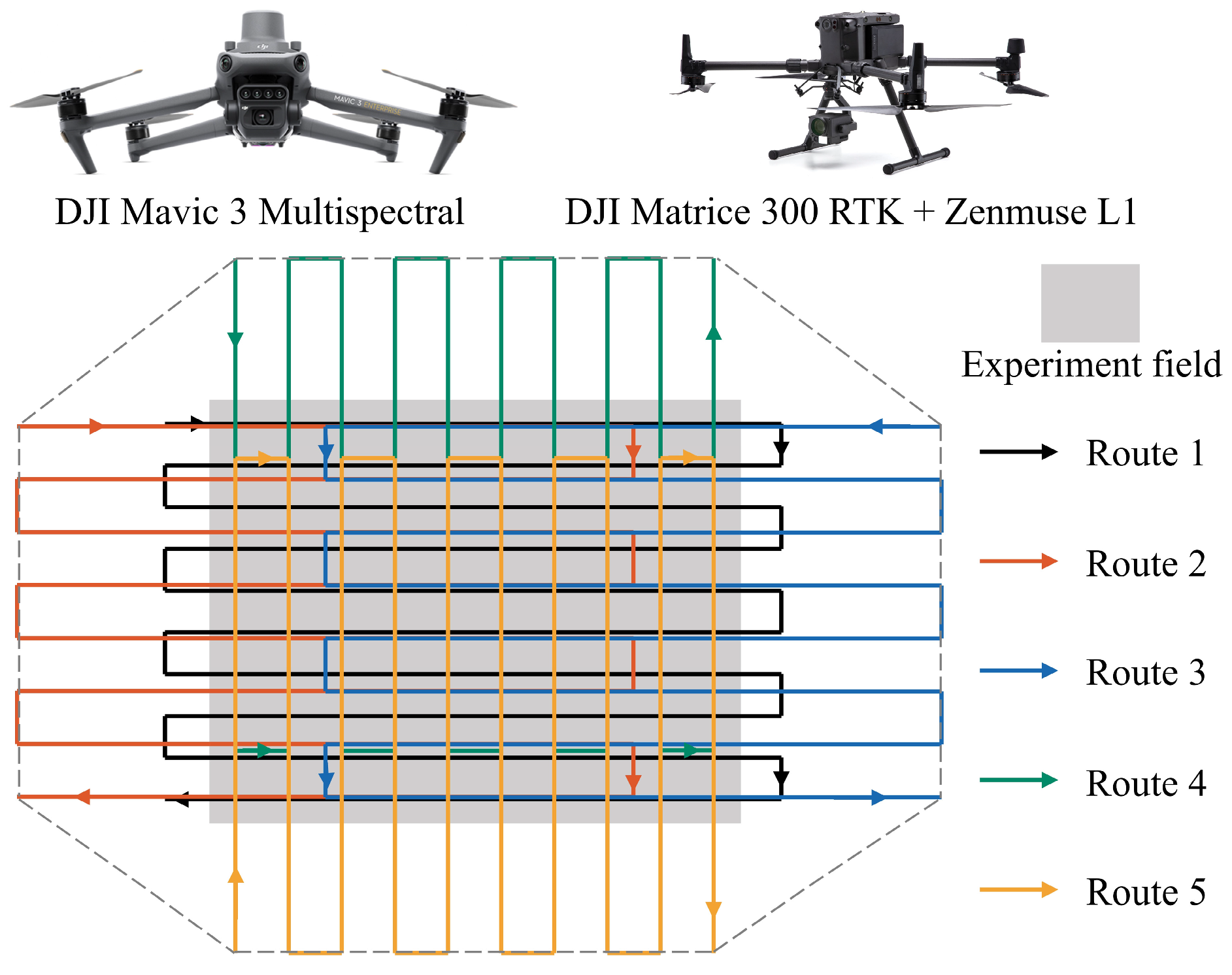
In this study, a DJI Mavic 3 Multispectral (M3M) (Da-Jiang Innovations Science and Technology Co., Ltd., Shenzhen, China) was used to capture MS imagery of the maize field at two growth stages: early silking (R1) and late dent (R5). The UAV was equipped with one RGB lens and four MS lenses (green: 560 ± 16 nm, red: 650 ± 16 nm, red edge: 730 ± 16 nm, near-infrared: 840 ± 26 nm). To minimize observational errors caused by cloud cover, the UAV flights were conducted under clear-sky and low-wind conditions. The imagery acquisition method was oblique photography, which can collect one orthophoto and oblique imagery in four different directions for making real 3D models (Figure 2). Data acquisition was performed from 11:00 a.m. to 1:00 p.m. at a flight altitude of 12 m, with forward and side overlaps maintained at 80% and 70%, respectively. Prior to the flight mission, three calibration boards with predetermined reflectivity values (25%, 50%, and 75%) were manually photographed for ensuing radiometric correction. The point clouds data were acquired using a DJI Matrice 300 RTK (Da-Jiang Innovations Science and Technology Co., Ltd., Shenzhen, China) equipped with a Zenmuse L1 laser sensor, which has a ranging accuracy of 3 cm at 100 m. The number of returns was set to 3, and the scan mode utilized a repetitive scanning pattern. However, the imagery acquisition method, including flight altitude and overlap ratios, was the same as for the M3M.

2.2.2. LAI Measurement and Processing

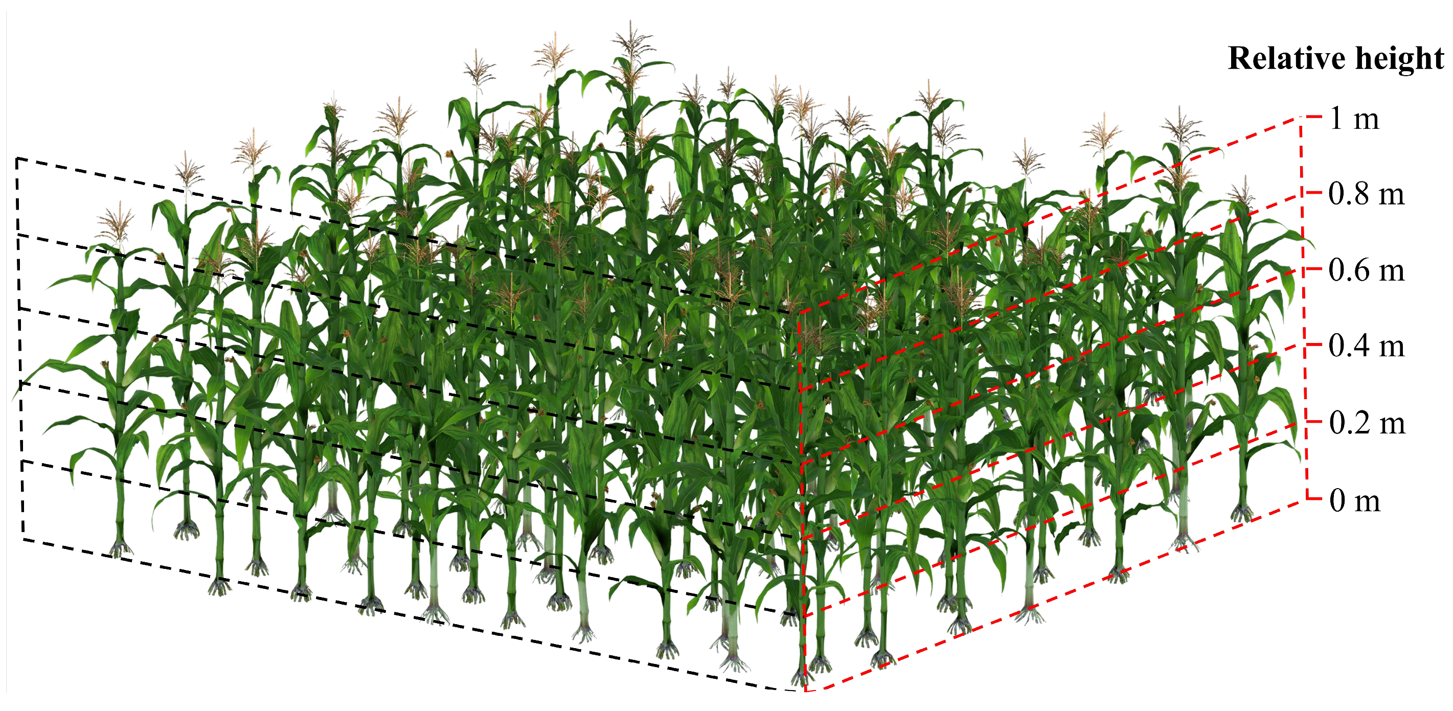
Field data measurements were performed after UAV imagery acquisition. Ten plants at the same growth stage were selected from each plot for height measurements. Then, these plants were divided into five layers based on their natural growth height in the field, and leaves from each layer were collected (Figure 3). To ensure sampling accuracy, the upper and lower boundaries of each layer were determined using a ruler and subsequently marked with a marker. Leaf area measurements were carried out using an LI-3000C (LI-COR Biosciences, Lincoln, OR, USA) system in conjunction with an LI-3050C transparent transmitter. Finally, the leaf area for each layer was determined, and the LAI of each plot was calculated based on planting density and land area.
One previous study showed that cumulative LAI values of maize exhibit an S-shaped upward trend with increasing relative height [21]. The vertical distribution patterns of maize canopy structures were explored by Yang et al. [22]. It was demonstrated that for various maize varieties entering the reproductive growth stage, the logistic equation most accurately fitted the relationship between canopy cumulative LAI values and relative height, with R2 values all exceeding 0.997. Subsequently, the vertical distribution function of LAD was derived using the differential method, and it was identified that the area with the densest leaf area (i.e., the maximum LAD) was located at a relative height of approximately 0.4 m. Other scholars have also demonstrated that changes in cumulative LAI values of maize canopies under different density treatments followed a logistic growth pattern [23]. To quantify the vertical distribution of canopy leaves, a “logistic” equation was used to fit the cumulative LAI values (Equation (1)). The coefficient of determination (R2) was used to evaluate the fit quality.
L A I H = M 1 + k e b H
Here, H refers to relative height, M refers to theoretical maximum LAI, L A I   H refers the sum of all leaf areas below height H, k refers to the initial value parameter, and b refers to the growth rate parameter, respectively.
Furthermore, the first derivative of the fitting curve was calculated to obtain the LAD distribution curve of the canopy (Equation (2)).
L A D H = d L A I H d H
Here, d refers to difference, H   refers to the height, and L A I H   refers to the LAI from the top of the canopy to a certain height H above.
The first derivative of the logistic curve exhibits a bell-shaped distribution that closely approximates the form of a normal distribution curve. In the context of normality testing, kurtosis and skewness are two principal statistical metrics that are commonly employed to evaluate whether a dataset conforms to a normal distribution. Therefore, the kurtosis and skewness of the LAD curve were extracted (Equations (3) and (4)). The greater the kurtosis, the denser the leaves were at a certain height within the canopy. Similarly, the greater the skewness, the closer the densest position of the leaves was to the lower layer.
K u r t o s i s = 1 n i = 1 n X i μ σ 4
S k e w n e s s = 1 n i = 1 n X i μ σ 3
Here, X i represents the LAD value, n is the number of samples, μ represents the average LAD, and σ represents the standard deviation of LAD.

2.2.3. Yield

Maize yield was obtained through destructive sampling at maturity. Twenty plants, including those with double ears and no ears, were consecutively sampled from each plot and manually threshed, dried, and weighed. The grain water content was determined by a grain water meter, and the grain weight was converted to 14.0% water content. Finally, the maize yield (t·ha−1) of each plot was calculated based on planting density and land area.

2.3. Imagery Processing

DJI Terra software (Version 4.5.0) was utilized to perform the MS reconstructions. Before carrying out the MS reconstruction, the calibrated board data were imported for radiometric correction, thereby enhancing the reliability of the final output. Following the reconstruction, four individual single-band maps were generated. To form the MS imagery from these four maps, the “build layer stack tool” in ENVI software (Version 5.6) was employed. A batch clipping process of the MS imagery was then performed using shapefiles that corresponded to each plot. These shapefiles were previously generated through the “create feature class tool” within ArcGIS software (Version 10.7). After rotation and clipping, the MS and RGB images exhibited a resolution of 331 × 331 pixels.
LiDAR point cloud data captured with the L1 sensor underwent reconstruction using DJI Terra software. The point cloud density was set to its maximum to ensure high-quality reconstruction, and point cloud accuracy optimization was enabled. The point cloud was then exported, followed by constructing a digital surface model (DSM) utilizing the elevation data derived from the point cloud.
Agisoft Metashape Professional software (Version 2.1.1) was used to process the RGB imagery captured by the M3M. The software employs structure from motion photogrammetry to generate a point cloud through the following steps: loading source data, aligning photos, camera calibration, and building the point cloud.
To enhance the fineness and density of the point clouds, LiDAR data were integrated with photogrammetry-derived point clouds. Geo-registration of these two datasets was achieved using real-time kinematic (RTK) positioning to establish ground control points (GCPs) within a unified coordinate system. This process was carried out using ContextCapture software (Version 10.20). The resulting fused point cloud enhanced the quality of the photogrammetric point cloud by leveraging the accuracy of the LiDAR dataset and improved the quality of the LiDAR point cloud by increasing its density with photogrammetric data. Finally, LiDAR360 software (Version 8.0) was utilized for point cloud denoising, filtering, and clipping.

2.4. Features Extraction

2.4.1. Vegetation Indices

Fifteen commonly used vegetation indices (VIs) were calculated from the four spectral bands of the MS imagery and used as predictors for estimating canopy indicators (Table 1).

2.4.2. Texture Indices

Eight commonly used texture indices (TIs) were calculated from the grayscale imagery of RGB imagery and used as predictors for estimating canopy indicators (Table 2).

2.5. Construction of Deep Learning Model

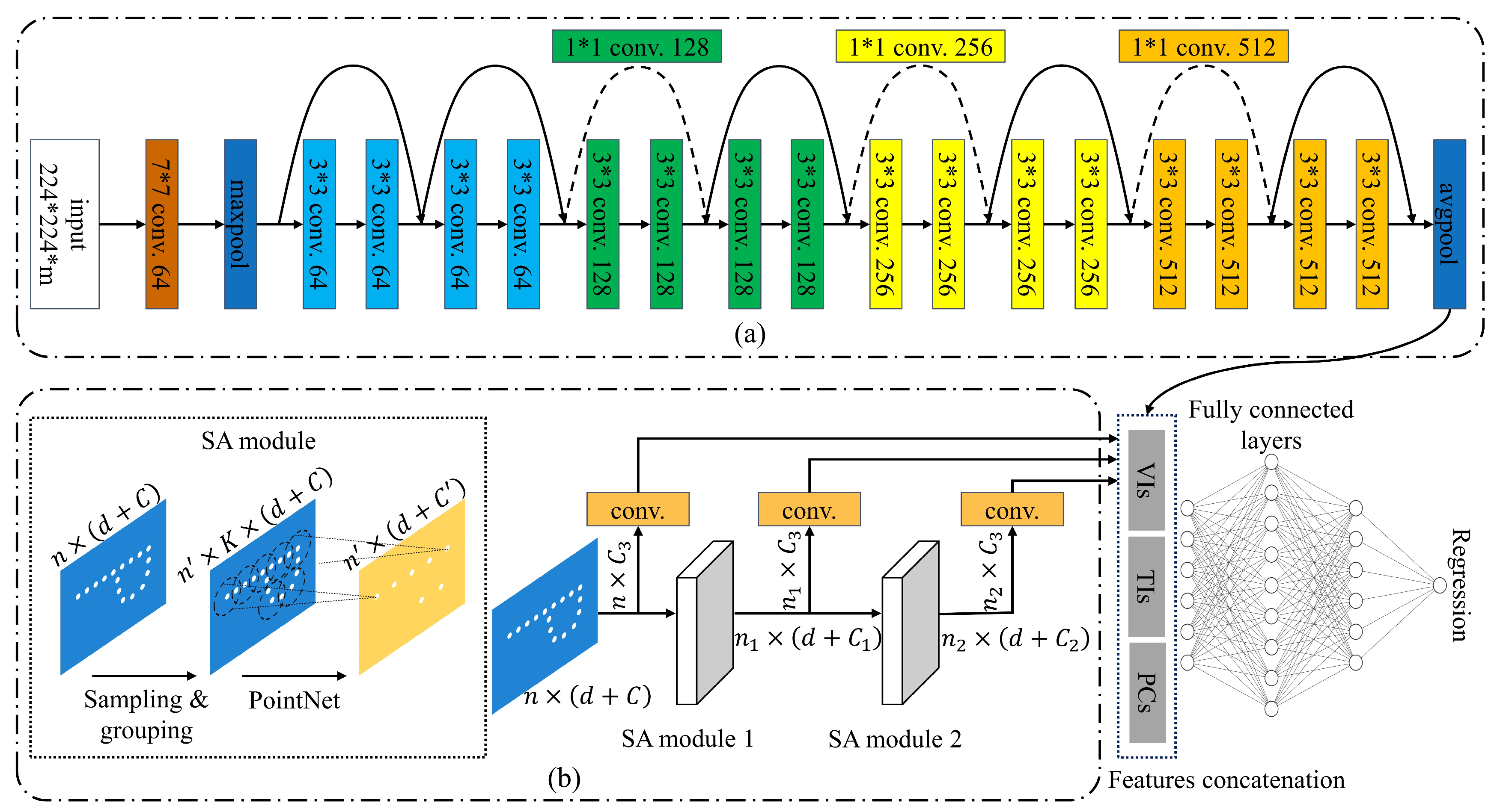
The VI and TI images were calculated using the MS and RGB images. Deep features were extracted from VI and TI images using an improved ResNet-18, while PointNet++ was employed for processing 3D point cloud data, to establish a deep network architecture for multi-source feature fusion (Figure 4). ResNet is a deep residual neural network designed to mitigate the degradation problem that arises with increasing network depth. Specifically, ResNet-18 comprises 18 layers organized into five distinct structural components (Figure 4a). Beginning with the conv2 layer, each subsequent layer contains two residual blocks, and each block is composed of two convolutional layers. PointNet is known as a deep neural network that is capable of directly processing raw, unordered, and unstructured point cloud data without requiring voxelization or projection-based preprocessing. PointNet++ is an enhanced version of PointNet that enhances the extraction of local features. It utilizes a hierarchical multi-layered architecture, wherein each layer extracts features across varying spatial scales (Figure 4b). Finally, the features derived from the two networks were subsequently fused using a concatenation approach and applied to the regression task of this study.
All analyses were performed on a workstation equipped with an Intel® CoreTM i9-12900K processor running at 3.2 GHz and two Nvidia RTX 2080Ti GPUs, each with 11 GB of VRAM. The software platform utilized was MATLAB 2024b. The fusion model was trained using the Adam optimizer with a learning rate of 0.001 and a batch size of 32. We trained the model for up to 100 epochs, employing early stopping with a patience of 10 epochs based on the validation loss to prevent overfitting. A validation split of 0.3 was used, stratified by site and planting density to maintain distributional consistency. The loss function was mean squared error, appropriate for our continuous prediction targets.

2.6. Model Accuracy Evaluation

To assess the model’s estimation performance, the R2, root-mean-square error (RMSE), and mean absolute error (MAE) were employed. The R2, RMSE, and MAE values were calculated as follows.
R 2 = 1 i = 1 N y i y i ^ 2 i = 1 N y i y i ¯ 2
R M S E = i = 1 N ( y i y i ^ ) 2 N
M A E = i = 1 N y i ^ y i N
Here, N is the number of samples, and y i and y i ^ are the measured and estimated indicator values, respectively, while   y i ¯ is the average measured indicator values.

3. Results

3.1. Descriptive Statistics

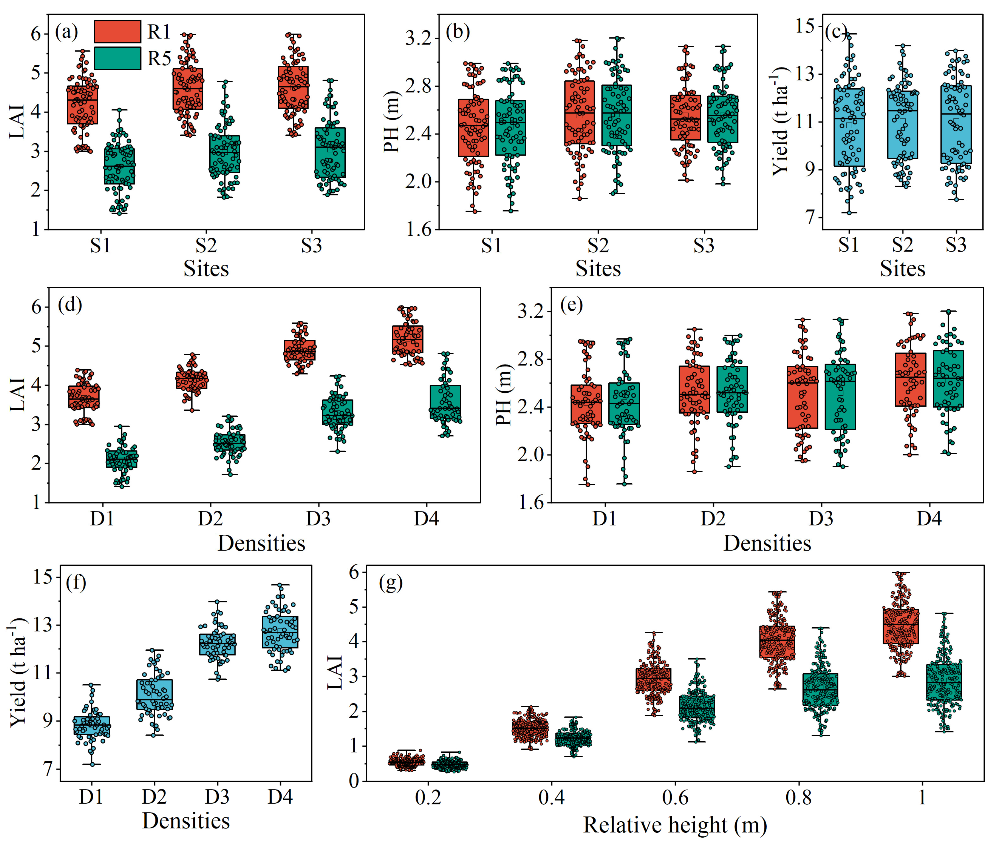
The LAI and PH were manually measured at the R1 and R5 growth stages, while yield was measured at maturity across three maize production regions. The results revealed significant differences in LAI between the R1 and R5 stages, while PH values remained relatively consistent (Figure 5a,b). At R1, LAI ranged from 3.001 to 5.988, with an average of 4.475, while at R5, it ranged from 1.414 to 4.810, with an average of 2.870. The PH across the study varied from 1.750 m to 3.201 m, with an average of 2.524 m. Yield ranged from 7.198 t·ha−1 to 14.679 t·ha−1, averaging 10.968 t·ha−1 (Figure 5c). Among the three regions, the LAI, PH, and yield in region S1 were lower than in regions S2 and S3, with no significant differences observed between S2 and S3. As planting density increased, both LAI and yield at R1 and R5 showed significant increases, while PH exhibited only a slight increase (Figure 5d–f). Additionally, with increasing relative height, the cumulative LAI values gradually increased (Figure 5g). The difference in cumulative LAI values between R1 and R5 was relatively small, 0.2 m and 0.4 m, but gradually increased, reaching a maximum difference of 2.174.

3.2. Construction of Canopy Architecture Indicators

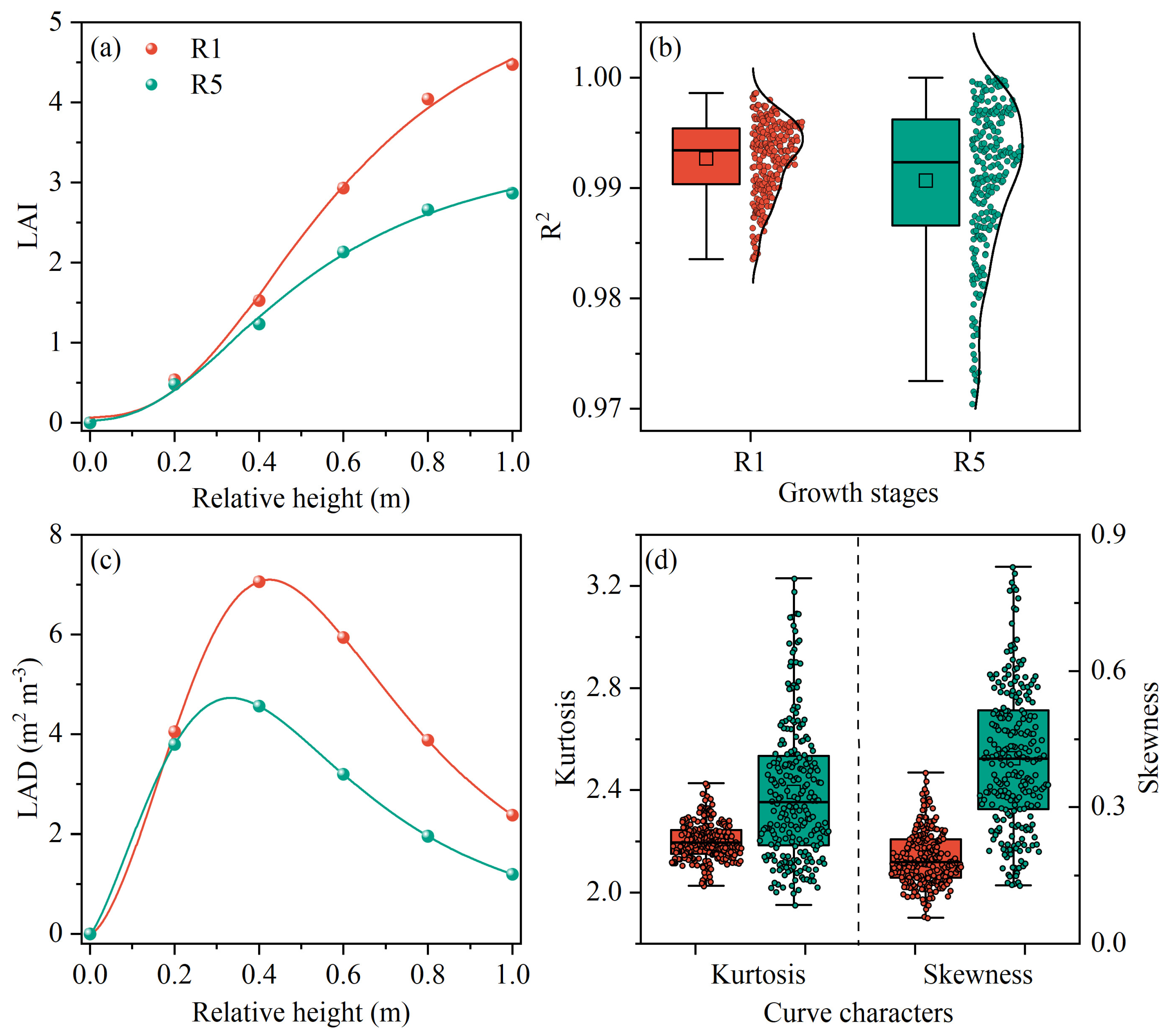
The results presented in Figure 6a illustrates the mean cumulative LAI values across different heights in all maize plots, with the initial LAI value set to zero. Figure 6b shows the distribution of the fitted R2 values, where R2 for R1 growth stage ranges from 0.984 to 0.999, with an average of 0.993, and R2 for R5 growth stage ranges from 0.970 to 0.992, with an average of 0.991, indicating an exceptionally high goodness of fit. After first-order differential of the fitted curves, the canopy LAD distribution curve was obtained, as depicted in Figure 6c. The peak represents the region of highest leaf area density within the canopy, which is observed near the lower two-fifths of the plant, closely aligning with actual conditions. The area under the LAD curve corresponds to the total LAI value, with larger areas indicating high LAI values. Finally, the kurtosis and skewness of the different LAD curves were calculated, with their distributions presented in Figure 6d. A higher kurtosis value is indicative of a greater leaf density at a specific height within the canopy. Similarly, a higher skewness value suggests that the peak leaf density is positioned lower within the canopy. The standard deviations for kurtosis and skewness at R1 was relatively small, 0.075 and 0.059, respectively, while those values at R5 were larger, 0.268 and 0.155, respectively.

3.3. Feasibility Analysis of Kurtosis and Skewness

3.3.1. Correlation Analysis

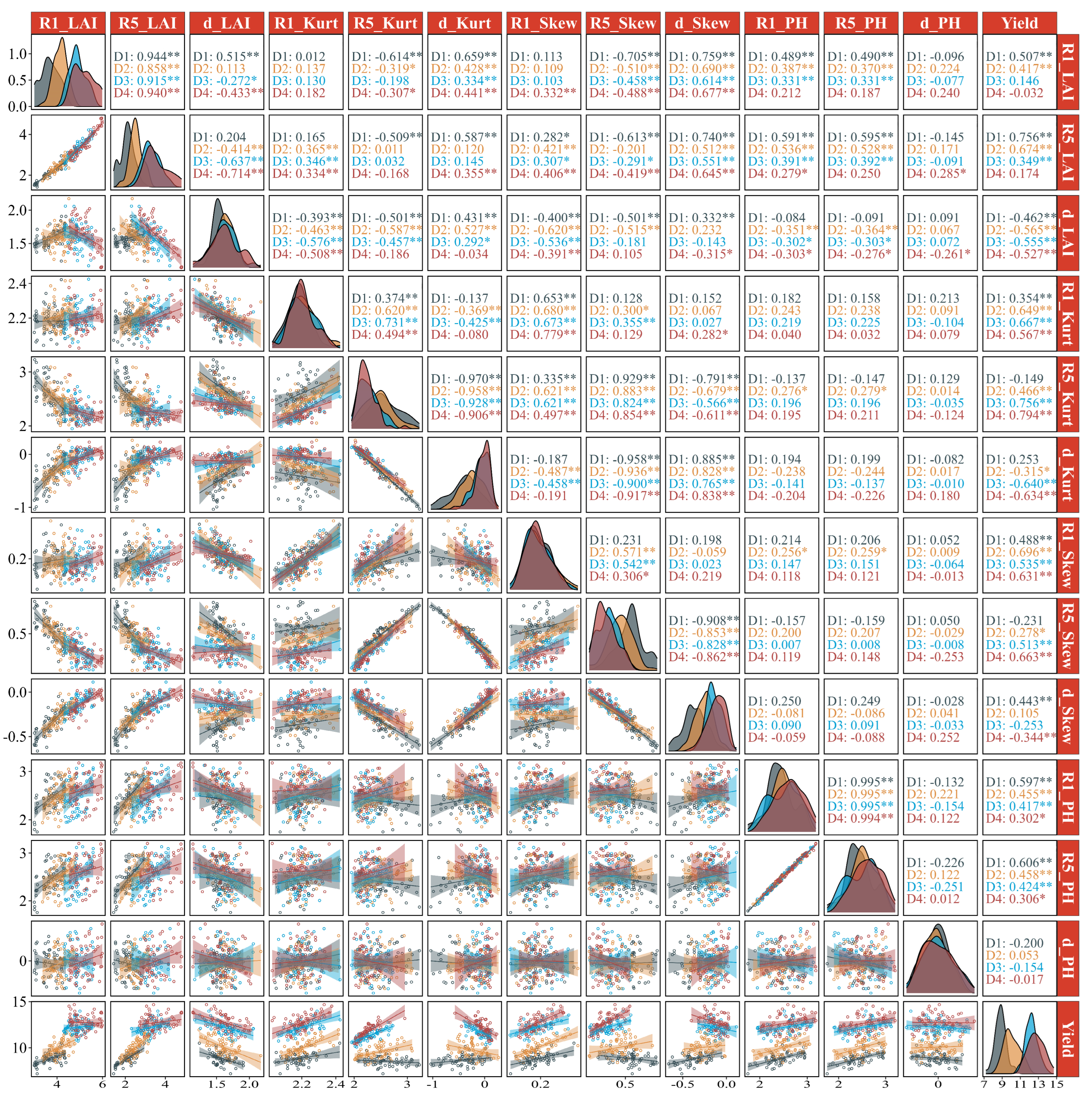
Pearson correlation analysis was conducted between manually measured LAI, kurtosis, skewness, PH, and the final yield (Figure 7). The results indicated that the LAI of R1 (R1_LAI) and R5 (R5_LAI) were significantly positively correlated with yield at D1 and D2 densities (p < 0.01), with a maximum correlation coefficient (r) of 0.756. As planting density increased, the correlation between R1_LAI, R5_LAI, and yield gradually decreased. Conversely, d_LAI was negatively correlated with yield across all four densities (p < 0.01), with a minimum r value of −0.462. Except at D1 density, the kurtosis of R1 (R1_kurtosis) and R5 (R5_kurtosis) were significantly positively correlated with yield (p < 0.01), with r values ranging from 0.466 to 0.794. In contrast, d_kurtosis was significantly negatively correlated with yield at D3 and D4 densities, while the correlation was weaker at D1 and D2 densities. The skewness of R1 was positively correlated with yield at all four densities (p < 0.01), whereas the skewness of R5 showed a positive correlation with yield only at D3 and D4 densities. Additionally, d_skewness was significantly correlated with yield at D1 and D4 densities (p < 0.01), with the correlation shifting from positive to negative as planting density increased. The PH of R1 (R1_PH) and R5 (R5_PH) was positively correlated with yield (p < 0.05), with a maximum r value of 0.606. However, as planting density increased, the correlation gradually decreased, with a minimum r value of 0.302. The correlation between d_PH and yield was not statistically significant, with a maximum r value of only −0.2.

3.3.2. Yield Estimation

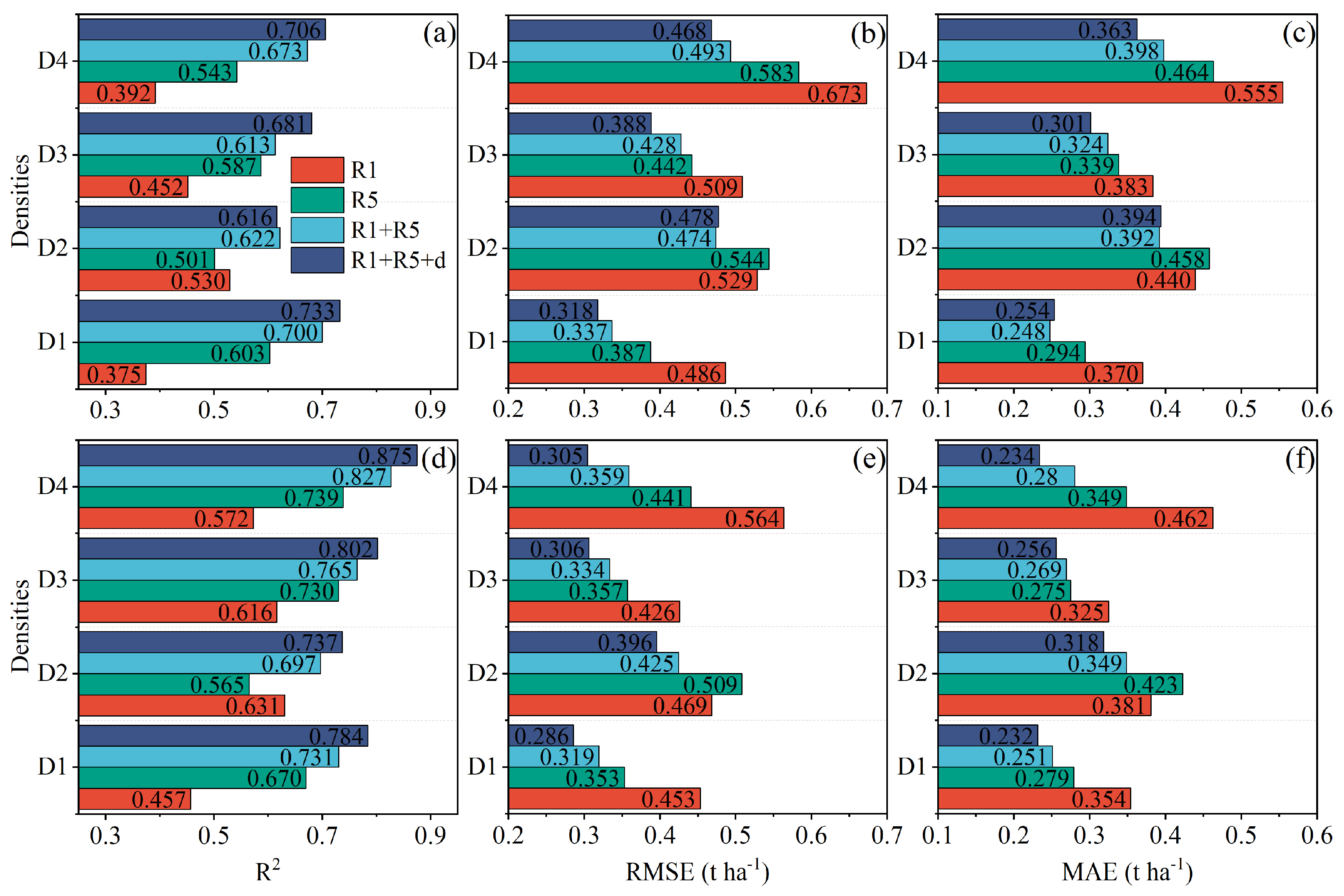
LAI and PH, which are key indicators of crop canopy structure, are strongly associated with photosynthetic efficiency, growth conditions, and yield. Therefore, these indicators have been widely used for yield estimation. In this study, yield estimation was conducted using measured LAI and PH, as well as their differences between the R1 and R5 growth stages (Figure 8a–c). When LAI and PH at the R1 stage were used alone for yield prediction, the models exhibited relatively low accuracy. Specifically, the R2 values for planting densities D1, D2, D3, and D4 were 0.375, 0.530, 0.452, and 0.392, respectively. Except at the D2 density, yield estimation accuracy at the R5 stage surpassed that of the R1 stage. Integrating data from both stages (R1 + R5) significantly improved yield estimation accuracy, with maximum increases in R2 of 0.325 and 0.130 compared to using only R1 or R5 data, respectively. Additionally, incorporating the differences in LAI and PH between the R1 and R5 stages (R1 + R5 + d) led to a further improvement in R2 values, except at the D2 density.
Furthermore, kurtosis and skewness, as well as their differences between the R1 and R5 growth stages, were incorporated into the yield estimation model (Figure 8d–f). At the four planting densities, significant improvements in R2 values were observed, ranging from 0.04 to 0.08, 0.06 to 0.13, 0.12 to 0.17, and 0.16 to 0.20, respectively. These results indicated that the predictive contribution of kurtosis and skewness increased progressively with higher planting density. When LAI, PH, kurtosis, and skewness, as well as their differences between the R1 and R5 growth stages, were integrated into the yield estimation model, accuracy reached its peak. The R2 values achieved were 0.784, 0.737, 0.802, and 0.875 for the respective planting densities.

3.4. Canopy Indicator Estimation

3.4.1. Correlation Between VIs and Kurtosis and Skewness

The correlations between various VIs and kurtosis and skewness are presented in Table 3. In general, correlations at the R1 stage were lower than those at the R5 stage. Significant correlations (p < 0.05) between kurtosis and all VIs were observed at both the R1 and R5 growth stages, except for Cig, Datt, and PSRI. OSAVI and GDVI showed the strongest correlations with kurtosis, with r values of 0.481 and 0.579 at the R1 and R5 stages, respectively. Regarding skewness, significant correlations (p < 0.05) were detected for all VIs except GNDVI and PSRI. Cig and MCARI demonstrated the highest correlations with skewness during the R1 and R5 stages, with corresponding r values of 0.461 and 0.562, respectively.
For TIs, significant correlations (p < 0.05) with kurtosis were observed at both the R1 and R5 growth stages, except for the mean and second moment. Correlation and contrast showed the strongest correlations with kurtosis during the R1 and R5 stages, with r values of 0.385 and 0.453, respectively. Regarding skewness, significant correlations (p < 0.05) were detected for all TIs except mean, dissimilarity, and second moment. Entropy and contrast exhibited the strongest correlations with skewness during the R1 and R5 stages, with r values of 0.370 and 0.417, respectively. Notably, the correlations between TIs and kurtosis and skewness were generally lower than those observed for VIs. In summary, VIs provided more reliable associations with both kurtosis and skewness than TIs, especially in later growth stages, suggesting their greater utility for capturing distributional traits of canopy.

3.4.2. Kurtosis and Skewness Estimation Results

To estimate kurtosis and skewness, deep learning models were developed using three types of input data: VI images, TI images, and point clouds. The results are presented in Table 4. Among the three data types, point cloud data yielded the highest estimation accuracy, with R2 values exceeding 0.69 for both kurtosis and skewness. In contrast, models based on VI images achieved lower performance, with R2 values ranging from 0.43 to 0.56. TI image-based models demonstrated the lowest predictive accuracy, with R2 values not surpassing 0.45. Upon integrating all three data sources, a significant improvement in model performance was observed. Specifically, during the R1 and R5 growth stages, the R2 values for kurtosis estimation increased to 0.792 and 0.841, respectively, while those for skewness estimation reached 0.815 and 0.859. These results indicate that multi-modal data fusion can significantly enhance the predictive capacity of deep learning models for canopy structural indicators.

4. Discussion

4.1. Vertical Distribution of Leaf Area in Maize Canopy

The vertical distribution of leaf area in the maize canopy is of great theoretical and practical importance. Understanding how light is intercepted at different canopy layers can help improve photosynthetic efficiency and inform decisions on planting density, irrigation and fertilization strategies, and lodging resistance cultivation. Ultimately, these measures contribute to better use of light and heat resources and support higher crop productivity. Zhao et al. [39] demonstrated significant differences in the vertical distribution characteristics of canopy leaf area under different planting densities. Non-destructive stratified measurements were performed by Hirooka et al. [40] using an LAI-2200 plant canopy analyzer. The results showed that the parameters calculated from the statistical moment equations were more stable for evaluating the cultivar characteristics or the effect of the treatments. This is inconsistent with the results of this study. This may be because this study used destructive sampling, while their study used LAI-2200. The LAI-2200 has a viewing angle of 148° and a lens thickness of 3 cm, which could not evaluate just above the measurement point. In addition, their study also showed that the measurement error between LAI-2200 and destructive sampling was 21.6%. Leaf angle serves as an indicator that defines the angle between the leaf blade and the stem, representing a typical individual phenotype. The various leaf positions exhibit distinct pinch angles, which complicates the precise characterization of the vertical distribution of canopy leaves. LAD uniformity is employed to assess the consistency of LAD in the vertical direction, which can be quantified using the standard deviation and coefficient of variation, yet it fails to precisely capture the specific distribution of LAD. Our study introduced kurtosis and skewness indicators, which offer a novel perspective for the quantitative analysis of the vertical distribution of the maize canopy leaf area and provide a high-throughput estimation method with practicality.

4.2. Effect of Canopy Architecture Indicators on Photosynthesis and Yield

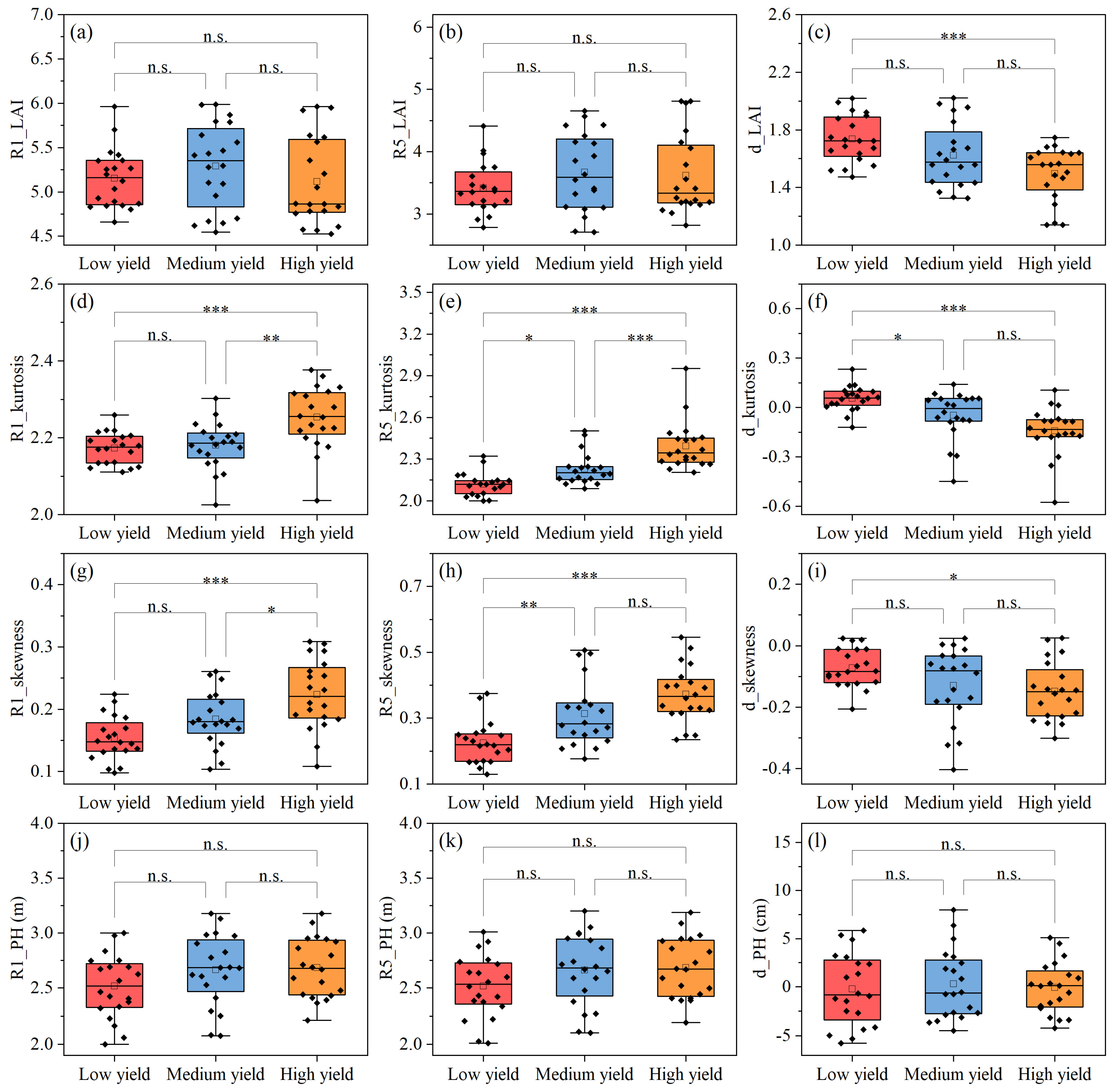
In the current study, the varieties under different densities were classified into three categories based on their yields: low yield, medium yield, and high yield. The canopy indicators for each yield level under the D4 density are presented in Figure 9. The results indicated that there were no significant differences in LAI across the different yield levels. The average LAI values for the low-yield, medium-yield, and high-yield maize groups during the R1 stage were 5.153, 5.292, and 5.114, respectively, while the average values during the R5 stage were 3.417, 3.668, and 3.619, respectively (Figure 9a,b). The differences between the R1 and R5 stages were highly significant (p < 0.001) in both low-yield and high-yield maize (Figure 9c), indicating that high-yield maize varieties exhibit stronger green retention and are capable of producing more photosynthetic products. Zhang et al. [41] also demonstrated that during the grain filling stage, varieties with long photosynthesis time and strong stay-green ability achieve high yields, making these traits ideal for breeding selection. However, Li et al. [42] showed that high-density planting of maize can cause premature leaf senescence, which leads to a reduction in lower leaves and decreased root function, ultimately reducing yield. This presents a challenge in high-density planting and breeding of ideal architecture.
A larger kurtosis indicates a high density of leaves at a certain height, which may hinder the photosynthesis of the lower leaves. Conversely, a small kurtosis may reduce the projected area, suggesting a lower LAI. A larger skewness indicates that the maximum LAD occurs closer to the soil, suggesting that the upper and middle leaves receive more light, while the lower leaves act as a safety net, minimizing sunlight wastage. Therefore, a combination of larger kurtosis and skewness indicates high yield potential and serves as an important quantitative indicator of the ideal maize architecture. In this study, the kurtosis and skewness of the high-yield group were significantly higher than those of the low-yield group (p < 0.001) (Figure 9d–i), which is consistent with anticipated patterns. However, in a superhigh-yield maize population, the planting density exceeded 105 plants ha−1 and the LAI surpassed 8 [5], whereas in this study, the maximum LAI did not exceed 6. Therefore, planting density will be increased further in future studies to validate the effectiveness of the kurtosis and skewness indicators.
The PH level significantly influences the light interception capacity and light energy utilization efficiency within the maize canopy. Generally, a higher PH facilitates increased yields [43]. There was a significant positive correlation between yield and PH at lower planting densities (p < 0.01) (Figure 7). However, this correlation became non-significant at high planting densities (p > 0.05) (Figure 9j–l). Shapiro et al. [44] showed that PH generally increases with increasing planting density, but when it exceeds the optimal density, PH decreases. As planting density increased, both PH and ear height increased, while stem diameter gradually became thinner. This led to a decrease in lodging resistance and an increase in the empty stalk rate, ultimately affecting maize yield [45].

4.3. Effect of Planting Density on Photosynthesis and the Estimation Accuracy of Canopy Indicators

Approximately 35–40% of the increase in maize production in China is attributed to genetic improvement, while 60–65% is achieved through management practices [46]. Niu et al. [47] demonstrated that increasing planting density is an effective strategy for enhancing maize yield. The effect of planting density on maize photosynthesis is primarily reflected in light capture efficiency, the distribution of photosynthetic products, and microclimate changes within the population. High-density planting increases leaf overlap and shading, and an excessively high LAI results in insufficient light reaching the lower leaves, thereby reducing photosynthetic efficiency. Additionally, under high-density conditions, the allocation of photosynthetic products to roots and stems increases, while allocation to leaves and fruits decreases, potentially negatively impacting the final yield and quality of crops [48]. Finally, high-density planting typically increases humidity and temperature in the field. While increased humidity can help slow plant transpiration, excessive humidity and temperature may promote disease occurrence and negatively affect photosynthesis [45]. While low-density planting allows maize to receive more light, the overall light utilization rate remains low [49]. Low-density planting also reduces competition among plants, enabling each plant to obtain more resources, thereby enhancing photosynthetic efficiency and the accumulation of photosynthetic products. However, excessively low planting density may lead to underutilization of land and light resources, thereby reducing overall production benefits. In summary, planting density is a crucial cultivation measure for balancing resource allocation between crop population and individual plants, establishing a reasonable canopy architecture, and maintaining high photosynthetic performance and requires future attention.
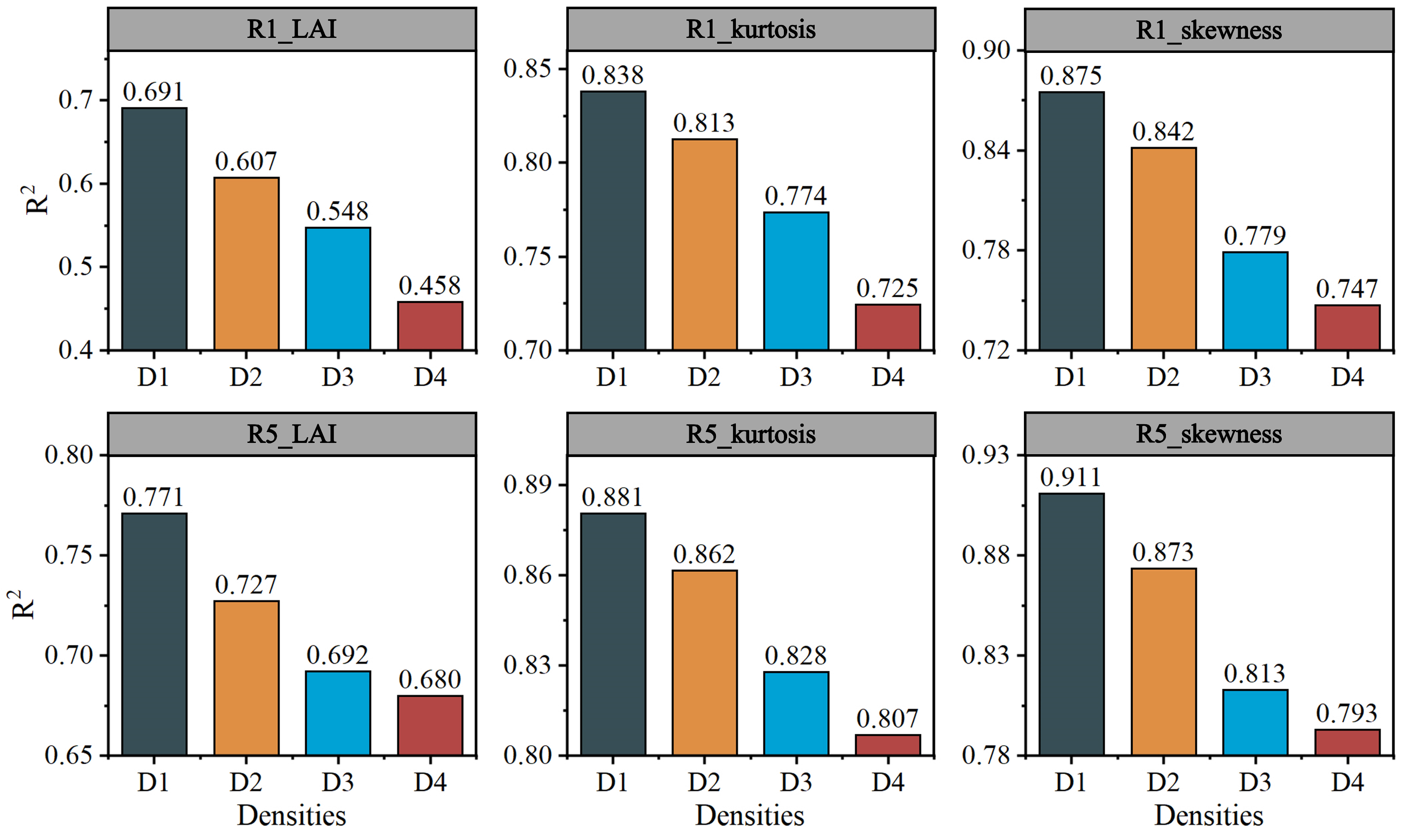
Accurate estimation of canopy indicators is crucial for effective crop management and yield prediction. However, variations in planting density significantly impact the accuracy of canopy indicator estimation. Figure 10 illustrates that as planting density increases, the estimated R2 values of LAI, kurtosis, and skewness gradually decrease. The R2 value of R1_LAI shows the most significant decrease, dropping by 0.233, whereas R5_kurtosis exhibits the smallest decrease, with a value of 0.074. The R2 values of LAI, kurtosis, and skewness decreased by 0.162, 0.104, and 0.123, respectively, indicating that the estimation accuracy of LAI is most affected by changes in planting density, whereas the accuracy of kurtosis estimation is least affected. From a modeling perspective, higher-density scenarios reduced the signal-to-noise ratio in both multispectral reflectance (due to shadowing and mixed pixels) and LiDAR returns (due to occluded lower layers), which partly explains the R2 decline. The LAI, kurtosis, and skewness were all related to the internal architecture of the canopy and were influenced by canopy density.

5. Conclusions

The current study primarily focused on estimation of maize yield through introducing two novel canopy indicators (kurtosis and skewness) that describe maize architecture based on the vertical distribution of leaves. Correlation analysis between these indicators and yield revealed significant relationships at the R1 and R5 growth stages, with maximum r of 0.696 and 0.794, respectively. Yield was estimated by combining LAI, kurtosis, skewness, and PH, resulting in R2 values of 0.792, 0.779, 0.796, and 0.865 at D1, D2, D3, and D4 planting densities, respectively.
The estimation of LAI, kurtosis, skewness, and PH using a fusion of UAV multispectral data, LiDAR point clouds, and oblique photography point clouds demonstrated high accuracy across various sites, plant densities, cultivars, and growth stages, with R2 values ranging from 0.79 to 0.93. Maize yield was also estimated using the four estimated canopy indicators, resulting in R2 values of 0.636, 0.688, 0.716, and 0.775 for D1, D2, D3, and D4 planting densities, respectively. The study further demonstrated that yield estimation based on canopy indicators was more accurate than direct yield estimation from UAV-derived parameters. Given these findings, the combination of these four indicators is not only promising for maize yield assessment but also valuable for screening ideal canopy architecture in breeding programs. Since maize is a tall crop, future research should explore the applicability of the proposed canopy indicators to other crops or field conditions.

Author Contributions

Conceptualization, S.Z., D.H., T.Y., T.L. and C.S.; data curation, D.H.; formal analysis, W.Z.; funding acquisition, T.L. and C.S.; investigation, T.Y. and Z.Y.; methodology, S.Z., D.H., W.Z., Z.Y. and C.S.; project administration, T.L. and C.S.; resources, T.L.; software, S.Z. and D.H.; supervision, Z.Y.; validation, S.Z., W.Z. and C.S.; visualization, S.Z. and T.Y.; writing—original draft, S.Z.; writing—review & editing, S.Z. All authors have read and agreed to the published version of the manuscript.

Funding

This research was funded by the Key Research and Development Program (Modern Agriculture) of Jiangsu Province (BE2022335, BE2022338, BE2022342-2), National Key Research and Development Program of China (2023YFD1202200), National Natural Science Foundation of China (32172110), Priority Academic Program Development of Jiangsu Higher Education Institutions (PAPD), and Biological Breeding Zhongshan Laboratory Program of Jiangsu Province (ZSBBL-KY2023-05).

Data Availability Statement

The original data presented in the study are included in the article. Further inquiries can be directed to the corresponding author.

Conflicts of Interest

The authors declare no conflicts of interest.

Abbreviations

CCCanopy coverage
LAILeaf area index
PHPlant height
LADLeaf area density
MSMultispectral
LiDARLight detection and ranging
UAVUnmanned aerial vehicle
M3MMavic 3 multispectral
R1Silking stage
R5Dent stage
R2Coefficient of determination
VIsVegetation indices
TIsTexture indices
GLCMGray-level co-occurrence matrix
RMSERoot-mean-square error
MAEMean absolute error

References

  1. Feng, L.Y.; Raza, M.A.; Shi, J.Y.; Ansar, M.; Titriku, J.K.; Meraj, T.A.; Shah, G.A.; Ahmed, Z.; Saleem, A.; Liu, W.G.; et al. Delayed maize leaf senescence increases the land equivalent ratio of maize soybean relay intercropping system. Eur. J. Agron. 2020, 118, 126092. [Google Scholar] [CrossRef]
  2. Luo, N.; Meng, Q.; Feng, P.; Qu, Z.; Yu, Y.; Liu, D.L.; Müller, C.; Wang, P. China can be self-sufficient in maize production by 2030 with optimal crop management. Nat. Commun. 2023, 14, 2637. [Google Scholar] [CrossRef]
  3. Shafi, M.; Bakht, J.; Ali, S.; Khan, H.; Khan, M.A.; Sharif, M. Effect of planting density on phenology, growth and yield of maize (Zea mays L.). Pak. J. Bot. 2012, 44, 691–696. [Google Scholar]
  4. Li, R.F.; Zhang, G.Q.; Liu, G.Z.; Wang, K.R.; Xie, R.Z.; Hou, P.; Ming, B.; Wang, Z.G.; Li, S.K. Improving the yield potential in maize by constructing the ideal plant type and optimizing the maize canopy structure. Food Energy Secur. 2021, 10, e312. [Google Scholar] [CrossRef]
  5. Tian, J.G.; Wang, C.L.; Chen, F.Y.; Qin, W.C.; Yang, H.; Zhao, S.H.; Xia, J.L.; Du, X.; Zhu, Y.F.; Wu, L.S.; et al. Maize smart-canopy architecture enhances yield at high densities. Nature 2024, 632, 576–584. [Google Scholar] [CrossRef]
  6. Castro-Valdecantos, P.; Apolo-Apolo, O.E.; Pérez-Ruiz, M.; Egea, G. Leaf area index estimations by deep learning models using RGB images and data fusion in maize. Precis. Agric. 2022, 23, 1949–1966. [Google Scholar] [CrossRef]
  7. Gano, B.; Dembele, J.S.B.; Ndour, A.; Luquet, D.; Beurier, G.; Diouf, D.; Audebert, A. Using UAV borne, multi-spectral imaging for the field phenotyping of shoot biomass, leaf area index and height of West African sorghum varieties under two contrasted water conditions. Agronomy 2021, 11, 850. [Google Scholar] [CrossRef]
  8. Wang, Z.K.; Zhao, X.N.; Wu, P.T.; He, J.Q.; Chen, X.L.; Gao, Y.; Cao, X.C. Radiation interception and utilization by wheat/maize strip intercropping systems. Agric. For. Meteorol. 2015, 204, 58–66. [Google Scholar] [CrossRef]
  9. Fischer, K.S.; Edmeades, G.O.; Johnson, E.C. Recurrent selection for reduced tassel branch number and reduced leaf area density above the ear in tropical maize populations1. Crop Sci. 1987, 27, 1150–1156. [Google Scholar] [CrossRef]
  10. Ross, J.; Ross, V.; Koppel, A. Estimation of leaf area and its vertical distribution during growth period. Agric. For. Meteorol. 2000, 101, 237–246. [Google Scholar] [CrossRef]
  11. Chatterjee, S.; Baath, G.S.; Sapkota, B.R.; Flynn, K.C.; Smith, D.R. Enhancing LAI estimation using multispectral imagery and machine learning: A comparison between reflectance-based and vegetation indices-based approaches. Comput. Electron. Agric. 2025, 230, 109790. [Google Scholar] [CrossRef]
  12. Nguy-Robertson, A.L.; Peng, Y.; Gitelson, A.A.; Arkebauer, T.J.; Pimstein, A.; Herrmann, I.; Karnieli, A.; Rundquist, D.C.; Bonfil, D.J. Estimating green LAI in four crops: Potential of determining optimal spectral bands for a universal algorithm. Agric. For. Meteorol. 2014, 192, 140–148. [Google Scholar] [CrossRef]
  13. Zhao, D.; Yang, G.; Xu, T.; Yu, F.; Zhang, C.; Cheng, Z.; Ren, L.; Yang, H. Dynamic maize true leaf area index retrieval with KGCNN and TL and integrated 3D radiative transfer modeling for crop phenotyping. Plant Phenomics 2025, 7, 100004. [Google Scholar] [CrossRef]
  14. Savinelli, B.; Tagliabue, G.; Vignali, L.; Garzonio, R.; Gentili, R.; Panigada, C.; Rossini, M. Integrating drone-based LiDAR and multispectral data for tree monitoring. Drones 2024, 8, 744. [Google Scholar] [CrossRef]
  15. Nguyen, C.; Sagan, V.; Bhadra, S.; Moose, S. UAV multisensory data fusion and multi-task deep learning for high-throughput maize phenotyping. Sensors 2023, 23, 1827. [Google Scholar] [CrossRef]
  16. Wang, H.; Zhang, W.; Yang, G.; Lei, L.; Han, S.; Xu, W.; Chen, R.; Zhang, C.; Yang, H. Maize ear height and ear–plant height ratio estimation with LiDAR data and vertical leaf area profile. Remote Sens. 2023, 15, 964. [Google Scholar] [CrossRef]
  17. Lei, L.; Qiu, C.X.; Li, Z.H.; Han, D.; Han, L.; Zhu, Y.H.; Wu, J.T.; Xu, B.; Feng, H.K.; Yang, H.; et al. Effect of leaf occlusion on leaf area index inversion of maize using UAV-LiDAR data. Remote Sens. 2019, 11, 1067. [Google Scholar] [CrossRef]
  18. Khun, K.; Tremblay, N.; Panneton, B.; Vigneault, P.; Lord, E.; Cavayas, F.; Codjia, C. Use of oblique RGB imagery and apparent surface area of plants for early estimation of above-ground corn biomass. Remote Sens. 2021, 13, 4032. [Google Scholar] [CrossRef]
  19. Che, Y.P.; Wang, Q.; Xie, Z.W.; Zhou, L.; Li, S.W.; Hui, F.; Wang, X.Q.; Li, B.G.; Ma, Y.T. Estimation of maize plant height and leaf area index dynamics using an unmanned aerial vehicle with oblique and nadir photography. Ann. Bot. 2020, 126, 765–773. [Google Scholar] [CrossRef]
  20. Wang, Y.; Wen, W.; Wu, S.; Wang, C.; Yu, Z.; Guo, X.; Zhao, C. Maize plant phenotyping: Comparing 3D laser scanning, multi-view stereo reconstruction, and 3D digitizing estimates. Remote Sens. 2018, 11, 63. [Google Scholar] [CrossRef]
  21. Liu, S.B.; Jin, X.L.; Nie, C.W.; Wang, S.Y.; Yu, X.; Cheng, M.H.; Shao, M.C.; Wang, Z.X.; Tuohuti, N.; Bai, Y.; et al. Estimating leaf area index using unmanned aerial vehicle data: Shallow vs. deep machine learning algorithms. Plant Physiol. 2021, 187, 1551–1576. [Google Scholar] [CrossRef]
  22. Yang, J.; Lu, Q. A study on mathematical models of canopy architecture for maize population. J. Shanxi Agric. Univ. 1996, 16, 347–349. [Google Scholar]
  23. Hirooka, Y.; Homma, K.; Shiraiwa, T.; Kuwada, M. Parameterization of leaf growth in rice (Oryza sativa L.) utilizing a plant canopy analyzer. Field Crops Res. 2016, 186, 117–123. [Google Scholar] [CrossRef]
  24. Main, R.; Cho, M.A.; Mathieu, R.; O’kennedy, M.M.; Ramoelo, A.; Koch, S. An investigation into robust spectral indices for leaf chlorophyll estimation. ISPRS J. Photogramm. Remote Sens. 2011, 66, 751–761. [Google Scholar] [CrossRef]
  25. Ahamed, T.; Tian, L.; Zhang, Y.; Ting, K.C. A review of remote sensing methods for biomass feedstock production. Biomass Bioenerg. 2011, 35, 2455–2469. [Google Scholar] [CrossRef]
  26. Datt, B. Remote sensing of water content in eucalyptus leaves. Aust. J. Bot. 1999, 47, 909–923. [Google Scholar] [CrossRef]
  27. Zhu, Y.; Yao, X.; Tian, Y.C.; Liu, X.J.; Cao, W.X. Analysis of common canopy vegetation indices for indicating leaf nitrogen accumulations in wheat and rice. Int. J. Appl. Earth Obs. 2008, 10, 1–10. [Google Scholar] [CrossRef]
  28. Tucker, C.J.; Elgin, J.H.; Iii, M.M.; Fan, C.J. Monitoring corn and soybean crop development with hand-held radiometer spectral data. Remote Sens. Environ. 1979, 8, 237–248. [Google Scholar] [CrossRef]
  29. Haboudane, D.; Miller, J.R.; Pattey, E.; Zarco-Tejada, P.J.; Strachan, I.B. Hyperspectral vegetation indices and novel algorithms for predicting green LAI of crop canopies: Modeling and validation in the context of precision agriculture. Remote Sens. Environ. 2004, 90, 337–352. [Google Scholar] [CrossRef]
  30. Rouse, J.W., Jr.; Haas, R.H.; Schell, J.; Deering, D. Monitoring the Vernal Advancement and Retrogradation (Green Wave Effect) of Natural Vegetation; National Aeronautics and Space Administration: Washington, DC, USA, 1973. [Google Scholar]
  31. Yang, C.; Everitt, J.H.; Bradford, J.M.; Murden, D. Airborne hyperspectral imagery and yield monitor data for mapping cotton yield variability. Precis. Agric. 2004, 5, 445–461. [Google Scholar] [CrossRef]
  32. Tian, Y.C.; Yao, X.; Yang, J.; Cao, W.X.; Hannaway, D.B.; Zhu, Y. Assessing newly developed and published vegetation indices for estimating rice leaf nitrogen concentration with ground- and space-based hyperspectral reflectance. Field Crops Res. 2011, 120, 299–310. [Google Scholar] [CrossRef]
  33. Daughtry, C.S.T.; Walthall, C.L.; Kim, M.S.; De Colstoun, E.B.; Mcmurtrey, J.E. Estimating corn leaf chlorophyll concentration from leaf and canopy reflectance. Remote Sens. Environ. 2000, 74, 229–239. [Google Scholar] [CrossRef]
  34. Merzlyak, M.N.; Gitelson, A.A.; Chivkunova, O.B.; Rakitin, V.Y. Non-destructive optical detection of pigment changes during leaf senescence and fruit ripening. Physiol. Plant. 1999, 106, 135–141. [Google Scholar] [CrossRef]
  35. Broge, N.H.; Mortensen, J.V. Deriving green crop area index and canopy chlorophyll density of winter wheat from spectral reflectance data. Remote Sens. Environ. 2002, 81, 45–57. [Google Scholar] [CrossRef]
  36. Haboudane, D.; Miller, J.R.; Tremblay, N.; Zarco-Tejada, P.J.; Dextraze, L. Integrated narrow-band vegetation indices for prediction of crop chlorophyll content for application to precision agriculture. Remote Sens. Environ. 2002, 81, 416–426. [Google Scholar] [CrossRef]
  37. Hall-Beyer, M. Practical guidelines for choosing GLCM textures to use in landscape classification tasks over a range of moderate spatial scales. Int. J. Remote Sens. 2017, 38, 1312–1338. [Google Scholar] [CrossRef]
  38. Rodriguez-Galiano, V.F.; Chica-Olmo, M.; Abarca-Hernandez, F.; Atkinson, P.M.; Jeganathan, C. Random forest classification of mediterranean land cover using multi-seasonal imagery and multi-seasonal texture. Remote Sens. Environ. 2012, 121, 93–107. [Google Scholar] [CrossRef]
  39. Zhao, K.; Xu, X.; Yuan, Y.; Zhang, H. Population structure and light distribution in maize fields. Acta Agron. Sin. 1963, 2, 321–332. [Google Scholar]
  40. Hirooka, Y.; Homma, K.; Shiraiwa, T. Parameterization of the vertical distribution of leaf area index (LAI) in rice (Oryza sativa L.) using a plant canopy analyzer. Sci. Rep. 2018, 8, 6387. [Google Scholar] [CrossRef] [PubMed]
  41. Zhang, J.; Fengler, K.A.; Van Hemert, J.L.; Gupta, R.; Mongar, N.; Sun, J.D.; Allen, W.B.; Wang, Y.; Weers, B.; Mo, H.; et al. Identification and characterization of a novel stay-green QTL that increases yield in maize. Plant Biotechnol. J. 2019, 17, 2272–2285. [Google Scholar] [CrossRef]
  42. Li, R.F.; Hu, D.D.; Ren, H.; Yang, Q.L.; Dong, S.T.; Zhang, J.W.; Zhao, B.; Liu, P. How delaying post-silking senescence in lower leaves of maize plants increases carbon and nitrogen accumulation and grain yield. Crop J. 2022, 10, 853–863. [Google Scholar] [CrossRef]
  43. Liu, N.; Li, L.; Li, H.T.; Liu, Z.M.; Lu, Y.; Shao, L.W. Selecting maize cultivars to regulate canopy structure and light interception for high yield. Agron. J. 2023, 115, 770–780. [Google Scholar] [CrossRef]
  44. Shapiro, C.A.; Wortmann, C.S. Corn response to nitrogen rate, row spacing, and plant density in eastern Nebraska. Agron. J. 2006, 98, 529–535. [Google Scholar] [CrossRef]
  45. Jafari, F.; Wang, B.B.; Wang, H.Y.; Zou, J.J. Breeding maize of ideal plant architecture for high-density planting tolerance through modulating shade avoidance response and beyond. J. Integr. Plant Biol. 2024, 66, 849–864. [Google Scholar] [CrossRef] [PubMed]
  46. Wang, H.Z.; Ren, H.; Han, K.; Zhang, L.H.; Zhao, Y.L.; Liu, Y.E.; He, Q.J.; Li, G.; Zhang, J.W.; Zhao, B.; et al. Experimental assessment of the yield gap associated with maize production in the North China Plain. Field Crops Res. 2023, 295, 108897. [Google Scholar] [CrossRef]
  47. Niu, X.K.; Xie, R.Z.; Liu, X.; Zhang, F.L.; Li, S.K.; Gao, S.J. Maize yield gains in northeast China in the last six decades. J. Integr. Agric. 2013, 12, 630–637. [Google Scholar] [CrossRef]
  48. Gao, J.; Lei, M.; Yang, L.J.; Wang, P.; Tao, H.B.; Huang, S.B. Reduced row spacing improved yield by optimizing root distribution in maize. Eur. J. Agron. 2021, 127, 126291. [Google Scholar] [CrossRef]
  49. Liu, X.; Gu, S.H.; Wen, W.L.; Lu, X.J.; Jin, Y.; Zhang, Y.J.; Guo, X.Y. Disentangling the heterosis in biomass production and radiation use efficiency in maize: A phytomer-based 3D modelling approach. Plants 2023, 12, 1229. [Google Scholar] [CrossRef]
Figure 1. Illustration of experimental location and design of study area.
Agronomy 15 01991 g001
Figure 2. A pictorial representation of UAV route planning.
Agronomy 15 01991 g002
Figure 3. Sampling method of maize canopy leaves in the field.
Agronomy 15 01991 g003
Figure 4. Deep network architecture for multi-source data fusion. (a) Improved ResNet-18. (b) Improved PointNet++. m represents the number of VIs or TIs, n represents the number of points, d is the dimension (e.g., if xyz coordinates are used, d equals 3), C is the number of feature dimensions, and K is the number of neighbors. conv: convolution layer.
Agronomy 15 01991 g004
Figure 5. Variation in LAI, PH, and yield across various maize populations and growth stages at different regions (af) and the distribution of cumulative LAI values across different relative heights (g).
Agronomy 15 01991 g005
Figure 6. Construction of canopy architecture indicators based on cumulative LAI values at different relative heights. (a) Canopy cumulative LAI value fitting, (b) fitted R2 distribution, (c) canopy LAD distribution, and (d) kurtosis and skewness distribution of LAD curve.
Agronomy 15 01991 g006
Figure 7. Pearson correlation coefficients between manually measured LAI, kurtosis, skewness, PH, and final yield (n = 240). Kurt and skew are kurtosis and skewness, respectively. Significance levels: * p < 0.05, ** p < 0.01.
Agronomy 15 01991 g007
Figure 8. Yield estimation based on measured canopy indicators. (ac) Yield estimation results based on measured LAI and PH; (df) yield estimation results based on fusion of measured kurtosis and skewness.
Agronomy 15 01991 g008
Figure 9. Range of canopy structural characteristics at different yield levels under D4 density. (a) R1_LAI; (b) R5_LAI; (c) d_LAI; (d) R1_kurtosis; (e) R5_kurtosis; (f) d_kurtosis; (g) R1_skewness; (h) R5_skewness; (i) d_skewness; (j) R1_PH; (k) R5_PH; (l) d_PH. Significance levels: n.s. p > 0.05, * p < 0.05, ** p < 0.01, *** p < 0.001.
Agronomy 15 01991 g009
Figure 10. Estimation accuracy of canopy parameters under different planting densities.
Agronomy 15 01991 g010
Table 1. Vegetation indices used in this study.
Vegetation IndicesFormulaReferences
CARI (chlorophyll absorption ratio index) R R e d E R R 0.2 × R R e d E + R R [24]
Cig (chlorophyll index—green) ( R N I R / R G ) 1 [25]
Datt ( R N I R R R e d E ) / ( R N I R   R R ) [26]
DVI (difference vegetation index) R N I R R R [27]
GDVI (green difference vegetation index) R N I R   R G [28]
MCARI (modified chlorophyll absorption in reflectance index) R R e d E R R 0.2 × R R e d E R G × R R e d E / R R [24]
MTVI (modified triangular vegetation index) 1.2 × 1.2 × R N I R R G 2.5 × R R R G [29]
NDVI (normalized difference vegetation index) R N I R R R / R N I R + R R [30]
GNDVI (green normalized difference vegetation index) R N I R R G / R N I R + R G [31]
NDRE (normalized difference red-edge index) ( R N I R R R e d E ) / ( R N I R + R R e d E ) [32]
OSAVI (optimized soil-adjusted vegetation index) 1.16     ( R N I R   R R ) / ( R N I R + R R + 0.16 ) [33]
PSRI (plant senescence reflectance index) R R R G / R R e d E [34]
RVI (ratio vegetation index) R N I R / R R [35]
TCARI (transformed chlorophyll absorption ratio) 3 × R R e d E R R 0.2 × R R e d E R G × R R e d E / R R [36]
TVI (triangular vegetation index) 0.5 × 120 × R N I R R G 200 × R R R G [24]
Note: R N I R , R R e d E , R R , and R G , represent the reflectance of near-infrared, red-edge, red, and green bands, respectively.
Table 2. TIs used in this study for aboveground biomass prediction.
Texture IndicesFormulaReferences
Mean μ i = i , j = 0 N 1   i P i , j , μ j = i , j = 0 N 1   j P i , j [37]
Variance σ i 2 = i , j = 0 N 1   P i , j i μ i 2 , σ j 2 = i , j = 0 N 1   P i , j j μ j 2 [37]
Homogeneity i , j = 0 N 1   P i , j 1 + ( i j ) 2 [37]
Contrast i , j = 0 N 1   P i , j ( i j ) 2 [37]
Dissimilarity i , j = 0 N 1   P i , j | i j | [38]
Entropy i , j = 0 N 1   P i , j l n P i , j [38]
Second moment i , j = 0 N 1   P i , j 2 [38]
Correlation i , j = 0 N 1   P i , j i μ i i μ j / σ i 2 σ j 2 [38]
Note: N is the number of gray levels. i and j are the column and row labels of the gray-level co-occurrence matrix (GLCM), respectively. Pi,j is the probability that values i and j appear in the adjacent pixels of the original image within the window that defines the neighborhood. μ is the mean and σ is the standard deviation, defined by the GLCM mean and the GLCM variance equation in the table.
Table 3. Correlations between different features and kurtosis and skewness.
Feature TypeFeaturesKurtosisSkewness
R1 StageR5 StageR1 StageR5 Stage
VIsCARI0.392 ***0.420 ***0.374 ***0.445 ***
Cig0.383 ***0.1170.461 ***0.259 ***
Datt−0.125−0.360 ***−0.307 ***−0.233 ***
DVI0.389 ***0.543 ***0.195 **0.476 ***
GDVI0.457 ***0.579 ***0.233 ***0.537 ***
MCARI0.255 ***0.441 ***0.336 ***0.562 ***
MTVI−0.175 **0.429 ***0.167 **−0.196 **
NDVI0.425 ***0.487 ***0.130 *0.452 ***
GNDVI0.340 ***0.386 ***0.1030.363 ***
NDRE−0.210 **0.493 ***−0.146 *0.315 ***
OSAVI0.481 ***0.239 ***0.264 ***0.131 *
PSRI0.076−0.234 ***0.032−0.100
RVI0.398 ***0.525 ***0.358 ***0.518 ***
TCARI−0.332 ***−0.468 ***−0.220 ***−0.341 ***
TVI0.437 ***0.353 ***0.404 ***0.502 ***
TIsMean−0.130−0.0780.152 *−0.030
Variance0.348 ***0.431 ***0.194 **0.271 ***
Homogeneity−0.271 ***−0.375 ***−0.181 *−0.298 ***
Contrast0.294 ***0.453 ***0.148 *0.417 ***
Dissimilarity0.261 ***0.359 ***0.1280.115
Entropy−0.178 *0.301 ***0.370 ***0.108
Second moment0.013−0.287 ***0.114−0.386 ***
Correlation0.385 ***0.229 **0.312 ***0.277 ***
n = 240. Significance levels: * p < 0.05, ** p < 0.01, *** p < 0.001.
Table 4. Kurtosis and skewness estimation results.
Canopy IndicatorsFeaturesR1 StageR5 Stage
R2RMSEMAER2RMSEMAE
KurtosisVI images0.4470.0550.0430.5540.1760.140
TI images0.3960.0570.0480.4350.1980.161
Point clouds0.6940.0410.0340.7980.1190.098
All0.7920.0340.0260.8410.1050.085
SkewnessVI images0.4310.0430.0340.5320.1050.083
TI images0.3900.0450.0360.4490.1140.093
Point clouds0.7470.0290.0230.8090.0670.054
All0.8150.0250.0200.8590.0580.046
Disclaimer/Publisher’s Note: The statements, opinions and data contained in all publications are solely those of the individual author(s) and contributor(s) and not of MDPI and/or the editor(s). MDPI and/or the editor(s) disclaim responsibility for any injury to people or property resulting from any ideas, methods, instructions or products referred to in the content.