Structural Equation Modeling and Genome-Wide Selection for Multiple Traits to Enhance Arabica Coffee Breeding Programs

Abstract

Recognizing the interrelationship among variables becomes critical in genetic breeding programs, where the goal is often to optimize selection for multiple traits. Conventional multi-trait models face challenges such as convergence issues, and they fail to account for cause-and-effect relationships. To address these challenges, we conducted a comprehensive analysis involving confirmatory factor analysis (CFA), Bayesian networks (BN), structural equation modeling (SEM), and genome-wide selection (GWS) using data from 195 arabica coffee plants. These plants were genotyped with 21,211 single nucleotide polymorphism markers as part of the Coffea arabica breeding program at UFV/EPAMIG/EMBRAPA. Traits included vegetative vigor (VV), canopy diameter (CD), number of vegetative nodes (NVN), number of reproductive nodes (NRN), leaf length (LL), and yield (Y). CFA established the following latent variables: vigor latent (VL) explaining VV and CD; nodes latent (NL) explaining NVN and NRN; leaf length latent (LLL) explaining LL; and yield latent (YL) explaining Y. These were integrated into the BN model, revealing the following key interrelationships: LLL → VL, LLL → NL, LLL → YL, VL → NL, and NL → YL. SEM estimated structural coefficients, highlighting the biological importance of VL → NL and NL → YL connections. Genomic predictions based on observed and latent variables showed that using VL to predict NVN and NRN traits resulted in similar gains to using NL. Predicting gains in Y using NL increased selection gains by 66.35% compared to YL. The SEM-GWS approach provided insights into selection strategies for traits linked with vegetative vigor, nodes, leaf length, and coffee yield, offering valuable guidance for advancing Arabica coffee breeding programs.

1. Introduction

Arabica coffee (Coffea arabica L.) is the most widely cultivated coffee species worldwide, accounting for approximately 56% of global production [1]. However, C. arabica has a narrow genetic base due to its allopolyploid origin from non-reduced gametes between the diploid species C. canephora and C. eugenioides [2]. Its restricted variability, perennial nature, and long juvenile phase pose challenges for traditional breeding strategies, reinforcing the need for integrative and efficient selection approaches.

Recent advances in coffee breeding have increasingly incorporated genomic tools to accelerate selection. Genomic-wide selection (GWS) has been applied to predict complex traits such as morphological traits, reproductive traits, disease resistance, and pest resistance, demonstrating its potential to reduce breeding cycle length and increase selection accuracy [3,4,5]. The adoption of GWS has emerged as an efficient methodology for selecting superior genotypes in various crops [6,7,8,9,10,11,12,13,14,15,16,17,18]. In perennial crops, GWS offers the potential to achieve more significant genetic gains due to its ability to reduce selection generations [3,19,20,21]. In addition to this advantage, GWS models within perennial crops have demonstrated superior selection accuracy compared to other methodologies [19].

Despite these advantages, most GWS applications in perennial crops (e.g., C. arabica) have relied on univariate models, which fail to account for genetic correlations among traits [22,23,24,25,26]. Multi-trait GWS models address this limitation by incorporating information on trait correlations between variables into the model [24,25,26,27,28]. However, such models face challenges when many traits are analyzed simultaneously, such as difficulty in convergence [29], and they are also unable to provide the cause-and-effect relationship between traits [30].

A potential alternative to analyzing many traits simultaneously and to avoid difficulties in convergence is the use of latent variables, which are often called pseudo-phenotypes, using factor analysis. Latent variables summarize groups of traits without compromising their biological relevance. This allows the scores of these newly formed variables to be treated as pseudo-phenotypes, facilitating their use in subsequent analyses [31]. Moreover, causal inference approaches, such as structural equation models (SEMs) and Bayesian networks (BNs), offer additional advantages by modeling complex interdependencies between traits [32].

Although underutilized in coffee breeding, these multivariate and causal modeling approaches can enhance selection efficiency and provide deeper insights into trait interactions [32,33,34,35,36]. Specifically, integrating confirmatory factor analysis (CFA), BN, and SEM allows for dimensionality reduction, the discovery of underlying trait relationships, and the quantification of direct and indirect genetic effects.

In this context, we focused on the following six agronomic traits that represent key dimensions of coffee plant performance: yield (Y), vegetative vigor (VV), canopy diameter (CD), leaf length (LL), number of vegetative nodes (NVN), and number of reproductive nodes (NRN). These traits were chosen for their relevance to biomass accumulation, plant architecture, and reproductive efficiency, all of which are crucial for defining selection strategies in perennial crops [37,38]. Understanding how these traits interrelate is fundamental for developing selection strategies that maximize simultaneous genetic gains [39,40].

In Arabica coffee breeding programs, traits related to vegetative state, morphology, and yield stand out as key criteria for selecting superior genotypes [3,41]. A deeper understanding of the causal relationships among these traits enables breeders to identify the most effective selection pathways, particularly when implemented within an SEM framework [30,42]. However, because such interrelationships are often unknown, Bayesian networks serve as a valuable tool to infer the most likely relationship structure directly from the data [43,44], offering insights into both latent and observed trait interactions [32,35,45,46].

We hypothesized that SEM, when integrated with CFA and BN, can improve the analysis of causal relationships among traits, thereby enhancing the efficiency of GWS in C. arabica breeding. Our approach involved the following three key steps: first, constructing latent variables via CFA to reduce dimensionality and capture trait correlations; second, inferring trait interdependencies using a BN framework; and third, fitting an SEM model to quantify direct and indirect genetic effects. Finally, we evaluated this framework within a GWS context to assess its practical impact on selection efficiency.

In summary, and with the aim of shedding light on the relevance of using multi-trait analysis and understanding the interrelationship among traits, the objectives of this study were as follows: (i) to perform CFA on observed variables related to vigor, morphology, and yield of Arabica coffee; (ii) to investigate the interrelationship among latent variables using a Bayesian network approach; (iii) to estimate direct and indirect effects using SEM; (iv) to estimate genetic parameters; (v) to predict the genetic merit of latent variables in the context of direct and indirect selection; and (vi) to investigate the applicability of knowledge related to direct and indirect effects in an Arabica coffee breeding program using the SEM approach.

2. Materials and Methods

2.1. Phenotypic and Genotypic Dataset

The dataset was collected from the C. arabica breeding program, a collaboration between the Federal University of Viçosa (UFV), the Agricultural Research Company of Minas Gerais (Empresa de Pesquisa Agropecuária de Minas Gerais—EPAMIG, Viçosa, Brazil), and the Brazilian Agricultural Research Corporation (Empresa Brasileira de Pesquisa Agropecuária—EMBRAPA, Brasília, Brazil). The experimental area is located in a sector of the Department of Plant Pathology at the UFV (lat. 20°44′25″ S, long. 42°50′52″ W).

The dataset includes 13 progenies resulting from crosses between three parents of the Catuaí cultivar and three hybrid parents (Híbrido de Timor) characterized for their resistance to coffee rust. These progenies represent resistant backcrosses, susceptible backcrosses, and F2 generations. A total of 15 plants from these progenies were analyzed, for a total of 195 individuals. The field trial included experiments conducted in three years (2014, 2015, and 2016) using randomized blocks and plots. Planting took place on February 11, 2011, with a spacing of 3.0 m × 0.7 m and nutritional management according to the requirements of the crop. More details can be found in Sousa et al. [3].

The 15 full-sib families, comprising 195 progeny individuals, were genotyped using 21,211 single nucleotide polymorphism (SNP) markers. Genomic DNA was extracted from fully expanded young leaves of 72 genotypes following Diniz et al. [47]. DNA concentration and quality were assessed using a NanoDrop spectrophotometer (Wilmington, DE, USA) and 1% agarose gel, respectively. Standardized DNA samples were sent to RAPiD Genomics (Gainesville, FL, USA) for targeted sequencing using 40,000 custom-designed 120 bp probes based on expressed sequence tags (ESTs) from C. arabica and C. canephora [48,49,50]. Probe design targeted non-repetitive genic and non-genic regions and ensured broad genome coverage. The sequencing was performed on the Illumina HiSeq platform. Low-quality bases (Phred < 20) were trimmed, and reads were aligned to the C. canephora reference genome using Mosaik [51]. SNP calling was conducted with FreeBayes [52], identifying 162,026 initial SNPs. After initial quality control, SNPs with a call rate below 90% and a minor allele frequency (MAF) lower than 5% were excluded [3,53], resulting in 20,477 high-quality SNPs for downstream analysis. More details about the molecular data can be found in Sousa et al. [48].

The phenotypic evaluations were carried out under field conditions mentioned previously. Six agronomic traits were evaluated based on their relevance to vegetative development, plant architecture, and yield potential. Vegetative vigor (VV) was visually scored on a 1–10 scale, where 1 represented weak and underdeveloped plants and 10 represented vigorous, well-branched individuals with dense canopy structure. Leaf length (LL) was measured in centimeters (cm) in the leaf of the third or fourth pair of a plagiotropic branch of the middle third of the plant. Canopy diameter (CD) was measured in centimeters (cm) transversely to the planting row, considering the greatest canopy the longest. Number of vegetative nodes (NVN) and number of reproductive nodes (NRN) were counted on the same representative branch, with vegetative nodes referring to non-reproductive internodes and reproductive nodes identified by visible floral buds or fruit set. Yield (Y) was expressed in liters per plant ($\mathrm{L}.{\mathrm{p}\mathrm{l}\mathrm{a}\mathrm{n}\mathrm{t}}^{-1}$) and corresponded to the total volume of fresh coffee cherries harvested per individual during the main harvest period.

2.2. Phenotypic Adjustment

The phenotypic dataset was adjusted for effects related to permanent effects, backcross and population, plots, and years $\times$ plots interaction. For this purpose, a mixed linear model (REML/BLUP) was fitted using Selegen-REML/BLUP software version 1 [54]. The model is presented as follows:

$${\mathbf{y}}^{\mathbf{\ast }}=\mathbf{X}\mathbf{u}+\mathbf{Z}\mathbf{g}+\mathbf{W}\mathbf{p}+\mathbf{V}\mathbf{r}+\mathbf{T}\mathbf{b}+\mathbf{R}\mathbf{i}+\mathbf{e},$$

(1)

where ${\mathbf{y}}^{\mathbf{\ast }}$ is the vector of phenotypes, $\mathbf{u}$ is the vector of overall mean (fixed effect), $\mathbf{g}$ is the vector of progeny effects (random effect), $\mathbf{p}$ is the vector of permanent effects between individuals (random effect), $\mathbf{r}$ represents population structure differences between backcross and ${\mathrm{F}}_2$ population (random effect), $\mathbf{b}$ is the effects between plots (random effect), $\mathbf{i}$ is the progenies $\times$ years interaction effect, reflecting genotype sensitivity to environmental changes across years (random effect), and $\mathbf{e}$ is a vector of residuals (random effect). The matrices $\mathbf{X}$, $\mathbf{Z}$, $\mathbf{W}$, $\mathbf{V}$, $\mathbf{T}$, and $\mathbf{R}$ correspond to the incidence matrices related to $\mathbf{u}$, $\mathbf{g}$, p, r, b, and i, respectively. The random effects were assumed to follow a normal distribution, as follows: $\mathbf{g}\sim \mathrm{N}(0,{\mathbf{I}\sigma }_{\mathrm{g}}^2)$, $\mathbf{p}\sim \mathrm{N}(0,{\mathbf{I}\sigma }_{\mathrm{p}}^2)$, $\mathbf{r}\sim \mathrm{N}(0,{\mathbf{I}\sigma }_{\mathrm{r}}^2)$, $\mathbf{b}\sim \mathrm{N}\left(\mathbf{0},{\mathbf{I}\mathbf{\sigma }}_{\mathbf{b}}^{\mathbf{2}}\right)$, $\mathbf{i}\sim \mathrm{N}\left(\mathbf{0},{\mathbf{I}\mathbf{\sigma }}_{\mathbf{i}}^{\mathbf{2}}\right),$ and $\mathbf{e}\sim \mathrm{N}(0,{\mathbf{I}\sigma }_{\mathrm{e}}^2)$, where $\mathbf{I}$ is the identity matrix.

2.3. Confirmatory Factor Analysis (CFA)

In this analysis, four latent variables were defined based on the results of the CFA model. The general model used is shown below.

$$\mathbf{x}={\mathbf{\Lambda }}_{\mathbf{x}}\mathbf{\varrho }+\mathbf{\delta }$$

(2)

The matrix $\mathbf{x}$ $(6\times 1)$ consists of sub vector ${\mathbf{x}}_{\mathbf{i}}$, where the sub vector ${\mathbf{x}}_{\mathbf{i}}$ corresponds to the $\mathrm{i}$th adjusted phenotypic traits measured in each genotype (residual of phenotypic adjustment), ${\mathbf{\Lambda }}_{\mathbf{x}}$ is the matrix $(6\times 4)$ of factor loadings describing the effect of the latent variables on the adjusted phenotypic values, $\mathbf{\varrho }$ is the matrix $(4\times 1)$ of the latent variables, and $\mathbf{\delta }$ is the matrix $(6\times 1)$ representing the residual effects. The error terms are assumed to follow a multivariate normal distribution with $\mathbf{\delta }~\mathrm{N}\mathrm{M}\mathrm{V}(\mathbf{0},{\mathbf{\Theta }}_{\mathbf{\delta }})$. The other assumptions of the equation are that $\mathrm{E}\left(\mathbf{\varrho }\right)=\mathbf{0}$, $\mathrm{V}\mathrm{a}\mathrm{r}\left(\mathbf{\varrho }\right)=\mathbf{\Phi }$, $\mathrm{E}\left({\mathbf{x}}_{\mathbf{i}}\right)={\mu }_{\mathrm{x}}$, and $\mathrm{V}\mathrm{a}\mathrm{r}\left({\mathbf{x}}_{\mathbf{i}}\right)={\mathbf{\Lambda }}_{\mathbf{x}}\mathbf{\Phi }{\mathbf{\Lambda }}_{\mathbf{x}}^{\mathbf{t}}+{\mathbf{\Theta }}_{\mathbf{\delta }}$.

The estimation of the parameters for the CFA model was based on maximum likelihood estimation (ML) using the following function: $\mathbf{F}\left(\mathbf{\theta }\right)=\mathrm{l}\mathrm{o}\mathrm{g}\left|\mathbf{\Sigma }\left(\mathbf{\theta }\right)\right|+\mathrm{t}\mathrm{r}\left[\mathbf{S}{\mathbf{\Sigma }}^{-\mathbf{1}}\left(\mathbf{\theta }\right)\right]-\mathrm{l}\mathrm{o}\mathrm{g}\left|\mathbf{S}\right|-\mathrm{p}$, where Σ is the covariance matrix of $\mathbf{x}$, S is the sample covariance matrix of $\mathbf{x}$, $\mathrm{t}\mathrm{r}$ denotes trace (the sum of the diagonal elements of a matrix), $\mathrm{p}$ is the number of adjusted phenotypes in the model, and $\mathbf{\theta }$ includes the independent elements in ${\mathbf{\Lambda }}_{\mathbf{x}}$, $\mathbf{\Phi }$, and ${\mathbf{\Theta }}_{\mathbf{\delta }}$ [55]. The ${\chi }^2$ test is commonly used to assess the significance of the difference between the $\mathbf{\Sigma }$ and $\mathbf{S}$ matrices [56]. To access the ${\chi }^2$ value, we needed to compute the degree of freedom calculated as follows: $df=\left[p\right(p+1)/2]-t$, where $p$ and $t$ are the number of observed variables and number of free parameters estimated from the model [55]. A non-significant ${\chi }^2$ test suggests that these matrices are not significantly different. However, the ${\chi }^2$ test is defined as $\left(\mathrm{N}-1\right)\mathbf{F}(\mathbf{\theta })$, where $\mathrm{N}$ is the sample size and $\mathbf{F}(\mathbf{\theta })$ is the fit function from ML. Therefore, the larger the sample size, the greater the likelihood of rejecting the null hypothesis ${\mathrm{H}}_0$ and concluding that the matrices are statistically different [56]. The logic is to find $\mathbf{\theta }$ that minimizes the difference $\mathbf{S}-\mathbf{\Sigma }\left(\mathbf{\theta }\right)$, so that $\mathbf{\theta }$ reproduces the relationships of $\mathbf{x}$ and inferences can be made [56].

In combination with the ${\chi }^2$ test, alternative fit indices were used, including the standardized root mean square residual (SRMR) [57], the comparative fit index (CFI) [58], and the Tucker–Lewis index (TLI) [59]. All fit indices are shown in Table S1. These analyses were conducted using the lavaan package [60] in the R software environment version 3.5.1 [61].

The predicted factor score for the $\mathrm{i}$th variable (${\mathrm{x}}_{\mathrm{i}}$) was estimated according to Peñagaricano et al. [42] as follows:

$$\mathrm{E}\left({\mathsf{\varrho }}_{\mathrm{i}}|{\mathbf{x}}_{\mathbf{i}}\right)={\widehat{\mathsf{\varrho }}}_{\mathrm{i}}={\mathbf{\Phi }{\mathbf{\Lambda }}_{\mathbf{x}}^{\mathbf{t}}\left({\mathbf{\Lambda }}_{\mathbf{x}}\mathbf{\Phi }{\mathbf{\Lambda }}_{\mathbf{x}}^{\mathbf{t}}+{\mathbf{\Theta }}_{\mathbf{\delta }}\right)}^{-1}({\mathbf{x}}_{\mathbf{i}}-{\mu }_{\mathrm{x}})$$

(3)

where $\mathrm{E}\left({\mathsf{\varrho }}_{\mathrm{i}}|{\mathbf{x}}_{\mathbf{i}}\right)$ represents the expected factor scores for the latent variable ${(\mathsf{\varrho }}_{\mathrm{i}})$ given the adjusted phenotypes ${(\mathbf{x}}_{\mathbf{i}})$; $\widehat{\mathbf{\varrho }}$ denotes the estimated factor scores; $\mathbf{\Phi }$ is the covariance matrix for the latent variables; ${\mathbf{\Lambda }}_{\mathbf{x}}$ is the matrix of effects of the latent variables on the adjusted phenotypes; ${\mathbf{\Theta }}_{\mathbf{\delta }}$ is the model-implied covariance matrix for the adjusted phenotypes; and ${\mu }_{\mathrm{x}}$ is the vector of means for ${\mathbf{x}}_{\mathbf{i}}$.

2.4. Bayesian Multi-Trait Genomic Best Linear Unbiased Prediction (BMTM)

The Bayesian multi-trait genomic best linear unbiased prediction model (BMTM) is described by the following:

$$\widehat{\mathbf{\varrho }}=\mathbf{u}+\mathbf{Z}{\mathbf{g}}^{\mathbf{\ast }}+{\mathbf{e}}^{\mathbf{\ast }}$$

(4)

where $\widehat{\mathbf{\varrho }}$ is the vector of estimated factor scores; $\mathbf{u}$ is the vector of the overall mean; $\mathbf{Z}$ is the incidence matrix of genetic effects; ${\mathbf{g}}^{\mathbf{\ast }}$ is the vector of additive genetic effects; and ${\mathbf{e}}^{\mathbf{\ast }}$ is the vector of model residuals. Both ${\mathbf{g}}^{\mathbf{\ast }}$ and $\mathbf{e}$ are vectors assumed to follow the following joint normal distribution: $\left[\begin{array}{c}{\mathbf{g}}^{\mathbf{\ast }}\\ {\mathbf{e}}^{\mathbf{\ast }}\end{array}\right]~\mathbf{N}\left\{\left[\begin{array}{c}\mathbf{0}\\ \mathbf{0}\end{array}\right],\left[\begin{array}{cc}{\mathbf{\Sigma }}_{\mathbf{g}}^{\mathbf{\ast }}⨂\mathbf{G}& \mathbf{0}\\ \mathbf{0}& {\mathbf{\psi }}^{\mathbf{\ast }}⨂\mathbf{I}\end{array}\right]\right\}$, where ${\mathbf{\Sigma }}_{\mathbf{g}}^{\mathbf{\ast }}$ is the variance–covariance matrix of the genetic effects $(4\times 4)$; $\otimes$ denotes the Kronecker product; $\mathbf{G}$ is the genomic relationship matrix $(195\times 195)$; and ${\mathbf{\psi }}^{\mathbf{\ast }}$ is the residual covariance matrix $(4\times 4)$. The $\mathbf{G}$ matrix was computed as G = $\mathbf{W}{\mathbf{W}}^{\mathbf{\prime }}/2\sum _{\mathrm{j}=1}^{\mathrm{m}}{\mathrm{p}}_{\mathrm{j}}(1-{\mathrm{p}}_{\mathrm{j}})$, where $\mathbf{W}$ is the centered SNP marker matrix, and ${\mathrm{p}}_{\mathrm{j}}$ is the allelic frequency at locus $\mathrm{j}$ [62].

The BMTM was conducted using the gibbsREC R function [34]. The model assumes the following joint posterior density: $\mathrm{p}(\mathbf{\Omega })\propto \mathrm{p}\left({\mathbf{g}}^{\mathbf{\ast }}|{\mathbf{\Sigma }}_{\mathbf{g}}^{\mathbf{\ast }}\right)\mathrm{p}\left({\mathbf{\Sigma }}_{\mathbf{g}}^{\mathbf{\ast }}\right)\mathrm{p}\left({\mathbf{\psi }}^{\mathbf{\ast }}\right)\propto \mathrm{N}\mathrm{M}\mathrm{V}\left({\mathbf{g}}^{\mathbf{\ast }}|\mathbf{0},{\mathbf{\Sigma }}_{\mathbf{g}}^{\mathbf{\ast }}⨂\mathbf{G}\right)\mathrm{I}\mathrm{W}\left({\mathbf{\Sigma }}_{\mathbf{g}}^{\mathbf{\ast }}|{\mathbf{S}}_{\mathbf{G}},{\mathbf{\nu }}_{\mathbf{G}}\right)\mathrm{I}\mathrm{W}\left({\mathbf{\psi }}^{\mathbf{\ast }}\right|{\mathbf{S}}_{\mathbf{\psi }},{\mathbf{\nu }}_{\mathbf{\psi }})$, where $\mathbf{\Omega }$ represents the unknown parameters of the model, $\mathrm{p}(\mathbf{\Omega })$ is the joint prior density of $\mathbf{\Omega }$, $\mathrm{p}\left({\mathbf{g}}^{\mathbf{\ast }}|{\mathbf{\Sigma }}_{\mathbf{g}}^{\mathbf{\ast }}\right)$ is the conditional distribution of the data, $\mathrm{p}\left({\mathbf{\Sigma }}_{\mathbf{g}}^{\mathbf{\ast }}\right)$ and $\mathrm{p}\left({\mathbf{\psi }}^{\mathbf{\ast }}\right)$ are the prior densities of ${\mathbf{\Sigma }}_{\mathbf{g}}^{\mathbf{\ast }}$ and ${\mathbf{\psi }}^{\mathbf{\ast }}$, respectively, and $\mathrm{I}\mathrm{W}$ denotes an inverse Wishart distribution with hyperparameters $\mathbf{S}$ (scale parameter matrix) and $\nu$ (degrees of freedom).

The marginal posterior densities were obtained using a Markov Chain Monte Carlo (MCMC) method with the Gibbs sampler algorithm, consisting of 1,000,000 iterations, a burn-in of 50,000, and a thinning rate of 10. This process resulted in 95,000 samples for inference. The boa R package version 1.1.8.2 was used to assess the autocorrelation and convergence of the chains [63]. The results are presented in Tables S2 and S4, which show the autocorrelations for the genetic and residual chains, respectively. Additionally, Tables S3 and S5 present Geweke statistics for the genetic and residual chains, respectively. The significance of heritability estimates, genetic, and residual correlations were determined based on the relative highest 95% probability density (HPD 95%) intervals. If an interval contains zero, then it is concluded that the parameter is statistically equal to zero; conversely, if an interval does not contain zero, then the parameter is considered statistically non-zero.

To correct for the potential confounding effect of factor scores $\left(\widehat{\mathbf{\varrho }}\right)$, as causal links are not expected to be the only source of associations between factors and are therefore used as input in the Bayesian network, Peñagaricano et al. [42] and Valente et al. [64] proposed a correction based on the following model:

$${\mathbf{\varrho }}^{\mathbf{\ast }}=\widehat{\mathbf{\varrho }}-{\widehat{\mathbf{g}}}^{*}$$

(5)

where $\widehat{\mathbf{\varrho }}$ is the vector of estimated factor scores $(4\times 195)$, ${\mathbf{\varrho }}^{\mathbf{\ast }}$ is the vector of adjusted $\widehat{\mathbf{\varrho }}$ $(4\times 195)$, and ${\widehat{\mathbf{g}}}^{\ast }$ is the vector of predicted breeding values.

2.5. Bayesian Network (BN)

To explore the interrelationship structure among the traits, we used a Bayesian network with adjusted factor scores as input. Bayesian networks are graphical models that represent random variables and their dependencies using nodes and arcs, respectively [65]. For modeling purposes, we used the bnlearn R package [43]. The hill climbing (HC) algorithm was used in conjunction with 100,000 bootstrap samples to identify the most suitable structure based on the Bayesian information criterion (BIC). This high number of replicates was chosen based on preliminary sensitivity analyses indicating that larger bootstrap sizes improve the stability of arc strength estimates. Importantly, given the computational resources available, runtime was not a limiting factor in our decision-making process. According to Davidson and MacKinnon et al. [66], using a large number of bootstrap resamples does not compromise the validity of the results and is particularly recommended in scenarios where moderate test power requires greater resampling effort to avoid loss of sensitivity. The criterion for confidently establishing the existence of an arc with a specific direction between nodes was based on an edge strength $\ge 85\%$ [32,35,46]. According to Scutari and Denis [44], strength is defined as the probability that an arc exists between nodes, regardless of its direction. On the other hand, direction can be characterized as the probability that a particular direction is associated with the arc, given the presence of an arc between the nodes.

2.6. Structural Equation Models (SEM)

After adjusting the factor scores using model (5) and estimating the interrelationship network in Section 2.5, the causal relationship between the latent variables can be modeled as follows:

$$\mathbf{y}=\mathbf{\Lambda }\mathbf{y}+\mathbf{X}\mathbf{u}+\mathbf{Z}\mathbf{g}+\mathbf{e}$$

(6)

where $\mathbf{y}$, $\mathbf{u}$, $\mathbf{g},$ and $\mathbf{e}$ are vectors of phenotypic records, fixed effects, additive genetic effects, and model residuals, respectively; $\mathbf{\Lambda }$, $\mathbf{X},$ and $\mathbf{Z}$ are matrices of structural coefficients and zeros $(4\times 4)$, incidence matrices of $\mathbf{u}$, incidence matrices of $\mathbf{g}$, respectively, and incidence matrices of $\mathbf{e}$. The vectors $\mathbf{g}$ and $\mathbf{e}$ are assumed to have the following joint distribution:

$$\left[\begin{array}{c}\mathbf{g}\\ \mathbf{e}\end{array}\right]~\mathbf{N}\left\{\left[\begin{array}{c}\mathbf{0}\\ \mathbf{0}\end{array}\right],\left[\begin{array}{cc}{\mathbf{\Sigma }}_{\mathbf{g}}⨂\mathbf{G}& \mathbf{0}\\ \mathbf{0}& \mathbf{\psi }⨂\mathbf{I}\end{array}\right]\right\}$$

(7)

where ${\mathbf{\Sigma }}_{\mathbf{g}}$ is the variance–covariance matrix of genetic effects $(4\times 4)$; $\otimes$ indicates the Kronecker product; $\mathbf{G}$ is the genomic relationship matrix $(195\times 195)$; and $\mathbf{\psi }$ is the residual covariance matrix $(4\times 4)$. According to Gianola and Sorensen [33], an equivalent reduced model can be obtained as follows:

$$\mathbf{y}={[\mathbf{I}-\left(\mathbf{\Lambda }⨂\mathbf{I}\right)]}^{-\mathbf{1}}\mathbf{X}\mathbf{u}+{[\mathbf{I}-\left(\mathbf{\Lambda }⨂\mathbf{I}\right)]}^{-\mathbf{1}}\mathbf{Z}\mathbf{g}+{[\mathbf{I}-\left(\mathbf{\Lambda }⨂\mathbf{I}\right)]}^{-\mathbf{1}}\mathbf{e}={\mathbf{u}}^{\mathbf{\ast }}+{\mathbf{g}}^{\mathbf{\ast }}+{\mathbf{e}}^{\mathbf{\ast }}$$

(8)

where ${\mathbf{u}}^{\ast }={[\mathbf{I}-\left(\mathbf{\Lambda }⨂\mathbf{I}\right)]}^{-\mathbf{1}}\mathbf{X}\mathbf{u}$, ${\mathbf{g}}^{\ast }={[\mathbf{I}-\left(\mathbf{\Lambda }⨂\mathbf{I}\right)]}^{-\mathbf{1}}\mathbf{Z}\mathbf{g}$, and ${\mathbf{e}}^{\ast }={[\mathbf{I}-\left(\mathbf{\Lambda }⨂\mathbf{I}\right)]}^{-\mathbf{1}}\mathbf{e}$. The vectors ${\mathbf{g}}^{\ast }$ and ${\mathbf{e}}^{\ast }$ are assumed to have the following joint distribution:

$$\left[\begin{array}{c}{\mathbf{g}}^{\mathbf{\ast }}\\ {\mathbf{e}}^{\mathbf{\ast }}\end{array}\right]~\mathbf{N}\left\{\left[\begin{array}{c}\mathbf{0}\\ \mathbf{0}\end{array}\right],\left[\begin{array}{cc}{\mathbf{\Sigma }}_{\mathbf{g}}^{\mathbf{\ast }}⨂\mathbf{G}& \mathbf{0}\\ \mathbf{0}& {\mathbf{\psi }}^{\mathbf{\ast }}⨂\mathbf{I}\end{array}\right]\right\}$$

(9)

where ${\mathbf{\Sigma }}_{\mathbf{g}}^{\mathbf{\ast }}={[\mathbf{I}-\left(\mathbf{\Lambda }⨂\mathbf{I}\right)]}^{-\mathbf{1}}{\mathbf{\Sigma }}_{\mathbf{g}}{{[\mathbf{I}-\left(\mathbf{\Lambda }⨂\mathbf{I}\right)]}^{-\mathbf{1}}}^{\mathbf{t}}$, and ${\mathbf{\psi }}^{\mathbf{\ast }}={[\mathbf{I}-\left(\mathbf{\Lambda }⨂\mathbf{I}\right)]}^{-\mathbf{1}}\mathbf{\psi }{{[\mathbf{I}-\left(\mathbf{\Lambda }⨂\mathbf{I}\right)]}^{-\mathbf{1}}}^{\mathbf{t}}$. The vectors ${\mathbf{u}}^{\mathbf{\ast }}$, ${\mathbf{g}}^{\mathbf{\ast }}$, and ${\mathbf{e}}^{\mathbf{\ast }}$ are the vectors of fixed effects, additive genetic effects, and model residuals, respectively. The matrices ${\mathbf{\Sigma }}_{\mathbf{g}}^{\mathbf{\ast }}$ and ${\mathbf{\psi }}^{\mathbf{\ast }}$ are the genetic and residual covariance matrices of an MTM. Hence, it can be seen that SEM and MTM are equivalent models. The SEM analysis was performed using the gibbsREC R function [34].

The marginal posterior densities were obtained using a Markov chain Monte Carlo method with the Gibbs sampler algorithm, which consisted of 1,000,000 iterations, a burn-in of 50,000, and a thinning rate of 10. This process resulted in 95,000 samples for inference. To assess the autocorrelation and convergence of the chains, the boa R package was used [63]. The results are presented in Tables S6 and S8, which show the autocorrelations for the genetic and residual chains, respectively. Additionally, Tables S7 and S9 present Geweke statistics for the genetic and residual chains, respectively. The significance of heritability estimates, genetic, and residual correlations was determined based on the relative highest 95% probability density (HPD 95%) intervals. If an interval contains zero, then it is concluded that the parameter is statistically equal to zero; conversely, if an interval does not contain zero, then the parameter is considered statistically non-zero.

2.7. Genome-Wide Selection

The adjusted factor scores for each genotype of each latent variable, along with 20,477 SNP markers, were used in a G-BLUP analysis to estimate the genomic estimated breeding values (GEBVs) of 195 individuals. The model is shown as follows:

$$\mathbf{y}=\mathbf{X}\mathbf{b}+\mathbf{Z}\mathbf{u}+\mathbf{\epsilon }$$

(10)

where $\mathbf{y}$ represents the vector of factor scores estimated by CFA, $\mathbf{b}$ represents the vector of overall mean, $\mathbf{u}$ represents the vector of random effects of additive genetic values with $\mathbf{u}~\mathrm{N}(\mathbf{0},\mathbf{G}{\sigma }_{\mathrm{u}}^2)$, where ${\sigma }_{\mathrm{u}}^2$ is the additive variance component and $\mathbf{G}$ is the genomic relationship matrix between individuals given by $\mathbf{G}={\displaystyle \frac{\mathbf{W}{\mathbf{W}}^{\mathbf{t}}}{\sum _{\mathbf{i}=1}^{\mathbf{n}}2{\mathbf{p}}_{\mathbf{i}}{\mathbf{q}}_{\mathbf{i}}}}$, where ${\mathrm{p}}_{\mathrm{i}}$ and ${\mathrm{q}}_{\mathrm{i}}$ are the allele frequencies of the $\mathrm{i}$th marker, and $\mathbf{W}$ is the SNP incidence matrix; $\mathbf{\epsilon }$ represents the residual effects vector with $\mathbf{\epsilon }~\mathrm{N}(\mathbf{0},\mathbf{I}{\sigma }_{\epsilon }^2)$, where ${\sigma }_{\epsilon }^2$ is the residual variance component, and $\mathbf{I}$ represents the identity matrix. The $\mathbf{X}$ and $\mathbf{Z}$ matrices are the incidence matrices of fixed and random effects, respectively. The G-BLUP was performed using the sommer package [67] in the R software environment [61].

3. Results

3.1. Descriptive Statistics

In

Table 1. Means and standard deviations (SD) of phenotypic values.

Trait	Mean	SD
Y $(\mathrm{L}·{\mathrm{p}\mathrm{l}\mathrm{a}\mathrm{n}\mathrm{t}}^{-1})$	5.18	2.99
VV (scale 1–10)	7.35	1.21
CD (cm)	152.59	26.97
LL (cm)	12.30	1.64
NVN	9.44	2.24
NRN	8.62	2.64

Y: yield; VV: vegetative vigor; CD: canopy diameter; LL: leaf length; NVN: number of vegetative nodes; NRN: number of reproductive nodes.

, we present the descriptive statistics (means and standard deviation) for Y, VV, CD, LL, NVN, and NRN phenotypic values. On average, their means and standard deviations were 5.18 ($\pm$2.99) $\mathrm{L}·{\mathrm{p}\mathrm{l}\mathrm{a}\mathrm{n}\mathrm{t}}^{-1}$, 7.35 ($\pm$1.21) scale 1–10, 152.59 ($\pm$26.97) cm, 12.30 ($\pm$1.64) cm, 9.44 ($\pm$2.24), 8.62 ($\pm$2.64), respectively.

3.2. Confirmatory Factor Analysis

According to

Table 2. Description of the confirmatory factor analysis parameters.

	Standardized Factor Loadings (SE)				p-Value
Trait	YL	VL	LLL	NL	YL	VL	LLL	NL
Y	0.997 (0.051)	-	-	-	<0.001	-	-	-
VV	-	0.706 (0.071)	-	-	-	<0.001	-	-
CD	-	0.760 (0.071)	-	-	-	<0.001	-	-
LL	-	-	0.997 (0.051)	-	-	-	<0.001	-
NVN	-	-	-	0.237 (0.088)	-	-	-	<0.007
NRN	-	-	-	0.589 (0.148)	-	-	-	<0.001

Y: yield; VV: vegetative vigor; CD: canopy diameter; LL: leaf length; NVN: number of vegetative nodes; NRN: number of reproductive nodes; YL: yield latent; VL: vegetative latent; LLL: leaf length latent; NL: nodes latent; SE: standard error; p-value: p-value associated with each factor loading.

, all factor loadings related to the associations between the four latent variables and their respective adjusted phenotypic values (YL → Y, VL → VV, VL → CD, NL → NVN, NL → NRN, and LLL → LL) were found to be statistically significant based on a z-test. The CFA model showed a satisfactory fit based on the adopted goodness-of-fit criteria [57].

The standard fit assessment of the CFA using the ${\chi }^2$ test did not reject the null hypothesis [${\chi }_{(5,195)}^2=10.008 (p-\mathrm{v}\mathrm{a}\mathrm{l}\mathrm{u}\mathrm{e}>0.05)$], indicating a good fit for the model. However, it is also common practice to evaluate model fit using alternative indices. Here, CFI, TLI, and SRMR were used and all indicated good fit with values of 0.976, 0.929, and 0.008, respectively [57].

3.3. Genetic Parameters

In

Table 3. Estimates of residual correlations (lower triangle), genomic correlations (upper triangle), and narrow sense heritabilities (diagonal) and their respective 95% highest probability density in parentheses for yield latent (YL), vegetative latent (VL), leaf length latent (LLL), and nodes latent (NL). Significant correlations are highlighted in bold (HPD intervals that do not include 0).

Traits	YL	VL	LLL	NL
YL	0.61 (0.50, 0.72)	0.70 (0.56, 0.83)	0.09 (−0.20, 0.37)	0.81 (0.72, 0.90)
VL	0.72 (0.62, 0.82)	0.63 (0.49, 0.76)	0.21 (−0.08, 0.50)	0.87 (0.81, 0.93)
LLL	0.11 (−0.08, 0.29)	0.19 (0.00, 0.38)	0.61 (0.45, 0.76)	0.03 (−0.26, 0.32)
NL	0.81 (0.75, 0.87)	0.88 (0.84, 0.92)	0.01 (−0.18, 0.20)	0.63 (0.51, 0.74)

YL: yield latent; VL: vegetative latent; LLL: leaf length latent; NL: nodes latent.

, the diagonal elements show the narrow-sense heritability of the latent variables, with high estimates of 0.61 for YL, 0.63 for VL, 0.61 for LLL, and 0.63 for NL. The upper triangular matrix shows the genomic correlation estimates for the same variables along with their respective HPD. Statistically significant genomic correlations were observed between YL and VL (0.70), YL and NL (0.81), and VL and NL (0.87). Additionally, significant residual correlation estimates were found between YL and VL (0.72), YL and NL (0.81), and VL and NL (0.88).

3.4. Bayesian Network

The bootstrap-based Bayesian network structure analysis revealed the presence of directed connections, which were confirmed by measuring their direction and strength. Figure 1 shows that the LLL → VL and VL → NL connections were consistently present in 100% of the bootstrap samples, while, for the following LLL → NL, NL → YL, and LLL → YL, they also presented consistent connection values, which were equal to 100%, 100%, and 92.88% for strength and 99.97%, 95.34%, and 99.23% for direction, respectively. In all these cases, the connections had the same direction as shown above. In terms of inferences about the underlying network, it was observed that YL, NL, and VL were positioned downstream, while LLL was positioned upstream. The evaluation of the quality of fit of these paths to the data was based on the BIC, which quantifies the conformity of the paths to the data dependency structure. A substantial decrease in the BIC value was observed when the paths VL → NL (with a reduction of −418.36), NL → YL (with a reduction of −128.93), and LLL → NL (with a reduction of −125.60) were removed. This suggests that these paths play an important role in representing the network of relationships, as shown in

Table 4. Bayesian network scores based on the Bayesian information criterion (BIC).

BIC (a)	Path	BIC (b)
−418.52	LLL → VL	0.03
	LLL → NL	−125.60
	LLL → YL	−4.85
	VL → NL	−418.36
	NL → YL	−128.93

(a) BIC score for the general path network; (b) BIC score for each individual path. YL: yield latent; VL: vegetative latent; LLL: leaf length latent; NL: nodes latent.

. In contrast, the impact of removing the LLL → VL and LLL → YL paths was relatively smaller, with changes in BIC values of only 0.03 and −4.85, respectively. This suggests that the removal of these paths would have a smaller impact on model fit compared to the first two paths mentioned.

3.5. Structural Equation Model

According to

Table 5. Description of structural equation model parameters.

Path	$\mathbf{\lambda }$	HPD95	SD
LLL → VL	0.172	(0.00, 0.35)	0.09
LLL → NL	−0.161	(−0.24, −0.08)	0.04
LLL → YL	0.116	(−0.01, 0.24)	0.06
VL → NL	0.986	(0.90, 1.00)	0.05
NL → YL	0.997	(0.85, 1.00)	0.08

YL: yield latent; VL: vegetative latent; LLL: leaf length latent; NL: nodes latent; λ: structural coefficient; HPD95: relative highest 95% probability density (if an interval contains zero, then it is concluded that the parameter is statistically equal to zero); SD: standard deviation of the structural equation.

, ${\lambda }_{\mathrm{L}\mathrm{L}\mathrm{L}\to \mathrm{N}\mathrm{L}}$, ${\lambda }_{\mathrm{V}\mathrm{L}\to \mathrm{N}\mathrm{L}}$, and ${\lambda }_{\mathrm{N}\mathrm{L}\to \mathrm{Y}\mathrm{L}}$ were significant according to HPD95 (relative highest 95% probability density). ${\lambda }_{\mathrm{L}\mathrm{L}\mathrm{L}\to \mathrm{V}\mathrm{L}}$ and ${\lambda }_{\mathrm{L}\mathrm{L}\mathrm{L}\to \mathrm{Y}\mathrm{L}}$ were not significant according to HPD95 (relative highest 95% probability density).

The structural coefficients for each connection are shown in

Table 6. Estimates of the structural coefficients (λ) according to the interrelationship structure estimated by the Bayesian network.

Path	$\mathbf{\lambda }$
LLL → VL	0.172
LLL → NL	−0.161
LLL → YL	0.116
VL → NL	0.986
NL → YL	0.997
LLL → VL → NL	0.170
LLL → NL → YL	−0.160
VL → NL → YL	0.983
LLL → VL → NL → YL	0.169

YL: yield latent; VL: vigor latent; LLL: leaf length latent; NL: nodes latent; λ: structural coefficient.

and Figure 2. It can be observed that, among the positive coefficients, the connection with the highest value was the NL → YL (0.997) path, followed by VL → NL (0.986), VL → NL → YL (0.983), LLL → VL (0.172), LLL → VL → NL (0.170), LLL → VL → NL → YL (0.169), and LLL → YL (0.116). Among the negative coefficients, the LLL → NL path (−0.161) had the largest magnitude, followed by the LLL → NL → YL path (−0.160). The magnitude of the structural coefficients ($\lambda$) suggests a $\lambda$-unit change in the predicted variables [68]. For example, it was estimated that every 1-unit increase in VL resulted in an average increase of 0.986 in NL.

3.6. Direct Genome-Wide Selection

Estimates of additive genetic variance (${\sigma }_{\mathrm{a}}^2$) ranged from 0.1934 to 606.2508 for YL and CD, respectively (

Table 7. Genetic parameters of direct genome-wide selection for observed and latent variables.

Traits	Genetic Parameters
	${\mathbf{\sigma }}_{\mathbf{a}}^2$	${\mathbf{h}}^2$	${\mathbf{r}}_{\widehat{\mathbf{y}},\mathbf{y}}$	${\overline{\mathbf{X}}}_{\mathbf{o}}$	$\mathbf{S}\mathbf{G}$	$\mathbf{S}\mathbf{G} \mathbf{(}\mathbf{\%}\mathbf{)}$
Y	1.7386	0.1719	0.0065	5.18	0.1093	2.11
YL	0.1934	0.1719	0.0065	-	-	-
VV	1.0181	0.474	0.1995	7.35	0.1389	1.89
CD	606.2508	0.5477	0.3659	152.59	3.6444	2.39
VL	0.6266	0.5198	0.2859	-	-	-
LL	0.8176	0.2521	0.0879	12.30	0.0908	0.74
LLL	0.3035	0.2521	0.0879	-	-	-
NVN	5.1986	0.6047	0.3354	9.44	0.3546	3.76
NRN	0.5419	0.0734	−0.1081	8.62	0.0399	0.46
NL	0.5238	0.4813	0.2336	-	-	-

${\sigma }_{\mathrm{a}}^2$: additive genetic variance; ${\mathrm{h}}^2$: narrow-sense heritability; ${\mathrm{r}}_{\widehat{\mathrm{y}},\mathrm{y}}$: predictive ability; ${\overline{\mathrm{X}}}_{\mathrm{o}}$: original mean; $\mathrm{S}\mathrm{G}$: selection gain, obtained by: ${\mathrm{S}\mathrm{G}}_{\mathrm{i}}=\mathrm{i}\times \mathrm{h}\times {\sigma }_{\mathrm{g}}\times \mathrm{p}$, where $\mathrm{i}=0.20$, $\mathrm{h}=\surd {\mathrm{h}}^2$, and $\mathrm{p}$ is the parental control (in this case $\mathrm{p}=1$); $\mathrm{S}\mathrm{G} (\%)$: selection gain (%), obtained by: ${\mathrm{S}\mathrm{G}}_{\mathrm{i}} (\%)={(\mathrm{S}\mathrm{G}}_{\mathrm{i}}\times 100)/{\overline{\mathrm{X}}}_{\mathrm{o}}$; Y: yield; YL: yield latent; VV: vegetative vigor; CD: canopy diameter; VL: vigor latent; LL: leaf length; LLL: leaf length latent; NVN: number of vegetative nodes; NRN: number of reproductive nodes; NL: nodes latent.

). The estimates of heritability (${\mathrm{h}}^2$) ranged from 0.0734 to 0.5477 for NRN and CD, respectively. The estimates of predictive ability (${\mathrm{r}}_{\widehat{\mathrm{y}},\mathrm{y}}$) ranged from −0.1081 to 0.3659 for NRN and CD, respectively. The population mean ranged from 5.18 to 152.59 for Y and CD, respectively.

Table 7 also shows that, when performing the selection directly on the observed variables, the selection gains (%) ranged from 0.46% for NRN to 3.76% for NVN, illustrating the results of univariate selection.

3.7. Indirect Genome-Wide Selection

Table 8. Genetic parameters of indirect genome-wide selection.

Traits	Genetic Parameters
	${\mathbf{\sigma }}_{\mathbf{a}}^2$	${\mathbf{h}}^2$	${\mathbf{r}}_{\widehat{\mathbf{y}},\mathbf{y}}$	${\overline{\mathbf{X}}}_{\mathbf{o}}$	$\mathbf{S}\mathbf{G}$	$\mathbf{S}\mathbf{G} \mathbf{(}\mathbf{\%}\mathbf{)}$
YL $\to$ Y	0.1934	0.1719	0.0065	5.18	0.1090	2.10
LLL $\to$ LL	0.3035	0.2521	0.0879	12.30	0.0905	0.74
VL $\to$ VV	0.6266	0.5198	0.2859	7.35	0.1027	1.40
VL $\to$ CD	0.6266	0.5198	0.2859	152.59	2.6983	1.77
NL $\to$ NVN	0.5238	0.4813	0.2336	9.44	0.0750	0.79
NL $\to$ NRN	0.5238	0.4813	0.2336	8.62	0.0602	0.70
VL $\to$ NVN	0.6266	0.5198	0.2859	9.44	0.0768	0.81
VL $\to$ NRN	0.6266	0.5198	0.2859	8.62	0.0616	0.72
NL $\to$ Y	0.5238	0.4813	0.2336	5.18	0.1819	3.51

${\sigma }_{\mathrm{a}}^2$: additive genetic variance; ${\mathrm{h}}^2$: narrow-sense heritability; ${\mathrm{r}}_{\widehat{\mathrm{y}},\mathrm{y}}$: predictive ability; ${\overline{\mathrm{X}}}_{\mathrm{o}}$: original mean; $\mathrm{S}\mathrm{G}$: selection gain, obtained by: ${{\mathrm{S}\mathrm{G}}_{\mathrm{Y}\left(\mathrm{X}\right)}}_{\mathrm{i}}={\mathrm{i}}_{\mathrm{X}}\times {\mathrm{h}}_{\mathrm{X}}\times {{\sigma }_{\mathrm{g}}}_{\mathrm{Y}}\times {{\mathrm{r}}_{\mathrm{g}}}_{\mathrm{X}\mathrm{Y}}\times \mathrm{p}$, where ${\mathrm{i}}_{\mathrm{X}}=0.20$, ${\mathrm{h}}_{\mathrm{X}}=\surd {\mathrm{h}}_{\mathrm{X}}^2$, ${{\mathrm{r}}_{\mathrm{g}}}_{\mathrm{X}\mathrm{Y}}={\lambda }_{\mathrm{x}}$, and $\mathrm{p}$ is the parental control (in this case $\mathrm{p}=1$); $\mathrm{S}\mathrm{G} (\%)$: selection gain (%), obtained by: ${\mathrm{S}\mathrm{G}}_{\mathrm{i}} (\%)={(\mathrm{S}\mathrm{G}}_{\mathrm{i}}\times 100)/{\overline{\mathrm{X}}}_{\mathrm{o}}$; Y: yield; YL: yield latent; VV: vegetative vigor; CD: canopy diameter; VL: vigor latent; LL: leaf length; LLL: leaf length latent; NVN: number of vegetative nodes; NRN: number of reproductive nodes; NL: nodes latent.

shows the selection gain achieved through indirect selection, both in the context of the latent variables obtained from the CFA and the cause-and-effect relationships derived from the SEM. The selection gains ranged from 0.70% for selection based on NL with response in NRN to 3.51% for selection based on NL with response in Y.

4. Discussion

4.1. Genetic Parameters

Although C. arabica has a large and complex allotetraploid genome [69], the 20,477 high-quality SNPs retained after filtering provided sufficient genome-wide coverage for downstream analyses, as they were derived from targeted, non-repetitive genic and intergenic regions designed to represent the entire genome. This dense and representative marker set enabled stable model fitting and the accurate estimation of genetic relationships across traits [3,32,70]. Traditionally, Arabica coffee breeding programs have relied on single-trait selection processes, resulting in a loss of information regarding the interrelationship between variables, which is disadvantageous. Developing selection strategies based on multiple traits simultaneously is one way forward. However, the use of traditional MTM based on trait correlations may face challenges when modeling multiple variables simultaneously and does not incorporate cause-and-effect relationships between traits [30,32,33,35,45,46,68]. To address this, latent variables (YL, LLL, VL, and NL) were constructed based on CFA (Table 2) using observed variables, including Y, VV, CD, LL, NVN, and NRN (Table 1). This approach was used to uncover cause-and-effect relationships among the latent variables and to reduce the complexity of the model, thereby facilitating its convergence.

Some previous studies used exploratory factor analysis, a technique that differs from CFA in that it does not pre-specify aspects of the model, including the number of factors [71]. In the case of Coffea canephora, Paixão et al. [31] identified latent variables such as the vigor factor and the production factor, which captured the relationships among observed variables like plant height and canopy projection diameter for vegetative vigor and yield-related traits for production. These findings support the current results obtained from the CFA in C. arabica, where similar dimensions of trait variation were observed. However, while Paixão et al. [31] used exploratory factor analysis (EFA)—which does not infer causal relationships—our study advanced further by applying structural equation modeling (SEM), allowing for the identification of explicit cause-and-effect pathways among latent variables. Notably, the VL → NL → YL causal chain observed here reflects a stronger biological linkage between vegetative status, nodal development, and yield in C. arabica, likely due to its distinct growth habit and lower branching plasticity compared to C. canephora [37]. These comparisons highlight that, while general vegetative–reproductive trade-offs are conserved across Coffea species, the organization, strength, and causal connectivity among latent variables are species-specific, shaped by each species’ physiological and architectural characteristics.

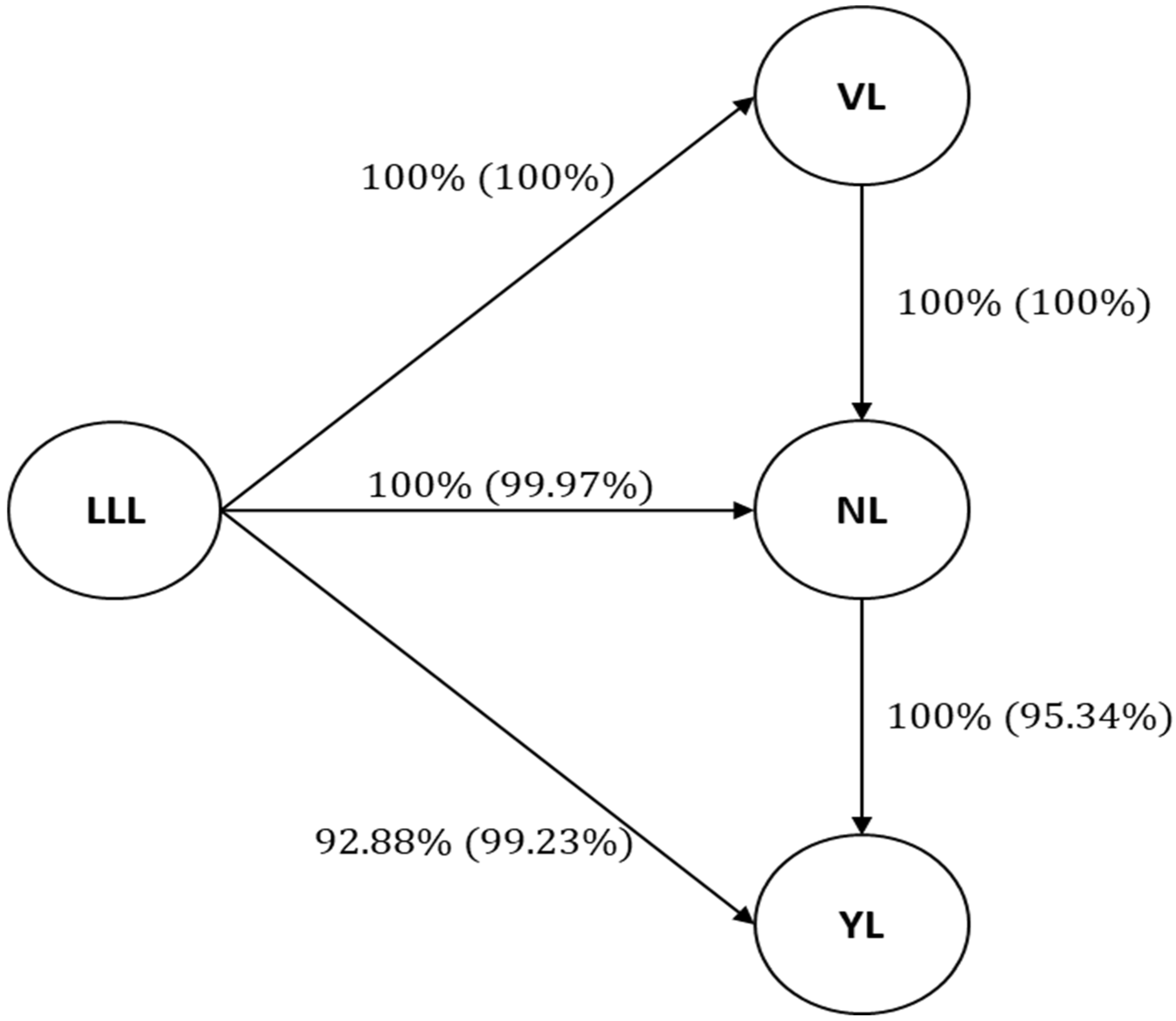
After the adjustment of the latent variables, the factor scores were corrected based on the methods [42,64]. After this correction, the latent variable scores were incorporated into the Bayesian network analysis. The Bayesian network revealed a structured interrelationship among the variables, with significant connections identified between LLL → VL, LLL → NL, LLL → YL, VL → NL and NL → YL (Table 4). The results show that the most crucial connections for model fit were LLL → NL, VL → NL, and NL → YL, as their exclusion would lead to the largest reductions in BIC. Conversely, removing LLL → VL and LLL→YL had a smaller impact on model fit (Table 4). According to Nagarajan et al. [72], Bayesian networks are defined in terms of conditional independence and probabilistic properties; however, Pearl [73] argues that a proper Bayesian network must represent the causal structure of the data. Thus, biologically, connections that have smaller effects on the global BIC may imply less important cause and effect, as is the case for LLL → VL and LLL → YL.

Suela et al. [32] used the SEM approach based on observed variables in a genome-wide association study (GWAS) in the same population as in this study. They observed direct connections from vegetative vigor to number of reproductive nodes and number of reproductive nodes to yield, which supports the findings of this work. Suela et al. [32] also highlighted the importance of the connection between vegetative vigor and number of reproductive nodes, as well as between number of reproductive nodes and yield in the general model, as indicated by BIC. Furthermore, Figure 1 shows that 100% of the bootstrap samples exhibited directed connections, which is consistent with the earlier results of Suela et al. [32]. They reported 100% and 81% frequencies of directed connections between vegetative vigor and number of vegetative nodes, and number of reproductive nodes and yield, respectively, with 68% and 100% of cases showing these directed connections, consistent with the previous findings.

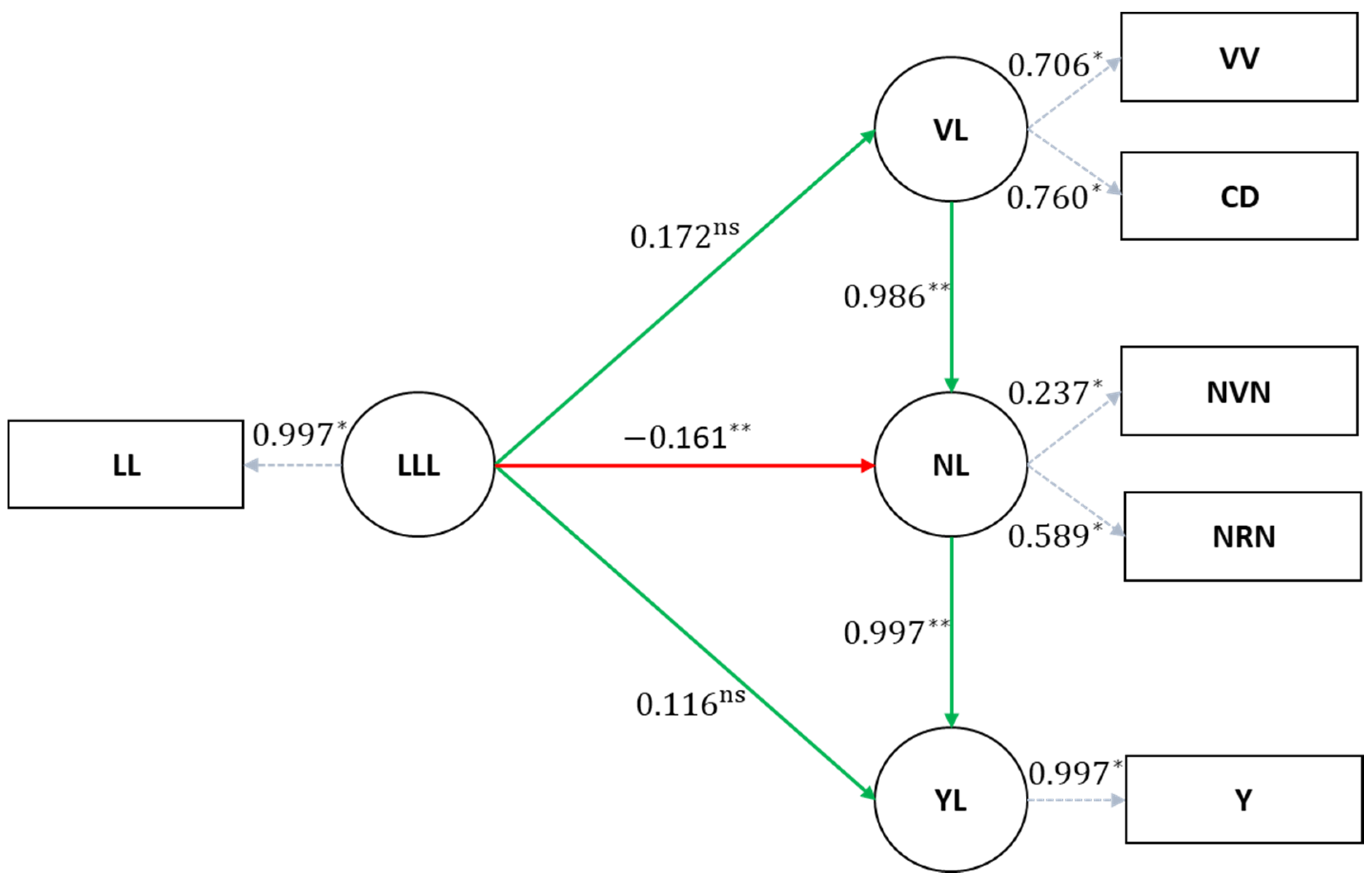
The structural coefficients, which represent cause-and-effect relationships between variables, were estimated using the SEM methodology based on the structure derived from the Bayesian networks and the previously corrected factors (Table 5 and Table 6). The paths LLL → NL, VL → NL, and NL → YL showed significant estimates of cause and effect between the variables. This contrasts with the findings of Suela et al. [32], who, without using latent variables, found non-significant coefficients for all connections.

Based on Table 3 and Table 7, it is clear that the heritability estimates of the same latent variables were different. This difference is explained by the method of obtaining each of the results, using the MTM to calculate the estimates in Table 3 and the univariate G-BLUP to calculate the estimates in Table 7. In short, these models differ in their construction, with the MTM designed to exploit the information contained in the traits of correlated indicators, while univariate models do not exploit the information of correlated traits [27].

When analyzing the results of univariate GWS, we obtained genetic parameters comparable to those reported by Sousa et al. [3] and Suela et al. [32], who used the same population. In both Sousa et al. [3] and this study, low predictive abilities and selection accuracies were observed for Y and for LL. For both the observed variables and the latent variables, we found that, for Y and LL, the gains from selection using the variables themselves or their respective latent variables were identical, at 2.11% and 0.74%, respectively. This similarity is due to the fact that the CFA was conducted using only the variable itself. Studies such as Tassone et al. [74] found yield gains for Arabica coffee ranging from 0.93 to 6.98% depending on the location and the original mean considered. However, for leaf length, the gains in the literature, as seen in the work of Chidoko et al. [75] using Arabica coffee were higher compared to those found in this study, with a value of 16.10%; however, this magnitude can be explained by the different population used, where it presented different values of genetic parameters than those found in this study.

In contrast, when VV, CD, NVN, and NRN were selected directly, the results were different from when VL and NL were selected as latent variables. Direct selection yielded gains of 1.89% for VV, 2.39% for CD, 3.76% for NVN, and 0.46% for NRN (Table 7). Carvalho et al. [76] and Tassone et al. [74] reported gains of 3% and 0.31 to 5.23% for VV, respectively. Carvalho et al. [76] and Tassone et al. [74] reported gains of 3% and −7.24 to −1.75% for CD, respectively. Thus, despite differences in the direction of the gains, there is consistency in the magnitude of the gains. However, the magnitude may vary due to differences in coffee species. In another study using Conilon coffee, Silva et al. [77] found a gain of 5.23% for the number of nodes.

On the other hand, using VL for indirect selection in VV and CD resulted in selection gains of 1.40% and 1.77%, respectively (Table 8). Similarly, selecting NL for indirect selection in NVN and NRN resulted in selection gains of 0.79% and 0.70%, respectively (Table 8). Hence, it is evident that the use of latent variables as a selection criterion guarantees gains in all the observed variables, with only a slight reduction in the gains for VV and CD, a slight reduction in the gains for NVN, and a slight increase in NRN, compared to using the observed variables themselves.

As shown in Table 5, ${\lambda }_{LLL \to NL}$, ${\lambda }_{VL \to NL}$, and ${\lambda }_{NL \to YL}$ were significant, but only MTM correlation information is required for the selection scenario [30,68]. By selecting VL and estimating the response in NVN and NRN, similar gains were achieved compared to selecting NL (Table 8). This indicates that the existing cause-and-effect relationships facilitate indirect selection for Arabica coffee node number traits in our data. In the case of Y, selecting individuals for NL and estimating the indirect effect on Y resulted in a gain of 3.51%, which is 66.35% higher than what would be achieved by selection based solely on the trait Y itself. This improvement in gain with indirect selection can be attributed to the low values of ${\mathrm{h}}^2$ and ${\mathrm{r}}_{\widehat{\mathrm{y}},\mathrm{y}}$ for the target variable (Table 7 and Table 8). It is also important to highlight that the predictive ability for NRN was negative (−0.1081) (Table 7), which reflects the low heritability and low genetic correlation of this trait with other variables included in the model. Negative predictive ability values can occur when the proportion of genetic variance is low relative to residual variance, especially for traits with limited genetic control or high environmental variability [78,79]. From a breeding perspective, this indicates that direct selection for NRN, based on genomic predictions from this model, would be unreliable and potentially misleading. Instead, indirect selection using genetically correlated traits, such as NL, may offer a more effective strategy for improving traits associated with NRN in Arabica coffee.

Interestingly, the negative effect observed from LLL to NL suggests that genotypes with longer leaves tend to produce fewer nodes, likely reflecting a physiological trade-off between resource allocation for leaf expansion and node initiation. Longer leaves typically require the greater investment of assimilates and nutrients [80,81], and they are often associated with increased internode length, leading to reduced node density along the stem. Additionally, larger leaves can increase self-shading within the canopy, limiting light interception at lower nodes and reducing meristematic activity [82]. Supporting our findings, Yirga et al. [83] also reported a negative genotypic correlation and negative effects between leaf length and number of nodes in Ethiopian Arabica coffee germplasm.

Conversely, it is important to highlight that the paths from LLL to VL and from LLL to YL were not significant in the SEM (Table 5), and this lack of effect is consistent with the Bayesian network analysis, which showed that removing these connections resulted in minimal changes in BIC values (Table 4). These findings suggest that, although LLL is structurally positioned upstream in the network, its influence on downstream traits such as YL is likely weak or indirect in this population. Therefore, these pathways do not contribute substantially to the efficiency of selection and illustrate how SEM helps filter out biologically less informative relationships.

From a practical breeding standpoint, the results presented here highlight how indirect selection via latent variables—especially NL for Y—can provide substantial genetic gains while reducing reliance on traits with low heritability or those expressed late in the plant’s development. In perennial crops such as C. arabica, where phenotyping for traits like yield is time-consuming and costly, using early measured traits (e.g., number of reproductive nodes and number of vegetative nodes) to predict target traits through SEM-based relationships can accelerate and streamline selection decisions. For instance, indirect selection using NL resulted in a 3.51% gain in yield (Y), representing a 66.35% increase compared to direct selection (2.11%), as highlighted in Table 8. These results, emphasized in Table 7 and Table 8, show that SEM-based selection strategies offer a cost-effective and operationally feasible alternative for breeding programs. Once the SEM structure is defined, the computation of latent scores can be performed using standard field measurements, making this approach scalable for routine use. Therefore, incorporating SEM into multi-trait genomic selection frameworks may significantly enhance breeding efficiency, particularly when aiming for early selection, dimensionality reduction, and increased prediction accuracy in complex trait networks.

The integration of genome-wide selection (GWS) further strengthens these advantages by enabling the early and accurate identification of superior individuals based on genomic estimated breeding values. As demonstrated by Sousa et al. [3] in Arabica coffee, GWS alone can substantially reduce breeding cycle length and operational costs by predicting complex traits before full phenotypic expression. When combined with SEM and the use of biologically meaningful latent variables such as VL and NL, this framework allows breeders to target early vegetative traits like VL to indirectly improve node-related traits (NVN and NRN) and to use NL as a key driver of yield. By prioritizing individuals with superior VL scores during early field stages, breeders can enhance genetic gains for nodal development while simultaneously shortening selection cycles by several years. Together, these strategies optimize both the speed and magnitude of genetic improvement in Arabica coffee breeding programs.

4.2. Interpretability of SEM in Biological Context

Based on the fit measures obtained from the CFA, BN, and SEM analyses, it is evident that the procedures employed were satisfactory and allowed for meaningful biological interpretation. Among these analyses, the first showed significant factor loadings in all cases, the second revealed the most robust structural relationships between the variables, and the third provided structural coefficients. However, there may be issues related to the interpretation of parameters arising from SEM in the context of a breeding program. Therefore, this section is focused on providing some explanations using the data used in this study.

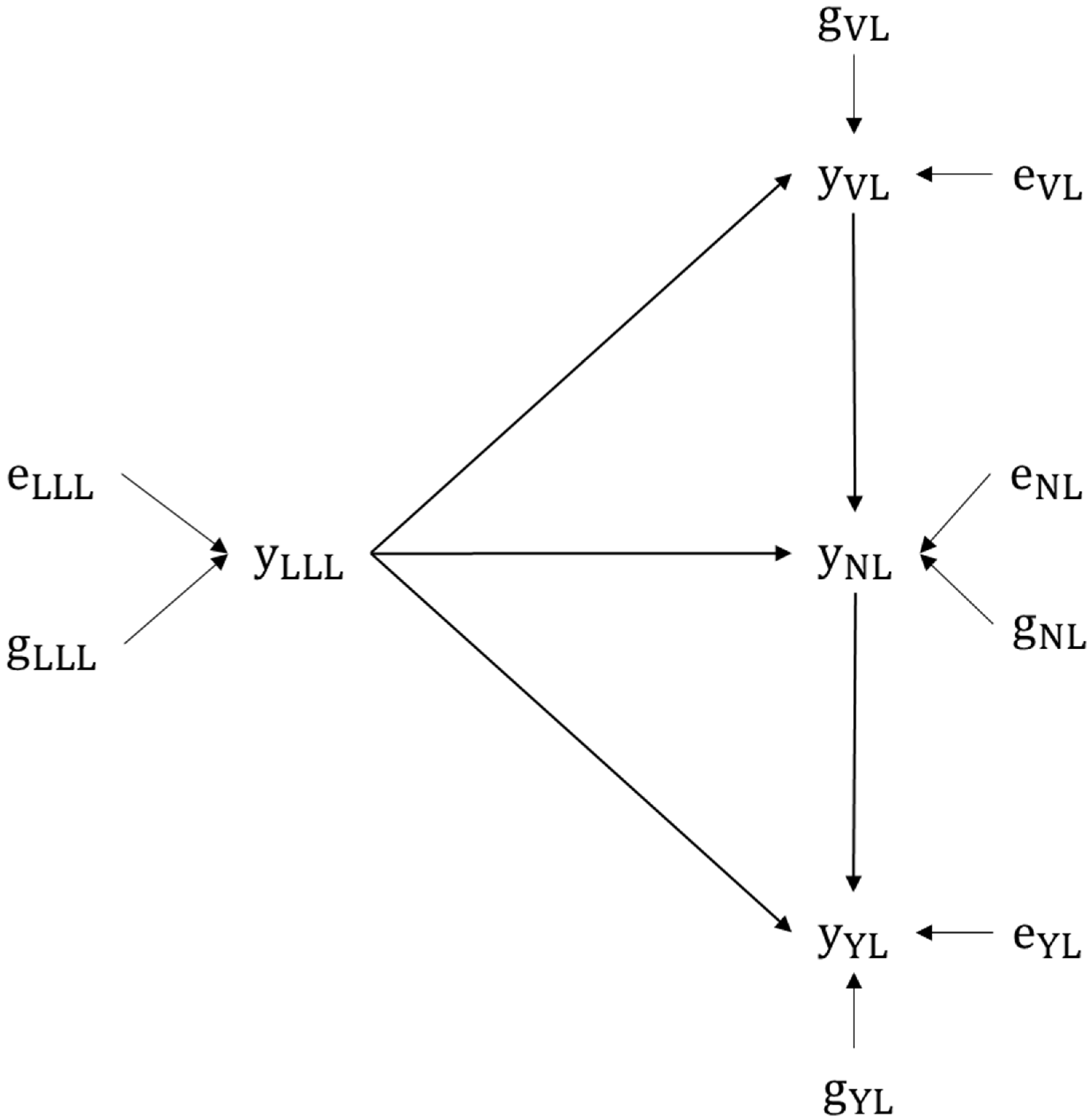
All explanations are based on the data used in this study, which are structured in the following path network (Figure 3).

Firstly, it is important to understand that the breeding values obtained from MTM and SEM can be considered equivalent (as described in Section 2.6), as long as the relationship ${\mathbf{g}}^{\mathbf{\ast }}={\mathbf{\Lambda }}^{-\mathbf{1}}\mathbf{g}$ holds, where ${\mathbf{g}}^{\mathbf{\ast }}$ is the vector of breeding values in MTM, ${\mathbf{\Lambda }}^{-1}$ is the matrix of the structural coefficients, and $\mathbf{g}$ is the vector of breeding values under SEM [33] and also due to the fact that both models produce the same joint probability distribution of phenotypes [30]. However, genetic and environmental covariances between variables can increase or decrease depending on the sign of the structural coefficient. Any changes in covariances can result in proportional changes in other genetic parameters, such as genetic correlation, environmental correlation, and heritability [68]. Algebraic equations of genetic parameters for the given path network can be found in the Text S1, as well as the estimated values for the MTM and SEM models (Table S10) according to the analysis performed in Section 2.4 and Section 2.6, which can be validated according to the equations generated according to the path network.

According to Varona and González-Recio [68], a noticeable pattern is that the higher the structural coefficient resulting from SEM, the greater the genetic correlation resulting from MTM, regardless of the genetic covariance between traits. This pattern can be observed in the significant genetic correlations from MTM (Table 3). For example, the VL $\to$ NL and NL $\to$ YL connections had the highest structural coefficient and the highest genetic correlation. Additionally, when the structural coefficient is greater than 1, it indicates that the phenotypic variance of the dependent variable can also be explained by non-genetic effects, which did not occur in this data set.

While these comparisons provide insight into the relationship between the two models using genetic parameters, it is important to understand how the breeding values should be interpreted. Statistical equivalence between the models does not necessarily imply biological equivalence. Breeding values estimated by MTM are calculated based on the existence of pleiotropy or linkage disequilibrium between QTLs and common environmental effects [68], including all additive effects of genes on the trait, even if they have a direct or indirect influence [30]. However, SEM-based breeding values consider not only common genetic and environmental effects but also non-genetic effects that arise from the phenotypic influence of another trait. These effects represent the direct and indirect effects of genes on the trait, rather than an indirect influence through the phenotypic influence of another trait [30]. In other words, breeding values are corrected for causality in SEM [68].

From the perspective of a breeding program focused on the selection of superior individuals, it is recommended to use the breeding values obtained by MTM rather than SEM [30,68]. This is because the relevant information for selecting superior individuals is given by the overall genetic effect, which is already provided by MTM without the need for SEM [30]. However, SEM analysis using latent variables offers advantages in terms of the model and the informativeness of the results. In terms of the model, SEM provides greater model parsimony compared to MTM [30]. It also offers dimensionality reduction and an improved ability to converge when dealing with complex networks of interrelationships [42]. In terms of model informativeness, SEM allows the observation of phenotypic changes resulting from causal relationships between traits and also the distinction between direct and indirect genetic effects. These changes can be understood in the context of the structural coefficient, representing a $\lambda$-unit change in the predicted variables. In addition, Valente et al. [30] pointed out that, when performing MTM, the use of different scenarios may require the construction of additional variables or the performance of new analyses, whereas SEM can handle such variations without the need for additional data processing or extended analysis time.

5. Conclusions

The findings of this study highlight the effectiveness of CFA in reducing analytical complexity while ensuring biological interpretability. Furthermore, it facilitates the estimation of causal relationships within SEM by leveraging the interrelationships identified by Bayesian network analysis. By decomposing effects into direct and indirect effects of variables, our investigation revealed that indirect selection methods, both within latent variables predicting gains in their corresponding observed variables and those predicting gains in observed variables explained by other latent variables, can enhance selection efficiency. Specifically, we observed that selecting individuals based on the latent variable VL yielded similar gains in NVN and NRN as selecting based on NL. In contrast, selecting Y based on NL resulted in a remarkable 66.35% higher gain than using the respective observed variable itself. These findings underscore the efficacy of indirect selection strategies for accurately predicting superior individuals related to traits encompassing vigor, morphology, and yield. Additionally, they shed light on the behavior of phenotypes in a recursive structure in the face of an external intervention, which can be estimated through the coefficient structure derived from SEM analysis.

References

1. United States Department of Agriculture. Coffee: World Markets and Trade; United States Department of Agriculture: Washington, DC, USA, 2024. [Google Scholar]
2. Lashermes, P.; Combes, M.C.; Robert, J.; Trouslot, P.; D’Hont, A.; Anthony, F.; Charrier, A. Molecular Characterisation and Origin of the Coffea arabica L. Genome. Mol. Gen. Genet. 1999, 261, 259–266. [Google Scholar] [CrossRef] [PubMed]
3. Sousa, T.V.; Caixeta, E.T.; Alkimim, E.R.; Oliveira, A.C.B.; Pereira, A.A.; Sakiyama, N.S.; Zambolim, L.; Resende, M.D.V. Early Selection Enabled by the Implementation of Genomic Selection in Coffea Arabica Breeding. Front. Plant Sci. 2019, 9, 1934. [Google Scholar] [CrossRef] [PubMed]
4. de Sousa, I.C.; Nascimento, M.; Silva, G.N.; Nascimento, A.C.C.; Cruz, C.D.; Silva, F.F.E.; de Almeida, D.P.; Pestana, K.N.; Azevedo, C.F.; Zambolim, L.; et al. Genomic Prediction of Leaf Rust Resistance to Arabica Coffee Using Machine Learning Algorithms. Sci. Agric. 2020, 78, e20200021. [Google Scholar] [CrossRef]
5. Adunola, P.; Tavares Flores, E.; Riva-Souza, E.M.; Ferrão, M.A.G.; Senra, J.F.B.; Comério, M.; Espindula, M.C.; Verdin Filho, A.C.; Volpi, P.S.; Fonseca, A.F.A.; et al. A Comparison of Genomic and Phenomic Selection Methods for Yield Prediction in Coffea Canephora. Plant Phenome J. 2024, 7, e20109. [Google Scholar] [CrossRef]
6. Bernardo, R.; Yu, J. Prospects for Genomewide Selection for Quantitative Traits in Maize. Crop Sci. 2007, 47, 1082–1090. [Google Scholar] [CrossRef]
7. Lorenz, A.J.; Smith, K.P.; Jannink, J.L. Potential and Optimization of Genomic Selection for Fusarium Head Blight Resistance in Six-Row Barley. Crop Sci. 2012, 52, 1609–1621. [Google Scholar] [CrossRef]
8. Das, R.R.; Vinayan, M.T.; Seetharam, K.; Patel, M.; Phagna, R.K.; Singh, S.B.; Shahi, J.P.; Sarma, A.; Barua, N.S.; Babu, R.; et al. Genetic Gains with Genomic versus Phenotypic Selection for Drought and Waterlogging Tolerance in Tropical Maize (Zea mays L.). Crop J. 2021, 9, 1438–1448. [Google Scholar] [CrossRef]
9. Persa, R.; Canella Vieira, C.; Rios, E.; Hoyos-Villegas, V.; Messina, C.D.; Runcie, D.; Jarquin, D. Improving Predictive Ability in Sparse Testing Designs in Soybean Populations. Front. Genet. 2023, 14, 1269255. [Google Scholar] [CrossRef]
10. Lopez-Cruz, M.; Dreisigacker, S.; Crespo-Herrera, L.; Bentley, A.R.; Singh, R.; Poland, J.; Shrestha, S.; Huerta-Espino, J.; Govindan, V.; Juliana, P.; et al. Sparse Kernel Models Provide Optimization of Training Set Design for Genomic Prediction in Multiyear Wheat Breeding Data. Plant Genome 2022, 15, e20254. [Google Scholar] [CrossRef]
11. Riedelsheimer, C.; Technow, F.; Melchinger, A.E. Comparison of Whole-Genome Prediction Models for Traits with Contrasting Genetic Architecture in a Diversity Panel of Maize Inbred Lines. BMC Genom. 2012, 13, 452. [Google Scholar] [CrossRef]
12. Massman, J.M.; Jung, H.J.G.; Bernardo, R. Genomewide Selection versus Marker-Assisted Recurrent Selection to Improve Grain Yield and Stover-Quality Traits for Cellulosic Ethanol in Maize. Crop Sci. 2013, 53, 58–66. [Google Scholar] [CrossRef]
13. Asoro, F.G.; Newell, M.A.; Beavis, W.D.; Scott, M.P.; Tinker, N.A.; Jannink, J.L. Genomic, Marker-Assisted, and Pedigree-BLUP Selection Methods for β-Glucan Concentration in Elite Oat. Crop Sci. 2013, 53, 1894–1906. [Google Scholar] [CrossRef]
14. Beyene, Y.; Semagn, K.; Mugo, S.; Tarekegne, A.; Babu, R.; Meisel, B.; Sehabiague, P.; Makumbi, D.; Magorokosho, C.; Oikeh, S.; et al. Genetic Gains in Grain Yield through Genomic Selection in Eight Bi-Parental Maize Populations under Drought Stress. Crop Sci. 2015, 55, 154–163. [Google Scholar] [CrossRef]
15. Larièpe, A.; Moreau, L.; Laborde, J.; Bauland, C.; Mezmouk, S.; Décousset, L.; Mary-Huard, T.; Fiévet, J.B.; Gallais, A.; Dubreuil, P.; et al. General and Specific Combining Abilities in a Maize (Zea mays L.) Test-Cross Hybrid Panel: Relative Importance of Population Structure and Genetic Divergence between Parents. Theor. Appl. Genet. 2017, 130, 403–417. [Google Scholar] [CrossRef]
16. Fang, C.; Ma, Y.; Wu, S.; Liu, Z.; Wang, Z.; Yang, R.; Hu, G.; Zhou, Z.; Yu, H.; Zhang, M.; et al. Genome-Wide Association Studies Dissect the Genetic Networks Underlying Agronomical Traits in Soybean. Genome Biol. 2017, 18, 161. [Google Scholar] [CrossRef]
17. Song, J.; Carver, B.F.; Powers, C.; Yan, L.; Klápště, J.; El-Kassaby, Y.A.; Chen, C. Practical Application of Genomic Selection in a Doubled-Haploid Winter Wheat Breeding Program. Mol. Breed. 2017, 37, 117. [Google Scholar] [CrossRef] [PubMed]
18. Suela, M.M.; Lima, L.P.; Azevedo, C.F.; De Resende, M.D.V.; Nascimento, M.; Fonseca, E.; Silva, F. Combined Index of Genomic Prediction Methods Applied to Productivity. Cienc. Rural 2019, 49, e20181008. [Google Scholar] [CrossRef]
19. Grattapaglia, D.; Vilela Resende, M.D.; Resende, M.R.; Sansaloni, C.P.; Petroli, C.D.; Missiaggia, A.A.; Takahashi, E.K.; Zamprogno, K.C.; Kilian, A. Genomic Selection for Growth Traits in Eucalyptus: Accuracy within and across Breeding Populations. BMC Proc. 2011, 5, O16. [Google Scholar] [CrossRef]
20. Younessi-Hamzekhanlu, M.; Gailing, O. Genome-Wide SNP Markers Accelerate Perennial Forest Tree Breeding Rate for Disease Resistance through Marker-Assisted and Genome-Wide Selection. Int. J. Mol. Sci. 2022, 23, 12315. [Google Scholar] [CrossRef]
21. Adunola, P.; Ferrão, M.A.G.; Ferrão, R.G.; da Fonseca, A.F.A.; Volpi, P.S.; Comério, M.; Verdin Filho, A.C.; Munoz, P.R.; Ferrão, L.F.V. Genomic Selection for Genotype Performance and Environmental Stability in Coffea Canephora. G3 Genes Genomes Genet. 2023, 13, jkad062. [Google Scholar] [CrossRef]
22. Jia, Y.; Jannink, J.L. Multiple-Trait Genomic Selection Methods Increase Genetic Value Prediction Accuracy. Genetics 2012, 192, 1513–1522. [Google Scholar] [CrossRef] [PubMed]
23. Montesinos-López, O.A.; Montesinos-López, A.; Crossa, J.; Toledo, F.H.; Pérez-Hernández, O.; Eskridge, K.M.; Rutkoski, J. A Genomic Bayesian Multi-Trait and Multi-Environment Model. G3 Genes Genomes Genet. 2016, 6, 2725–2774. [Google Scholar] [CrossRef]
24. Montesinos-López, O.A.; Montesinos-López, A.; Crossa, J.; Gianola, D.; Hernández-Suárez, C.M.; Martín-Vallejo, J. Multi-Trait, Multi-Environment Deep Learning Modeling for Genomic-Enabled Prediction of Plant Traits. G3 Genes Genomes Genet. 2018, 8, 3829–3840. [Google Scholar] [CrossRef]
25. Bhatta, M.; Gutierrez, L.; Cammarota, L.; Cardozo, F.; Germán, S.; Gómez-Guerrero, B.; Pardo, M.F.; Lanaro, V.; Sayas, M.; Castro, A.J. Multi-Trait Genomic Prediction Model Increased the Predictive Ability for Agronomic and Malting Quality Traits in Barley (Hordeum vulgare L.). G3 Genes Genomes Genet. 2020, 10, 1113–1124. [Google Scholar] [CrossRef]
26. Gaire, R.; de Arruda, M.P.; Mohammadi, M.; Brown-Guedira, G.; Kolb, F.L.; Rutkoski, J. Multi-Trait Genomic Selection Can Increase Selection Accuracy for Deoxynivalenol Accumulation Resulting from Fusarium Head Blight in Wheat. Plant Genome 2021, 15, e20188. [Google Scholar] [CrossRef] [PubMed]
27. Calus, M.P.L.; Veerkamp, R.F. Accuracy of Multi-Trait Genomic Selection Using Different Methods. Genet. Sel. Evol. 2011, 43, 26. [Google Scholar] [CrossRef] [PubMed]
28. Atanda, S.A.; Steffes, J.; Lan, Y.; Al Bari, M.A.; Kim, J.H.; Morales, M.; Johnson, J.P.; Saludares, R.; Worral, H.; Piche, L.; et al. Multi-Trait Genomic Prediction Improves Selection Accuracy for Enhancing Seed Mineral Concentrations in Pea. Plant Genome 2022, 15, e20260. [Google Scholar] [CrossRef] [PubMed]
29. Montesinos-López, O.A.; Montesinos-López, A.; Crossa, J.; Cuevas, J.; Montesinos-López, J.C.; Gutiérrez, Z.S.; Lillemo, M.; Philomin, J.; Singh, R. A Bayesian Genomic Multi-Output Regressor Stacking Model for Predicting Multi-Trait Multi-Environment Plant Breeding Data. G3 Genes Genomes Genet. 2019, 9, 3381–3393. [Google Scholar] [CrossRef]
30. Valente, B.D.; Rosa, G.J.M.; Gianola, D.; Wu, X.L.; Weigel, K. Is Structural Equation Modeling Advantageous for the Genetic Improvement of Multiple Traits? Genetics 2013, 194, 561–572. [Google Scholar] [CrossRef]
31. Paixão, P.T.M.; Nascimento, A.C.C.; Nascimento, M.; Azevedo, C.F.; Oliveira, G.F.; da Silva, F.L.; Caixeta, E.T. Factor Analysis Applied in Genomic Selection Studies in the Breeding of Coffea Canephora. Euphytica 2022, 218, 42. [Google Scholar] [CrossRef]
32. Suela, M.M.; Azevedo, C.F.; Nascimento, A.C.C.; Momen, M.; de Oliveira, A.C.B.; Caixeta, E.T.; Morota, G.; Nascimento, M. Genome-Wide Association Study for Morphological, Physiological, and Productive Traits in Coffea Arabica Using Structural Equation Models. Tree Genet. Genomes 2023, 19, 23. [Google Scholar] [CrossRef]
33. Gianola, D.; Sorensen, D. Quantitative Genetic Models for Describing Simultaneous and Recursive Relationships between Phenotypes. Genetics 2004, 167, 1407–1424. [Google Scholar] [CrossRef] [PubMed]
34. Valente, B.D.; Rosa, G.J.M. Genome-Wide Association Studies and Genomic Prediction. In Methods in Molecular Biology; Gondro, C., van der Werf, J., Hayes, B., Eds.; Humana Press: Totowa, NJ, USA, 2013; Volume 1019, pp. 449–464. ISBN 978-1-62703-446-3. [Google Scholar]
35. Momen, M.; Campbell, M.T.; Walia, H.; Morota, G. Utilizing Trait Networks and Structural Equation Models as Tools to Interpret Multi-Trait Genome-Wide Association Studies. Plant Methods 2019, 15, 107. [Google Scholar] [CrossRef] [PubMed]
36. Rosa, G.J.M.; Valente, B.D.; De Los Campos, G.; Wu, X.L.; Gianola, D.; Silva, M.A. Inferring Causal Phenotype Networks Using Structural Equation Models. Genet. Sel. Evol. 2011, 43, 6. [Google Scholar] [CrossRef] [PubMed]
37. DaMatta, F.M.; Ronchi, C.P.; Maestri, M.; Barros, R.S. Ecophysiology of Coffee Growth and Production. Braz. J. Plant Physiol. 2007, 19, 485–510. [Google Scholar] [CrossRef]
38. de Oliveira, A.C.B.; Pereira, A.A.; da Silva, F.L.; de Rezende, J.C.; Botelho, C.E.; Carvalho, G.R. Prediction of Genetic Gains from Selection in Arabica Coffee Progenies. Crop Breed. Appl. Biotechnol. 2011, 11, 106–113. [Google Scholar] [CrossRef]
39. Bernardo, R. Breeding for Quantitative Traits in Plants; Stemma Press: Woodbury, NY, USA, 2020; ISBN 9780972072434. [Google Scholar]
40. Falconer, D.S.; Mackay, T.F.C. Introduction to Quantitative Genetics, 4th ed.; Pearson: Harlow, UK, 2009. [Google Scholar]
41. Carvalho, C.H.S.d. (Ed.) Cultivares de Café; EMBRAPA: Brasília, Brazil, 2008; Available online: http://www.sapc.embrapa.br/arquivos/consorcio/publicacoes_tecnicas/Livro_Cultivares.pdf (accessed on 9 July 2024).
42. Peñagaricano, F.; Valente, B.D.; Steibel, J.P.; Bates, R.O.; Ernst, C.W.; Khatib, H.; Rosa, G.J.M. Searching for Causal Networks Involving Latent Variables in Complex Traits: Application to Growth, Carcass, and Meat Quality Traits in Pigs. J. Anim. Sci. 2015, 93, 4617–4623. [Google Scholar] [CrossRef]
43. Scutari, M. Learning Bayesian Networks with Bnlearn R Package. J. Stat. Softw. 2010, 35, 1–22. [Google Scholar] [CrossRef]
44. Scutari, M.; Denis, J.-B. Bayesian Networks with Examples in R; CRC Press: Boca Raton, FL, USA, 2014; Volume 71, ISBN 9781482225594. [Google Scholar]
45. de Oliveira Bussiman, F.; e Silva, F.F.; Carvalho, R.S.B.; Ventura, R.V.; Mattos, E.C.; Ferraz, J.B.S.; Eler, J.P.; Balieiro, J.C.d.C. Confirmatory Factor Analysis and Structural Equation Models to Dissect the Relationship between Gait and Morphology in Campolina Horses. Livest. Sci. 2022, 255, 104779. [Google Scholar] [CrossRef]
46. Pegolo, S.; Momen, M.; Morota, G.; Rosa, G.J.M.; Gianola, D.; Bittante, G.; Cecchinato, A. Structural Equation Modeling for Investigating Multi-Trait Genetic Architecture of Udder Health in Dairy Cattle. Sci. Rep. 2020, 10, 7751. [Google Scholar] [CrossRef]
47. Diniz, L.E.C.; Sakiyama, N.S.; Lashermes, P.; Caixeta, E.T.; Oliveira, A.C.B.; Zambolim, E.M.; Loureiro, M.E.; Pereira, A.A.; Zambolim, L. Analysis of AFLP Markers Associated to the Mex-1 Resistance Locus in Icatu Progenies. Crop Breed. Appl. Biotechnol. 2005, 5, 387–393. [Google Scholar] [CrossRef]
48. Sousa, T.V.; Caixeta, E.T.; Alkimim, E.R.; de Oliveira, A.C.B.; Pereira, A.A.; Zambolim, L.; Sakiyama, N.S. Molecular Markers Useful to Discriminate Coffea Arabica Cultivars with High Genetic Similarity. Euphytica 2017, 213, 607–617. [Google Scholar] [CrossRef]
49. Vieira, L.G.E.; Andrade, A.C.; Colombo, C.A.; De Araújo Moraes, A.H.; Metha, Â.; De Oliveira, A.C.; Labate, C.A.; Marino, C.L.; Monteiro-Vitorello, C.D.B.; Monte, D.D.C.; et al. Brazilian Coffee Genome Project: An EST-Based Genomic Resource. Braz. J. Plant Physiol. 2006, 18, 95–108. [Google Scholar] [CrossRef]
50. Denoeud, F.; Carretero-Paulet, L.; Dereeper, A.; Droc, G.; Guyot, R.; Pietrella, M.; Zheng, C.; Alberti, A.; Anthony, F.; Aprea, G.; et al. The Coffee Genome Provides Insight into the Convergent Evolution of Caffeine Biosynthesis. Science (80-) 2014, 345, 1181–1184. [Google Scholar] [CrossRef] [PubMed]
51. Lee, W.P.; Stromberg, M.P.; Ward, A.; Stewart, C.; Garrison, E.P.; Marth, G.T. MOSAIK: A Hash-Based Algorithm for Accurate next-Generation Sequencing Short-Read Mapping. PLoS ONE 2014, 9, e90581. [Google Scholar] [CrossRef] [PubMed]
52. Garrison, E.; Gabor, M. Haplotype-Based Variant Detection from Short-Read Sequencing. arXiv 2012, arXiv:1207.3907. [Google Scholar] [CrossRef]
53. Wiggans, G.R.; VanRaden, P.M.; Bacheller, L.R.; Tooker, M.E.; Hutchison, J.L.; Cooper, T.A.; Sonstegard, T.S. Selection and Management of DNA Markers for Use in Genomic Evaluation. J. Dairy Sci. 2010, 93, 2287–2292. [Google Scholar] [CrossRef]
54. de Resende, M.D.V. Software Selegen-REML/BLUP: A Useful Tool for Plant Breeding. Crop Breed. Appl. Biotechnol. 2016, 16, 330–339. [Google Scholar] [CrossRef]
55. Bollen, K.A. Structural Equations with Latent Variables, 1st ed.; Wiley: Hoboken, NJ, USA, 1989; Volume 1, ISBN 0471011711. [Google Scholar]
56. Whittaker, T.A.; Schumacker, R.E. A Beginner’s Guide to Structural Equation Modeling, 5th ed.; Routledge: New York, NY, USA, 2022; ISBN 9780367490157. [Google Scholar]
57. Hu, L.; Bentler, P.M. Cutoff Criteria for Fit Indexes in Covariance Structure Analysis: Conventional Criteria versus New Alternatives. Struct. Equ. Model. 1999, 6, 1–55. [Google Scholar] [CrossRef]
58. Bentler, P. Comparative Fit Indexes in Structural Models. Psychol. Bull. 1990, 107, 238–246. [Google Scholar] [CrossRef]
59. Tucker, L.R.; Lewis, C. A Reliability Coefficient for Maximum Likelihood Factor Analysis. Psychometrika 1973, 38, 421–422. [Google Scholar] [CrossRef]
60. Rosseel, Y. Lavaan: An R Package for Structural Equation Modeling. Acta Physiol. Scand. Suppl. 2012, 48, 1–36. [Google Scholar]
61. R Core Team. R: A Language and Environment for Statistical Computing; Scientific Research Publishing Inc.: Irvine, CA, USA, 2023. [Google Scholar]
62. VanRaden, P.M. Efficient Methods to Compute Genomic Predictions. J. Dairy Sci. 2008, 91, 4414–4423. [Google Scholar] [CrossRef]
63. Smith, B.J. Boa: An R Package for MCMC Output Convergence Assessment and Posterior Inference. J. Stat. Softw. 2007, 21, 1–37. [Google Scholar] [CrossRef]
64. Valente, B.D.; Rosa, G.J.M.; De Los Campos, G.; Gianola, D.; Silva, M.A. Searching for Recursive Causal Structures in Multivariate Quantitative Genetics Mixed Models. Genetics 2010, 185, 633–644. [Google Scholar] [CrossRef] [PubMed]
65. Korb, K.B.; Nicholson, A.E. Bayesian Artificial Intelligence; Chapman & Hall/CRC: Boca Raton, FL, USA, 2004; Volume 7, pp. 221–223. [Google Scholar]
66. Davidson, R.; MacKinnon, J.G. Bootstrap Tests: How Many Bootstraps? Econom. Rev. 2000, 19, 55–68. [Google Scholar] [CrossRef]
67. Covarrubias-Pazaran, G. Genome-Assisted Prediction of Quantitative Traits Using the r Package Sommer. PLoS ONE 2016, 11, e0156744. [Google Scholar] [CrossRef]
68. Varona, L.; González-Recio, O. Invited Review: Recursive Models in Animal Breeding: Interpretation, Limitations, and Extensions. J. Dairy Sci. 2023, 106, 2198–2212. [Google Scholar] [CrossRef]
69. De Kochko, A.; Campa, C.; Guyot, R.; Hamon, P.; Poncet, V.; Tranchant-Dubreuil, C.; Hamon, S.; Akaffou, S.; Andrade, A.C.; Crouzillat, D.; et al. Advances in Coffea Genomics; Academic Press: New York, NY, USA, 2010; Volume 53, ISBN 9780123808721. [Google Scholar]
70. da Silva, R.A.; Caixeta, E.T.; Silva, L.d.F.; Sousa, T.V.; Barreiros, P.R.R.M.; de Oliveira, A.C.B.; Pereira, A.A.; Barreto, C.A.V.; Nascimento, M. Identification of SNP Markers and Candidate Genes Associated with Major Agronomic Traits in Coffea Arabica. Plants 2024, 13, 1876. [Google Scholar] [CrossRef]
71. Brown, T.A. Confirmatory Factor Analysis for Applied Research, 2nd ed.; Kenny, D.A., Little, T.D., Eds.; The Guilford Press: New York, NY, USA, 2015; ISBN 1462515363. [Google Scholar]
72. Nagarajan, R.; Scutari, M.; Lèbre, S. Bayesian Networks in R with Applications in Systems Biology; Springer: New York, NY, USA, 2013; ISBN 9781461464457. [Google Scholar]
73. Pearl, J. Causality: Models, Reasoning, and Inference; Cambridge University Press: New York, NY, USA, 2009; ISBN 978-0-521-89560-6. [Google Scholar]
74. Tassone, G.A.T.; Nadaleti, D.H.S.; Carvalho, G.R.; Pereira, F.A.C.; Andrade, V.T.; Botelho, C.E. Simultaneous Selection in Coffee Progenies of Mundot Novo by Selection Indices. Coffee Sci. 2019, 14, 83–92. [Google Scholar] [CrossRef]
75. Chidoko, P.; Mahoya, C.; Tarusenga, S.; Kutywayo, D. Genetic Analysis of Coffee (Coffea Arabica L.) Genotypes in Zimbabwe Using Morphological Traits. Plant Breed. Biotechnol. 2022, 10, 212–223. [Google Scholar] [CrossRef]
76. Carvalho, H.F.; da Silva, F.L.; Resende, M.D.V.D.; Bhering, L.L. Selection and Genetic Parameters for Interpopulation Hybrids between Kouilou and Robusta Coffee. Bragantia 2019, 78, 52–59. [Google Scholar] [CrossRef]
77. Silva, V.A.; Abrahão, J.C.d.R.; Lima, L.A.; Carvalho, G.R.; Ferrão, M.A.G.; Salgado, S.M.L.; Volpato, M.L.; Botelho, C.E. Selection of Conilon Coffee Clones Tolerant to Pests and Diseases in Minas Gerais. Crop Breed. Appl. Biotechnol. 2019, 19, 269–276. [Google Scholar] [CrossRef]
78. Isidro, J.; Jannink, J.L.; Akdemir, D.; Poland, J.; Heslot, N.; Sorrells, M.E. Training Set Optimization under Population Structure in Genomic Selection. Theor. Appl. Genet. 2015, 128, 145–158. [Google Scholar] [CrossRef]
79. Resende, M.D.V.; Silva, F.F.; Lopes, P.S.; Azevedo, C.F. Seleção Genômica Ampla (GWS) via Modelos Mistos (REML/BLUP), Inferência Bayesiana (MCMC), Regressão Aleatória Multivariada e Estatística Espacial; Embrapa Florestas: Colombo, Brazil, 2012; ISBN 978-85-89119-08-5. [Google Scholar]
80. Maggs, D.H. Growth-Rates in Relation to Assimilate Supply and Demand. J. Exp. Bot. 1964, 15, 574–583. [Google Scholar] [CrossRef]
81. Westoby, M.; Baruch, Z.; Bongers, F.; Cavender-Bares, J.; Chapin, T.; Diemer, M.; Cornelissen, J.H.C.; Wright, I.J.; Reich, P.B.; Ackerly, D.D.; et al. The Worldwide Leaf Economics Spectrum. Nature 2004, 428, 821–827. [Google Scholar]
82. Rakocevic, M.; Androcioli-Filho, A. Morphophysiological characteristics of (Coffea arabica L.) in different arrangements: Lessons from a 3D virtual plant approach. Coffee Sci. 2010, 5, 154–166. [Google Scholar]
83. Yirga, M.; Gebreselassie, W.; Tesfaye, A. Correlation and Path Coefficient Analysis in Coffee (Coffea arabica L.) Germplasm Accessions in Ethiopia. Sci. Res. 2021, 9, 27. [Google Scholar] [CrossRef]
Figure 1. Path network generated from 100,000 bootstrap samples using the hill climbing algorithm. Values outside the parentheses represent strength (the percentage of bootstrap samples with an arc present or the bootstrap ratio of arc existence), and values inside parentheses represent direction (the percentage of bootstrap samples with a specific direction of arcs or the bootstrap ratio with a specific direction). YL: yield latent; VL: vegetative latent; LLL: leaf length latent; NL: nodes latent.
Agronomy 15 01686 g001
Figure 2. Proposed structural equation model (SEM) hypothesizing the relationship between yield latent (YL), vigor latent (VL), leaf length latent (LLL), and nodes latent (NL). The confirmatory factor analysis is represented by the relationship between YL, VL, LLL, and NL and the observed variables yield (Y), vegetative vigor (VV), canopy diameter (CD), leaf length (LL), number of vegetative nodes (NVN), and number of reproductive nodes (NRN); ** indicates significance according to HPD95 (relative highest 95% probability density) of SEM analysis; ns indicates no significance according to HPD95 (relative highest 95% probability density) of SEM analysis; * indicates significance according to p-value ( 0.05) of CFA analysis.
Agronomy 15 01686 g002
Figure 3. Relationship model between the variables constructed by the Bayesian network analysis, including latent variables ( y Y L , y V L , y N L , and y L L L ) influenced by genetic factors ( g Y L , g V L , g N L , and g L L L ), and residuals ( e Y L , e V L , e N L , and e L L L ).
Agronomy 15 01686 g003