Ensemble Learning-Driven and UAV Multispectral Analysis for Estimating the Leaf Nitrogen Content in Winter Wheat

Abstract

The aim of this study is to develop a rapid method for monitoring leaf nitrogen content (LNC) in winter wheat, which is essential for precise field management and accurate crop growth assessment. This study used a natural winter wheat population at Shanxi Agricultural University’s experimental base as the subject. UAV-mounted multispectral sensors collected images at jointing, heading, pre-grouting, and late grouting stages. Canopy spectral reflectance was extracted using image segmentation, and vegetation indices were calculated. Correlation analysis identified highly relevant indices with LNC. Support Vector Regression (SVR), Random Forest (RF), Ridge Regression (RR), K-Nearest Neighbors (K-NN), and ensemble learning algorithms (Voting and Stacking) were employed to model the relationship between selected vegetation indices and LNC. Model performance was evaluated using the coefficient of determination (R²) and root mean square error (RMSE). Results showed that the Voting-based ensemble learning model outperformed other models. At the pre-grouting stage, this model achieved an R² of 0.85 and an RMSE of 1.57 for the training set, and an R² of 0.82 and an RMSE of 1.64 for the testing set. This study provides a theoretical basis and technical reference for monitoring LNC in winter wheat at key growth stages using low-altitude multispectral sensors, supporting precision agriculture and variety evaluation.

1. Introduction

Wheat, as one of China’s three principal grain crops, plays a critical role in ensuring national food security and stability [1]. At present, China maintains a stable wheat supply with well-established advantageous production areas. Wheat varieties are gradually shifting from a focus on stable yields to high-yield, high-quality, and multi-resistance. Meanwhile, the market demand for high-quality specialty wheat is also increasing. The development of precision agriculture can help farmers make accurate and differentiated decisions on farming operations such as planting, fertilizer application, pest control and harvesting [2]. In recent years, with the rapid modernization of agriculture, the accuracy of differentiated management has continuously improved. Obtaining crop nutrient information quickly, accurately, promptly, and efficiently is of great significance for high-yield cultivation and the selection and breeding of superior varieties [3].

Since soil nutrients alone cannot sustain high yields, fertilization is necessary to improve crop productivity. Among nutrients, nitrogen is particularly critical for regulating wheat’s physiological functions [4,5]. However, the widespread overuse of nitrogen fertilizers has led to significant risks, including water pollution, soil acidification, and increased production costs [6,7]. Consequently, the precise application of nitrogen to improve nitrogen use efficiency has received increasing attention [8].

Leaf nitrogen content (LNC) is an important phenotypic indicator reflecting the nitrogen nutritional status of crops and provides valuable guidance for scientific fertilization and the selection of superior cultivars [9]. However, traditional chemical methods for determining LNC are destructive and time-consuming, making them unsuitable for large-scale, real-time monitoring [10,11]. In recent years, non-destructive monitoring techniques based on remote sensing have attracted increasing attention [12]. Among them, unmanned aerial vehicle (UAV) remote sensing has shown great potential in collecting crop spectral information due to its high spatiotemporal resolution and flexible data acquisition capabilities, and it has been widely applied in LNC estimation model development [13,14].

Previous studies have achieved promising results in estimating LNC using regression models based on spectral or texture features extracted from multispectral images [15,16]. However, most of these studies pay limited attention to the challenges posed by complex field backgrounds. Accurately extracting canopy reflectance from UAV-based multispectral images is challenging due to background interference from heterogeneous soil textures, fluctuating illumination, and weeds, often requiring labor-intensive manual segmentation [17,18]. Traditional threshold segmentation methods are difficult to adapt to changing environmental conditions, complicating the precise extraction of winter wheat canopy spectral reflectance [19,20]. Additionally, estimating LNC through UAV remote sensing depends on robust models linking spectral features with nitrogen content, but traditional machine learning algorithms often fail to capture the complex, dynamic nature of crop growth, limiting model accuracy and generalizability [21,22].

To address the above issues, this study proposes an approach for estimating LNC in winter wheat by integrating image segmentation with ensemble modeling. At the image processing level, machine learning-based segmentation algorithms are used to enhance the accuracy of canopy reflectance extraction under complex field backgrounds. At the modeling level, ensemble learning strategies are used to improve the robustness and generalizability of the estimation model.

The specific research objectives are as follows: (1) Integrate canopy image segmentation techniques to effectively distinguish plant canopy from soil background, improving the accuracy of canopy reflectance extraction from UAV multispectral images. (2) Compare the performance differences between traditional machine learning algorithms and ensemble learning algorithms, selecting the most suitable algorithm. (3) Based on the above, develop a more precise model for estimating winter wheat LNC.

2. Materials and Methods

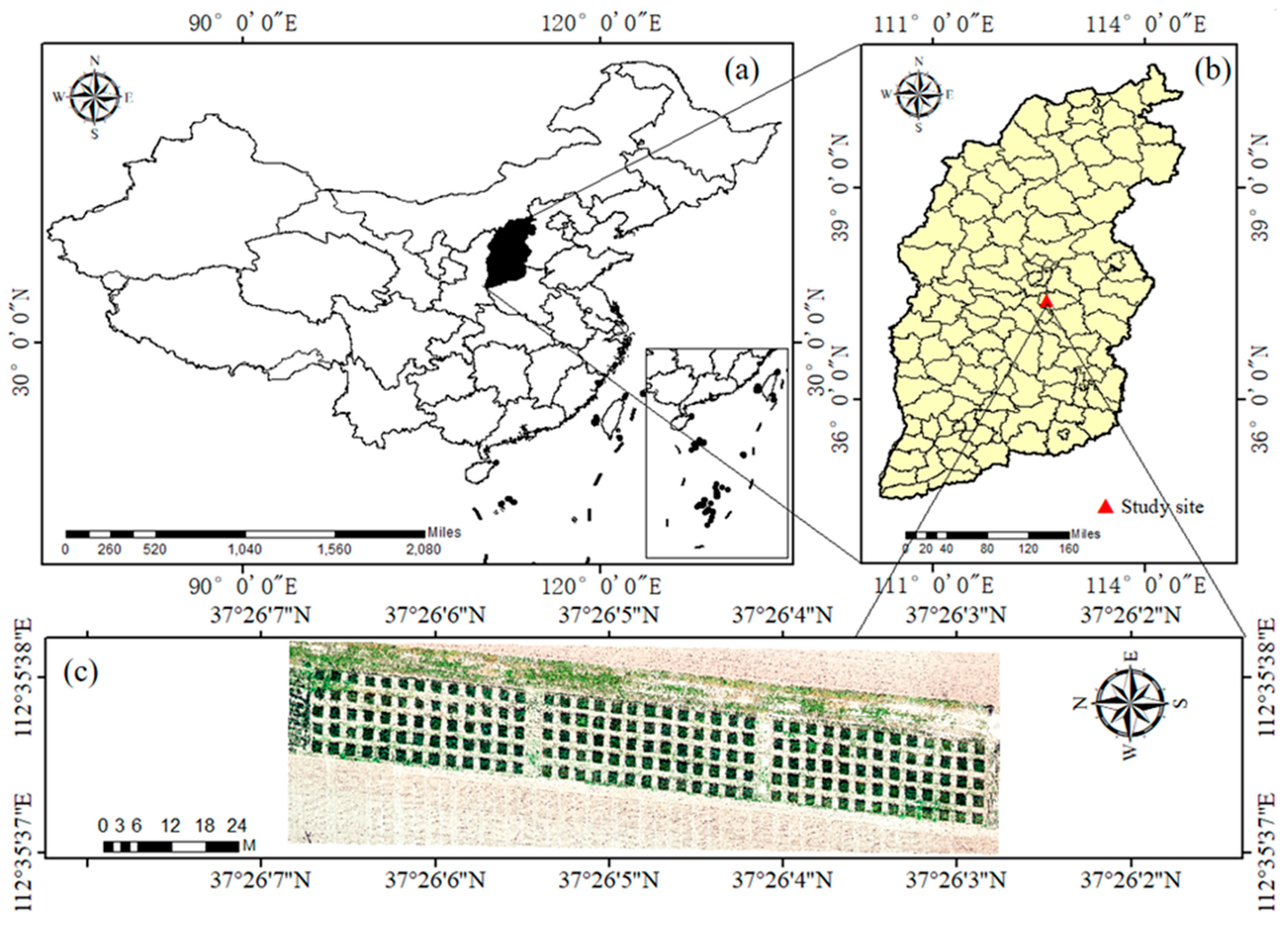
2.1. Overview of the Experimental Area and Experimental Design

The study site is located in Taigu District of Jinzhong City, Shanxi Province, China (112°28′–113°01′ E, 37°12′–37°32′ N), situated in the northeastern part of Jinzhong City, covering an area of approximately 105 km² (Figure 1). The area is located in a warm temperate zone and has a continental monsoon climate, characterized by warmer spring temperatures compared with autumn, hot and rainy summers, and long, cold winters. The annual average temperature is 9.8 °C, the frost-free period lasts about 175 days, and the average annual precipitation is 462.9 mm. The area has well-developed agricultural infrastructure, providing favorable conditions for field trials.

This study adopts a split-plot experimental design. The main plots consist of three nitrogen application levels, with average application rates of 0 kg/hm², 100 kg/hm², and 200 kg/hm² for the three large experimental units from right to left (

Table 1. Fertilizer application at Mengjiacun experimental base of Shanxi Agricultural University.

Treatment	Fertilizer Rate (kg/hm2)
	N	P2O5	K2O
N0	0	120	120
N1	100	120	120
N2	200	120	120

Note: In total, 50 per cent of the nitrogen fertilizer is used as a base fertilizer and the other 50 per cent as a follow-on fertilizer.

). Each main plot contains 65 different wheat varieties, yielding a total of 195 subplots. These comprise 65 distinct winter wheat populations representing a range of genotypes, including landraces, elite cultivars, new varieties, core germplasm, and introduced foreign lines. Each subplot covers an area of 3 m² (1.5 m × 2 m). Phosphate and potassium fertilizers were applied at a baseline rate of 120 kg/hm². Winter wheat was sown on 10 October 2022, and all subsequent field management followed the local high-yield cultivation standards.

The study was conducted from October 2022 to June 2023, covering key growth stages of winter wheat, including jointing (16 April ), heading (13 May), pre-grouting (22 May), and late grouting (6 June). Remote sensing data of the winter wheat canopy were obtained by a multispectral camera mounted on UAV under sunny weather conditions with wind speeds below grade 3. Simultaneously, samples of winter wheat plants were collected. At each sampling time, representative plants with uniform growth were selected from the central part of each experimental plot. After chemical desiccation and drying treatment, the nitrogen content of the leaves was determined.

2.2. Data Handling

Field sampling for determining the LNC of winter wheat was conducted at four key time points during the growing season: 16 April, 13 May, 22 May, and 6 June 2023. At each time point, winter wheat plants exhibiting uniform growth were randomly selected from each sampling area. The sampled plants were rinsed with clean water and then separated into stems and leaves. The leaf and stem samples were placed into labeled sample bags separately. To inactivate enzymes, the samples were initially dried at 105 °C for 30 min in an oven. Subsequently, the oven temperature was adjusted to 80 °C, and the samples were dried to a constant weight. After drying, the leaf samples were ground into a fine powder. Total nitrogen content was then determined using the Kjeldahl method, and measurements were recorded with a fully automated chemical analyzer.

2.3. Image Preprocessing

The experiment utilized a DJI Phantom 4 Pro drone equipped with a RedEdge-MX dual-camera multispectral imaging system (Figure 2). This sensor captures five spectral bands: blue (450 ± 16 nm), green (560 ± 16 nm), red (650 ± 16 nm), red-edge (730 ± 16 nm), and near-infrared (840 ± 16 nm). Data acquisition was conducted at key winter wheat growth stages, including jointing, heading, pre-grouting, and late grouting.

To ensure the reliability and accuracy of UAV-based remote sensing data, all flights were conducted under sunny, cloud-free conditions between 10:00 and 14:00 local time. The UAV followed a bow-shaped flight path, with 80% forward (heading) overlap and 70% side overlap. The flight altitude was maintained at 25 m above ground level. Radiometric calibration panels were photographed before and after each flight to facilitate subsequent image correction. Additionally, flight altitude and performance consistency were assessed before and after each mission to minimize variability.

As UAV-acquired orthophotos are susceptible to geometric and radiometric distortions caused by physical deviations and environmental conditions such as sunlight, preprocessing of the raw multispectral imagery was essential. Image preprocessing included stitching, radiometric correction, and cropping to improve spatial accuracy and spectral consistency. Following these steps, canopy reflectance was extracted from each plot using a threshold-based segmentation method. Subsequently, vegetation indices of winter wheat were calculated based on the extracted spectral reflectance values of individual bands.

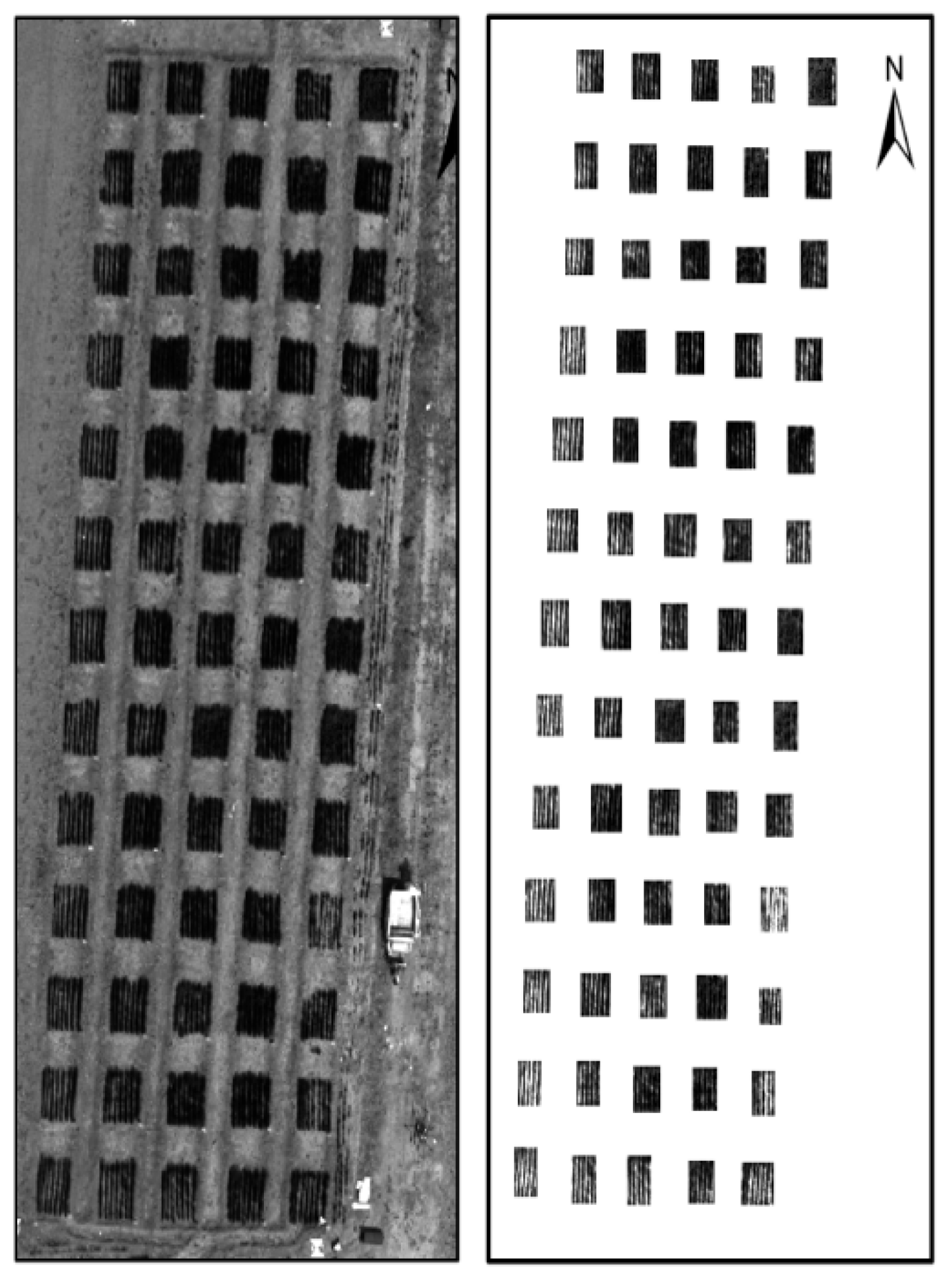
2.4. Canopy Image Segmentation

2.4.1. Introduction to Image Algorithms

To improve the accuracy of canopy–background segmentation in UAV-acquired multispectral images, this study employed two widely used machine learning algorithms—Random Forest (RF) and Support Vector Machine (SVM). Each method was used to build a pixel-level classifier for differentiating winter wheat canopy from soil background.

Random Forest (RF)

The Random Forest algorithm is an ensemble learning method that constructs a collection of decision trees—typically ranging from tens to thousands—through a process known as bootstrap aggregating (Bagging). In each iteration, a training dataset is generated via resampling using the bootstrap method, and a decision tree is constructed by randomly selecting a subset of features for node splitting. The final prediction is determined by majority voting among all trees [23].

Support Vector Machine (SVM)

SVM is a binary classification model that seeks to identify the optimal hyperplane with maximum margin separation between classes in the feature space. It can be extended to handle nonlinear classification problems by using kernel functions, such as radial basis function (RBF) and polynomial kernels. SVMs exhibit strong generalization capability due to their margin maximization strategy and inherent regularization. Additionally, they are robust to outliers and noise in the input data [24].

Canopy Segmentation Workflow:

Based on the above machine learning models, the canopy–background segmentation process was conducted as follows:

(1) Training Dataset Preparation: Training samples were manually labeled from UAV multispectral images to serve as ground truth.

(2) Model Training: The RF and SVM classifiers were trained using the labeled samples.

(3) Canopy Segmentation: The trained classifiers were applied to test images for automated canopy–background segmentation.

(4) Post-Processing: Segmentation results were refined using morphological noise reduction techniques to remove small artifacts and enhance spatial continuity.

(5) Performance Evaluation: The segmentation results obtained from both RF and SVM models were quantitatively and visually compared against manually segmented reference images to assess accuracy.

2.4.2. Image Segmentation Algorithm Specific Steps

Key Feature Extraction

Multispectral images provide rich spectral information beyond that of conventional RGB images by capturing reflectance or radiance values across multiple discrete spectral bands. This enhanced spectral detail enables more effective segmentation of the winter wheat canopy, particularly for distinguishing green vegetation from weeds and soil background.

To leverage this advantage, various vegetation indices (VIs) derived from multispectral reflectance data are widely used as key features for vegetation monitoring and canopy segmentation. Among these indices, the Normalized Difference Vegetation Index (NDVI) is the most commonly employed indicator of vegetation growth and cover. NDVI effectively reflects the amount of photosynthetically active radiation absorbed by crops and shows a strong correlation with physiological characteristics of vegetation.

The Enhanced Vegetation Index (EVI) further improves the description of biophysical canopy structure by reducing saturation effects in high biomass regions and minimizing soil background noise, making it more reliable in dense vegetation conditions.

The Modified Soil-Adjusted Vegetation Index (MSAVI) enhances vegetation signal extraction under mixed vegetation and soil environments by compensating for soil background effects, thus providing more accurate information in heterogeneous landscapes.

Based on these considerations, the key features selected for multispectral image analysis in this study include reflectance values of the five spectral channels—red (R), green (G), blue (B), near-infrared (NIR)—and the vegetation indices, the NDVI, EVI, and MSAVI. The vegetation indices are calculated as follows:

$$NDVI={\displaystyle \frac{(NIR-R)}{\left(NIR+R\right)}}$$

(1)

$$EVI=2.5\left({\displaystyle \frac{NIR-R}{NIR+6R-7.5B+1}}\right)$$

(2)

$$MSAVI={\displaystyle \frac{2NIR+1-\sqrt{{\left(2NIR+1\right)}^2-8(NIR-R)}}{2}}$$

(3)

where NIR, R, and B correspond to the near-infrared band, red band, and blue band, respectively.

Construction of Training Dataset

Due to the combined effects of varying illumination conditions, complex soil backgrounds, and the presence of weeds in winter wheat field trials, it is essential that the Support Vector Machine (ROI) used for training contains representative image elements encompassing these diverse natural conditions. This ensures the resulting model is robust and adaptable across different scenarios. In this study, the ROI consists of two classes: winter wheat canopy (labeled as 0) and background (labeled as 1). The spectral reflectance values of each pixel within the ROI, extracted from the multispectral images, together with vegetation indices calculated from these reflectance values, constitute the feature set used to build the spectral reflectance training dataset.

Classifier Construction and Biplot Generation

The decision tree in this study was trained by classification and regression trees (CART) algorithm using key features to train the decision tree model. The decision tree is optimized using cross-validation to determine the number of smallest leaf nodes in order to improve classifier efficiency, where the two dataset validation results set the optimal smallest leaf node parameter as the default value. The maximum tree depth ntree was set to 500 by default in the parameters of the Random Forest algorithm, and the default value of mtry was 2 [25]. The kernel function chosen for the SVM in the study was radial basis functions (RBFs), and the optimal penalty coefficient C was determined to be 0.25 using a cross-validated grid search, and the function parameter g to be 10. In order to compare the effectiveness of multiple machine learning models for segmentation of winter wheat canopies, the multispectral test images were segmented using two of the constructed classifier models, and then the classifier algorithms that had the best results were used to segment the multispectral reflectance image for canopy–background segmentation. Each pixel value was classified as a winter wheat canopy value of 0 or a background value of 255, and then the binary image generated by the models was subjected to noise reduction by spatial filtering to obtain the final binary image (Figure 3).

In order to further compare the performance of the two different classifiers, this paper adopts Accuracy, Percentage of Missing Segmentation (PMS), and Percentage of Wrong Split (PWS) as the evaluation metrics for segmentation precision. The definitions of these metrics are as follows:

$$Accuracy={\displaystyle \frac{TP+TN}{TP+TN+FP+FN}}\times 100\%$$

(4)

$$PMS={\displaystyle \frac{FN}{TP+FN}}\times 100\%$$

(5)

$$PWS={\displaystyle \frac{FP}{TN+FP}}\times 100\%$$

(6)

In these formulas, Accuracy is the segmentation accuracy, PMS is the proportion of missed segmentations, and PWS is the proportion of wrong splits. TP denotes correctly predicted target instances, TN denotes correctly predicted background instances, FP denotes background instances incorrectly predicted as target instances, and FN denotes target instances incorrectly predicted as background instances.

In the UAV-acquired winter wheat canopy images, varying lighting conditions and the presence of different types of weeds, in addition to soil interference, introduce significant challenges to canopy segmentation. The results indicate (

Table 2. Comparison of threshold segmentation results.

Model	Threshold	Accuracy/%	PMS/%	PWS/%
RF	NDVI	90.11	12.18	31.66
	EVI	85.63	26.93	48.29
	MSAVI	87.45	22.87	29.65
SVM	NDVI	86.29	17.28	57.96
	EVI	81.79	28.34	50.42
	MSAVI	82.06	25.37	18.58

) that the NDVI-based threshold segmentation method, combined with the RF algorithm, can more completely segment winter wheat plants. In contrast, although thresholding methods based on other vegetation indices can effectively separate the wheat canopy from the soil, their higher omission rates result in incomplete segmentation, thereby affecting the accuracy and completeness of the results. Therefore, in this paper, the threshold segmentation method based on the use of NDVI vegetation index under the RF algorithm is selected as a prerequisite for subsequent data processing.

2.5. Vegetation Index Selection

Vegetation indices (VIs) are mathematical combinations of spectral reflectance values across different wavelength bands, widely used to effectively assess crop growth status. Currently, VIs has been extensively applied in the estimation of various crop traits, including LNC, leaf area index, chlorophyll concentration, biomass, and yield. In this study, based on a comprehensive review of previous research and the data characteristics of the present experiment, 9 vegetation indices were selected for monitoring the LNC of winter wheat using UAV multispectral data. The ENVI 5.6 software was used to extract the measurement area from each experimental plot after image segmentation, and the average reflectance of all pixels within each region was calculated to represent the canopy reflectance of the plot. These average reflectance values were then used to compute the corresponding vegetation indices. The detailed formulas for each vegetation index are presented in

Table 3. Vegetation index.

Type of Vegetation Index	Calculation Formula	Source
NDVI	${\displaystyle \frac{{\rho }_{Nir}-{\rho }_{Red}}{{\rho }_{Nir}+{\rho }_{Red}}}$	[26]
GRVI	${\displaystyle \frac{{\rho }_{green}-{\rho }_{red}}{{\rho }_{green}{+\rho }_{red}}}$	[27]
SAVI	${\displaystyle \frac{(1+0.16)({\rho }_{Nir}-{\rho }_{Red})}{{\rho }_{Nir}+{\rho }_{Red}+0.16}}$	[28]
GNDVI	${\displaystyle \frac{{\rho }_{Nir}-{\rho }_{Green}}{{\rho }_{Nir}+{\rho }_{Green}}}$	[29]
SIPI	${\displaystyle \frac{{\rho }_{Nir}-{\rho }_{bliue}}{{\rho }_{Nir}-{\rho }_{red}}}$	[30]
NDRE	${\displaystyle \frac{{\rho }_{Nir}-{\rho }_{Red-edge}}{{\rho }_{Nir}+{\rho }_{Red-edge}}}$	[31]
RDVI	${\displaystyle \frac{{\rho }_{Nir}-{\rho }_{Red}}{\surd {(\rho }_{Nir}+{\rho }_{Red})}}$	[32]
EVI	$2.5 \ast {\displaystyle \frac{{(\rho }_{Nir}-{\rho }_{Red})}{{\rho }_{Nir}+6 \ast {\rho }_{Red}-7.5{\rho }_{Blue}+1}}$	[33]
CIred-edge	${\displaystyle \frac{{\rho }_{Nir}}{{\rho }_{Red-edge}}}-1$	[34]

.

2.6. Model Building

2.6.1. Random Forests

The Random Forest (RF) model, originally proposed by Breiman, employs the bagging (bootstrap aggregating) technique to integrate multiple decision trees into an ensemble learning framework. Compared to a single decision tree, RF combines a collection of classification and regression trees (CARTs), effectively mitigating the low accuracy and high variance associated with individual CART models. This ensemble approach enhances the model’s generalization ability and yields more accurate and stable predictions. Each decision tree in the forest is trained on a bootstrap sample—a randomly selected subset of the training data with replacement—while the remaining samples, referred to as out-of-bag (OOB) samples, serve as an internal testing set to estimate prediction error and assist in assessing feature importance. The contribution of each input feature to the prediction is quantified by the RF variable importance metric. RF is particularly robust against noise and overfitting compared to other machine learning algorithms [35]. In this study, a grid search was employed to optimize hyperparameters, adjusting the number of trees from 100 to 1000 in increments of 100, and tuning the maximum tree depth from 2 to 30 in increments of 5.

2.6.2. Ridge Regression

Ridge Regression (RR), also known as Tikhonov regularization, is a technique specifically designed to address issues in covariate data analysis, particularly when the number of variables exceeds the number of observations or when predictor variables exhibit high multicollinearity. Ridge regression is an extension of the ordinary least squares (OLS) estimation method. In standard OLS regression, model parameters are estimated by minimizing the sum of squared residuals. However, in the presence of strong covariance among predictor variables, OLS estimates can become unstable or even non-identifiable. Ridge regression overcomes this limitation by introducing a penalty term, commonly referred to as the regularization parameter, which shrinks coefficient estimates toward zero, thereby stabilizing the solution at the cost of introducing a small bias [36]. The objective function of ridge regression minimizes the sum of squared residuals augmented by this regularization term, and can be formally expressed as

$$J\left(\beta \right)={\sum }_{i=1}^n{(y_i-X_I\beta )}^2+\lambda {\sum }_{j=1}^p{\beta }_j^2$$

(7)

where $y_i$ is the observation, $X_I$ is the vector of row i in the design matrix representing the predictor variables for the ith observation, $\beta$ is the vector of model parameters, $\lambda$ is the regularization parameter controlling the strength of the regularization term, and $p$ is the number of predictor variables.

2.6.3. K-Nearest Neighbor

K-Nearest Neighbor (K-NN) is a supervised learning algorithm based on a distance metric, applicable to both classification and regression tasks. The core idea is that for a sample point to be predicted, the K-Nearest Neighbors are selected by calculating the distance between the sample point and all the points in the training set. The output for the predicted point is then determined based on the characteristics of these neighbors, such as majority voting or averaging [37]. K-NN is a lazy learning algorithm because it does not generate an explicit model during the training phase; instead, it utilizes the entire training dataset for computation during the prediction phase. In this study, the Euclidean distance is used to calculate the distance between data points. The Euclidean distance $d$ between two points x = (x₁, x₂, …, x_n) and y = (y₁, y₂, …, y_n) in an n-dimensional space is defined as

$$d\left(x,y\right)=\sqrt{\sum _{i=1}^n{(x_i-y_i)}^2}$$

(8)

The K-NN algorithm is known for its intuitiveness and ease of implementation, and is suitable for classification and regression tasks in small datasets and low-dimensional feature spaces. However, its high computational complexity and sensitivity to noise perform poorly on large-scale, high-dimensional data. The performance of K-NN can be effectively improved by adjusting the K-value, using a suitable distance metric (e.g., Minkowski distance), and preprocessing the data.

2.6.4. Support Vector Regression

Support Vector Regression (SVR) is a regression method based on Support Vector Machines (SVMs), which is similar in principle to linear regression, but with higher accuracy and generalization. SVR models the regression process by finding an optimal hyperplane in two dimensions. Since this optimal hyperplane only considers points at the edges around the training set, the model effectively avoids overfitting the data points. At the same time, the complexity control parameter based on the reprojection error as a penalty term can well regulate the flexibility of the regression model.

2.6.5. Stacking Model

Stacking, or stacked generalization, is an ensemble learning technique that combines the predictive capabilities of multiple base models to improve overall performance. The process involves two primary stages: first, multiple diverse base learners (e.g., classifiers or regressors) are trained on the dataset; second, a higher-level model, known as the meta-learner. This paper adopts the four basic models mentioned in the previous text, namely Random Forest (RF), Ridge Regression (RR), K-Nearest Neighbor (K-NN), and Support Vector Regression (SVR), as the basic learners. Is trained using the outputs (predictions) of the base learners as its input features. The meta-learner then generates the final prediction [38].

Stacking distinguishes itself from other ensemble methods, such as Bagging and Boosting, by learning how to optimally combine different models rather than relying on uniform aggregation (e.g., voting or averaging). This framework allows the ensemble to leverage the strengths and mitigate the weaknesses of individual learners, capturing complex patterns that may be overlooked by any single model.

While Stacking can significantly enhance model performance, especially in heterogeneous ensembles, it also introduces additional complexity and computational cost. Furthermore, it carries a higher risk of overfitting, particularly when applied to small or imbalanced datasets. Therefore, rigorous cross-validation, careful model selection, and hyperparameter tuning are essential to ensure robust generalization and prevent overfitting.

2.6.6. Voting Model

Voting, is an intuitive and effective method in integrated learning. The core idea is to improve overall performance by combining the predictions of multiple models. In Voting integration, each model gives its own prediction based on the input data, and then these predictions are aggregated in some way to produce a final prediction [39].

Voting models are usually categorized into hard and soft voting. Hard voting means that each model outputs only a label of the most likely categories and then votes based on these labels to select the category with the most votes as the final prediction. Soft voting, on the other hand, allows the model to output a probability or confidence level for each category and then vote on a weighted basis based on those probabilities or confidence levels to obtain the final prediction.

The advantage of hard voting is that it is simple, intuitive and easy to implement. However, since it only considers the labels of the categories predicted by the model and does not make use of the model’s probability or confidence information for each category, it may not be optimal in some cases. Soft voting, on the other hand, is able to make full use of the probability or confidence information of the model outputs, combining the predictions of different models in a weighted way, and usually achieves better performance.

2.7. Modeling Evaluation

In this paper, a five-fold cross-validation approach to modeling was used for model construction, with 70% of the sample size for each growth period randomly selected for the training set (n1 = 137) and the remaining 30% of the samples used for the testing set (n2 = 58) prior to the construction of each model.

In order to evaluate the performance of the model, this study adopts three commonly used metrics: the coefficient of determination (R-Square, R²), the root mean square error (RMSE), and the mean absolute error (MAE). R² effectively quantifies the degree of fit between the estimated and actual values, ranging from 0 to 1. The closer the result is to 1, the better the fit and the higher the model’s accuracy; conversely, lower values indicate a weaker fit. The calculation method is shown in the following formula:

$$R^2={\displaystyle \frac{1-\sum _{i=1}^n{\left(y_i-x_i\right)}^2}{\sum _{i=1}^n{\left(y_i-\widehat{y}\right)}^2}}$$

(9)

RMSE measures the error between predicted and observed values, with results ranging from 0 to 1. The closer the RMSE is to 0, the smaller the error and the better the fit. Conversely, larger RMSE values imply lower precision. Its formula is as follows:

$$RMSE=\sqrt{{\displaystyle \frac{\sum _{i=1}^n{\left(x_i-y_i\right)}^2}{n}}}$$

(10)

MAE, as a measure of prediction deviation for regression models, reflects the average absolute difference between predicted and observed values. It is a key indicator for assessing model stability. The lower the MAE value, the closer the prediction results are to the actual observations, indicating a higher prediction performance. Conversely, higher MAE values imply lower prediction stability and accuracy.

$$MAE={\displaystyle \frac{1}{n}}\sum _{i=1}^n\left|x_i-y_i\right|$$

(11)

Here n denotes the total number of samples; $x_i$ the predicted value; $y_i$ the observed value; and $\widehat{y}$ the mean of the observed values.

3. Results and Analysis

3.1. Variable Screening and Statistical Analysis

3.1.1. Descriptive Statistical Analysis

In this study, a total of 780 measurements of LNC in winter wheat was obtained across four growth stages: jointing, heading, pre-grouting, and late grouting. The samples were randomly divided into a training set (70%) and a testing set (30%). Descriptive statistics of the LNC values for both sets are presented in

Table 4. Descriptive statistical analysis.

Period of Fertility	Datasets	Sample	Average	Kurtosis	Skewness	Minimum	Maximum
Jointing stage	Total	195	32.870	0.624	0.357	22.174	43.278
	Train	137	33.212	0.603	0.581	23.145	43.278
	Test	58	33.672	0.722	0.492	22.174	41.150
Heading stage	Total	195	36.676	0.535	0.367	30.170	45.101
	Train	137	38.302	0.501	0.604	34.332	45.101
	Test	58	32.832	0.493	0.680	30.170	34.327
Pre-grouting stage	Total	195	30.692	0.706	0.272	25.065	36.914
	Train	137	32.100	0.875	0.491	29.038	36.914
	Test	58	27.361	1.102	0.309	25.065	28.988
Late grouting stage	Total	195	22.392	0.651	0.426	15.122	31.661
	Train	137	24.447	0.812	0.646	20.148	31.661
	Test	58	17.531	1.186	0.583	15.122	20.100

.

At the jointing stage, LNC values ranged from 22.174 to 43.278 mg/g, with a mean of 32.870 mg/g. At the heading stage, the range was 30.170 to 45.101 mg/g, with a mean of 36.676 mg/g. During pre-grouting stage, LNC values ranged from 25.065 to 36.914 mg/g, with a mean of 30.692 mg/g. At the late grouting stage, values ranged from 15.122 to 31.661 mg/g, and the mean was 22.392 mg/g. The skewness values were close to zero and kurtosis values indicated moderate peakedness, suggesting that the data approximately followed a normal distribution. Furthermore, both the training and testing sets demonstrated near-normal distributions, indicating that the datasets are suitable for subsequent modeling analyses.

3.1.2. Z-Score Outlier Elimination

The Z-score method is a statistical technique commonly used for outlier detection. It is based on the properties of the standard normal distribution and evaluates the degree of deviation of a data point from the mean of the dataset, expressed in terms of standard deviations. In a standard normal distribution, approximately 68% of data points fall within one standard deviation from the mean, 95% within two standard deviations, and 99.7% within three standard deviations. Therefore, if a data point has a large absolute Z-score—meaning it deviates from the mean by several standard deviations—it is likely to be considered an outlier. The Z-score is calculated using the following formula:

$$Z={\displaystyle \frac{(X-\mu )}{\sigma }}$$

(12)

where $X$ is a data point in the dataset, $\mu$ is the mean (average) of the dataset, and $\sigma$ is the standard deviation of the dataset. $Z$ is the Z-score of the data point $X$. The data point X is the Z-score of the dataset.

Based on the Z-score method described above, outliers in the LNC values across the four growth stages of winter wheat were identified and removed. This step was taken to exclude anomalous data points that may have arisen due to operational errors or human factors. The elimination of these abnormal values helps to enhance the quality of the dataset and improve the accuracy and robustness of subsequent prediction models.

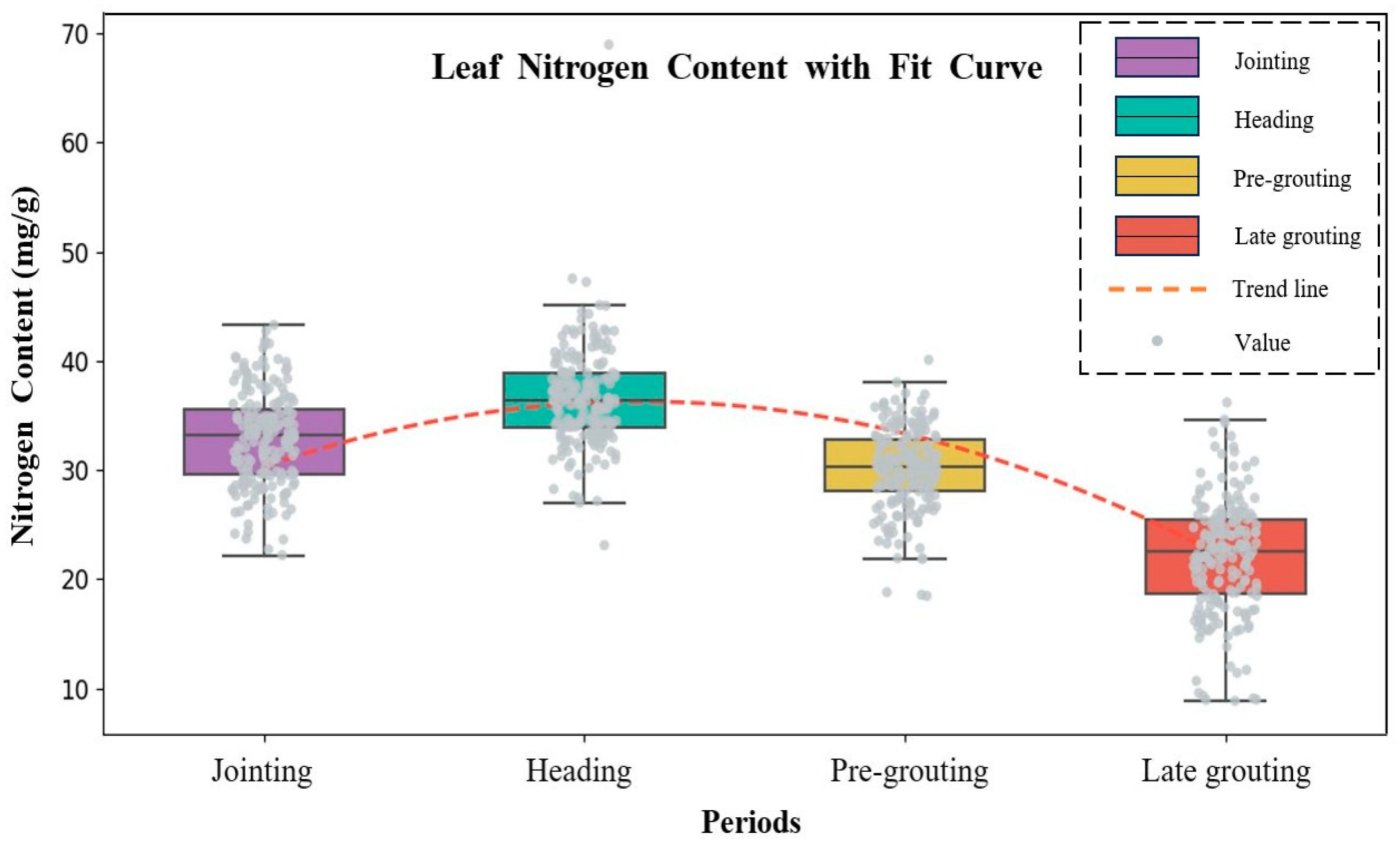
3.2. Analysis of Nitrogen Content in Winter Wheat Leaves at Different Periods

The LNC of winter wheat exhibited a dynamic trend of initial increase followed by a subsequent decline throughout the reproductive growth period, reaching its peak at the tasseling stage, as illustrated in Figure 4. The box plots of LNC at different growth stages reflect the patterns of nitrogen uptake, distribution, and translocation in winter wheat. This dynamic change is closely related to the physiological nitrogen requirements of the plant and is further influenced by environmental conditions, management practices, and varietal differences. During the period from regreening to jointing, rising temperatures reactivate root activity, prompting the resumption of plant growth. During this phase, LNC gradually increases as root systems enhance nitrogen absorption from the soil. This uptake promotes photosynthetic organ development and the synthesis of chlorophyll, essential for plant productivity.

The maximum LNC observed at the heading stage is likely attributable to accelerated nitrogen uptake, driven by the demands of spikelet differentiation and enhanced photosynthesis. At this critical stage, a high concentration of nitrogen in the leaves is required to support vigorous metabolic activity and ensure adequate accumulation of organic matter, thereby laying the foundation for subsequent grain filling. From heading to grouting, LNC declines, primarily due to the translocation of nitrogen from vegetative organs to developing seeds. This redistribution is accompanied by a reduction in photosynthetic activity, and increased nitrogen degradation and loss in the leaves. In practical agricultural production, scientific nitrogen fertilizer management and appropriate variety selection can significantly improve nitrogen use efficiency, thereby promoting both yield enhancement and quality improvement.

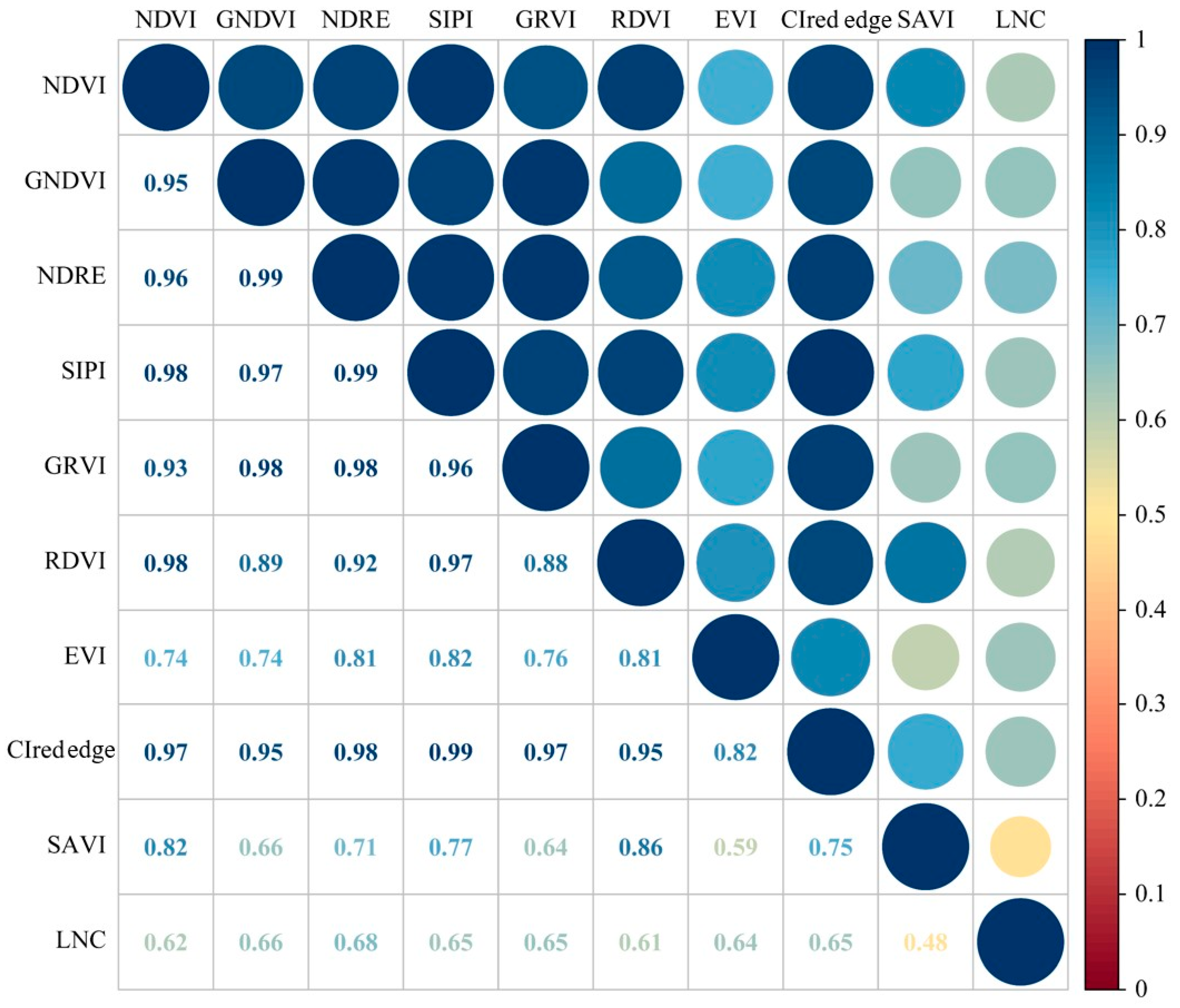
3.3. Correlation Between Vegetation Index and Nitrogen Content in Leaves

In the field of remote sensing research, vegetation indices (VIs) serve as effective indicators of surface vegetation conditions and can be used as input variables for crop growth estimation models. Analyzing the correlation between measured LNC and canopy-level vegetation indices of winter wheat provides essential data support for the accurate construction of LNC estimation models. Figure 5 is a heat map of the correlation coefficients between the nitrogen content LNC in winter wheat leaves and spectral reflectance and VIs. It can be clearly seen from the figure that LNC is correlated with vegetation index. The results showed that throughout the growth period of winter wheat, eight vegetation indices were extremely significantly correlated with the LNC value (r > 0.5). Among them, the correlation between NDRE and LNC was the highest at 0.68. The strong correlation between these VIs and LNC is primarily attributed to the direct role of nitrogen in plant growth and photosynthesis. Since the spectral reflectance properties of leaves are closely linked to their internal physiological and biochemical composition, variations in LNC affect reflectance characteristics.

Specifically, higher nitrogen content promotes chlorophyll synthesis, which in turn enhances red light absorption, reduces red reflectance, and increases near-infrared reflectance. These changes lead to higher values in vegetation indices such as the Normalized Difference Vegetation Index (NDVI). As nitrogen is a key element in chlorophyll synthesis and photosynthetic activity, the NDVI can serve as an indirect proxy for monitoring LNC variation.

3.4. Estimation of Leaf Nitrogen Content Based on Vegetation Indices

This study employs four machine learning algorithms, the RF, K-NN, SVR and RR, as well as two ensemble models, Voting and Stacking, to estimate the LNC of winter wheat based on vegetation indices. Four vegetation indices with a strong correlation to LNC were selected as feature variables for the model inputs. The estimation performance of LNC varied significantly across different models. As shown in

Table 5. Model profiles of different modeling approaches to predict nitrogen content of winter wheat leaves.

Model	Period of Fertility	R2	RMSE	MAE
SVR	Jointing	0.37	4.10	3.88
	Heading	0.48	3.34	3.02
	Pre-grouting	0.43	3.69	3.45
	Late grouting	0.33	4.25	3.94
RF	Jointing	0.58	2.97	2.76
	Heading	0.72	2.08	1.73
	Pre-grouting	0.66	2.21	1.99
	Late grouting	0.68	2.14	1.91
RR	Jointing	0.41	3.62	3.49
	Heading	0.52	3.15	3.10
	Pre-grouting	0.47	3.47	3.13
	Late grouting	0.40	3.67	3.42
K-NN	Jointing	051	3.20	3.23
	Heading	0.66	2.13	1.86
	Pre-grouting	0.65	2.19	1.98
	Late grouting	0.63	2.39	2.01
Voting	Jointing	0.69	1.98	1.80
	Heading	0.76	1.88	1.26
	Pre-grouting	0.82	1.64	1.49
	Late grouting	0.58	2.79	2.51
Stacking	Jointing	0.65	2.16	1.83
	Heading	0.73	2.05	1.77
	Pre-grouting	0.80	1.77	1.15
	Late grouting	0.71	2.18	1.94

, among the four individual machine learning models, the RF model outperformed the others, achieving the highest estimation accuracy during the heading stage (R² = 0.72, RMSE = 2.08 mg/g).

Compared to the individual machine learning models, the ensemble models (Voting and Stacking) demonstrated superior estimation accuracy. Specifically, the Voting model significantly improved the model’s generalization ability and stability, with the best results in multiple tests. Its R² value and RMSE consistently showed optimal results, and the MAE was the smallest, indicating stronger model stability, with the highest estimation accuracy in the pre-grouting stage (R² = 0.82, RMSE = 1.64 mg/g).

In comparison to individual models, Voting made full use of the advantages of RF, SVR, RR, and K-NN models, enhancing the robustness of the predictions. On the other hand, the Stacking model may have been hindered by the complexity of its meta-model, which could have overly relied on the noise predictions of base models in the training set, thus reducing its generalization ability. Moreover, Stacking’s stricter data division increases the constraints on model use. If base models generate spurious correlations due to data division biases in cross-validation, the meta-model might amplify these errors. The performance of the Stacking model heavily depends on the diversity of the base models, and if base models have highly similar predictions, the meta-model may not effectively extract additional information, potentially introducing redundancy.

In contrast, all base models in the Voting model can be independently and parallelly trained, eliminating the need for intermediate results. The final output is obtained directly through weighted voting or averaging, saving the additional overhead of training a meta-model in Stacking. Voting requires fewer constraints on base models, is more stable, and yields higher estimation accuracy, making it more suitable for this study.

To further evaluate the performance differences among the models, Taylor diagrams were plotted, as shown in Figure 6. Taylor diagrams provide a comprehensive and intuitive way to compare the statistical relationships between model predictions and observed values by simultaneously illustrating correlation coefficient, standard deviation, and root mean square error (RMSE). This graphical method offers valuable insights into the accuracy, bias, and uncertainty of model predictions. As shown in the diagram, the Voting model’s predictions are positioned at a radius of 4.5, an angle of 20 degrees, and a distance of 2.2 from the observed (Obs) point. In contrast, the Stacking model’s predictions are located at a radius of 2.8, an angle of 40 degrees, and a distance of 3.0 from the Obs point. By comparing their relative positions, it is evident that the Voting model exhibits slightly better prediction performance than the Stacking model, as it is closer to the Obs point and has a smaller angular deviation, indicating higher correlation and lower error. In comparison, the K-NN and RR models show inferior performance, with larger deviations from the Obs point, indicating lower correlation and greater prediction errors.

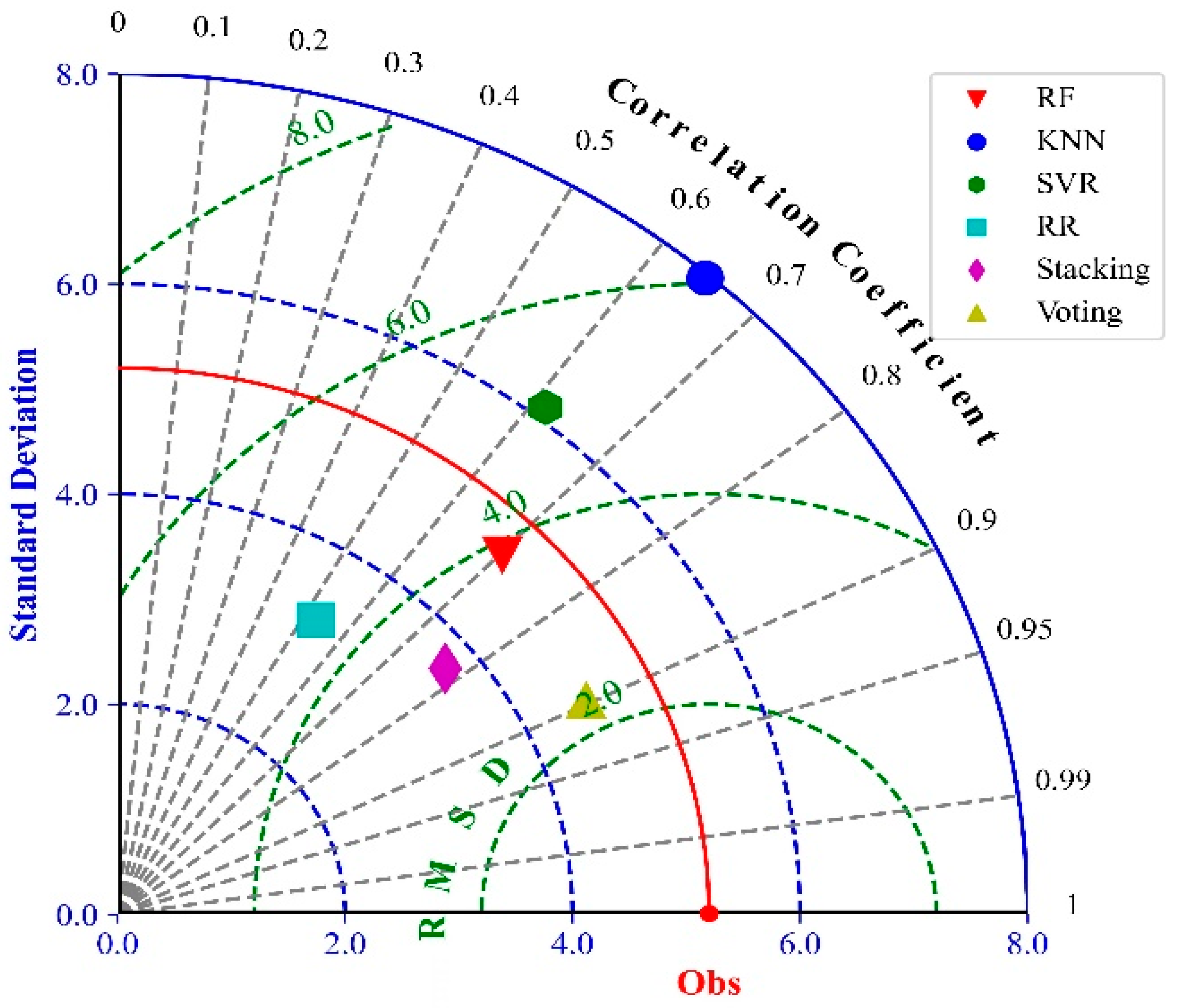
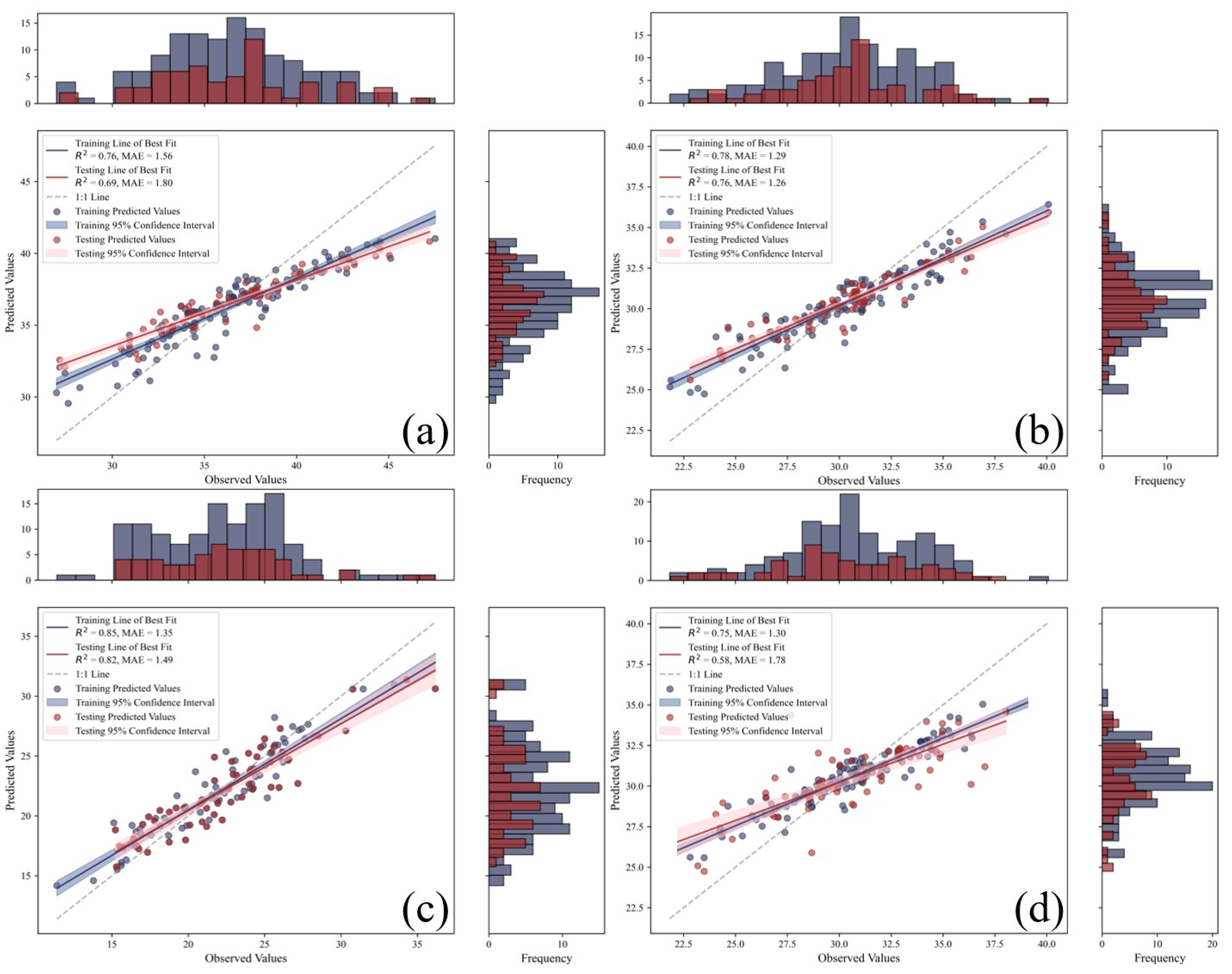
3.5. Model Construction and Inversion of Leaf Nitrogen Content Estimation Based on Vegetation Indices

This study utilized four machine learning algorithms—RF (Random Forest), SVR (Support Vector Regression), K-NN (k-Nearest Neighbors), and RR (Ridge Regression)—combined with two ensemble methods, Voting and Stacking, to build and evaluate LNC monitoring models for winter wheat at the jointing, heading, pre-grouting, and late grouting in 2023. To investigate the impact of removing soil background on model accuracy, RF-based NDVI threshold segmentation was performed for image processing, after which LNC models were constructed and estimated based on the winter wheat vegetation indices.

Based on the above analysis and the estimation results of each learning model across different growth stages, the Voting model, which demonstrated the highest estimation accuracy, was selected to construct the LNC inversion model, as illustrated in Figure 7. This figure presents the scatter plots of both the training set and the testing set for winter wheat LNC at various stages, alongside the spatial inversion maps generated from the prediction results (Figure 8).

The integrated learning models, particularly Voting, exhibited superior performance in estimating LNC. While the Stacking model improved the model’s generalization ability by combining predictions from multiple base learners (e.g., RF, RR, SVR, K-NN), the Voting model excelled in terms of model stability and error compensation, exhibiting minimal fluctuation in prediction errors. This robustness makes it especially suitable for large-scale crop monitoring applications.

The Voting-based inversion was applied to spatially map winter wheat LNC, revealing distribution patterns consistent with crop growth status. The LNC exhibited a characteristic trend of increasing initially and then decreasing, peaking at the tasseling stage. Furthermore, the average error between the model inversion results and the field measurements was less than 15%, confirming the model’s reliability and practical applicability.

4. Discussion

4.1. The Application Value of Multispectral Remote Sensing Images in Crop Canopy Segmentation

With the rapid development of UAV remote sensing technology and continuous improvements in sensor performance, dynamic monitoring of crop growth parameters has become increasingly feasible. In practical applications, visible light images provide rich spatial information that aids researchers in making accurate analytical judgments [40]. However, despite their high spatial resolution, RGB images contain only three spectral bands—red, green, and blue—which limits their ability to distinguish objects with similar colors within the visible spectrum [41]. Advancements in sensing technologies and data analysis methods have established multispectral and hyperspectral imaging as indispensable tools for continuous, non-destructive monitoring in agriculture. Multispectral images typically encompass more than four bands, enabling more effective and accurate segmentation of crop backgrounds [42].

In this study, winter wheat canopy spectral images were acquired using an unmanned aerial platform equipped with a multispectral sensor. The Random Forest algorithm demonstrated promising results in segmenting the winter wheat canopy from the background in multispectral orthophoto images. Each pixel in a multispectral image represents reflectance or radiation across multiple discrete bands, offering richer spectral information related to the chemical composition of the target object compared to visible RGB imagery, thereby enhancing segmentation performance [43]. Currently, only machine learning algorithms were employed for canopy–background segmentation. Future work could explore the integration of deep learning approaches for improved segmentation accuracy. Additionally, incorporating hyperspectral or thermal infrared data may further enhance segmentation results. Finally, evaluating the applicability of these methods across different crop types could broaden the utility of this approach in precision agriculture.

4.2. Performance Analysis of Winter Wheat Leaf Nitrogen Content Monitoring Using Vegetation Indices

Currently, the integration of UAV remote sensing imagery with vegetation indices has been increasingly applied in agricultural research. This study aims to monitor the LNC of winter wheat using UAV-based multispectral technology, thereby providing valuable data support for crop growth parameter monitoring. The results demonstrated that vegetation indices derived from multispectral images—such as the NDVI, GNDVI, and NDRE—were significantly correlated with the LNC of winter wheat, underscoring their central role in crop nutritional diagnosis. Moreover, the combined application of multiple vegetation indices improved the predictive accuracy of the models, confirming the effectiveness of using a composite vegetation index approach.

High correlations were observed between the NDVI, GNDVI, and LNC. This can be attributed to the fact that the NDVI primarily reflects chlorophyll content in vegetation, a key factor for photosynthesis. Since nitrogen is an essential element for chlorophyll synthesis, the nitrogen content in vegetation is closely related to chlorophyll concentration [44]. Additionally, NDVI is calculated from reflectance in the near-infrared (NIR) and red (RED) bands. Nitrogen-sufficient vegetation exhibits higher reflectance in the NIR band and lower reflectance in the RED band, which contributes to the strong correlation observed. Similarly, the GNDVI, which utilizes the green band, is sensitive to chlorophyll absorption. The green band’s reflectance decreases with increasing chlorophyll, enabling the GNDVI to more directly reflect nitrogen status [45]. Nitrogen-rich vegetation typically shows lower reflectance in the green band and higher reflectance in the NIR band, thus changes in these indices can effectively indicate variations in LNC over different growth periods.

The highest prediction accuracy for LNC was observed during the tasseling stage, likely due to the optimal growth condition of winter wheat at this stage, when related monitoring indices peak, thereby enhancing model performance [46]. In this study, vegetation indices were used as input variables in machine learning models to estimate LNC in winter wheat. Future research could explore the integration of deep learning approaches, such as back-propagation neural networks (BPNNs) and convolutional neural networks (CNNs), to monitor and analyze other phenological traits of winter wheat, including canopy nitrogen content (CNC) and aboveground nitrogen accumulation (PNA). Comparative studies between these models could further improve the accuracy and robustness of nitrogen content estimation in winter wheat.

4.3. Advantages of Estimating Nitrogen Content of Winter Wheat Leaves Based on Integrated Learning Models

The accuracy of winter wheat LNC monitoring models varied significantly across different modeling methods. In this study, four vegetation indices with strong correlations to LNC were selected from nine candidate indices. A monitoring and inversion model for winter wheat LNC was constructed using the Voting ensemble learning model, and a visual inversion map was generated. The results indicated that the Voting ensemble model could monitor and invert LNC more accurately compared to single models.

This superior performance may be attributed to the Voting model’s ability to effectively compensate for prediction errors through weighted averaging or soft voting strategies. In the initial settings of the model, we default that the weight of each base learner is 1. In actual prediction, in the early growth stage, Random Forest (RF) has a higher contribution because it has a strong ability to handle complex high-dimensional data and robustness in predicting nonlinear relationships. However, the integration feature of the voting model allows other basic learners, such as SVR, K-NN, and RR, to contribute effectively, especially in scenarios where their respective advantages can be utilized (for example, the performance of SVR in the linear stage and the performance of K-NN in capturing local patterns). Furthermore, when dealing with the model, we have optimized the weight distribution to ensure that no single model dominates the prediction, thereby enhancing the generalization ability and stability of the model. Particularly in complex agricultural environments characterized by large variations in light conditions, soil properties, and management practices, the Voting model demonstrates greater robustness in handling outliers [47]. By combining the predictions of multiple base models, it mitigates the prediction bias that may arise in individual algorithms due to feature limitations or noise interference [48]. Furthermore, the Voting model exhibits smaller fluctuations in error across multiple cross-validation runs, indicating enhanced stability to varying data distributions.

However, it is important to note that the model’s performance showed a decrease during the later stage of grouting, with an R² value of 0.58. This reduction in accuracy could be attributed to spectral signal attenuation caused by leaf blade aging, which impacts the reflectance characteristics of the vegetation indices. As the plant matures, the chlorophyll content and leaf structure change, leading to reduced sensitivity of certain spectral bands to nitrogen content. Additionally, as the plant enters the later stages of development, factors like canopy density and shading may also contribute to the decrease in spectral signal quality, further complicating the model’s predictions.

To address this issue and improve model performance during the later growth stages, future studies could focus on incorporating time-series data that captures the dynamic changes in spectral properties throughout the entire growth cycle. Adjusting the model to account for leaf age-related spectral attenuation could enhance its robustness and accuracy. Furthermore, integrating other complementary remote sensing data, such as thermal or LiDAR data, could provide additional information to better capture plant health and nitrogen content during the later stages of grouting.

This study confirms that the Voting model exhibits high prediction accuracy for winter wheat LNC across different varieties and growth conditions. Accurate nitrogen estimation is critical for minimizing environmental pollution and economic losses associated with the over- or under-application of nitrogen fertilizers [49].

Winter wheat LNC estimation relies on various vegetation indices as inputs. The Voting model excels in handling high-dimensional and multi-feature datasets, flexibly integrating multispectral indices. It effectively leverages the sensitivity of these indices while avoiding feature redundancy and overfitting issues common to single models, thereby improving overall model performance. Consequently, the Voting ensemble model is both efficient and reliable, meeting the demands of real-time and precise nitrogen monitoring in precision agriculture. It provides rapid predictions and offers a scientific basis for farm managers to optimize fertilization strategies.

4.4. Feasibility and Limitations of UAV-Based Multispectral Estimation for Winter Wheat LNC

As shown in

Table 6. Comparison of drone multispectral methods and traditional manual sampling methods.

Project/Indicator	UAV-Based Multispectral Method	Traditional Manual Sampling Method
Platform and sensors	DJI Phantom 4 Pro + RedEdge-MX	Manual sampling + laboratory chemical element analysis
Single job duration (this study area)	5 min	5–6 days
Data acquisition cost (estimated)	150,000 RMB (unrestricted use)	4000 RMB (single-use cost in this study, including sampling, labor, reagents, and elemental analysis)
Spatial resolution	8 cm/pixel	None
Sampling method	Non-destructive sampling	Destructive sampling
Testing frequency	Every 7 days or more frequently	Long sampling and elemental analysis cycle
Data analysis and processing	Model-based prediction with near real-time output	Laboratory testing with longer turnaround time
Applicability	Scalable to large areas, multiple time points, and different regions	Limited to small-scale or controlled experiments

, compared with traditional manual sampling methods, the use of UAV multispectral imaging for monitoring winter wheat LNC offers significant advantages in terms of data acquisition efficiency and operational costs. The data obtained through this method were representative, supports non-destructive, high-frequency data acquisition, and possesses near-real-time modeling and prediction capabilities. Although the initial equipment investment is high, it can be used multiple times, and in large-scale agricultural applications, its long-term cost per unit area is significantly lower, offering better cost-effectiveness. The above advantages indicate that this method has high feasibility and promotional value for application in precise fertilization management of winter wheat.

However, this method still has some limitations in practical application. First, the accuracy of nitrogen estimation is easily affected by external environmental factors, such as changes in light intensity, cloud cover, and wind speed during flight [50]. Second, the spatial heterogeneity of soil properties and crop growth within the sample plot may affect the model’s generalization ability [51]. Additionally, the spatial resolution of sensors currently mounted on drones is still limited, potentially making it difficult to capture fine-scale changes such as nitrogen differences within ridges, especially during the early growth stages of crops [52]. For future research, it would be worthwhile to focus on employing more advanced image segmentation techniques, such as deep learning-based methods and image super-resolution reconstruction, to enable precise segmentation of large-scale, high-volume image datasets. This approach could help develop more accurate canopy segmentation models while effectively balancing processing time and efficiency.

Therefore, subsequent studies may consider integrating multi-temporal remote sensing data, using higher-resolution sensors, and introducing robust adaptive correction algorithms for unevenly lit images, while increasing the diversity of test areas to enhance the applicability, stability, and generalis ability of the model.

5. Research Significance and Application Prospects

In this study by combining UAV multispectral images with an ensemble learning model, significantly improved the accuracy and stability of nitrogen content estimation in winter wheat leaves, providing important technical support for promoting precision agriculture. In the future, datasets of different years and different climate zones can be added. Through the integration of multi-temporal images, multi-source data and deep learning algorithms, a more comprehensive, robust, more migratory and universal nitrogen diagnosis model for farmland can be established. The proposed nitrogen estimation method based on unmanned aerial vehicle multispectral data and comprehensive learning provides an efficient and economical solution for precision agriculture. It provides a scientific basis for optimizing nitrogen fertilizer application and formulating crop management strategies, offers certain technical support for crop breeding, and has the potential for wide application and promotion.

References

1. Yi, F.; Lyu, S.; Yang, L. More Power Generation, More Wheat Losses? Evidence from Wheat Productivity in North China. Environ. Resour. Econ. 2024, 87, 907–931. [Google Scholar] [CrossRef]
2. Duan, B.; Fang, S.; Zhu, R.; Wu, X.; Wang, S.; Gong, Y.; Peng, Y. Remote estimation of rice yield with unmanned aerial vehicle (UAV) data and spectral mixture analysis. Front. Plant Sci. 2019, 10, 204. [Google Scholar] [CrossRef] [PubMed]
3. Mgendi, G. Unlocking the potential of precision agriculture for sustainable farming. Discov. Agric. 2024, 2, 87. [Google Scholar] [CrossRef]
4. ul Ain, N. Nitrogen Fertilization Strategies for Sustainable Winter Wheat Production in a Growing World. Int. J. Agric. Sustain. Dev. 2024, 6, 15–28. [Google Scholar]
5. Xue, H.; Liu, J.; Oo, S.; Patterson, C.; Liu, W.; Li, Q.; Wang, G.; Li, L.; Zhang, Z.; Pan, X. Differential responses of wheat (Triticum aestivum L.) and cotton (Gossypium hirsutum L.) to nitrogen deficiency in the root morpho-physiological characteristics and potential microRNA-mediated mechanisms. Front. Plant Sci. 2022, 13, 928229. [Google Scholar] [CrossRef]
6. Ali, A.; Jabeen, N.; Farruhbek, R.; Chachar, Z.; Laghari, A.A.; Chachar, S.; Ahmed, N.; Ahmed, S.; Yang, Z. Enhancing nitrogen use efficiency in agriculture by integrating agronomic practices and genetic advances. Front. Plant Sci. 2025, 16, 1543714. [Google Scholar] [CrossRef]
7. Anas, M.; Liao, F.; Verma, K.K.; Sarwar, M.A.; Mahmood, A.; Chen, Z.-L.; Li, Q.; Zeng, X.-P.; Liu, Y.; Li, Y.-R. Fate of nitrogen in agriculture and environment: Agronomic, eco-physiological and molecular approaches to improve nitrogen use efficiency. Biol. Res. 2020, 53, 47. [Google Scholar] [CrossRef]
8. Peron-Danaher, R.; Russell, B.; Cotrozzi, L.; Mohammadi, M.; Couture, J.J. Incorporating multi-scale, spectrally detected nitrogen concentrations into assessing nitrogen use efficiency for winter wheat breeding populations. Remote Sens. 2021, 13, 3991. [Google Scholar] [CrossRef]
9. Hansen, P.; Schjoerring, J. Reflectance measurement of canopy biomass and nitrogen status in wheat crops using normalized difference vegetation indices and partial least squares regression. Remote Sens. Environ. 2003, 86, 542–553. [Google Scholar] [CrossRef]
10. Li, D.; Chen, J.M.; Yan, Y.; Zheng, H.; Yao, X.; Zhu, Y.; Cao, W.; Cheng, T. Estimating leaf nitrogen content by coupling a nitrogen allocation model with canopy reflectance. Remote Sens. Environ. 2022, 283, 113314. [Google Scholar] [CrossRef]
11. Schlemmer, M.; Gitelson, A.; Schepers, J.; Ferguson, R.; Peng, Y.; Shanahan, J.; Rundquist, D. Remote estimation of nitrogen and chlorophyll contents in maize at leaf and canopy levels. Int. J. Appl. Earth Obs. Geoinf. 2013, 25, 47–54. [Google Scholar] [CrossRef]
12. Omia, E.; Bae, H.; Park, E.; Kim, M.S.; Baek, I.; Kabenge, I.; Cho, B.-K. Remote sensing in field crop monitoring: A comprehensive review of sensor systems, data analyses and recent advances. Remote Sens. 2023, 15, 354. [Google Scholar] [CrossRef]
13. Jiang, J.; Wu, Y.; Liu, Q.; Liu, Y.; Cao, Q.; Tian, Y.; Zhu, Y.; Cao, W.; Liu, X. Developing an efficiency and energy-saving nitrogen management strategy for winter wheat based on the UAV multispectral imagery and machine learning algorithm. Precis. Agric. 2023, 24, 2019–2043. [Google Scholar] [CrossRef]
14. Zhang, H.; Wang, L.; Tian, T.; Yin, J. A review of unmanned aerial vehicle low-altitude remote sensing (UAV-LARS) use in agricultural monitoring in China. Remote Sens. 2021, 13, 1221. [Google Scholar] [CrossRef]
15. Silva, D.C.; Madari, B.E.; Carvalho, M.d.C.S.; Ferreira, M.E. Optimizing nitrogen estimates in common bean canopies throughout key growth stages via spectral and textural data from unmanned aerial vehicle multispectral imagery. Eur. J. Agron. 2025, 169, 127697. [Google Scholar] [CrossRef]
16. Peng, X.; Chen, D.; Zhou, Z.; Zhang, Z.; Xu, C.; Zha, Q.; Wang, F.; Hu, X. Prediction of the nitrogen, phosphorus and potassium contents in grape leaves at different growth stages based on UAV multispectral remote sensing. Remote Sens. 2022, 14, 2659. [Google Scholar] [CrossRef]
17. Severtson, D.; Callow, N.; Flower, K.; Neuhaus, A.; Olejnik, M.; Nansen, C. Unmanned aerial vehicle canopy reflectance data detects potassium deficiency and green peach aphid susceptibility in canola. Precis. Agric. 2016, 17, 659–677. [Google Scholar] [CrossRef]
18. Zhu, S.; Cui, N.; Zhou, J.; Xue, J.; Wang, Z.; Wu, Z.; Wang, M.; Deng, Q. Digital mapping of root-zone soil moisture using UAV-based multispectral data in a kiwifruit orchard of northwest China. Remote Sens. 2023, 15, 646. [Google Scholar] [CrossRef]
19. Xia, F.; Quan, L.; Lou, Z.; Sun, D.; Li, H.; Lv, X. Identification and comprehensive evaluation of resistant weeds using unmanned aerial vehicle-based multispectral imagery. Front. Plant Sci. 2022, 13, 938604. [Google Scholar] [CrossRef]
20. Wang, L.; Chen, S.; Li, D.; Wang, C.; Jiang, H.; Zheng, Q.; Peng, Z. Estimation of paddy rice nitrogen content and accumulation both at leaf and plant levels from UAV hyperspectral imagery. Remote Sens. 2021, 13, 2956. [Google Scholar] [CrossRef]
21. Chlingaryan, A.; Sukkarieh, S.; Whelan, B. Machine learning approaches for crop yield prediction and nitrogen status estimation in precision agriculture: A review. Comput. Electron. Agric. 2018, 151, 61–69. [Google Scholar] [CrossRef]
22. Bharadiya, J.P.; Tzenios, N.T.; Reddy, M. Forecasting of crop yield using remote sensing data, agrarian factors and machine learning approaches. J. Eng. Res. Rep. 2023, 24, 29–44. [Google Scholar] [CrossRef]
23. Mayer, S.; van Herwijnen, A.; Techel, F.; Schweizer, J. A random forest model to assess snow instability from simulated snow stratigraphy. Cryosphere 2022, 16, 4593–4615. [Google Scholar] [CrossRef]
24. Sakamoto, T.; Sprague, D.S.; Okamoto, K.; Ishitsuka, N. Semi-automatic classification method for mapping the rice-planted areas of Japan using multi-temporal Landsat images. Remote Sens. Appl. Soc. Environ. 2018, 10, 7–17. [Google Scholar] [CrossRef]
25. Meng, Z.; Yongnian, Z. Mapping paddy fields of Dongting Lake area by fusing Landsat and MODIS data. Trans. Chin. Soc. Agric. Eng. 2015, 31. [Google Scholar]
26. Hu, H.; Bai, Y.-L.; Yang, L.-P.; Lu, Y.-L.; Wang, L.; Wang, H.; Wang, Z.-Y. Diagnosis of nitrogen nutrition in winter wheat (Triticum aestivum) via SPAD-502 and GreenSeeker. Chin. J. Eco-Agric. 2010, 18, 748–752. [Google Scholar] [CrossRef]
27. Ali, M.; Al-Ani, A.; Eamus, D.; Tan, D.K. Leaf nitrogen determination using non-destructive techniques–A review. J. Plant Nutr. 2017, 40, 928–953. [Google Scholar] [CrossRef]
28. Feng, H.; Li, Y.; Wu, F.; Zou, X. Estimating winter wheat nitrogen content using spad and hyperspectral vegetation indices with machine learning. Trans. Chin. Soc. Agric. Eng 2024, 40, 227–237. [Google Scholar]
29. Deng, L.; Mao, Z.; Li, X.; Hu, Z.; Duan, F.; Yan, Y. UAV-based multispectral remote sensing for precision agriculture: A comparison between different cameras. ISPRS J. Photogramm. Remote Sens. 2018, 146, 124–136. [Google Scholar] [CrossRef]
30. He, X.; Cai, Q.; Zou, X.; Li, H.; Feng, X.; Yin, W.; Qian, Y. Multi-modal late fusion rice seed variety classification based on an improved voting method. Agriculture 2023, 13, 597. [Google Scholar] [CrossRef]
31. Burgos-Artizzu, X.P.; Ribeiro, A.; Guijarro, M.; Pajares, G. Real-time image processing for crop/weed discrimination in maize fields. Comput. Electron. Agric. 2011, 75, 337–346. [Google Scholar] [CrossRef]
32. Chen, B.; Gu, S.; Huang, G.; Lu, X.; Chang, W.; Wang, G.; Guo, X. Improved estimation of nitrogen use efficiency in maize from the fusion of UAV multispectral imagery and LiDAR point cloud. Eur. J. Agron. 2025, 168, 127666. [Google Scholar] [CrossRef]
33. Nyengere, J.; Okamoto, Y.; Funakawa, S.; Shinjo, H. Analysis of spatial heterogeneity of soil physicochemical properties in northern Malawi. Geoderma Reg. 2023, 35, e00733. [Google Scholar] [CrossRef]
34. Adeluyi, O.; Harris, A.; Foster, T.; Clay, G.D. Exploiting centimetre resolution of drone-mounted sensors for estimating mid-late season above ground biomass in rice. Eur. J. Agron. 2022, 132, 126411. [Google Scholar] [CrossRef]
35. Rouse, J.W., Jr.; Haas, R.H.; Deering, D.W. Monitoring the Vernal Advancement and Retrogradation (Green Wave Effect) of Natural Vegetation. 1974. Available online: https://search.worldcat.org/title/Monitoring-the-vernal-advancement-and-retrogradation-(greenwave-effect)-of-natural-vegetation/oclc/67660194 (accessed on 4 May 2025).
36. Tucker, C.J. Red and photographic infrared linear combinations for monitoring vegetation. Remote Sens. Environ. 1979, 8, 127–150. [Google Scholar] [CrossRef]
37. Huete, A.R. A soil-adjusted vegetation index (SAVI). Remote Sens. Environ. 1988, 25, 295–309. [Google Scholar] [CrossRef]
38. Gitelson, A.A. Wide dynamic range vegetation index for remote quantification of biophysical characteristics of vegetation. J. Plant Physiol. 2004, 161, 165–173. [Google Scholar] [CrossRef]
39. Penuelas, J.; Baret, F.; Filella, I. Semi-empirical indices to assess carotenoids/chlorophyll a ratio from leaf spectral reflectance. Photos Ynthetica 1995, 31, 221–230. [Google Scholar]
40. Fitzgerald, P.B.; Huntsman, S.; Gunewardene, R. A randomized trial of low-frequency right-prefrontal-cortex transcranial magnetic stimulation as augmentation in treatment-resistant major depression. Int. J. Neuropsychopharmacol. 2006, 9, 655–666. [Google Scholar] [CrossRef]
41. Jordan, C.F. Derivation of leaf-area index from quality of light on the forest floor. Ecology 1969, 50, 663–666. [Google Scholar] [CrossRef]
42. Huete, A.; Didan, K.; Miura, T. Overview of the radiometric and biophysical performance of the MODIS vegetation indices. Remote Sens. Environ. 2002, 83, 195–213. [Google Scholar] [CrossRef]
43. Gitelson, A.A.; Gritz, Y.; Merzlyak, M.N. Relationships between leaf chlorophyll content and spectral reflectance and algorithms for non-destructive chlorophyll assessment in higher plant leaves. J. Plant Physiol. 2003, 160, 271–282. [Google Scholar] [CrossRef] [PubMed]
44. Liaw, A.; Wiener, M. Classification and regression by randomForest. R News 2002, 2, 18–22. [Google Scholar]
45. Perach, O.; Solomon, N.; Avneri, A.; Ram, O.; Abbo, S.; Herrmann, I. Integrating Sentinel-2 imagery and meteorological data to estimate leaf area index and leaf water potential, with a leave-field-out validation strategy in chickpea fields. Eur. J. Agron. 2025, 168, 127632. [Google Scholar] [CrossRef]
46. Vázquez-Veloso, A.; Caicoya, A.T.; Bravo, F.; Biber, P.; Uhl, E.; Pretzsch, H. Does machine learning outperform logistic regression in predicting individual tree mortality? Ecol. Inform. 2025, 88, 103140. [Google Scholar] [CrossRef]
47. Lee, J.; Kim, J. Developing a convenience store product recommendation system through store-based collaborative filtering. Appl. Sci. 2023, 13, 11231. [Google Scholar] [CrossRef]
48. Dietterich, T.G. Ensemble methods in machine learning. In International Workshop on Multiple Classifier Systems; Springer: Berlin/Heidelberg, Germany, 2000; pp. 1–15. [Google Scholar]
49. Dharmaratne, P.; Salgadoe, A.; Rathnayake, W.; Weerasinghe, A. Investigation of Accuracy for Rice Crop Parameters Predicted Using UAV Multispectral Imagery. Trop. Agric. Res. 2025, 36, 82–98. [Google Scholar] [CrossRef]
50. Cuaran, J.; Leon, J. Crop monitoring using unmanned aerial vehicles: A review. Agric. Rev. 2021, 42, 121–132. [Google Scholar] [CrossRef]
51. Yubin, L.; Xiaoling, D.; Guoliang, Z. Advances in diagnosis of crop diseases, pests and weeds by UAV remote sensing. Smart Agric. 2019, 1, 1. [Google Scholar]
52. Barbedo, J.G.A. Detection of nutrition deficiencies in plants using proximal images and machine learning: A review. Comput. Electron. Agric. 2019, 162, 482–492. [Google Scholar] [CrossRef]
Figure 1. Mengjiacun experimental base and experimental plot, Shanxi Agricultural University, Taigu District, China. ((a) the location of Shanxi Province; (b) the experimental site in Shanxi Province; (c), the experimental plots in study).
Agronomy 15 01621 g001
Figure 2. UAV multispectral imaging system.
Agronomy 15 01621 g002
Figure 3. Part of the binary image after canopy segmentation.
Agronomy 15 01621 g003
Figure 4. Box plot of leaf nitrogen content in winter wheat at different stages.
Agronomy 15 01621 g004
Figure 5. Correlation analysis of nitrogen in winter wheat leaves and vegetation index.
Agronomy 15 01621 g005
Figure 6. The results of the evaluation of different models.
Agronomy 15 01621 g006
Figure 7. Predicted distribution point plots of training sets at different growth periods ((a) Jointing period; (b) Heading period; (c) Pre-grouting period; (d) Late grouting period; the gray and brown colors represent the calibration set data and validation set data, respectively).
Agronomy 15 01621 g007
Figure 8. Inversion plot of leaf nitrogen content at different growth stages based on Voting model ((a) Jointing period; (b) Heading period; (c) Pre-grouting period; (d) Late grouting period).
Agronomy 15 01621 g008