A Chemometric Analysis of Soil Health Indicators Derived from Mid-Infrared Spectra

Abstract

Significant models predicting Soil Organic Carbon (SOC) and other chemical and biological indicators of soil health in an experimental farm with semi-arid Mediterranean Calcisol have been obtained by partial least squares (PLS) regression, with mid-infrared (MIR) spectra of whole soil samples used as independent variables (IVs). The dependent variables (DVs) included SOC, pH, electric conductivity, N, P₂O₅, K, Ca²⁺, Mg²⁺, Na⁺, Fe, Mn, Cu and Zn. The DVs also included free-living nematodes and microbivores, such as Rhabditids and Cephalobids, and phytoparasitics, such as Xiphinema spp. and other Dorylaimids. More importantly, an attempt was made to determine which spectral patterns allowed each dependent variable (DV) to be predicted. For this purpose, a number of statistical indices were plotted between 4000 and 450 cm⁻¹, e.g., variable importance for prediction (VIP) and beta coefficients from PLS, loading factors from principal component analysis (PCA) and correlation and determination indices. The most effective plots, however, were the “scaled subtraction spectra” (SSS) obtained by subtracting the averages of groups of spectra in order to reproduce the spectral patterns typical in soils where the values of each DV are higher, or vice versa. For instance, distinct SSS resembled the spectra of carbonate, clay, oxides and SOC, whose varying concentrations enabled the prediction of the different DVs.

1. Introduction

Infrared (IR) spectroscopy is a classical technique for the study of organic and mineral constituents of soil [1,2], although it always presents large limitations in the study of the macromolecular forms of Soil Organic Carbon (SOC), and, in general, in the case of complex mixtures, such as humic substances, producing broadband unspecific MIR profiles and the frequent overlapping of diagnostic bands [3].

The application of chemometric approaches is an effective method of obtaining quantitative information from IR spectra [4]. However, the scope of this approach is always more limited than that of other spectroscopic techniques, such as ¹³C NMR, due to the very different IR molar absorptivity of the different functional groups and their different vibrational modes, which mean that laborious multivariate calibration is required [5]. The application of multivariate approximations has recently facilitated progress in exploring the origin of the special variability in SOC. This has been achieved either by processing the IR spectrum as a whole, using statistical data treatments to extract relevant information from the spectral regions showing the greatest variability with regard to the different characteristics under study, or by analysing the semiquantitative information provided by the size of diagnostic peaks [6,7,8,9,10].

In this context, PLS regression is a widely used routine method for the indirect determination of soil physicochemical properties, often including agrochemical fertility descriptors. After calibration with a reduced set of samples, it allows the precise determination of soil properties (DVs, e.g., SOC, nitrogen (N), phosphorus (P), etc.) that would otherwise require the use of costly and time-consuming wet chemical techniques for their determination. In particular, IR partial least squares (PLS) analysis is capable of extracting both qualitative and quantitative information from soil spectra [11,12]. Nevertheless, PLS also offers great potential for basic exploratory research, such as the calculation of a series of indices across the entire wavelength domain (i.e., the spectral arrays of the IVs) that provide information on their discriminant power with respect to the DV under study. In the case of PLS, the VIPs for several DVs have often been used in the form of spectral-like plots [6]. In fact, peaks in the VIP traces reveal soil components with high predictive power (regardless of the fact that they could be causally related), which are reflected in the corresponding spectra [12,13].

In any case, although the application of chemometric models to assess the physical and chemical characteristics of soils has been the subject of numerous studies, it is less common to apply these approaches to the study of emerging soil properties. These properties depend on complex interactions between several soil constituents. This phenomenon is prevalent in systems exhibiting substantial internal functional redundancy, i.e., the capacity of a system to maintain its integrity through the redundancy of its structural and functional relationships, such as those multiple factors involved in the regulation of soil health. Among soil organisms, nematodes exhibit a number of characteristics that make them an excellent group for use in modelling soil microfauna. They are highly abundant, ubiquitous and diverse, participating in numerous soil food web links and exhibiting sensitivity to agricultural disturbance [14]. In principle, there is no reason to suppose that the survival and development of soil organisms should not be related to the variable proportion of soil constituents (nutrients, mineral fractions that can influence moisture, salinity or soil reaction, etc.) which could be directly or indirectly reflected in MIR spectra.

As demonstrated in previous studies [15,16], there is a clear indication of the capacity to correlate spectroscopic profiles within the MIR range with populations of free or phytopathogenic nematodes. Whilst the majority of these studies have concentrated on analytical aspects, they have also emphasised the potential for chemometric approaches to enhance the predictive capabilities of existing models. The potential of such multivariate methods is to extract the underlying information that arises from high-order correlations between soil characteristics, which are often reflected in the intensities of the peaks in the MIR spectra.

In the present study, a series of PLS models were initially compared in order to optimise the determination of different soil DVs, i.e., typical soil agroecological properties (SOC, macro- and micronutrients, etc.) in addition to major functional groups of soil nematodes. In all cases, the IVs, or predictor matrix, were constituted by the digital MIR spectra of whole soil samples. In a subsequent stage, following confirmation that specific soil characteristics (DVs) were significantly reflected in the MIR spectra and could be used to predict them, DVs not successfully predicted from the IR data (at least with p < 0.05) were disregarded, and attention was focused on those DVs for which the predicted vs. observed values were significantly correlated. Subsequent analysis of the MIR profiles was conducted for these models in order to identify spectral regions or individual peaks that could explain the variability of the DVs. In accordance with the aforementioned points, the objective of this study is not to merely predict soil properties using PLS applied to MIR spectra. This would only be of local interest to the soil under study, in addition to requiring a greater number of sampling points for a more accurate calibration. Consequently, this study is regarded as an exploratory investigation into the automated interpretation of spectra [17]. The approach involved the comparison and interpretation of traces of univariate and multivariate statistical indices, graphed in the wavelength domain in the range of 4000 to 450 cm⁻¹.

Despite the fact that the objective of this analysis of the MIR spectral profiles was not to postulate cause-and-effect relationships, it is evident that such an approach may be an effective method for identifying the set of soil characteristics useful for defining soil health, which are reflected in the IR spectra.

2. Materials and Methods

2.1. Experimental Field

The experimental site corresponded to a vineyard near Socuéllamos (Ciudad Real, Castilla-La Mancha, Spain, 39°20′ N, 2°47′ W). This area has a continental Mediterranean climate. The average annual temperature is 14–15 °C, with the coolest month averaging 5 °C and the warmest month 26 °C. The altitude is around 670–700 m above sea level [18]. The experimental field followed a randomised block design with three treatments applied to the soil: wine and sugar beet vinasses and no treatment. The experiment was conducted between February 2017 and October 2019. At the conclusion of the experiment, soil samples were collected with a shovel at a depth of 0–20 cm.

These experimental treatments are usual in Mediterranean areas, where biofumigation—or biodisinfestation—practices may be helpful for the control of soil-borne diseases [19]. The field study consisted of an eight-year-old vineyard of the variety “Cencibel” with a planting frame of 2.5 × 2.5 m. The farm was irrigated by sprinklers. In this farm we observed not only the presence of the virus-transmitting nematode Xiphinema index, but also a significant presence of second-stage (J2) juveniles of the root-knot nematode Meloidogyne arenaria.

The most representative soils are Petric Calcisols, which are associated with Calcaric Cambisols, both of which show accumulations of calcium carbonate in their profiles, either in the form of calcretes, nodules or pulverulent masses. In some plots there was some influence from neighbouring Calcaric Regosols [20]. As in many field experiments on semi-arid soils, the differences in nematode size populations between treatments (wine and sugar beet vinasses) were not statistically significant for the agronomic year of the experiment. However, the experimental field remained a representative mosaic of plots with considerable spatial heterogeneity in soil chemical composition and nematode population size. Consequently, the results analysis strategy was revised. Instead of assessing the effects of the treatments, the focus shifted to understanding the reasons for the observed differences in soil characteristics and the absence of potentially phytopathogenic nematodes in certain plots, which could be attributed to suppressive soil conditions.

2.2. Basic Soil Physicochemical Properties (Agrochemical DVs)

Soil samples were collected in duplicate in 2.5 × 2.5 m² field plots from the upper 10–20 cm of the topsoil (Ap horizon). Samples were collected from the soil surrounding (or canopy of) 4 vine plants in the central area of each experimental plot (12 plots in total). The soil samples were then air-dried and homogenised to 2 mm (fine earth).

The primary soil diagnostic criteria were analysed in accordance with the methodology outlined by the Soil Survey Staff [21]. Soil pH and electric conductivity (EC) were measured in water suspension (1:2.5 w:w). The SOC was determined by wet oxidation with 1N K₂Cr₂O₇ following the Walkley–Black procedure [22]. Total nitrogen (N) was determined by the Kjeldahl method [23]. The exchangeable cations (Na⁺, K⁺, Ca²⁺ and Mg²⁺) were extracted at pH = 7 with ammonium acetate [24] and analysed by atomic absorption spectroscopy, whereas total cation exchange capacity (CEC) was measured with selective ion electrodes. The extraction of soil microelements was conducted using ammonium acetate and EDTA at a pH of 4.5, as described by Lakanen and Ervio [25], and the analysis was performed using inductively coupled plasma atomic emission spectroscopy. The extraction of available phosphate followed the method outlined by Burriel and Hernando [26].

2.3. Soil Biology (Biological DVs)

The fauna of a soil is contingent on the properties and composition of the soil. The present study focused on soil nematodes within the broader context of edaphic biology. This particular fauna constitutes a component of the soil food web, and the characteristics that define its life cycle, body size and reproductive strategy render it susceptible to varying degrees of sensitivity to environmental disturbances [27].

Microbivores (Rhabditids and Cephalobids) comprise groups that feed on bacteria and fungi. The Dorylaimids represent an Order that includes a wide diversity of families (predatory and omnivorous), and their presence is indicative of soil quality [10]. However, this Order also comprises plant-feeding nematodes, such as the genus Xiphinema (Family Longidoridae) which includes several species that transmit viruses, including X. index. This species is frequently found in association with vineyards and is the primary grapevine problem due to its ability to transmit the Grapevine Fan Leaf (GFLV) virus.

Flegg’s method [28] was utilised for the extraction of nematodes from the soil, with the resulting samples being expressed as individual organisms per gram of soil. The DVs were then simplified to XIPH, DOR and RHA.

2.4. Mid-Infrared Spectroscopy (Predictors Matrix, IVs)

The MIR spectra of the entire soil samples were obtained using a benchtop instrument, the Cary 630 (Agilent, Santa Clara, CA, USA), with KBr optics and the transmission module. While the preliminary spectra obtained with the attenuated total reflectance module were perfectly valid for the routine IR analysis of the soil material, the more time-consuming technique of using KBr pellets (using 200 mg KBr dried under vacuum overnight and 3 mg soil homogenised with a planetary mill with agate balls to pass a 100 µm sieve) was selected in order to obtain extended spectral information between 600 and 350 cm⁻¹, a range where the diagnostic absorption of some clays and oxides was expected.

2.5. Data Treatments

2.5.1. Management and Pretreatment of MIR Spectra Before PLS

The digital spectra (4000–350 cm⁻¹) were exported as ASCII files comprising 1000 data points for further data processing, including PLS. In order to enhance the fittings in the PLS models and to optimise the spectral traces representing indices from uni- or multivariate data treatments, a series of spurious features in the raw MIR spectra were amended. The primary motivations for this approach were as follows: (i) the presence of background absorptions or spectral noise, necessitating additional smoothing; (ii) the inadequate spectral resolution of the resulting profiles, characterised by broad peaks; (iii) the challenges associated with sub-optimal baseline correction. In an effort to rectify these issues, four distinct strategies were employed:

(a)

The elimination of data points within the interval 2404–2363 cm⁻¹, encompassing the range in which CO₂ (an impurity derived from air) undergoes absorption (zero-filling followed by a moving average with the neighbouring baseline points).

(b)

The employment of digital smoothing through the implementation of the Savitzky–Golay algorithm. The algorithm is typically applied to spectra with n = 1000 points using a 2-point window.

(c)

The second derivative spectra were obtained in order to sharpen the peaks and minimise the differences between different spectrum at the baseline level [6].

(d)

The entire spectrum was processed with specific numeric pretreatments or transformations that are typical of chemometric studies [29]. The aforementioned treatments are outlined below: (i) Mean centring (MC), which entailed calculating the mean spectrum of the data set and subtracting it from each spectrum. (ii) The removal of baseline effects through multiplicative scatter correction (MSC), which entailed correcting the spectra to an ideal, average spectrum so that the baseline and amplification effects were at the same average level in every spectrum [30]. In models with a high degree of significance, where there are considerable differences between samples with low and high values, the impact of MSC was found to be negligible. However, MSC is recommended as it did not introduce artefacts in subtractions and was shown to enhance the quality of soil PLS models based on near- or MIR spectra [31]. (iii) With the standard normal variate (SNV) the centre of each spectrum was determined and each spectrum was scaled by its standard deviation. The resulting spectra thus possessed a mean value of 0 and a variance of 1, irrespective of the original values of the absorbance. (iv) Standard normal variates and detrending (SNV + DT), is a process which served to eliminate the multiplicative interference of scatter and particle size [32]. Each spectrum was then normalised to a mean of zero and a variance of one, followed by a detrending step. This process involved the fitting of a second-order polynomial to the SNV-transformed spectrum and the subsequent subtraction of this from the original spectrum in order to correct for wavelength-dependent scattering effects. Furthermore, the combination of the aforementioned pretreatment methods, such as SNV+MC, was also evaluated.

All of these treatments, carried out with the ParLes software [29], were used both to process the spectra before performing PLS and to obtain transformed spectra to be used to obtain correlation traces or spectral subtractions.

2.5.2. Forecasting Models

Partial least squares regression (PLS) is a generalisation of multiple linear regression (MLR) that is of particular interest because, unlike MLR, it can analyse data with strongly collinear, noisy and numerous independent variables (IVs). In general, PLS is regarded as a suitable linear multivariate model for explaining complex relationships in matrices in which the number of IVs (predictors, spectral intensities) is much larger than the number of individuals (samples), which are frequent in spectroscopic studies [33]. The PLS regression was conducted utilising the ParLeS software [29], which incorporates the aforementioned specific spectral pretreatment routines. The selection of a correct number of latent variables (LVs) for each PLS model for the different DVs (cross-validation with the leave-one-out method) was achieved by utilising the Akaike Information Criterion (AIC [34]), with the comparison of models with fully randomised DVs being the primary method of comparison. In addition, the root mean square error (RMSE) was examined for model selection, although the AIC and randomisation of the DVs were preferred as more rigorous, considering that RMSE does not adequately account for the growth of variance as a function of model complexity [35], often leading to overfitted models.

2.5.3. Extracting Information on Soil Chemistry and Biology from MIR Spectra

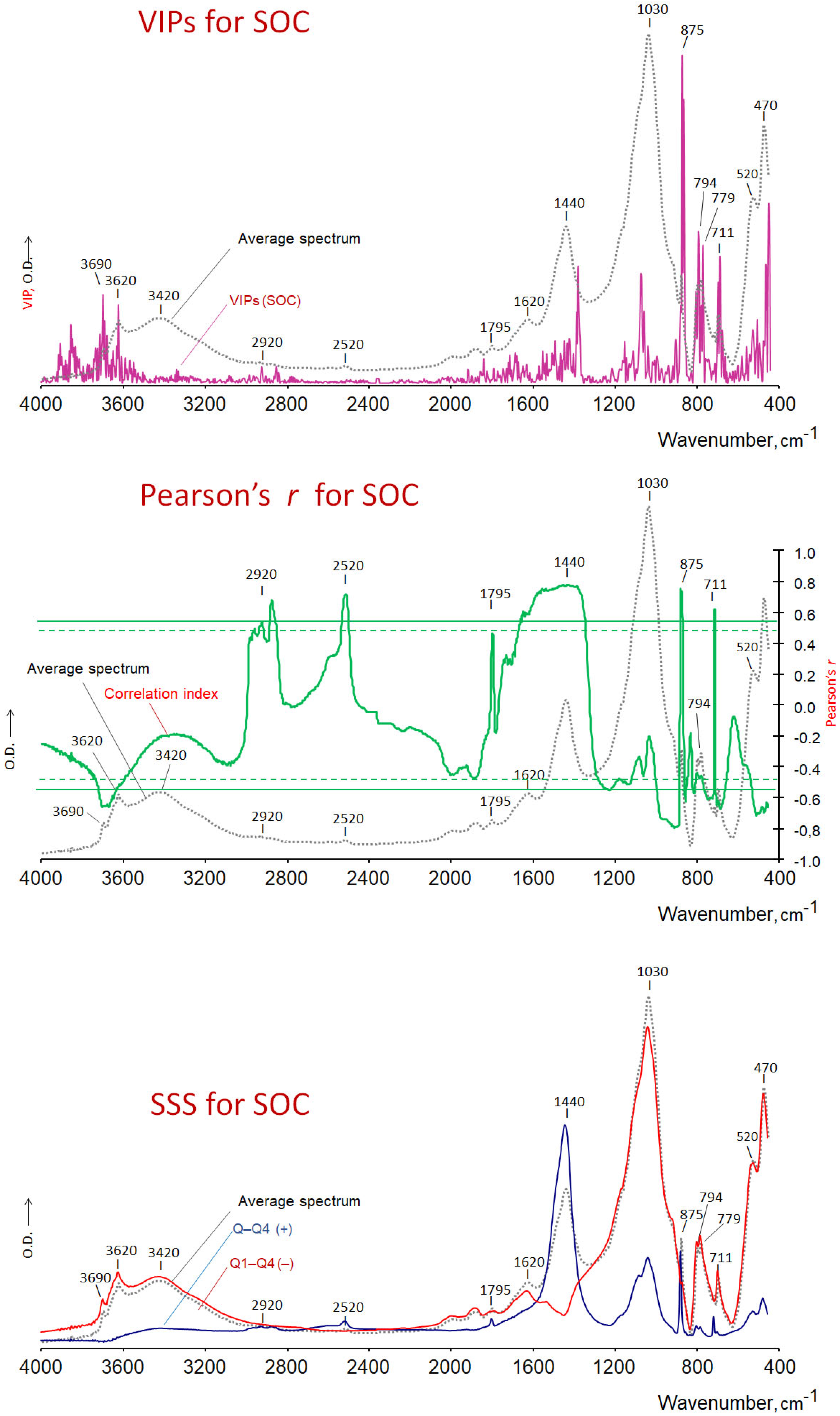
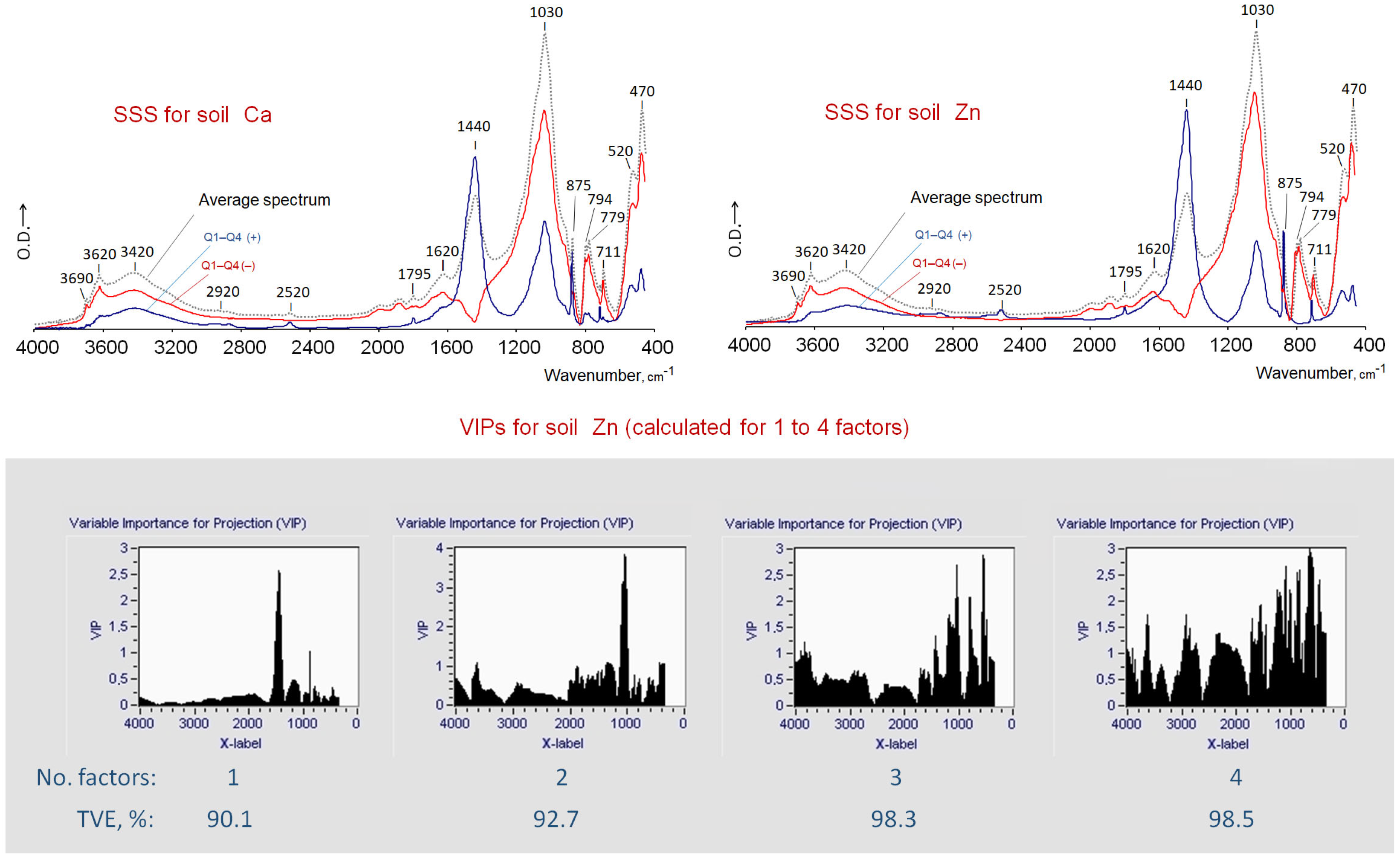
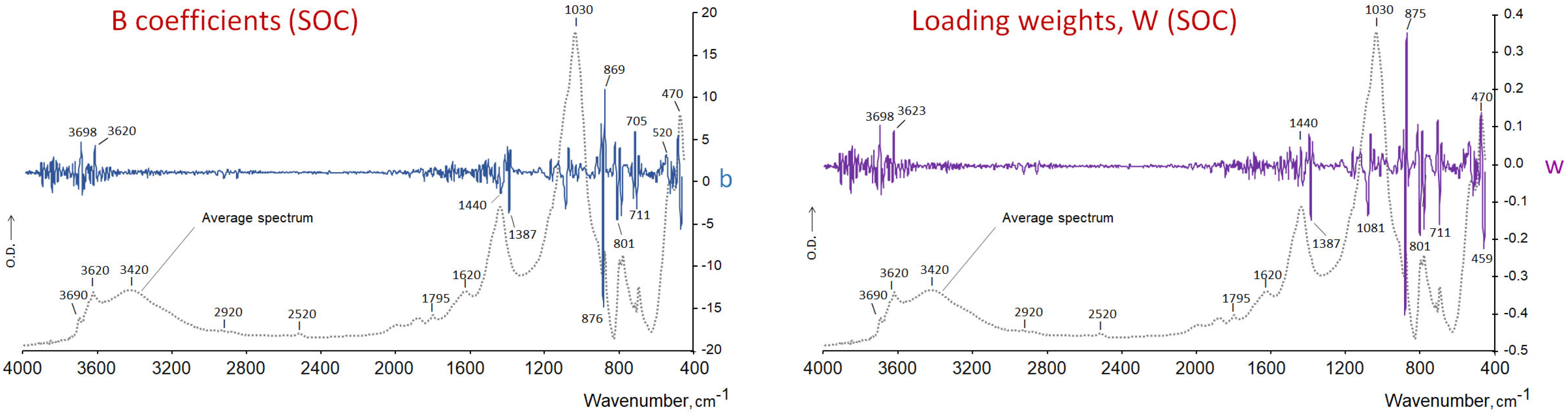
For those soil characteristics (DVs) for which the previous PLS forecasting models demonstrated significance, it could be deduced that only a limited number of soil constituents could account for the variability between different sampling points. The aforementioned constituents were contained within the FTIR spectra profiles. In order to demonstrate the spectral regions that exhibited greater predictive potential with regard to the DVs, a series of plots featuring ‘new’ or ‘derived’ spectral profiles were prepared for visual comparison. These plots represent, for each DV, indices calculated by univariate or multivariate treatments across the entire wavelength range:

(a)

The VIPs calculated for the different significant PLS (p < 0.05) models,

(b)

The factor scores of the significant PLS models.

(c)

The beta coefficients from the above PLS models (calibration equation coefficients showing the importance of spectral bands in the PLS calibration, i.e., representing the contribution of each IV to the model, with positive or negative signs [36]). The aforementioned indices were calculated with ParLes software [29].

(d)

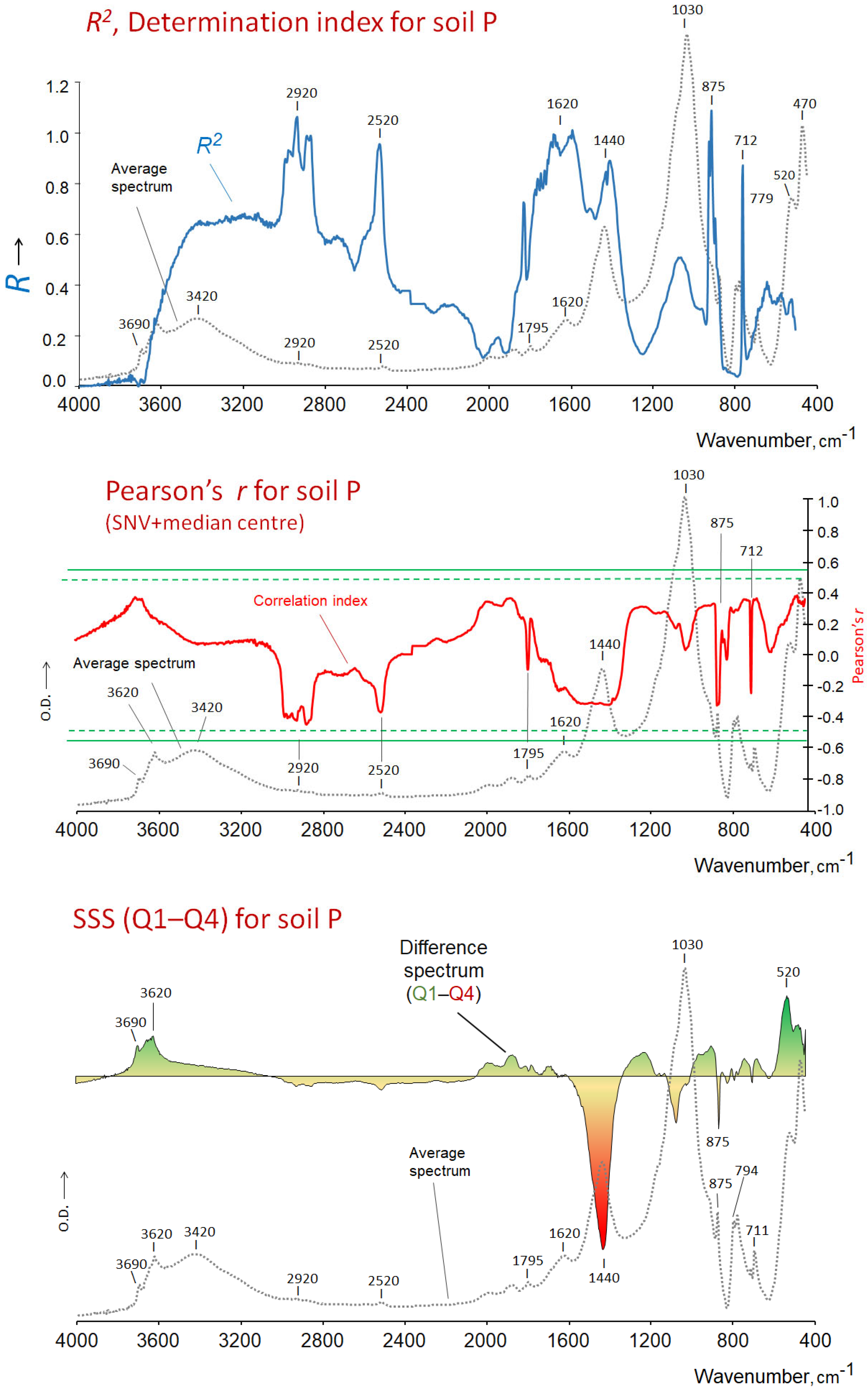
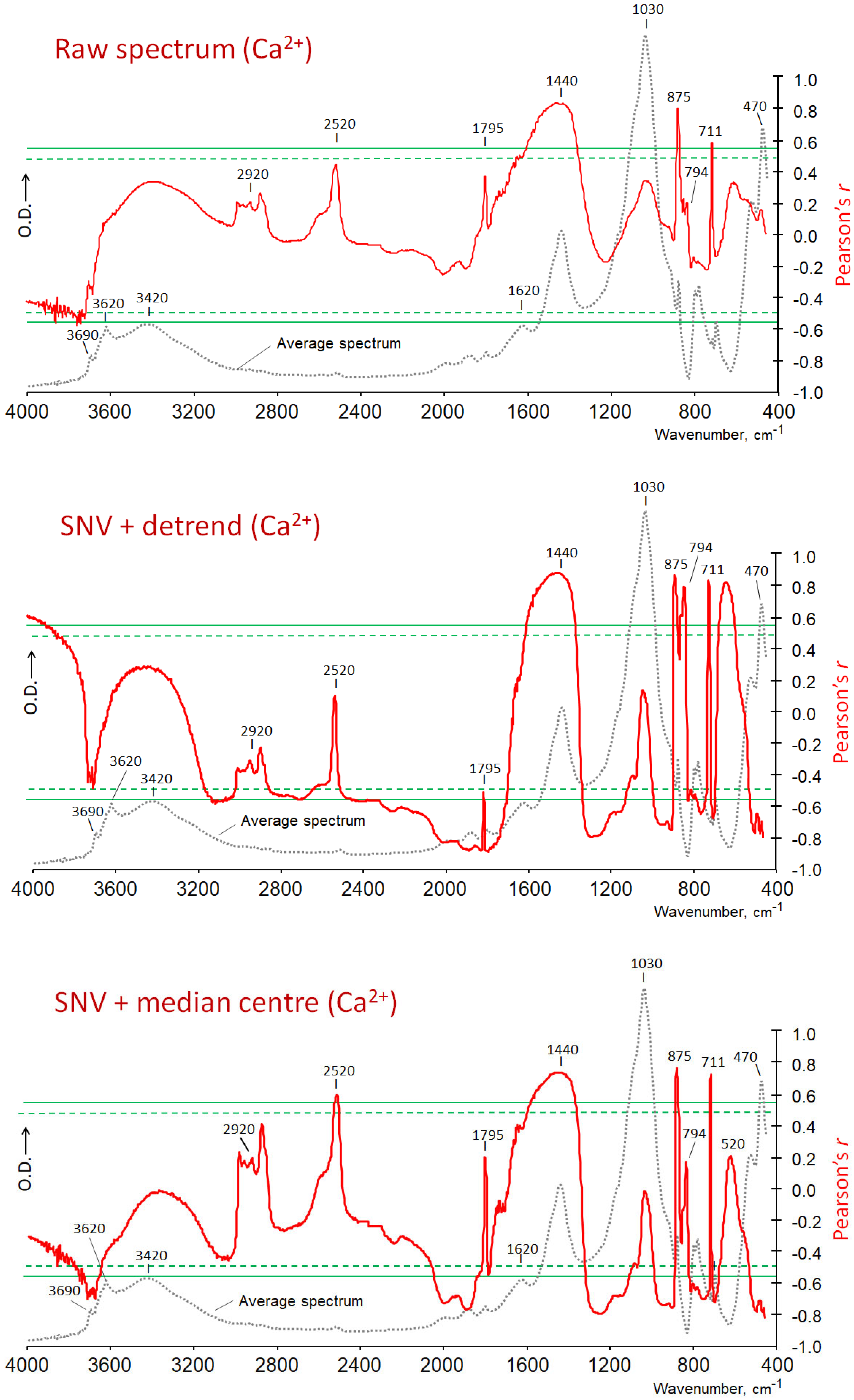
Pearson’s correlation coefficients between the whole array of spectral data points and each DV, using authors’ programs [37].

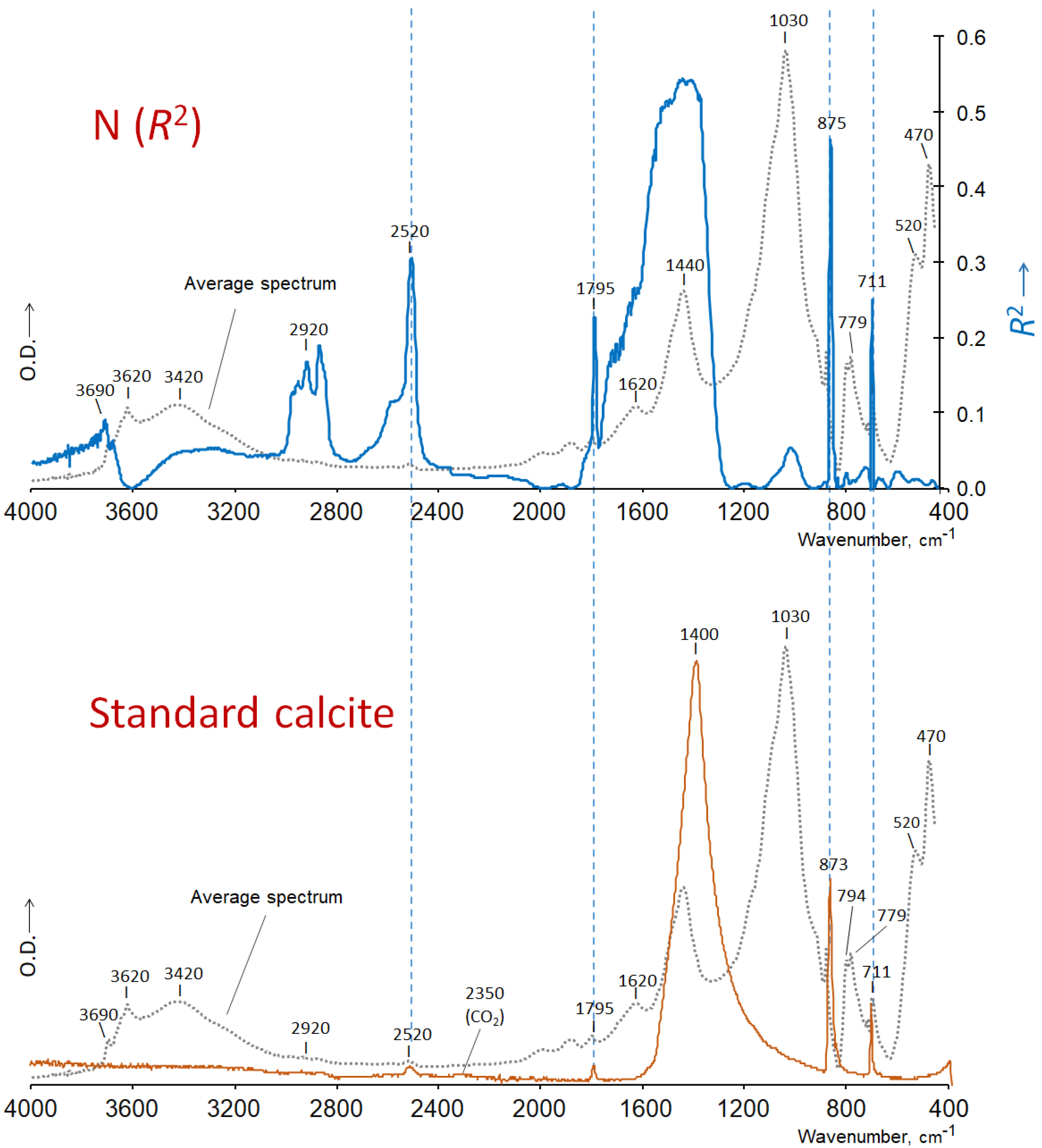
(e)

The coefficient of determination, R², i.e., the square of the correlation coefficient.

(f)

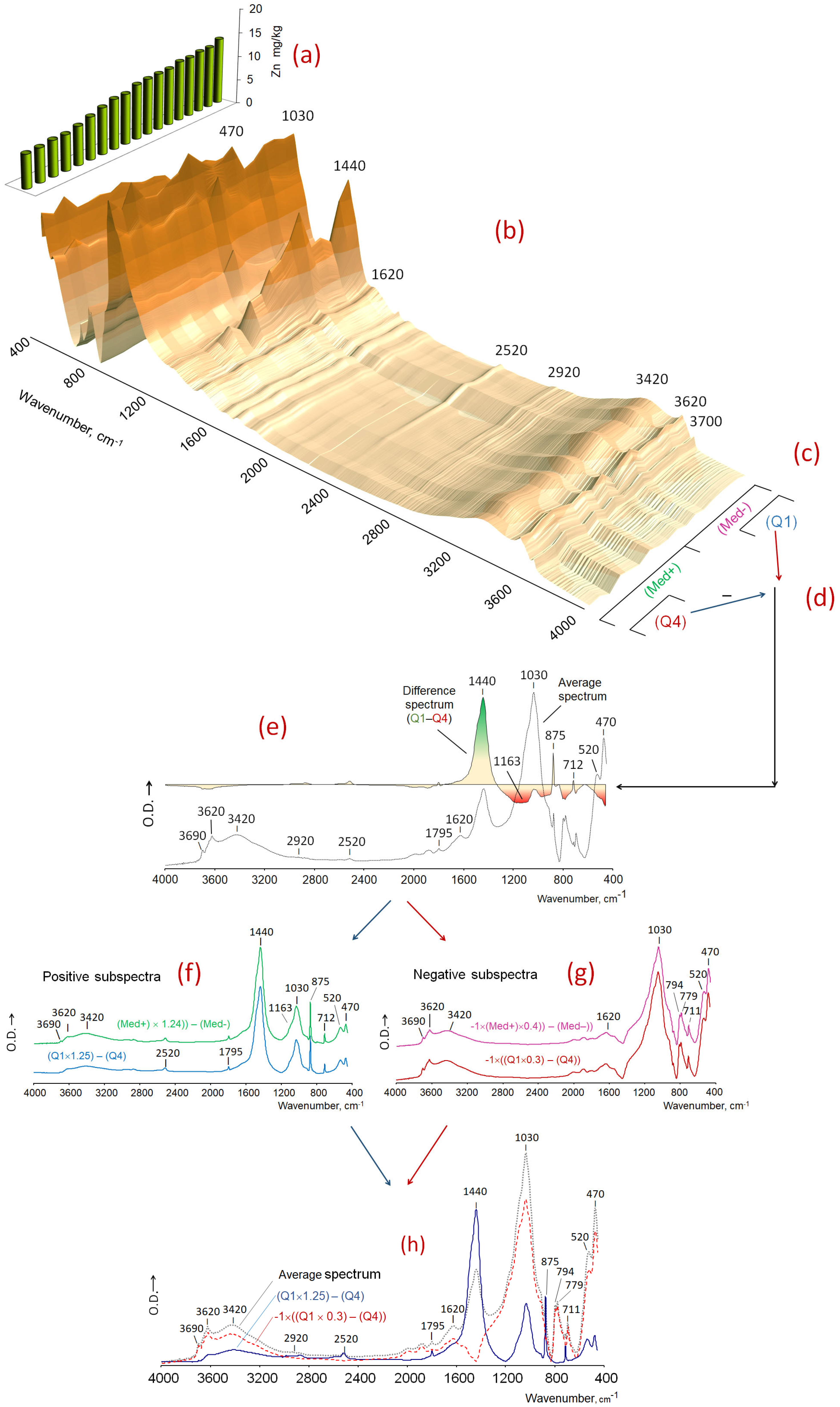
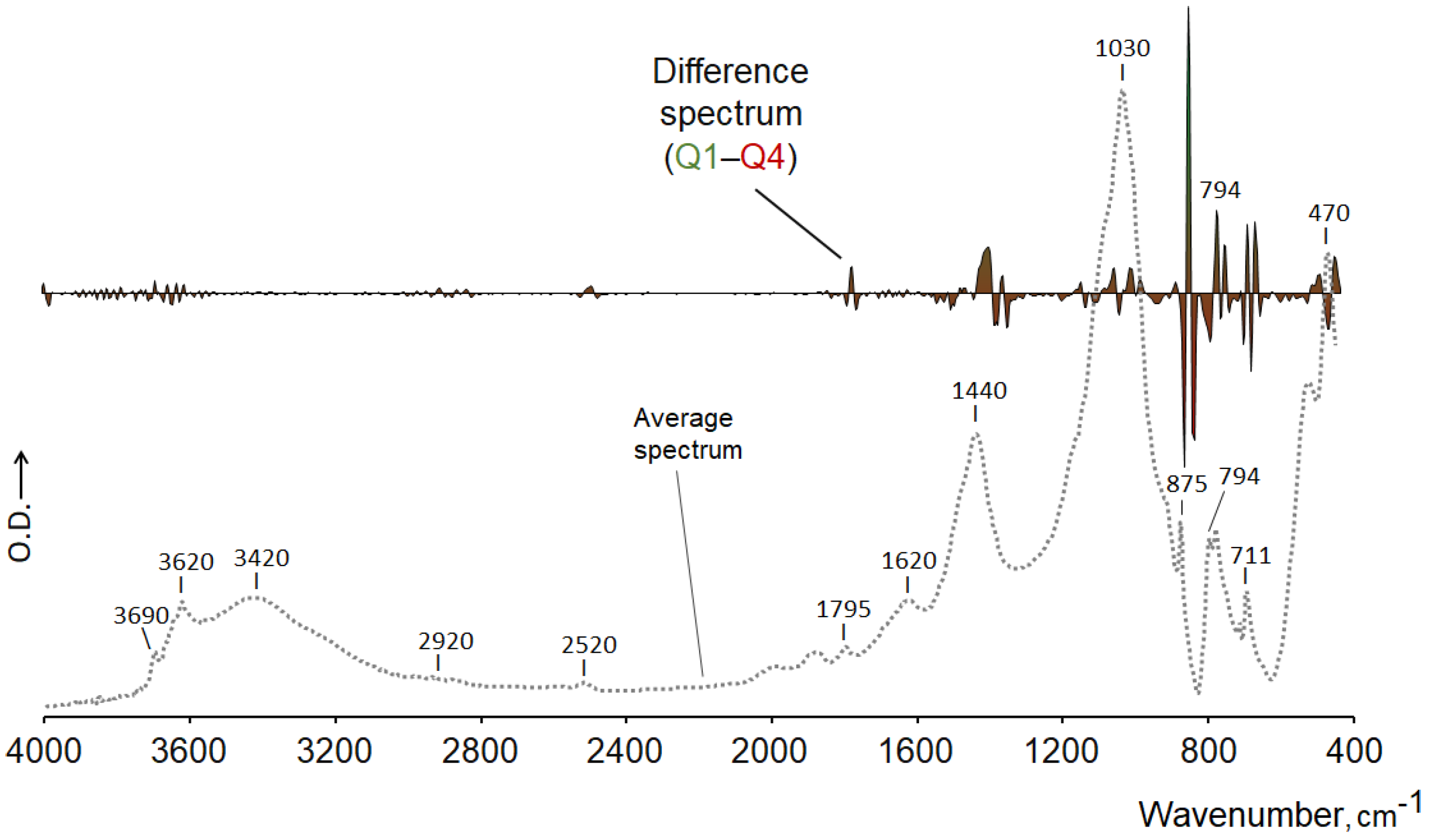
The subtracted spectra.

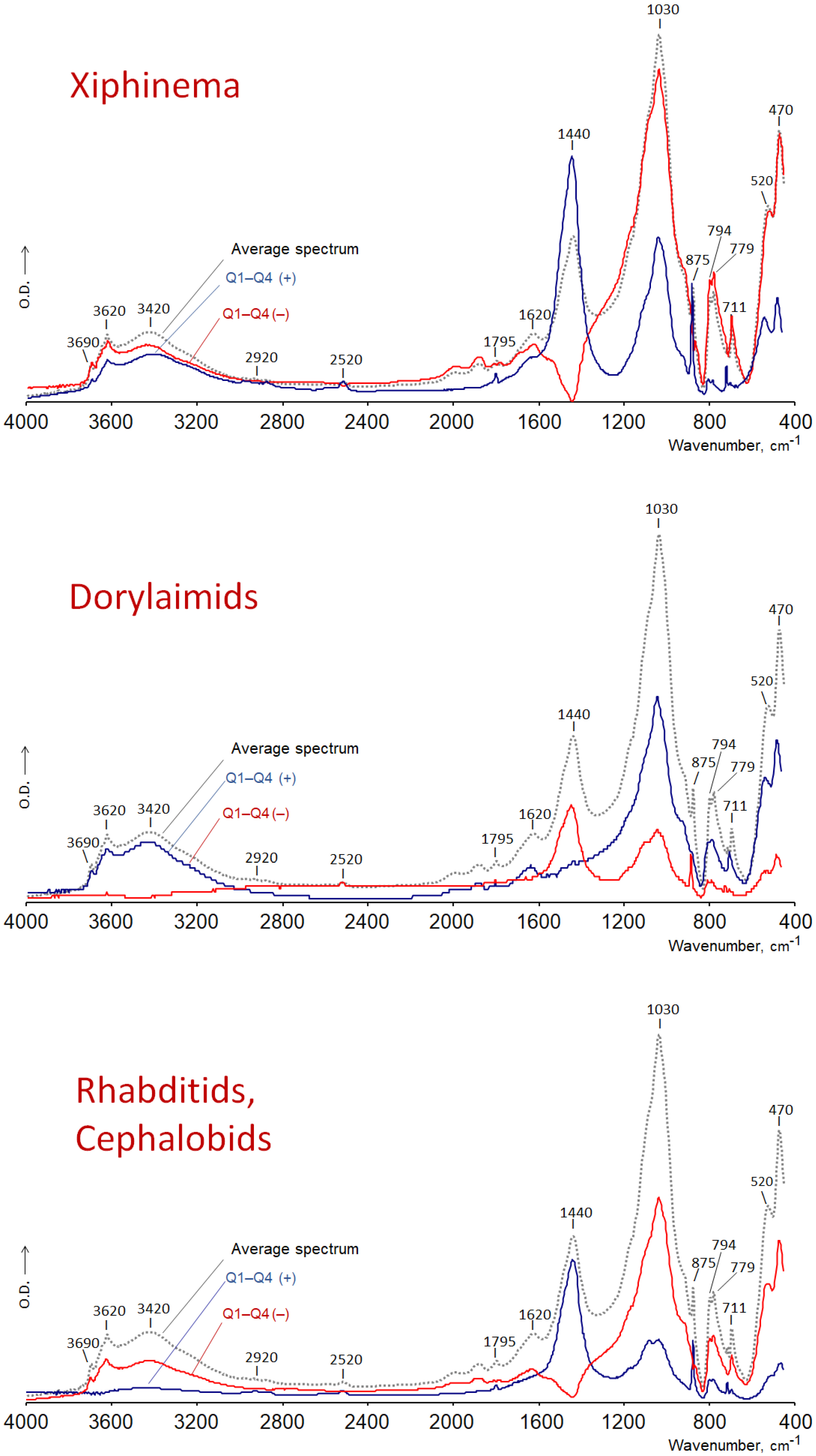
Subtracted Spectra

In addition to the aforementioned classical indices derived from univariate or multivariate data treatments, a straightforward approach is to subtract pairs of average spectra corresponding to soil samples with extreme values of a DV. In the initial comparisons, the digital subtractions were carried out between the spectrum with the lowest value of a DV and the spectrum with the highest value of the same DV. The positive and negative peaks displayed were useful for differentiating the spectral bands prevailing in samples with high levels of the given DV, and vice versa.

A more robust approach would be to subtract the mean spectra from samples exhibiting high or low values of the different DVs. This method comprises two principal stages (Figure 1a–e). Initially, the spectral data points (VIs) are normalised as total abundances, whereby the sum of all spectral intensities of each spectrum is set to a constant value (e.g., 100). Subsequently, the spectra are then ordered according to the values of the different DVs. A subset of spectra corresponding to soil samples with high DV values (e.g., above the median) and another subset of spectra corresponding to samples with low DV values are then averaged. The spectral intensities are then directly subtracted from these average spectra. The resulting plot is a trace with positive peaks, which correspond to the prevailing spectral intensities in soils with higher values of the DV, and valleys or negative peaks, which indicate higher intensities in samples with low values of the DV. The subtraction spectra (Figure 1e) are centred on the baseline (zero value) and have an integration value of zero. Two types of subtracted spectra were prepared and compared for analysis: (i) spectra from samples above and below the median of the DV; (ii) average spectra from samples in the upper quartile (Q1) of the distribution of the DV subtracted from the average spectra from samples with low values of the DV, i.e., Q4.

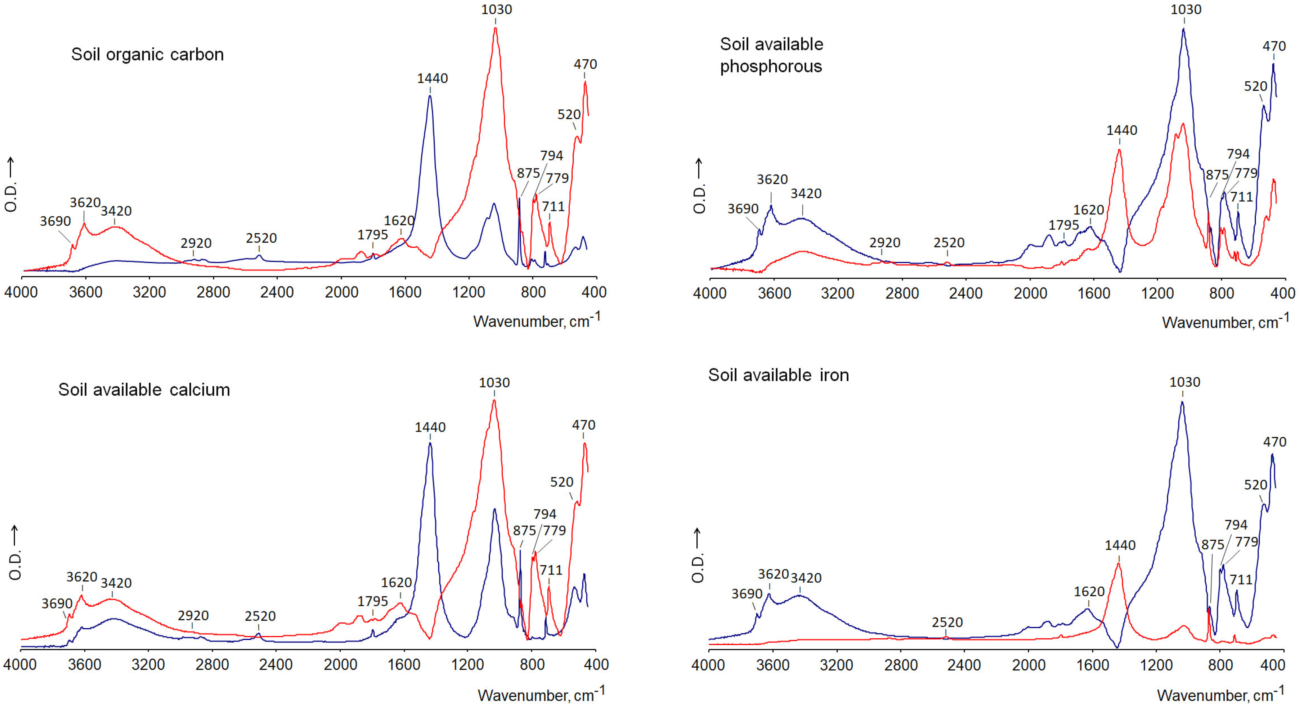
Scaled Subtraction Spectra (SSS)

In order to obtain additional perceptual plots that illustrate the spectral features characteristic of the spectra from samples with opposite levels of the DV, two independent spectral traces were obtained (Figure 1a–h). These traces, termed SSS, emphasise the positive or negative intensities in the aforementioned subtracted spectra. A positive trace is obtained by multiplying the MIR subtraction spectrum (initially with positive and negative values) by a factor that renders the difference value at the most intense valley in the subtracted spectrum equal to zero. Consequently, the subtracted array is comprised exclusively of positive values. The same operation is carried out to emphasise the spectral components responsible for the negative subtraction intensities. In this instance, the subtraction spectrum was multiplied by a factor to obtain a trace where the highest value would coincide with the virtual baseline (zero value). Consequently, all peaks in the subtraction plot are negative. The values in the resulting SSS were then multiplied by (–1) and represented as a positive value trace superimposed with the aforementioned positive trace of subtracted intensities. The combined plot (Figure 1h) comprises uncorrelated spectral traces, which, respectively, illustrate the extreme spectroscopic features of samples with high and low values of the DV. In other words, they are the virtual spectra of the soil components that are most common in the samples with the highest DV values, and of the soil components that are most common in the samples with the lowest DV values.

3. Results

3.1. Forecasting Soil Agroecological Properties (Biological and Physicochemical) by PLS

It is noteworthy that the PLS model was able to successfully predict not only SOC and the majority of the chemical variables, but also soil features such as the size of the nematode populations. These are not trivially related to the other DVs determined in the experimental plots (

Table 1. Main analytical characteristics of soil in experimental farm.

Ref.	Tre.	SOC g/kg	pH	EC mS/cm	N g/kg	P2O5 g/kg	K+ g/kg	Ca2+ g/kg	Mg2+ g/kg	Na+ g/kg	Fe mg/kg	Mn g/kg	Cu mg/kg	Zn mg/kg	Xiph	Xind	Dor	Ench	Rha
1.3	C	4.43	8.15	0.19	0.45	0.02	0.26	3.91	0.22	0.01	15.55	90.98	1.36	12.50	0	0	105	0	5
3.4	C	4.24	8.11	0.18	0.36	0.05	0.18	3.61	0.18	0.01	12.56	74.16	1.13	12.56	10	0	100	15	10
5.5	C	2.39	8.17	0.11	0.21	0.16	0.19	1.97	0.17	0.01	15.15	99.76	1.05	6.91	5	5	40	15	0
5.7	C	2.03	7.94	0.10	0.18	0.20	0.19	1.43	0.16	0.01	20.07	95.62	1.22	6.43	20	0	40	65	0
6.1	C	2.39	8.04	0.16	0.36	0.01	0.25	4.35	0.23	0.01	13.29	96.35	1.24	11.29	10	0	115	0	5
6.3	C	3.50	8.07	0.14	0.28	0.05	0.21	4.01	0.20	0.00	14.68	103.47	1.19	10.74	40	0	115	5	5
1.5	V	4.93	7.93	0.23	0.48	0.02	0.32	3.57	0.18	0.01	11.35	55.97	2.00	13.55	40	5	110	15	40
1.7	V	4.20	8.10	0.27	0.52	0.04	0.32	3.89	0.19	0.01	9.81	49.36	1.23	11.42	10	0	160	20	10
1.8	V	4.01	8.04	0.20	0.42	0.06	0.29	3.73	0.19	0.01	11.37	62.10	1.67	11.42	5	0	70	15	5
2.1	V	4.56	8.04	0.21	0.52	0.01	0.32	3.77	0.24	0.01	12.93	88.11	1.59	10.86	20	0	100	10	25
2.2	V	4.20	8.05	0.28	0.42	0.06	0.39	3.70	0.20	0.01	12.00	80.54	1.42	11.03	0	0	145	25	15
2.3	V	4.56	7.66	0.75	0.58	0.16	0.54	3.67	0.17	0.01	11.92	71.83	1.37	12.08	15	0	20	10	15
2.4	V	4.56	7.57	0.76	0.52	0.06	0.45	3.80	0.17	0.01	10.55	57.98	1.59	12.72	10	0	85	20	25
3.7	V	2.37	8.25	0.18	0.24	0.01	0.34	2.95	0.20	0.01	9.81	72.01	1.29	8.34	10	0	45	15	0
3.8	V	3.28	8.16	0.17	0.29	0.03	0.31	3.01	0.21	0.01	11.34	65.70	1.17	7.73	5	0	25	5	0
4.1	V	3.47	8.15	0.20	0.38	0.04	0.34	3.64	0.22	0.01	13.67	108.49	1.48	9.90	20	0	105	0	0
4.2	V	3.47	8.14	0.18	0.40	0.01	0.29	3.67	0.21	0.01	12.00	95.69	1.32	10.73	5	0	30	15	0
4.4	V	3.65	7.72	0.58	0.43	0.07	0.40	3.61	0.18	0.01	10.56	84.50	1.44	11.12	0	0	5	0	0
2.7	S	3.47	8.20	0.23	0.41	0.03	0.40	3.06	0.20	0.01	12.11	70.43	1.89	9.50	0	0	130	50	5
4.7	S	2.79	8.33	0.29	0.37	0.09	0.86	1.86	0.16	0.07	13.04	84.34	0.79	7.03	0	0	60	0	25
4.8	S	3.61	8.17	0.24	0.39	0.01	0.60	2.39	0.18	0.04	12.98	77.36	0.85	9.13	10	0	175	5	15
5.1	S	4.43	8.22	0.37	0.50	0.01	0.91	3.54	0.19	0.05	11.91	89.76	1.32	12.07	0	0	145	10	165
5.2	S	4.43	8.24	0.32	0.52	0.01	0.92	3.44	0.19	0.05	12.18	81.05	1.30	12.18	0	0	65	0	55
5.3	S	3.61	8.26	0.23	0.41	0.03	0.55	3.40	0.20	0.01	10.60	85.32	1.13	10.74	40	0	105	5	5
5.4	S	3.61	8.50	0.35	0.44	0.06	1.06	3.99	0.19	0.06	13.64	103.09	0.84	9.84	0	0	45	20	5
6.5	S	2.30	8.42	0.18	0.24	0.10	0.50	1.30	0.18	0.01	13.14	106.16	0.90	6.92	0	0	60	5	5
6.6	S	1.97	8.35	0.16	0.23	0.07	0.54	1.05	0.15	0.01	13.38	93.88	1.03	6.38	0	0	125	10	25
6.7	S	2.46	8.32	0.31	0.32	0.05	0.74	1.74	0.20	0.06	19.06	108.77	0.80	7.52	0	0	200	5	45
6.8	S	2.79	8.19	0.17	0.25	0.04	0.45	1.73	0.17	0.01	13.73	84.58	0.91	6.55	0	0	145	0	15
Av		3.51	8.12	0.27	0.38	0.05	0.45	3.10	0.19	0.02	12.92	84.06	1.26	9.96	9	0.34	92	12	18
SD		0.88	0.21	0.16	0.11	0.05	0.24	0.96	0.02	0.02	2.36	16.30	0.31	2.23	12	1.29	50	14	32

Ref = plot reference; Tre = plot treatment (C = control, V = wine vinasses; S = Sugar beet waste); SOC = Soil Organic Carbon; EC = electrical conductivity; N = Kjeldahl nitrogen; Xiph = Xiphinema; Xind = Xiphinema index; Dor = Dorylaimds; Ench = Enchytreids; Rha = Rhabditids and Chephalobids; Av = average; SD = standard deviation.

). This is particularly salient given the minimal spatial variability, low SOC concentration and high proportion of carbonates exhibited by the soils under investigation.

Table 2. Comparison of several models to predict soil chemical and biological variables using PLS.

DV	Differentiation	No. Factors	R2	TVE %	RMSE	AIC	R2 Randomised
SOC	2nd der	2	0.483	94.48	0.118	−35	0.049
pH			n.s.
EC	2nd der	10	0.549	99.12	0.108	−18	0.126
N	2nd der	2	0.499	95.56	0.083	−39	0.001
P	2nd der	10	0.454	99.05	0.086	−28	0.388
Ca	2nd der	2	0.580	94.26	0.636	−2	0.136
Mg	No	12	0.483	99.93	0.018	−49	0.150
K	No	12	0.460	99.94	0.193	−6	0.414
Na			n.s.
Fe			n.s.
Mn	No	8	0.548	99.46	12.130	57	0.031
Cu	No	6	0.451	99.56	0.248	−12	0.220
Zn	No	2	0.823	90.08	0.967	4	0.108
XIPH	2nd der	10	0.487	99.15	5.664	50	0.011
XIPH	2nd der	11	0.696	99.94	4.635	50	0.094
XIPH	1st der	11	0.619	99.55	4.819	50	0.199
RHA	No	11	0.523	99.93	5.166	51	0.376
DOR	2nd der	11	0.642	99.20	13.013	68	0.126
ENCH			n.s.

All selected models were for data points in the 4000–350 cm⁻¹ range. The pre-processing was SNV + detrend in all cases. Mean centre pretreatment was used in all cases. Some models obtained a better fit with the original spectrum, while others obtained a better fit with the second derivative. DV = dependent variable; No. factors = number of factors or VL selected; TVE = total variation explained, %; R² = determination coefficient; RMSE = root mean square error for the selected model; AIC = Akaike Information Criterion for the selected model; R² randomised = coefficient of determination obtained by repeating the model after the DV values were randomly shuffled (same spectral pretreatments and number of factors).

illustrates the characteristics of the various PLS models that were tested, indicating the specific spectral pretreatments and the level of fit in the cross-validation lines.

During the model selection process, the utility of the spectral pretreatments [29] and their combination was evaluated. It was determined that no substantial advantages, in terms of increasing the significance level of the PLS models, were achieved with (i) variance scaling, (ii) smoothing (Savitzky–Golay), (iii) the wavelet filter, (iv) narrowing the spectral range (in order to remove data points at the end of the spectra (<450 cm⁻¹ or <600 cm⁻¹ which are near the optimum detection limit of the instrument).

The PLS models were validated by checking for overfitting, as indicated by the AIC and RMSE values. In particular, more rigorous validation was obtained by controlling for the fact that the PLS models using the random set of spectra versus the DVs did not pass the cross-validation regression test.

3.1.1. Assessment of Basic Soil Physicochemical Properties by PLS

In the case of SOC (Table 2), the chosen model was very significant, even with only two LVs. Indeed, classical PLS studies have shown the ability to describe the total concentration of organic carbon and its major forms present in the soil [38].

For SOC, the VIP trace with two LVs (Figure 2, top) reflected the importance of the projection of the sharp carbonate bands at 875 and 711 cm⁻¹ and the O–H stretching bands of clays at ca. 3690 and 3620 cm⁻¹, in addition to bands for oxides and/or clays between 400 and 600 cm⁻¹. Overall, these spectral peaks coincided with those in the first two LVs shown by Zimmermann et al. [39] for PLS models to predict labile, stabilised and resistant SOC fractions, considering that in the aforementioned study the soil was Ca²⁺ saturated and, for example, the quartz doublet was not too particularly prominent in the MIR spectra. In the plot of Pearson’s r coefficients obtained from spectra corrected by SNV + MC (Figure 2, middle), the importance of SOC is revealed by the C–H stretching bands at 2920 cm⁻¹. It is noteworthy that the bands corresponding to minor carbonate vibrations, which are barely visible in the full soil spectrum, appear as prominent peaks in the correlation spectrum at 2520 and 1795 cm⁻¹ (see Figure 3).

The subtracted spectra (from the average Q1–Q4 spectra) and the corresponding SSS show less caricatural shapes, probably reflecting in a more quantitative way the differences in concentration of the relevant soil constituents. They also reflect (Figure 2) the positive influence of carbonates (only large bands, mainly at 1400 cm⁻¹) and SOM, as well as the ‘negative’ influence of silicates (clays, 3690, 3620 cm⁻¹) and/or oxides, which can be interpreted as an effect of carbonates on C sequestration in the soil under study.

In the case of N, all plots showed a high degree of similarity to that of SOM, which is to be expected given the often-parallel concentration of both elements in soils. Indeed, excellent PLS prediction models for TOC and N in soils have been documented, as in the present case, even in the same soil under different management practices [40]. In this case, as in the previous one, the most significant correlations were positive. Perhaps the most striking trace was that of the R² determination coefficient (Figure 3).

The plot highlights the importance of carbonates, clay minerals (kaolinites ca. 3690 cm⁻¹) and organic matter (2920 cm⁻¹) in predicting N, and the minimal influence of oxides (520, 470 cm⁻¹) and quartz (794, 779 cm⁻¹).

In the case of P (Figure 4), the spectral traces showed contrasting factors compared to the previous models for C and N. Soils with low available P were found to be simultaneously rich in carbonates and soil organic matter (SOM), which could correspond to the trivial immobilisation effects of phosphates in soils. This is clearly demonstrated in the SSS traces, where the positive and negative spectra indicate a carbonate-deficient soil enriched in clay components (in the case of the positive sub-spectrum) and the presence of carbonate and oxide bands in the negative sub-spectrum. In the case of P, the trace corresponding to the coefficient of determination R² obtained from the raw spectra proved to be very useful (Figure 5). It resembled that of a mixture of highly aliphatic humic acid with carbonate. As in the previous cases, the smaller but sharpest carbonate bands showed the most significant correlations.

Other elements were readily estimated by PLS in significant models, either because of trivial correlations or because they were perhaps easily explained by a few spectral intensities. This was also the case for calcium and zinc. The traces of both elements were found to be very similar in both the subtracted spectra and those obtained from other multivariate indices. The PLS models were able to predict the concentration of calcium with only two latent variables (LVs) and that of zinc with a single LV. In the latter case, no derivative spectral pretreatment was necessary.

The SSS (Figure 1 and Figure 6) in the case of Zn (very similar to those for Ca) showed a negative sub-spectrum that closely resembled that of a highly decarbonated soil, characterised by intense clay bands. In the SSS corresponding to positive values, the plot showed a clear resemblance to the carbonate spectrum. The negative SSS suggested discernible concentrations of quartz (doublet at 794 and 779 cm⁻¹) and of Fe and Al oxides.

These results are consistent with the values of the VIP curves for Zn when PLS models include more than four latent variables (LVs). In the case of Zn, the PLS models start to be highly significant from the first LV and up to 15, according to the AIC. With 16 LVs, a root mean square error of zero is obtained. It can be seen that the VIP curve for the model with one LV (90.1% variance explained) resembles an IR spectrum of pure carbonate (Figure 6). In contrast, with three LVs (98.3% variance explained), the curve becomes complex, with prominent bands due to oxyhydroxides.

3.1.2. Soil Nematode Populations

In the case of the variable XIPH, the same pretreatments (MC, SNV + DT and second derivative) were applied to obtain the optimal model. The model was considered statistically significant when up to 10 factors were considered, in accordance with the AIC, which suggested the potential for up to 12 factors without significant overfitting. This conclusion was supported by the observation that all models with random DVs were not statistically significant. The SSS traces for Xiphinema (Figure 7), showed high intensity values in the main carbonate peaks (1440, 875, 711 cm⁻¹) and in the region for OH stretching, which peaked at around 3420 cm⁻¹ (organic matter, clay and Fe and Al oxides). Conversely, the soils with the greatest suppressive effects were those with the most intense oxyhydroxide bands in their IR spectra (in the range of 800 to 1600 cm⁻¹, e.g., goethite and hematite), quartz (1030, 794, 779 cm⁻¹) and clays (3690, 3620, 3420, 1030 cm⁻¹). In fact, the role of metal oxides in this region of the spectrum should not be discounted simply because some of their bands coincide with those of silicates and the quartz doublet. The presence of goethite, for example, is evident from its distinctive bands at 795 and 895 cm⁻¹ [41], despite the fact that the former of these bands would be obscured or appear as a shoulder of the predominant silicate vibration at 1030 cm⁻¹.

In the case of Dorylaimids (Figure 7), three pretreatments were applied. The three pretreatments were MC, SNV + DT and ‘second derivative’ (Table 2). The application of these spectral pretreatments resulted in the prediction/estimation of the Dorylaimid population with a significant PLS model (observed vs. expected correlation at p < 0.01), comprising up to 11 LVs. The model was selected as the optimum among all the alternative significant models, as the AIC showed similar values for all models using up to the 11 initial LVs. In addition, the models using the same LVs in a random order were not found to be significant. The SSS for Dorylaimids demonstrate a contrasting tendency, exhibiting an opposite behaviour to that described for Xiphinema: the largest population is observed in soils with a predominance of acid minerals, with iron and aluminium oxides, while the most suppressive soils for this nematode are those with higher carbonate contents. This is consistent with the patterns shown by the values of Pearson’s coefficients, where the bands attributable to SOC (mainly 2920 cm⁻¹) were not intense. High positive correlations were found in the quartz doublet region (794–779 cm⁻¹).

In the case of Microbivores/Rhabditids and Cephalobids, a model with 11 latent variables was selected based on raw spectra (MC, SNV + DT) without any derivative transformation. In this case, the second derivative spectra resulted in the emergence of several spurious models, which were also significant when random DVs were included. These models had the same number of LVs, suggesting that the second derivative may have increased the presence of spurious bands in spectral regions used as diagnostics in the model.

In addition to the nematodes, the population of enchytraeids in the soil was estimated. However, the presence of these annelids could not be predicted or estimated in the studied soil by PLS under any of the spectral pretreatments indicated. Significant models (but spurious, overfitted) for enchytreids, even with 11 LVs, were also significant (p < 0.05) with the random DVs. It was evident that, in general, this variable demonstrated a random distribution with regard to the other DVs in the designated space. Moreover, the experimental errors were of a comparable magnitude to the natural variability observed between the sampling points. Indeed, earlier research employing NIR spectroscopy had similarly concluded that most biological variables are inadequately predicted by PLS models based on NIR spectroscopy [42].

4. Discussion

4.1. Optimisation of Partial Least Squares Models

It is noteworthy that the major basic soil physicochemical variables, with the exception of pH, Na and Fe, in addition to three major groups of nematodes (XIP, RHA and DOR), could be successfully predicted in the studied soil from whole soil MIR spectra.

The fact that some DVs could not be predicted from PLS appears to be attributable to two primary factors. Firstly, there is a scarcity of special variability in these DVs. This is evidenced by mean-centred values and a significant degree of experimental error. Secondly, the effect of its low concentration on analytical accuracy is also a contributing factor. In fact, PLS proved to be a robust procedure for obtaining models, even in the presence of outliers and significant spectroscopic noise. This was achieved by processing a greater number of variables than the number of samples. In instances where the models were not statistically significant, namely when the DV was not predicted, no notable improvements were observed following the removal of potential outliers (or their replacement by the mean) or after the elimination of bands at the end of the spectrum (the suppression of 400–600 cm⁻¹ on the assumption that the sensitivity of the IR detector did not permit the acquisition of reliable values in this wavelength range).

In terms of the effectiveness of the spectral pretreatments used to improve the prediction of the DVs, it can be hypothesised that, within the context of the present study and in all DVs, the models show a significant enhancement following the implementation of spectral pre-processing. It is evident that the MC is a prerequisite for the acquisition of substantial models. The standardisation of the spectra is increased with the accuracy of the experimental conditions, i.e., the sample weight and the preparation of the KBr wafer. Furthermore, SNV + DT and SNV have been shown to enhance the significance levels in cross-validation plots for all model types. In terms of the application of a second-order derivative transformation, it was found to be beneficial in the majority of instances, particularly in terms of facilitating the standardisation of peak intensity values relative to the baseline. However, in other cases, the use of a derivative filter did not lead to an improvement in the models, such as with RHA. This phenomenon can be attributed to its capacity to amplify noise and/or generate minor spurious peaks (wings).

4.2. A Comparative Analysis of the Utility of Spectral Traces Calculated by Uni- or Multivariate Data Treatments of MIR Spectra

4.2.1. Multivariate Treatments

The loading factors or principal components calculated by PCA, the beta-coefficients (B) calculated by PLS, and, in particular, the VIPs calculated by PLS, were assumed to be of great utility due to the fact that their values were calculated by a multivariate procedure that took into account all relevant information within the entire MIR range. However, indices obtained following multivariate processing exhibited certain deficiencies with respect to the possibility of interpreting the traces obtained in relation to typical soil constituents. In the specific instance of VIPs calculated by the ParLes software, which are exclusively positive values, it is imperative to examine the other indices, such as Pearson’s correlation indices, in order to ascertain whether the important IVs exert a positive or negative effect on the levels of the DV.

Furthermore, the VIPs, in conjunction with other multivariate indices, are devoid of uniqueness. The number of distinct sets of VIPs (i.e., the B factors or factor loadings in PCA) per model is contingent upon the number of LVs employed. Consequently, a comprehensive interpretation of the spectral peaks necessitates the examination of multiple graphs. This, in turn, precludes a straightforward analysis of the information. In the case of a PLS model requiring a small number of components (1, 3, etc.), a notable correlation is observed between the most significant Pearson’s linear correlation and the intensity of the VIPs. In models comprising more than 10 components, the most intense peaks in the VIP trace do not necessarily coincide with the intensity of the spectral peaks most significantly correlated with the DV. This phenomenon occurs because the VIPs not only demonstrate the significance of the matrix of case A in the prediction of matrix B, but also of matrix B in the prediction of A.

Conversely, while the aforementioned plots accurately illustrate spectral regions or specific peaks with considerable forecasting potential, in certain instances, these spectral traces could not be readily interpreted in agroecological and spectroscopic terms. The multivariate plots do not provide a quantitative reflection of the major soil constituents that are present in higher or lower amounts in samples with higher or lower values of the DV, respectively.

4.2.2. Traces Representing Pearson Coefficients (r) or Determination Coefficients (R²)

The principal benefit of these graphs is that they highlight minor yet quantitatively significant discrepancies. The spectral traces for the coefficients of determination (R² values from Pearson’s r) facilitate the expedient identification of the most pertinent spectral components. However, as with VIPs, the profiles are not optimal for direct interpretation of positive or negative correlation.

The specific details that are detected with great accuracy with correlation-based indices are clearly illustrated in Figure 3, where the traces obtained with Pearson’s r (and particularly R²) revealed the most diagnostic SOM peak at approximately 2920 cm⁻¹ and primarily the minor peaks of carbonates up to 2520 and 1795 cm⁻¹, which were barely discernible in the original spectrum (Figure 3) and not prominent in the SSS. Although the spectral region 1000–2500 cm⁻¹ may also be shared with iron oxide bands such as hematite and goethite [43,44], the shape and position of the 2920 cm⁻¹ alkyl stretching SOM band is characteristic and is not usually confused with that of other soil components.

4.2.3. The Subtracted Spectra

The traces corresponding to the subtracted spectra (mainly Q1–Q4) exhibited superior performance in terms of the visual interpretation of the spectral traces when compared to the traces of the VIPs and the load factors obtained through multivariate procedures.

This fact can be attributed to the presence of positive or negative values, which serve as indicators of the relative importance of specific regions within the sample sets under consideration. Furthermore, the magnitude of the peaks exhibited a linear proportionality to the differences between the intensities of the average subtracted spectra. The primary limitation of the subtracted spectra is that the resulting plot does not closely resemble the IR spectra of soil components that can be identified by a spectroscopist.

4.2.4. The Scaled Subtraction Spectra

The two sub-spectral traces of the SSS have been shown to offer a multitude of advantages in relation to the preceding procedures. The primary interest lies in the fact that both the negative and positive components of the differences between the spectral sets, in general, presented a pattern offering clear spectroscopic insights. In certain instances, the resulting sub-spectrum (e.g., the positive trace) exhibited characteristics reminiscent of a carbonate spectrum, while the negative one displayed features analogous to those observed in an oxide or clay spectrum. With regard to the spectral subsets employed to obtain the subtracted spectra, there were instances where the differences were minimal when calculated from either a) values above or below the median, or b) the extreme values between the upper quartile (Q1) and the lower quartile (Q4). It is important to note that the differences were more evident in the latter case. This phenomenon is typical when PLS models are highly significant, robust and predictable with a limited number of latent variables (LVs). Conversely, when the DV could not be easily predicted from the MIR spectra, the traces were typically abstract and often exhibited high values in background regions, which provided no significant insight to the spectroscopist regarding the major components of the soil.

4.3. A Comparison of the Usefulness of the Different Traces in Order to Explain the Importance of the Different Spectral Regions in Terms of the Levels of the DV

The VIP traces demonstrated the significance of silicates, carbonates and oxides; however, the Pearson’s traces were more effective in revealing the SOM (at 2920 cm⁻¹) and, in particular, the minor peaks of carbonates (e.g., 2510 cm⁻¹). However, subtracted spectra, such as the SSS traces, may provide more detailed quantitative information on the variation in soil components in relation to the DV values (e.g., Q1 vs. Q4).

With regard to the beta coefficients (Figure 8, SOM case) or the PCA loading factors, these were of limited value in the identification of soil components. A general observation of the data set revealed that the traces exhibited similarities to the other traces (VIPs, r, R²…), but with notable differences in the intensity of the most intense peaks and valleys. The peaks demonstrate positive and negative values that do not necessarily coincide with the sign of the correlation (r) with the DV studied, and in some cases, fail to align with the peaks demonstrating the highest linear correlation with the DV.

For instance, as illustrated in Figure 8, the traces for SOC fail to detect the most diagnostic bands of SOC at 2920 cm⁻¹. This is in contrast to the R² and Pearson’s r traces (Figure 2), which do exhibit this as a major band.

The use of determination indices such as R² has a typical effect of accentuating differences in peak intensities, which also has the effect of distorting the quantitative perception. Nevertheless, in some cases they present a highly diagnostic profile.

In consideration of the proposed SSS, this option is arguably the most intuitive and has been proven to be useful in straightforwardly identifying spectroscopic features that differ according to the levels of the DV. This approach is indicative of the part of the spectrum responsible for the high values of the RV, as well as the spectral peaks responsible for the low DV values. The selected option (Q1–Q4) is advantageous in that it accentuates discrepancies and facilitates the identification of these differences.

With regard to spectral pretreatments (in particular MSC), it was observed that they did not exert a significant influence, with the exception of instances where the discrepancies between spectral subsets manifested in spectral ranges characterised by very low signal intensity.

In relation to the implementation of the derivation (second derivative), its application prior to spectral subtraction with the objective of circumventing baseline issues has yielded largely unsuitable outcomes (see Figure 9). Indeed, the intensity of the peaks in the second derivative was found to depend on the bandwidth of the original peak, rather than merely on its area. This indicates that quantitative perception is lost in this process. The presence of supplementary peaks, or ‘wings’, in close proximity to the primary peaks introduces a greater degree of intricacy to the graphical representation. The peaks of the second derivative traces exhibit minimal intensity when the peak is of considerable width (e.g., the wide OH-stretching band at ca. 3400 cm⁻¹). In such instances, the peaks predominantly reflect local slope alterations or ‘roughness’. Furthermore, the implementation of derivation results in an augmentation of noise, which in turn necessitates the execution of additional smoothing iterations. Consequently, the desired band-sharpening effect is lost.

Finally, in the case of the spectral correlation traces for Pearson’s r correlation index, significant alterations and frequent enhancements were achieved through the implementation of suitable pretreatments. This is exemplified in the context of calcium (Figure 10), wherein the application of SNV + DT was observed to distort the resulting spectrum by modifying the baseline, which is contrary to the intended outcome. The most effective approach for peak enhancement was observed to be SNV + MC.

5. Conclusions

This study demonstrates the overall feasibility of applying mid-infrared (MIR) spectroscopy combined with chemometric modelling to assess key indicators of soil health, including chemical properties and soil nematode populations. The results indicate that MIR spectral data from whole soil samples can serve as a reliable proxy for complex soil attributes, reflecting both organic and inorganic components relevant to soil functionality.

In addition to PLS-based prediction models, a range of univariate and multivariate statistical indices were evaluated for their capacity to generate traces or spectral profiles between 4000 and 350 cm⁻¹. Highly perceptual graphs can be obtained through the calculation of subtracted spectra. The two SSS extracted resembled, respectively, the IR spectra of those soil components that are most prevalent in soils with high values of the different DVs, and vice versa. From a perceptual standpoint, the SSS exhibited a notable resemblance to the IR spectra of isolated soil components, including carbonates, clay and other silicates, silica and oxides.

The approach shows promise for applications in large-scale soil monitoring and environmental assessment, particularly in semi-arid Mediterranean contexts with low organic matter content. By revealing spectral patterns associated with soil composition, this methodology offers a non-destructive and potentially cost-effective exploratory alternative to traditional laboratory analyses.

However, interpretation of spectroscopic data in such studies should be carried out with caution, especially considering the indirect nature of the relationships captured by regression models. Further validation across diverse soil types and environmental conditions is recommended to fully establish the robustness and generalizability of the method.

References

1. Stepanov, I.S. Interpretation of infrared soil spectra. Sov. Soil Sci. 1974, 6, 354–368. [Google Scholar]
2. van der Marel, H.W.; Beutelspacher, H. Atlas of Infrared Spectroscopy of Clay Minerals and Their Admixtures; Elsevier Scientific Pub. Co.: Amsterdam, The Netherlands, 1976; 396p. [Google Scholar]
3. MacCarthy, P.; Rice, J.A. Spectroscopic methods (other than NMR) for determining functionality in humic substances. In Humic Substances in Soil, Sediment and Water; Aiken, G.R., McKnight, D.M., Wershaw, R.L., MacCarthy, P., Eds.; Wiley-Interscience: Hoboken, NJ, USA, 1985; pp. 527–559. [Google Scholar]
4. Viscarra Rossel, R.A.; Walvoort, D.J.J.; McBratney, A.B.; Janik, L.J.; Skjemstad, J.O. Visible, Near infrared, mid infrared or combined diffuse reflectance spectroscopy for simultaneous assessment of various soil properties. Geoderma 2006, 131, 59–75. [Google Scholar] [CrossRef]
5. Cecillon, L.; Certini, G.; Lange, H.; Forte, C.; Strand, L.T. Spectral fingerprinting of soil organic matter composition. Org. Geochem. 2012, 46, 127–136. [Google Scholar] [CrossRef]
6. Fernández-Getino, A.P.; Hernández, Z.; Piedra Buena, A.; Almendros, G. Exploratory analysis of the structural variability of forest soil humic acids based on multivariate processing of infrared spectral data. Eur. J. Soil Sci. 2013, 64, 66–79. [Google Scholar] [CrossRef]
7. Liu, L.; Ji, M.; Buchroithner, M. Combining partial least squares and the gradient-boosting method for soil property retrieval using visible near-infrared shortwave infrared spectra. Remote Sens. 2017, 9, 1299. [Google Scholar] [CrossRef]
8. Abbaszadeh, F.; Jalali, V.; Jafari, A. Feasibility study of PLS and bagging-PLS regressions in predicting some soil heavy metals by VIS to NIR and SWIR bands. Eurasian Soil Sci. 2023, 56, 1161–1171. [Google Scholar] [CrossRef]
9. Janik, L.J.; Forrester, S.T.; Rawson, G. The prediction of soil chemical and physical properties from mid-infrared spectroscopy and combined partial least-squares regression and neural networks (PLS-NN) Analysis. Chemom. Intell. Lab. Syst. 2009, 97, 179–188. [Google Scholar] [CrossRef]
10. Djuuna, I.A.F.; Abbott, L.; Russell, C. Determination and prediction of some soil properties using partial least square (PLS) calibration and mid-infra red (MIR) spectroscopy analysis. J. Trop. Soils 2011, 16, 93–98. Available online: https://journal.unila.ac.id/index.php/tropicalsoil/article/view/126 (accessed on 24 June 2025). [CrossRef]
11. Janik, L.J.; Skjemstad, J.O. Characterization and analysis of soils using mid-infrared partial least- squares. II. Correlations with some laboratory data. Aust. J. Soil Res. 1995, 33, 637–650. [Google Scholar]
12. D’Acqui, L.P.; Pucci, A.; Janik, L.J. Soil properties prediction of western Mediterranean islands with similar climatic environments by means of mid-infrared diffuse reflectance spectroscopy. Eur. J. Soil Sci. 2010, 61, 865–876. [Google Scholar] [CrossRef]
13. Viscarra-Rossel, R.A.; Jeon, Y.S.; Odeh, I.O.A.; McBratney, A.B. Using a legacy soil sample to develop a mid-IR spectral library. Aust. J. Soil Res. 2008, 46, 1–16. [Google Scholar] [CrossRef]
14. Yeates, G.W. Nematodes as soil indicators: Functional and biodiversity aspects. Biol. Fertil. Soils 2003, 37, 199–210. [Google Scholar] [CrossRef]
15. Barthès, B.G.; Brunet, D.; Rabary, B.; Ba, O.; Villenave, C. Near infrared reflectance spectroscopy (NIRS) could be used for characterization of soil nematode community. Soil Biol. Biochem. 2011, 43, 1649–1659. [Google Scholar] [CrossRef]
16. Hernández, Z.; Recio-Vázquez, L.; Pérez-Trujillo, J.P.; Sanz, J.; Álvarez, A.; Carral, P.; Almendros, G. Forecasting soil agrochemical properties from ATR-MIR spectroscopy and partial least-squares regression analysis. In Proceedings of the 4th International Congress of European Confederation of Soil Science Societies (ECSSS) EUROSOIL 2012, Bari, Italy, 2–6 July 2012; p. 1240. [Google Scholar]
17. Luinge, H.J.; van der Maas, J.H.; Visser, T. Partial least squares regression as a multivariate tool for the interpretation of infrared spectra. Chemom. Intell. Lab. Syst. 1995, 28, 129–138. [Google Scholar] [CrossRef]
18. Arias, M.; Fresno, J.; López-Pérez, J.A.; Escuer, M.; Arcos, S.C.; Bello, A. Nematodos, Virosis y Manejo del Viñedo en Castilla-La Mancha; CSIC-JCCM: Madrid, Spain, 1997; 117p. [Google Scholar]
19. Hernández, Z.; López-Pérez, J.A.; González-López, M.R.; Díez-Rojo, M.A.; Piedra Buena, A.; Bello, A.; Almendros, G. Monitoring humic acid formation processes and soil physical properties in semiarid calcic soil treated with wine vinasses. Commun. Soil Sci. Plant Anal. 2010, 41, 1850–1862. [Google Scholar] [CrossRef]
20. Carlevaris, J.J.; de la Horra, J.L.; Rodríguez, J.; Serrano, F. La Fertilidad de los Principales Suelos Agrícolas de la Zona Oriental de la Provincia de Ciudad Real: La Mancha y Campo de Montiel; CSIC & Junta de Comunidades de Castilla-La Mancha: Madrid, Spain, 1992; 293p. [Google Scholar]
21. Soil Survey Staff. Keys to Soil Taxonomy, 10th ed.; Agricultural Handbook 436; U.S. Gov. Print Office: Washington, DC, USA, 2006. [Google Scholar]
22. Nelson, D.W.; Sommers, L.E. Total carbon, organic carbon and organic matter. In Methods of Soil Analysis; Page, A.L., Ed.; Agronomy Monograph 9; American Society of Agronomy and Soil Science Society of America: Madison, WI, USA, 1982; pp. 539–579. [Google Scholar]
23. Piper, C.S. Soil and Plant Analysis; The Hassell Press: Adelaide, Australia, 1950; 368p. [Google Scholar]
24. Juo, A.S.R.; Ayanlaja, S.A.; Ogunwole, J.A. An evaluation of the cation exchange capacity measurements for soils in the tropics. Comm. Soil Sci. Plant Anal. 1976, 7, 751–761. [Google Scholar] [CrossRef]
25. Lakanen, E.; Ervio, R. A comparison of eight extractants for the determination of plant available micronutrients in soils. Acta Agral. Fenn. 1971, 123, 223–232. [Google Scholar]
26. Burriel, F.; Hernando, V. El fósforo en los suelos españoles. Contribución a la determinación colorimétrica del fósforo. An. Edafol. Agrobiol. 1950, 6, 543–582. [Google Scholar]
27. Ferris, H.; Bongers, T. Nematode indicators of organic enrichment. J. Nematol. 2006, 38, 3–12. [Google Scholar]
28. Flegg, J.J.M. Extraction of Xiphinema and Longidorus species from soil by a modification of Cobb’s decanting and sieving technique. Ann. Appl. Biol. 1967, 60, 429–437. [Google Scholar] [CrossRef]
29. Viscarra Rossel, R.A. ParLeS: Software for chemometric analysis of spectroscopic data. Chemom. Intell. Lab. Syst. 2008, 90, 72–83. [Google Scholar] [CrossRef]
30. Martens, H.; Stark, E. Extended multiplicative signal correction and spectral interference subtraction: New preprocessing methods for near infrared spectroscopy. J. Pharm. Biomed. Anal. 1991, 9, 625–635. [Google Scholar] [CrossRef]
31. Madari, B.E.; Reeves III, J.B.; Machado, P.L.O.A.; Guimarães, C.M.; Torres, E.; McCarty, G.W. Mid- and near-infrared spectroscopic assessment of soil compositional parameters and structural indices in two Ferralsols. Geoderma 2006, 136, 245–259. [Google Scholar] [CrossRef]
32. Barnes, R.J.; Dhanoa, M.S.; Lister, S.J. Standard normal variate transformation and de-trending of near-infrared diffuse reflectance spectra. Appl. Spectrosc. 1989, 43, 772–777. [Google Scholar] [CrossRef]
33. Wold, S.; Sjöström, M.; Eriksson, L. PLS-regression: A basic tool of chemometrics. Chemom. Intell. Lab. Syst. 2001, 58, 109–130. [Google Scholar] [CrossRef]
34. Akaike, H. A new look at the statistical model identification. IEEE Trans. Autom. Control 1974, 19, 716–723. [Google Scholar] [CrossRef]
35. Takahama, S.; Dillner, A.M. Model selection for partial least squares calibration and implications for analysis of atmospheric organic aerosol samples with mid-infrared spectroscopy. J. Chemom. 2015, 29, 659–668. [Google Scholar] [CrossRef]
36. Haaland, D.M.; Thomas, E.V. Partial least-squares methods for spectral analyses. 1. Relation to other quantitative calibration methods and the extraction of qualitative information. Anal. Chem. 1988, 60, 1193–1202. [Google Scholar] [CrossRef]
37. Almendros, G.; Fründ, R.; Martin, F.; González-Vila, F.J. Spectroscopic characteristics of derivatized humic acids from peat in relation to soil properties and plant growth. In Humic Substances in the Global Environment and Implications in Human Health; Senesi, N., Miano, T.M., Eds.; Elsevier Science B.V.: Amsterdam, The Netherlands, 1994; pp. 213–218. [Google Scholar]
38. Janik, L.J.; Skjemstad, J.O.; Shepherd, K.D.; Spouncer, L.R. The prediction of soil carbon fractions using mid-infrared-partial least square analysis. Aust. J. Soil Res. 2007, 45, 73–81. [Google Scholar] [CrossRef]
39. Zimmermann, M.; Leifeld, J.; Fuhrer, J. Quantifying soil organic carbon fractions by infrared-spectroscopy. Soil Biol. Biochem. 2007, 39, 224–231. [Google Scholar] [CrossRef]
40. Xie, H.T.; Yang, X.M.; Drury, C.F.; Yang, J.Y.; Zhang, X.D. Predicting soil organic carbon and total nitrogen using mid- and near-infrared spectra for Brookston clay loam soil in Southwestern Ontario, Canada. Can. J. Soil Sci. 2011, 91, 53–63. [Google Scholar] [CrossRef]
41. Omoike, A.; Chorover, J. Adsorption to goethite of extracellular polymeric substances from Bacillus subtilis. Langmuir 2004, 20, 11108–11114. [Google Scholar] [CrossRef] [PubMed]
42. Zornoza, R.; Guerrero, C.; Mataix-Solera, J.; Scow, K.M.; Arcenegui, V.; Mataix-Beneyto, J. Near infrared spectroscopy for determination of various physical, chemical and biochemical properties in Mediterranean soils. Soil Biol. Biochem. 2008, 40, 1923–1930. [Google Scholar] [CrossRef] [PubMed]
43. Viscarra Rossel, R.A.; Bui, E.N.; de Caritat, P.; McKenzie, N.J. Mapping iron oxides and the color of Australian soil using visible–near-infrared reflectance spectra. J. Geophys. Res. Earth Surf. 2010, 115, F04031. [Google Scholar] [CrossRef]
44. Reyna-Bowen, J.L.; Vera Montenegro, L.; Delgado Moreira, M.I. Optimizing soil analysis in precision agriculture: Evaluating alternative methods for SOC prediction. J. Ecol. Eng. 2025, 26, 322–331. [Google Scholar] [CrossRef]
Figure 1. Spectral subtraction for the identification of spectral patterns contingent on the magnitude of different independent variables. In this example, the zinc concentration in the soil is considered to be the dependent variable. The initial step is the sorting of the spectra according to the varying concentrations of the dependent variable (a). The construction of two average spectra is undertaken for spectra in which the values of the dependent variable are high or low (b). The following comparison of values is made (c): above or below the median, or in the upper and lower quartiles (Q1, Q4) of the distribution of the dependent variable (d). The presence of positive peaks in the difference spectrum is indicative of spectral peaks in the soil samples with elevated concentrations of Zn, and vice versa (e). In order to obtain scaled subtraction spectra (SSS), it is necessary to multiply the difference spectrum by two factors (f,g). The purpose of these factors is to set the minimum or maximum values of the subtracted spectrum to zero, respectively. In the second case (g), all values obtained are negative, and the spectrum is inverted by multiplying by (−1). No significant differences are observed when comparing the SSS obtained using the median or quartiles as criterion (f,g). The superposition of the SSS with the average spectrum of all samples (dotted line trace) and the two SSS (h) provides a visual illustration of the spectra of the soil components that predominate in soils with high (blue) or low Zn contents (dashed red line).
Agronomy 15 01592 g001
Figure 2. Indices used to reflect influence of different spectral points on Soil Organic Carbon (SOC) prediction: variable importance in prediction (VIP); Pearson correlation coefficient (p < 0.05 and p < 0.01 indicated by dotted and solid lines, respectively); scaled subtraction spectra (SSS) between groups of spectra corresponding to SOC-rich (blue) and SOC-poor soils (red). Average spectrum of all soil samples shown as grey dotted line.
Agronomy 15 01592 g002
Figure 3. The traces for the R2 determination coefficient between the soil nitrogen concentration and the intensity of the spectral points of the infrared spectra from the soil samples. The following graph presents a comparison between the R2 trace and the spectrum of a control calcite. This is intended to highlight the fact that very-low-intensity bands in calcite are of great diagnostic interest and appear with great intensity in the correlation and determination spectra of variables such as N or SOC.
Agronomy 15 01592 g003
Figure 4. A comparison of the scaled subtraction spectra (SSS) of different dependent variables determined in the soil. The blue and red traces represent the characteristic spectral patterns of soils with high and low values of each dependent variable, respectively.
Agronomy 15 01592 g004
Figure 5. Traces corresponding to different indices showing the correlation between the intensities of spectral points in the infrared spectra and the phosphorus content of soils.
Agronomy 15 01592 g005
Figure 6. Scaled subtraction spectra (SSS) for calcium and zinc concentrations in soil. VIP values calculated for Zn using one- to four-factor models, which show progressive use of information from minerals other than carbonates. No. factors = number of factors selected for PLS; TVE = total variance explained, %.
Agronomy 15 01592 g006
Figure 7. Scaled subtraction spectra (SSS) for three main groups of nematodes in soil.
Agronomy 15 01592 g007
Figure 8. A representation of the values of the B coefficients and loading weights W obtained for the PLS models used to predict Soil Organic Carbon (SOC). The traces are displayed superimposed on an average spectrum across all samples.
Agronomy 15 01592 g008
Figure 9. The effect of subtracting the second derivative spectra, which are obtained by averaging the spectra of groups of soils with contrasting carbon levels.
Agronomy 15 01592 g009
Figure 10. The effect of diverse spectral pretreatments on the resulting correlation spectra between the calcium content of the soils and the intensity of the various spectral points.
Agronomy 15 01592 g010